________________________________________________________________________ Boland, Timothy J. 2008. Creating a GIS to Classify Backwater Aquatic Habitat Based on Long Term Resource Monitoring Program Water Chemistry Data of Pool 8 on the Upper Mississippi River. Volume 10, Papers in Resource Analysis. 22pp. Saint Mary’s University of Minnesota Central Services Press. Winona, MN. Retrieved (date) from http://www.gis.smumn.edu

Creating a GIS to Classify Backwater Aquatic Habitat Based on Long Term Resource Monitoring Program Water Chemistry Data of Pool 8 on the Upper Mississippi River Timothy J. Boland Department of Resource Analysis, Saint Mary’s University of Minnesota, Winona, MN 55987 Keywords: GIS, Upper Mississippi River, Pool 8, LTRMP, Aquatic Habitat Classification, Backwater, Water Chemistry, Interpolation Abstract The Upper Mississippi River (UMR) is one of the most diverse and valuable ecosystems in the entire world. The UMR is considered a “multi-use” resource, meaning it is vital for wildlife, transportation, commerce, public utilities, and recreation. Prioritizing and balancing these uses can be a difficult challenge. A critical component to understanding and communicating knowledge about the UMR lies in defining aquatic habitat types. Backwater habitat areas, in particular, serve as one of the most valuable habitat types because they directly impact river flora and fauna and are crucial to maintaining river water quality. Currently, backwater aquatic habitat is identified and classified solely by visual photo-interpretation and historic geomorphology. As it becomes increasingly important to be able to protect and study backwater areas, and distinguish them from the flowing portions of the river, the need has arisen to more precisely locate these areas based on scientific data. Long-Term Resource Monitoring Program (LTRMP) data components from Pool 8 near Lacrosse, WI, are used to define backwater aquatic habitat areas based upon water chemistry. The main components of the LTRMP data chosen for analysis include: water current velocity, water temperature, dissolved oxygen, and chlorophyll a. In this study, backwater habitat locations are defined by creating acceptable criteria for each component and interpolating a surface based on the criteria. Newly defined extents for backwater habitat are then compared to current backwater habitat extents. This new approach to identifying and classifying these backwater habitat areas serves as an important decision-marking tool for river managers involved in a variety of projects such as habitat restoration and water quality standards testing. Introduction A History of Aquatic Habitat Classification on the UMR The UMR is comprised of the navigable areas of the Mississippi River above the mouth of the Ohio River, Illinois River, and the lower portions of the Minnesota, St. Croix, Black, and Kaskaskia Rivers

(Wilcox, 1993). The UMR gains volume along its path southward and drains nearly 190,000 square miles of land, extending over parts of South Dakota, Minnesota, Wisconsin, Iowa, Illinois, and Missouri (USGS, 2003). To classify this enormous river floodplain, Nord (1967) and Sternberg (1971) differentiate major aquatic habitats based on geomorphic and navigational features. These include:

main channel, channel borders, tail waters, side channels, river lakes and ponds, and sloughs.

Backwaters, including areas known as ‘floodplain lakes,’ are created by the growth of natural levees, channel migrations and fluvatile dams formed by tributaries or scouring of the floodplain (Theiling, 1998). According to Theiling, most of the single-opening and isolated backwaters lack flow when the river level is low. This causes them to accumulate fine sediment deposits over time. The difference between isolated and contiguous backwater is that contiguous backwater has a permanent connection to the main river, while isolated does not (Theiling, 1998).

In 1986, Congress established the Long Term Resource Monitoring Program (LTRMP) and a more detailed aquatic habitat classification was created with 44 different designations (Rassmusen and Pitlo, 1998). At finer scales of spatial resolution, aquatic habitat can be further classified by descriptors of water temperature, dissolved gases, dissolved solids, suspended solids, current velocity, turbulence, depth, etc (Wilcox, 1993). According to Rassmusen and Pitlo, Wilcox’s detailed breakdown is useful and often times necessary for research projects dealing with microhabitat conditions.

Several other classification systems for aquatic habitat have been created from geomorphic features (Sternberg, 1971; Cobb and Clarke, 1980). Their research used nearly identical breakdowns and descriptions of aquatic areas that are based on large-scale geomorphic features of typical large floodplain rivers. Creating a Geographic Information

System Measuring, mapping, and evaluating distinct aquatic habitats on large rivers such as the Mississippi are necessary efforts for inventory, research, impact assessment, and management (Wilcox, 1993). Gaining a detailed spatial understanding of a large habitat such as the Upper Mississippi River is an important initial step for successfully defining and communicating complex environmental projects. Spatially complex habitats on the river change dynamically on a day-to-day and season-to-season basis. Because of this, creating a geographic information system (GIS) to map these habitats is extremely desirable as it can adapt with these dynamic fluctuations. Current classifications of the UMR have been based primarily on geomorphology and aerial photo interpretation. While this serves adequately as a basis for communication and discussion, habitat and water quality projects that require a scientific basis immediately lose accuracy and focus. As more money becomes available for UMR habitat projects, the need has arisen to identify critical backwater habitat extents more precisely. Two fields of river management that will directly benefit from an accurate spatial representation of backwater habitat based on water chemistry data are habitat restoration projects and water quality standards testing. Habitat Restoration and Water Quality Habitat restoration projects on the UMR serve to boost the ecological health and diversity of our river plants and animals. These projects are a huge component of Federal programs within the recently

2

authorized Water Resources Development Act (WRDA), the Environmental Management Program (EMP), and the Navigation and Ecosystem Sustainability Program (NESP). These habitat restoration components continue to drive the need for continued data collection, research, and modeling projects on the UMR. These programs currently have 1.7 billion dollars authorized specifically for habitat enhancement and water quality improvement projects. According to Schramm (2004), the LTRMP data collection is essential to provide biological and ecological information to guide and evaluate management and restoration efforts in the UMR. The vital importance of healthy water resources in the United States cannot be overstated. Water quality standards are developed to keep humans and river organisms safe and healthy. Testing on the UMR is largely uncoordinated between states and federal agencies and there is a large amount of ‘grey area’ in defining procedures that differ according to the varying dynamics between main channel and backwater. The ability to use water chemistry data to spatially define distinct habitat types will allow agencies to better define testing parameters and procedures for each habitat classification.

With a detailed classification based on LTRMP data, river managers will be able to utilize this wealth of information to identify project sites for habitat and water quality projects. LTRMP Water Chemistry Data The LTRMP for the UMR is the Nation’s first large-scale effort to investigate the status and trends of the natural components of the river; these

include: (1) fish, (2) invertebrates, (3) aquatic plants, (4) water quality, (5) sedimentation and (6) surrounding land use and land cover (USGS, 2006). The mission of the LTRMP is to provide decision-makers with information to help them balance the multiple uses of the Mississippi River (USGS, 2006). The LTRMP program is at the forefront of collection, sharing, and using data to try to understand how large rivers function and to improve river management (USGS, 2006). The LTRMP is funded by the U.S. Army Corps of Engineers under the direction of the United States Geological Survey. The LTRMP’s primary water quality focus is on limnological variables known to be significant to aquatic habitat. Limnological and biological samples are collected in navigational pools 4, 8, 13, 26, a reach of the Illinois River, and a part of the open, unimpounded river for trend detection purposes (USGS, 2003). LTRMP data has been extremely useful in documenting finer spatial distribution of nutrients in the navigational pools that impound the upper portion of the UMR (USGS, 2003). The four main components of the LTRMP data chosen for this GIS are water current velocity, water temperature, dissolved oxygen, and chlorophyll a. Each of these components varies drastically based upon which habitat location that sample is taken from. Because of this, these components can serve to accurately identify the parameters specific to backwater aquatic habitat. Water Current Velocity Water current velocity (the speed of water near the surface) is a primary feature of riverine habitat and strongly influences the presence and absence of several aquatic

3

species (Soballe and Fischer, 2004). Velocity directly influences material transport, sedimentation, erosion, degree of turbulent mixing, and the level of abrasion and shear stress impacted upon aquatic biota (Soballe and Fischer, 2004). According to Theiling (1998), most of the single-opening and isolated backwaters lack flow when the river level is low. This allows velocity measurements to be used as a major indicator of backwater aquatic habitats. LTRMP readings for velocity are usually taken using an electromagnetic device near the surface at the same level as water quality samplings. Water Temperature Temperature is likely the most common water quality parameter used in research and is also used to correct other parameters such as pH, conductivity and dissolved oxygen (Soballe and Fischer, 2004). Water temperature is a critical chemical and biological variable, affecting phenomenon such as the presence or absence of aquatic biota, growth rates, and chemical equilibrium (Soballe and Fischer, 2004). According to Soballe and Fischer, backwater habitats tend to warm more rapidly in the spring and cool more rapidly in the fall than do open channels. Furthermore, shallow backwaters tend to exhibit greater diel temperature fluctuations and more frequent thermal stratification than the main channel of the river. The LTRMP collects water temperature data using a calibrated thermistor probe and reports in degrees Celsius (Soballe and Fischer, 2004). Dissolved Oxygen The concentration of dissolved oxygen

(DO) in the UMR is dependent upon atmosphere exchange, photosynthesis, respiration, and various chemical reactions (Soballe and Fischer, 2004). DO concentration is a vital component to aquatic organisms and is a major factor in successful habitat suitability models (Soballe and Fischer, 2004). DO concentration can also be a critical habitat feature in shallow areas (i.e. backwaters) where high water temperatures, ice cover, or rapid respiration can result in dissolved oxygen levels below 5.0 mg/L, which is a commonly accepted minimum requirement for healthy aquatic biota (Soballe and Fischer, 2004). DO measurements are taken using several electrometric and iodometric approaches and depends on the year of data collection (Soballe and Fischer, 2004). Chlorophyll a The concentrations of photosynthetic pigments (i.e. chlorophyll a) indicate the biomass of suspended algae (phytoplankton) in the aquatic habitat (Soballe and Fischer, 2004). According to Soballe and Fischer, chlorophyll a is an important water chemistry component because these microscopic organisms process nutrients suspended or dissolved in the water, generate oxygen during daylight, and can form nuisance algae concentrations (blooms) that negatively affect river biota and interfere with water supply and recreational use of the UMR. The LTRMP collects chlorophyll a data using CHLF (fast) and CHLS (labor intensive and collected in at least 10% of sites) methods and reports them separately. Methods

4

Data Acquisition All of the data used for this project were available from the Upper Midwest Environmental Science Center (UMESC). The database is hosted and maintained by the U.S. Geological Survey (USGS) and is available at http://www.umesc.usgs.gov/data_library.html. Data layers compromising Pool 8 of the UMR that were used for this research project include: • Stratified random sampling (SRS)

water chemistry X,Y coordinate data • True color (2002) and black and

white (1998) georeferenced digital orthoquads (DOQ)

• Digital raster graphics (DRG) • Landcover type ESRI polygon

shapefiles • Aquatic habitat ESRI polygon

shapefiles • Land/water boundary ESRI polygon

shapefiles • Roads polyline ESRI shapefile

Figure 1 illustrates the 1998 black and white DOQ used to show the extent of the research area that compromises the entire reach of Pool 8 near La Crosse, WI. To obtain X,Y coordinate data from the LTRMP SRS database, the Water Quality Database browser was used and is available at http://www. umesc.usgs.gov/data_library/water_qua lity/water1_query.shtml. This browser allows data to be downloaded by selecting the desired field station, dates of interest, SRS vs. fixed locations, and data fields. Data Handling

Figure 1. DOQ imagery of Pool 8 research area near La Crosse, WI. All SRS data for the time frame of 1994 to 2002 was downloaded and converted to point shapefiles for each individual year. The following data fields were selected for download: FID, DATE, NORTHING, EASTING, TEMP, DO, VEL, and CHLF. Data were downloaded as a comma delimited text file that was then imported into Microsoft Excel and saved as ’97-03 compatible formatting. These data were then brought into an ArcMap project using the ‘Add X-Y Data’ tool and then converted to point shapefiles. The coordinate system was defined as UTM (NAD83 Z15N datum) since most of the

5

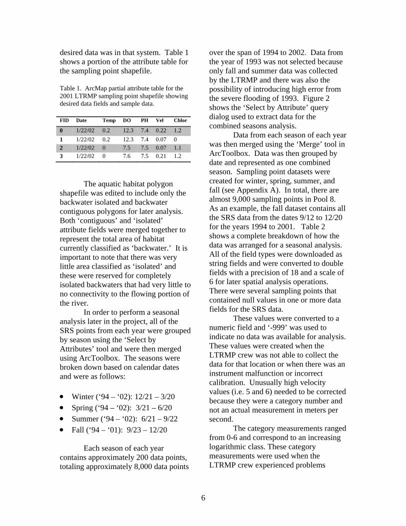
desired data was in that system. Table 1 shows a portion of the attribute table for the sampling point shapefile. Table 1. ArcMap partial attribute table for the 2001 LTRMP sampling point shapefile showing desired data fields and sample data. FID Date Temp DO PH Vel Chlor

0 1/22/02 0.2 12.3 7.4 0.22 1.2 1 1/22/02 0.2 12.3 7.4 0.07 0 2 1/22/02 0 7.5 7.5 0.07 1.1 3 1/22/02 0 7.6 7.5 0.21 1.2

The aquatic habitat polygon shapefile was edited to include only the backwater isolated and backwater contiguous polygons for later analysis. Both ‘contiguous’ and ‘isolated’ attribute fields were merged together to represent the total area of habitat currently classified as ‘backwater.’ It is important to note that there was very little area classified as ‘isolated’ and these were reserved for completely isolated backwaters that had very little to no connectivity to the flowing portion of the river. In order to perform a seasonal analysis later in the project, all of the SRS points from each year were grouped by season using the ‘Select by Attributes’ tool and were then merged using ArcToolbox. The seasons were broken down based on calendar dates and were as follows: • Winter (‘94 – ‘02): 12/21 – 3/20 • Spring (‘94 – ‘02): 3/21 – 6/20 • Summer (‘94 – ‘02): 6/21 – 9/22 • Fall (‘94 – ‘01): 9/23 – 12/20

Each season of each year contains approximately 200 data points, totaling approximately 8,000 data points

over the span of 1994 to 2002. Data from the year of 1993 was not selected because only fall and summer data was collected by the LTRMP and there was also the possibility of introducing high error from the severe flooding of 1993. Figure 2 shows the ‘Select by Attribute’ query dialog used to extract data for the combined seasons analysis.

Data from each season of each year was then merged using the ‘Merge’ tool in ArcToolbox. Data was then grouped by date and represented as one combined season. Sampling point datasets were created for winter, spring, summer, and fall (see Appendix A). In total, there are almost 9,000 sampling points in Pool 8. As an example, the fall dataset contains all the SRS data from the dates 9/12 to 12/20 for the years 1994 to 2001. Table 2 shows a complete breakdown of how the data was arranged for a seasonal analysis. All of the field types were downloaded as string fields and were converted to double fields with a precision of 18 and a scale of 6 for later spatial analysis operations. There were several sampling points that contained null values in one or more data fields for the SRS data.

These values were converted to a numeric field and ‘-999’ was used to indicate no data was available for analysis. These values were created when the LTRMP crew was not able to collect the data for that location or when there was an instrument malfunction or incorrect calibration. Unusually high velocity values (i.e. 5 and 6) needed to be corrected because they were a category number and not an actual measurement in meters per second.

The category measurements ranged from 0-6 and correspond to an increasing logarithmic class. These category measurements were used when the LTRMP crew experienced problems

6

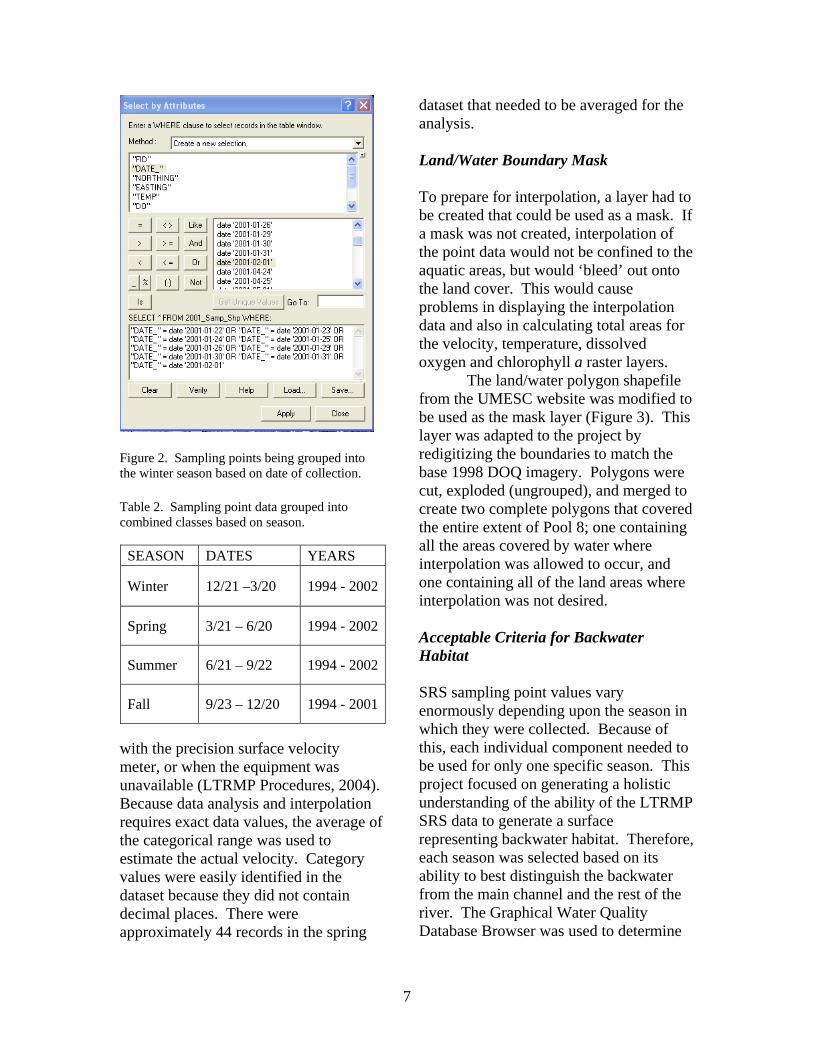
Figure 2. Sampling points being grouped into the winter season based on date of collection. Table 2. Sampling point data grouped into combined classes based on season.

SEASON DATES YEARS

Winter 12/21 –3/20 1994 - 2002

Spring 3/21 – 6/20 1994 - 2002

Summer 6/21 – 9/22 1994 - 2002

Fall 9/23 – 12/20 1994 - 2001

with the precision surface velocity meter, or when the equipment was unavailable (LTRMP Procedures, 2004). Because data analysis and interpolation requires exact data values, the average of the categorical range was used to estimate the actual velocity. Category values were easily identified in the dataset because they did not contain decimal places. There were approximately 44 records in the spring

dataset that needed to be averaged for the analysis. Land/Water Boundary Mask To prepare for interpolation, a layer had to be created that could be used as a mask. If a mask was not created, interpolation of the point data would not be confined to the aquatic areas, but would ‘bleed’ out onto the land cover. This would cause problems in displaying the interpolation data and also in calculating total areas for the velocity, temperature, dissolved oxygen and chlorophyll a raster layers. The land/water polygon shapefile from the UMESC website was modified to be used as the mask layer (Figure 3). This layer was adapted to the project by redigitizing the boundaries to match the base 1998 DOQ imagery. Polygons were cut, exploded (ungrouped), and merged to create two complete polygons that covered the entire extent of Pool 8; one containing all the areas covered by water where interpolation was allowed to occur, and one containing all of the land areas where interpolation was not desired. Acceptable Criteria for Backwater Habitat SRS sampling point values vary enormously depending upon the season in which they were collected. Because of this, each individual component needed to be used for only one specific season. This project focused on generating a holistic understanding of the ability of the LTRMP SRS data to generate a surface representing backwater habitat. Therefore, each season was selected based on its ability to best distinguish the backwater from the main channel and the rest of the river. The Graphical Water Quality Database Browser was used to determine

7

Figure 3. Land / Water boundary polygon shapefile digitized from the 1998 DOQ imagery showing the water polygon as black. the largest degree of separation between backwater and main channel habitat areas. Each component of velocity, temperature, DO, and chlorophyll a was given an acceptable data range that was descriptive of backwater aquatic habitat classification. Since no previous classifications exist, a variety of sources were used to determine the acceptable data ranges. The most important of these sources being the Graphical Water Quality Database Browser found on the UMESC website. To determine data value ranges for each component, an IDW interpolation for each combined season was generated using spatial analyst. Values that fell within areas currently classified as aquatic backwater habitat were selected and averaged to create the acceptable criteria values for

backwater habitat. For example, an IDW interpolation of the velocity sampling points revealed almost all of the data points that were present in the current backwater classification areas had a velocity value of 0.1m/s or less. Using a value slightly greater than 0 m/s allowed backwater contiguous habitat to be included in the new classification criteria. Table 3 shows each LTRMP water chemistry component, the corresponding seasonal data that was chosen, and the acceptable criteria data range that was selected to define backwater aquatic habitat. Inverse Distance Weighted Interpolations Inverse distance weighted (IDW) interpolations were chosen to generate a representative surface of backwater aquatic habitat based on the LTRMP Table 3. LTRMP water chemistry components and their corresponding season chosen for GIS analysis.

LTRMP Component Season Criteria

Velocity ⇒ Spring ≤ 0.1 m/s DO ⇒ Winter ≤ 5ppm

Chlorophyll a ⇒ Summer ≥ 76 mg/L

Temperature ⇒ Spring ≥ 14.5 °C sampling points. The IDW method of interpolation estimates sampling point values by averaging values of neighboring sampling points. IDW gives more weight to estimated values that are closer to the cell being processed. This method of cell estimation works most effectively with a dense pattern of sampling points which is characteristic of the LTRMP data. In addition, IDW interpolation accurately reflects the natural distributions of water chemistry in the pool. Other methods of

8

interpolation such as Kriging were explored, but IDW was the most logical and produced the most predictive results. The spatial analyst extension was used to perform the interpolations. All the values in the attribute table (except those containing the null value, -999) were selected. The land/water boundary layer that was created was used as the mask layer to prevent interpolation onto land areas within the pool. A 5 meter cell size was chosen to simplify area calculations later in the project analysis. A habitat interpolation GRID (termed “HIG”) was created for each LTRMP component and can be viewed in Appendix B. The symbology chosen was consistent to all the HIGs for effective visual comparison and a Jenks natural breaks value grouping was used with 10 classes. It is important to note that these HIGs contain all the measured values for all the sampling points of the specified component in the pool. Analysis Reclassifying Raster Values A binary approach (1,0) was chosen as the analysis method to most effectively address the goals of this project. In order to accomplish this, the HIGs needed to be reclassified into one of two values: ‘1’ or ‘0’. A value of ‘1’ represents that the specified criteria was met, or was true. A value of ‘0’ represents that the specified criteria was not met, or was false. For example, if a cell contained within the velocity HIG had a value of 0.1 m/s, it would be calculated as a ‘1.’ If the value of the cell was 0.2 m/s, it would be calculated as a ‘0.’ The Raster Calculator function of Spatial Analyst was employed to reclass each HIG into the 2 values. No

data values were included in the ‘0’ classification. The reclassified HIGs are shown in Appendix C. Each HIG was now able to reveal the locations of acceptable backwater aquatic habitat criteria for velocity, temperature, chlorophyll a, and dissolved oxygen. Raster Calculator was again used for a combined (suitability) analysis to generate a final output raster that would represent the combined effects of each of the four LTRMP water chemistry components. The following syntax was used to generate the combined raster: CombinedRaster = [Spring_temp] + [Summer_chlor] + [Winter_do] + [Spring_vel] The output raster contained 5 values: 0, 1, 2, 3, and 4. A value of 0 represented that none of the LTRMP component criteria were met, and 4 represented that all of the criteria were met. The output raster was symbolized with both a single color with one class (representing areas where at least one component was met) and also as 4 classes (see Appendix D). This 4 class combined raster is an extremely valuable output of the project. It is able to very accurately determine the locations where the established criteria for backwater aquatic habitat are present and the relative degree to which it is present. LTRMP Combined Raster vs. the Current Backwater Raster Since the goal of this project was to create a surface representing backwater aquatic habitat through interpolation, it is necessary to compare the final combined raster to the current photo interpretation delineated raster available from UMESC and used by several agencies to identify backwater habitats. In order to undergo a

9

comparative analysis between the relative surface areas of the two rasters, the surface area was calculated for each where: Area = cell size * cell count In the case of the current photo interpretation backwater area, it can be calculated that: Area Current = 5 * 5 * 1,057,530 m2 = 26,438,250 m2 = 6,533 acres Using the LTRMP SRS combined data components of temperature, velocity, chlorophyll a, and DO as indicators of backwater aquatic habitat can be calculated by: Area LTRMP = 5 * 5 * 573,433 m2 = 14,335,825 m2 =3,542 acres Given these figures, it can be inferred that the LTRMP combined aquatic backwater raster encompassed approximately 54% of the total area that is classified in the current raster. It is important to note that the LTRMP interpolation method also found several areas in the pool that are not currently classified as backwater habitat. These should be investigated further to determine if they are backwater ‘microhabitats’ or simply abnormalities caused by inconsistencies in the data. An enlarged image of this comparison is shown in Appendix E. Conclusions This project has shown that the LTRMP water chemistry data can be a valuable tool to define backwater aquatic habitat.

Enormous amounts of time and money have been invested in collecting and housing this data and it is reassuring to show that it is extremely valuable. There are large limitations, however, to using the SRS sampling point data to interpolate a surface representing the backwater habitat. As seen in Appendix E, the middle section of the pool (near Goose Island) containing the heavily braided island areas has not been accounted for in the LTRMP combined raster. Although thousands of sampling points were used for the interpolation, this reveals the limitation in using this analysis design. The spatial density of the sampling points is not high enough to account for the enormously detailed nature of the disconnected and maze-like channel islands. In the areas that are considered isolated backwater habitat, almost all of the open area has been accounted for by several of the combined components. This suggests that using the LTRMP criteria should possibly be reserved for identifying isolated backwater habitat or for identifying ‘hot spots’ in the spatially complex water/land interface areas. Nonetheless, this tool will not replace the need for habitat classifications based on geomorphology and photo interpretation. Instead, it will be a valuable tool to locate specific habitat areas defined by the established criteria that is created for each water chemistry component. This project utilized an equal weight analysis and each component was given equal weight in the final analysis. When comparing the water chemistry components individually, it is clear that velocity is able to define backwater aquatic habitat much more intensely than chlorophyll a, for example. Because of this, future data collection procedures in other UMR pools that have more limited budgets could focus data collection on

10

velocity measurements. Chlorophyll a could also be weighted in future analyses or could be amplified by applying a higher power value prior to interpolation. It is important to note that the real strength of this model lies in its ability to be adapted to the needs of the user or river manager. For example, the defining criteria for the water chemistry components can be changed and adapted to define a surface representation of different aquatic habitats on the Upper Mississippi River. Schramm (2004) states the LTRMP should be expanded to include the entire navigable portion of the Mississippi River and the application of geospatial technologies will help monitor system changes and contribute to more effective assessment. This project supports his claims. Using LTRMP water quality data and interpolation methods could also be used for an enormous array of related river projects such as locating critical fish overwintering habitat locations based on their physical water chemistry requirements. Acknowledgements This project would not have been possible without the mentoring and guidance from the following people: John Ebert, for his wholehearted academic encouragement, Patrick Thorsell, for answering every tedious question with enthusiasm, Dr. David McConville, for setting the bar as the genuine scholar, Tom Boland, for his expertise on the Upper Mississippi River and his unwavering support, and lastly to John Sullivan for proposing to me the importance of this project. I would also like to thank my peers and classmates at Saint Mary’s University of Minnesota

for sharing their knowledge and friendship. References

Cobb, S. P. and Clark, J. R. 1980. Aquatic Habitat Studies of the Lower Mississippi, River Miles 480-530. Report 2, Aquatic Habitat Mapping: Miscellaneous Paper E-80-1. U.S. Army Engineers Lower Mississippi Valley Division, Vicksburg, MS.

Nord, R. C. 1967. A Compendium of Fishery Information on the Upper Mississippi River. Upper Mississippi River Conservation Committee. Sec. Publication. 238pp.

Rasmussen, J. and Pitlo, J. 1998. Upper Mississippi River Habitat Classification. Retrieved October 2, 2007 from http://www.mississippi river.com /umrcc/pdf/Fisheries% 20Compendium.pdf

Schramm, H.L. 2004. Status and Management of Mississippi River Fisheries. Retrieved October 15, 2007, from http://www.lars2.org/ Proceedings/vol1/Stats_ Management_of_Mississippi.pdf

Soballe, D. M., and Fischer, J. R. 2004. Long Term Resource Monitoring Program Procedures: Water Quality Monitoring. U.S. Geological Survey, Upper Midwest Environmental Sciences Center, La Crosse, WI, March 2004. Technical Report LTRMP 2004-T002-1 (Ref. 95-P002-5). 73 pp. + Appendixes A – J

Sternberg, R. B. 1971. Upper Mississippi River Habitat Classification Survey. Fish Technical Section Special Report Upper Mississippi River Conservation Committee, 4469-48th. Avenue Court, Rock Island, Illinois.

Theiling, C. 1998. River Geomorphology and Floodplain Habitats. Retrieved October 3, 2007, from http://www.umesc.gov /documents

11

12

/repoxrts/1999/staus_and_trends/ 99t001_ ch041r.pdf

Wilcox, D. B. 1993. An Aquatic Habitat Classification System for the Upper Mississippi River System. U.S. Fish and Wildlife Service, Environmental Management Technical Center, Onalaska, WI. EMTC 93-T003. 9pp. + Appendix A. USGS July, 2003.

USGS July, 2003. Nutrients in the Upper Mississippi River: Scientific Information to Support Management Decisions. Retrieved October 1, 2007, from http://pubs.usgs.gov/fs/2003/fs- 105-03/pdf/nutrient_umrs.pdf

USGS June, 2006. Taking the Pulse of a River System: First 20 Years. Retrieved October 1, 2007, from http://pubs.usgs.gov/fs/2006 /3098/pdf/FS2006-3098.pdf

Appendix A. LTRMP Stratified Random Sampling Points in Pool 8 of the UMR.

Winter – 1,544 sampling points (gray) Spring – 1,536 sampling points (green)

13

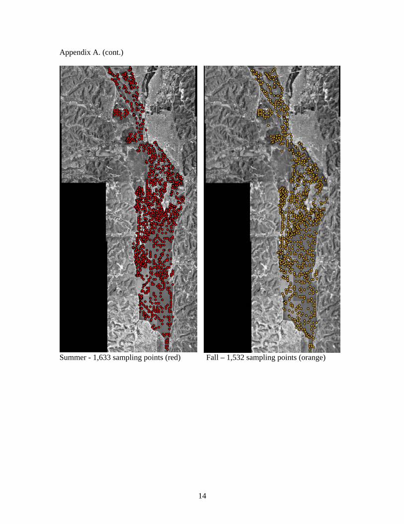
Appendix A. (cont.)

Summer - 1,633 sampling points (red) Fall – 1,532 sampling points (orange)

14

Appendix B. IDW Interpolations of SRS LTRMP Water Chemistry Data.

Winter DO (ppm) Spring Velocity (meters/second)

15

Appendix B. (cont.)

Summer Chlorophyll (micrograms/L) Spring Temperature (˚C)

16

Appendix C. Reclassified Raster Data.

Winter DO ≤ 5ppm (green) Spring Velocity ≤ 0.1 m/s (red)

17

Appendix C. (cont.)

Summer Chlorophyll a ≥ 76 mg/L (blue) Spring Temperature ≥ 14.5 °C (purple)

18

Appendix D. Combined Analysis Raster Data.

Combined Raster Data (One Color) One or more criteria met = blue One c teria m

Combined Raster Data (Four Color) ri et = light purple

Four criteria met = dark purple

19

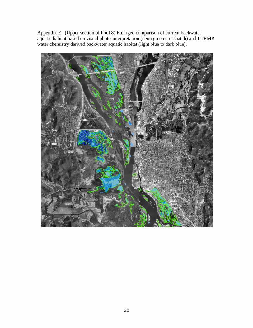
Appendix E. (Upper section of Pool 8) Enlarged comparison of current backwater aquatic habitat based on visual photo-interpretation (neon green crosshatch) and LTRMP water chemistry derived backwater aquatic habitat (light blue to dark blue).

20

Appendix E. (Middle section of Pool 8)

21

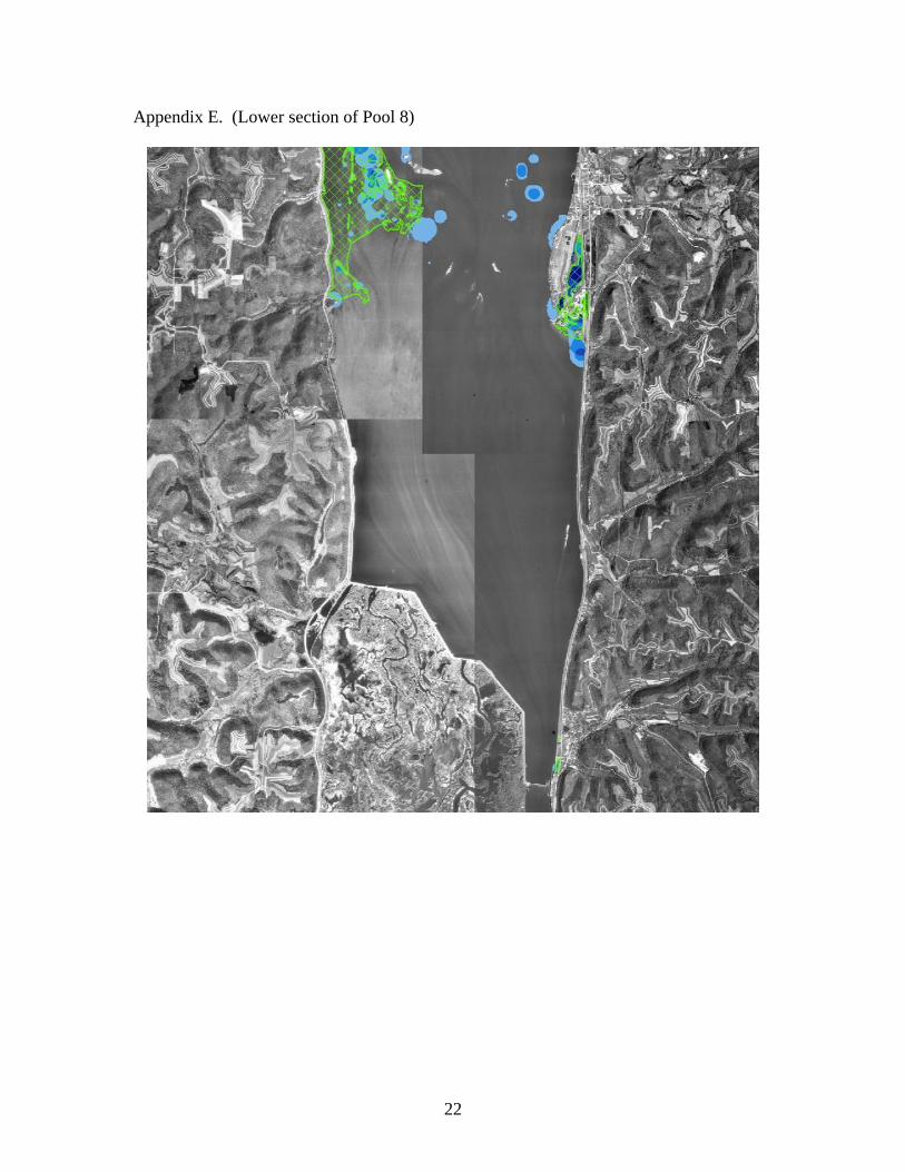
A

22

ppendix E. (Lower section of Pool 8)