arX

iv:a

stro

-ph/

0506

030v

1 2

Jun

200

5

Systematic Errors in Future Weak Lensing Surveys: Requirements and

Prospects for Self-Calibration

Dragan HutererKavli Institute for Cosmological Physics and Astronomy and

Astrophysics Department, University of Chicago, Chicago, IL 60637

Masahiro TakadaAstronomical Institute, Tohoku University, Sendai 980-8578, Japan

Gary Bernstein and Bhuvnesh JainDepartment of Physics and Astronomy, University of Pennsylvania, Philadelphia, PA 19104

We study the impact of systematic errors on planned weak lensing surveys and compute therequirements on their contributions so that they are not a dominant source of the cosmological pa-rameter error budget. The generic types of error we consider are multiplicative and additive errors inmeasurements of shear, as well as photometric redshift errors. In general, more powerful surveys havestronger systematic requirements. For example, for a SNAP-type survey the multiplicative error inshear needs to be smaller than 1% (fsky/0.025)

−1/2 of the mean shear in any given redshift bin, while

the centroids of photometric redshift bins need to be known to better than 0.003 (fsky/0.025)−1/2 .

With about a factor of two degradation in cosmological parameter errors, future surveys can entera self-calibration regime, where the mean systematic biases are self-consistently determined fromthe survey and only higher-order moments of the systematics contribute. Interestingly, once thepower spectrum measurements are combined with the bispectrum, the self-calibration regime in thevariation of the equation of state of dark energy wa is attained with only a 20-30% error degradation.

I. INTRODUCTION

There has been significant recent progress in the measurements of weak gravitational lensing by large scale structure.Only five years after the first detections made by several groups (Wittman et al. 2000, Bacon et al. 2000, van Waerbekeet al. 2000, Kaiser et al. 2000), weak lensing already imposes strong constraints on the matter density relative to criticalΩM and the amplitude of mass fluctuations σ8 (Hoekstra, Yee & Gladders 2002, Jarvis et al. 2003, Rhodes et al. 2004,Heymans et al. 2004; for a review see Refregier 2003), as well as the first interesting constraints on the equation ofstate of dark energy (Jarvis et al. 2005).The main advantage of weak lensing is that it directly probes the distribution of matter in the universe. This makes

weak lensing a powerful probe of cosmological parameters, including those describing dark energy (Hu & Tegmark1999, Huterer 2002, Hu 2003a, Heavens 2003, Refregier et al. 2003, Benabed & Van Waerbeke 2004, Takada & Jain2004, Takada & White 2004, Song & Knox 2004, Ishak et al. 2004, Ishak 2005). The weak lensing constraints areespecially effective when some redshift information is available for the source galaxies; use of redshift tomography canimprove the cosmological constraints by factors of a few (Hu 1999). Furthermore, measurements of the weak lensingbispectrum (Takada & Jain 2004) and purely geometrical tests (Jain & Taylor 2003, Bernstein & Jain 2004, Zhanget al. 2003, Song & Knox 2004, Hu & Jain 2004, Bernstein 2005) lead to significant improvements of accuracy inmeasuring the cosmological parameters. When these methods are combined, weak lensing by itself is expected toconstrain the equation of state of dark energy w to a few percent, and impose interesting constraints on the timevariation of w. Ongoing or planned surveys, such as the Canada-France-Hawaii Telescope Legacy Survey1, the DarkEnergy Survey2 (DES), PanSTARRS3 and VISTA4 are expected to significantly extend lensing measurements, whilethe ultimate precision will be achieved with the SuperNova/Acceleration Probe5 (SNAP; Aldering et al. 2004) andthe Large Synoptic Survey Telescope6 (LSST).However, so far the rosy weak lensing parameter accuracy predictions that have appeared in literature have not

1 http://www.cfht.hawaii.edu/Science/CFHLS2 http://cosmology.astro.uiuc.edu/DES3 http://pan-starrs.ifa.hawaii.edu4 http://www.vista.ac.uk5 http://snap.lbl.gov6 http://www.lsst.org

2

allowed for the presence of systematics (exceptions are Ishak et al. (2004) and Knox et al. (2005) who consider a shearcalibration error, and Bernstein (2005) who does the same for the cross-correlation cosmography of weak lensing).This is not surprising, as we are just starting to understand and study the full budget of systematic errors present inweak lensing measurements. Nevertheless, some recent work has addressed various aspects of the systematics, bothexperimental and theoretical, and ways to correct for them. For example, Vale et al. (2004) estimated the effects ofextinction on the extracted shear power spectrum, while Hirata & Seljak (2003), Hoekstra (2004) and Jarvis & Jain(2004) considered the errors in measurements of shear. Several studies explored the effect of theoretical uncertainties(White 2004, Zhan & Knox 2004, Huterer & Takada 2004) and ways to protect against their effects (Huterer & White2005). It has been pointed out that second-order corrections in the shear predictions can be important (Schneider etal. 2002, Hamana et al. 2002, Cooray & Hu 2002, White 2005, Dodelson & Zhang 2005, Dodelson et al. 2005).Despite these efforts, we are at an early stage in our understanding of weak lensing systematics. Realistic assessments

of systematic errors is likely to impact strategies for measuring the weak lensing shear (Bernstein 2002, Bernstein &Jarvis 2002, Rhodes et al. 2004, Mandelbaum et al. 2005). Eventually we would like to bring weak lensing to thesame level as cosmic microwave background anisotropies (CMB) and type Ia supernovae, where the systematic errorbudget is better understood and requirements for the control of systematic precisely outlined (e.g. Tegmark et al.2000, Hu, Hedman & Zaldarriaga 2003, Kim et al. 2003, Linder & Miquel 2004).The purpose of this paper is to introduce the framework for the discussion of systematic errors in weak lensing

measurements and outline requirements for several generic types of systematic error. The reason that we do not

consider specific sources of error (e.g. temporal variations in the telescope optics or fluctuations in atmospheric seeing)is that there are many of them, they strongly depend on a particular survey considered, and they are often poorlyknown before the survey has started collecting data. Instead we argue that, at this early stage of our understandingof weak lensing systematics, it is more practical and useful to consider three generic types of error – multiplicativeand additive error in measurements of shear, as well as redshift error. These generic errors are useful intermediatequantities that link actual experimental sources of error to their impact on cosmological parameter accuracy. Infact, realistic systematic errors for any particular experiment can in general be converted to these three genericsystematics. Given the specifications of a particular survey, one can then estimate how much a given systematicdegrades cosmological parameters. This can be used to optimize the design of the experiment to minimize the effectsof systematic errors on the accuracy of desired parameter. For example, accurate photometric redshift requirementswill lead to requirements on the number of filters and their wavelength coverage. Similarly, the requirements onmultiplicative and additive errors in shear will determine how accurate the sampling of the point spread functionneeds to be.The plan of the paper is as follows. In § II we discuss the survey specifications and cosmological parameters in this

study. In § III we describe the parameterization of systematic errors. In § IV-VI we present the requirements on thesystematic errors for the power spectrum, while in § VII we study the requirements when both the power spectrumand the bispectrum are used. We combine the redshift and multiplicative errors and discuss trends in § VIII andconclude in § IX.

II. METHODOLOGY, COSMOLOGICAL PARAMETERS AND FIDUCIAL SURVEYS

We express the measured convergence power spectrum as

Cκij(ℓ) = P κ

ij(ℓ) + δijσ2γ

ni, (1)

where P κij(ℓ) is the measured power spectrum with systematics (see the next Section on how it is related to the

no-systematic power spectrum P κij(ℓ)), σ

2γ is the variance of each component of the galaxy shear and ni is the average

number of resolved galaxies in the ith redshift bin per steradian. The convergence power spectrum at a fixed multipoleℓ and for the ith and jth redshift bin is given by

P κij(ℓ) =

∫

∞

0

dzWi(z)Wj(z)

r(z)2 H(z)P

(

ℓ

r(z), z

)

, (2)

where r(z) is the comoving angular diameter distance and H(z) is the Hubble parameter. The weights Wi are givenby

Wi(χ) =3

2ΩM H2

0 gi(χ) (1 + z) (3)

3

DES SNAP LSST

Area (sq. deg.) 5000 1000 15000

n (gal/arcmin2) 10 100 30

σγ 0.16 0.22 0.22

zpeak 0.5 1.0 0.7

TABLE I: Fiducial sky coverage, density of source galaxies, variance of (each component of) shear of one galaxy, and peak ofthe source galaxy redshift distribution for the three surveys considered.

where gi(χ) = r(χ)∫

∞

χdχsni(χs)r(χs − χ)/r(χs), χ is the comoving radial distance and ni is the fraction of galaxies

assigned to ith redshift bin. We employ the redshift distribution of galaxies of the form

n(z) ∝ z2 exp(−z/z0) (4)

where z0 is survey dependent and specified below. The cosmological constraints can then be computed from the Fishermatrix

Fij =∑

ℓ

(

∂C

∂pi

)T

Cov−1 ∂C

∂pj, (5)

where C is the column matrix of the observed power spectra and Cov−1 is the inverse of the covariance matrix

between the power spectra whose elements are given by

Cov[

Cκij(ℓ

′), Cκkl(ℓ)

]

=δℓℓ′

(2ℓ+ 1) fsky ∆ℓ

[

Cκik(ℓ)C

κjl(ℓ) + Cκ

il(ℓ)Cκjk(ℓ)

]

. (6)

Here ∆ℓ is the band width in multipole we use, and fsky is the fractional sky coverage of the survey.In addition to any nuisance parameters describing the systematics, we consider six or seven cosmological parameters

and assume a flat universe throughout. The six standard parameters are energy density and equation of state of darkenergy ΩDE and w, spectral index n, matter and baryon physical densities ΩMh2 and ΩBh

2, and the amplitude of massfluctuations σ8. Note that w = const provides useful information about the sensitivity of an arbitrary w(z), since thebest-measured mode of any w(z) is about as well measured as w = const and therefore is subject to similar degradationsin the presence of the systematics. It is this particular mode, being the most sensitive to generic systematics, that willdrive the accuracy requirements – we explicitly illustrate this in Fig. 2. In addition to the constant w case, we alsoconsider a commonly used two-parameter description of dark energy w(z) = w0 + waz/(1 + z) (Linder 2003) wherewa becomes the seventh cosmological parameter in the analysis. Throughout we consider lensing tomography with7-10 equally spaced redshift bins (see below), and we use the lensing power spectra on scales 50 ≤ ℓ ≤ 3000. We holdthe total neutrino mass fixed at 0.1 eV; the results are somewhat dependent on the fiducial mass. We compute thelinear power spectrum using the fitting formulae of Eisenstein & Hu (1999). We generalize the formulae to w 6= −1by appropriately modifying the growth function of density perturbations. To complete the calculation of the fullnonlinear power spectrum we use the fitting formulae of Smith et al. (2003).The fiducial surveys, with parameters listed in Table II, are: the Dark Energy Survey; SNAP; and LSST. Note that

there is some ambiguity in the definition of the number density of galaxies ng; it is the quantity σ2γ/ng that determines

the shear measurement noise level, where σγ is the intrinsic shape noise of each galaxy. The surveys are assumed tohave the source galaxy distribution of the form in Eq. (4) which peaks at zpeak = 2z0. For the fiducial SNAP andLSST surveys we assume tomography with 10 redshift bins equally spaced out to z = 3, as future photometric redshiftaccuracy will enable relatively fine slicing in redshift. For the DES, we assume a more modest 7 redshift bins out toz = 2.1, reflecting the shallower reach of the DES while keeping the redshift bins equally wide (∆z = 0.3) as in theother two surveys. Finally, we do not use weak lensing information beyond ℓ = 3000 in order to avoid the effects ofbaryonic cooling (White 2004, Zhan & Knox 2004, Huterer & Takada 2004) and non-Gaussianity (White & Hu 2000,Cooray & Hu 2001), both of which contribute more significantly at smaller scales. While there may be ways to extendthe useful ℓ-range to smaller scales without risking bias in cosmological constraints (Huterer & White 2005), extendingthe measurements to ℓmax = 10000 would improve the marginalized errors on cosmological parameters by only about

4

30%7. The parameter fiducial values and accuracies are summarized in Table II near the end of the article. Thefiducial values for the parameters not listed in Table II are ΩMh2 = 0.147, ΩBh

2 = 0.021, n = 1.0, and mν = 0.1eV.It is well known that measurements of the angular power spectrum of the CMB, such as those expected by the

Planck experiment, can help weak lensing constrain the cosmological parameters. In particular, the morphology of thepeaks in the CMB angular power spectrum contains useful information on the physical matter and baryon densities,while the locations of the peaks help constrain the dark energy parameters. However we checked that, when the Planckprior added, all systematics requirements become weaker (relative to those with weak lensing alone) since the Planckinformation is not degraded with systematic errors even if weak lensing information is. In order to be conservative,we decided not to add the Planck CMB information. Therefore, we consider the systematics requirements in weaklensing surveys alone, and note that addition of complementary information from other surveys typically weakensthese requirements.

III. PARAMETERIZATION OF THE SYSTEMATICS

As mentioned above, we consider three generic sources of error. We believe that the parameterizations we propose,especially for the redshift and multiplicative shear errors, are general enough to account for the salient effects of anygeneric systematic. The additive shear error is more model-dependent, and while we motivate a parameterization webelieve is reasonable at this time, further theoretical and experimental work needs to be done to understand additiveerrors.We parameterize the redshift, multiplicative shear and additive shear errors as follows.

A. Redshift Errors

Measurements of galaxy redshifts are necessary not only for the redshift tomography – which significantly improvesthe accuracy in measuring dark energy parameters – but also to obtain the fiducial distribution of galaxies in redshift,n(z). Therefore, understanding and correcting for the redshift uncertainties is crucial, and comparison studies betweencurrently used photometric methods, such as that initiated by Cunha et al. (2005), are crucial.It is important to emphasize that statistical errors in photometric redshifts do not contribute to the error budget

if they are well characterized. In other words, if we know precisely the distribution of photometric redshift errors(that is, all of its moments) at each redshift, we can use the measured photometric distribution, np(zp), to recover theoriginal spectroscopic distribution, n(zs) very precisely. In practice we will not know the redshift error distributionwith arbitrary precision, rather we will typically have some prior knowledge of the mean bias and scatter at eachredshift.The quantity we consider in this paper is the uncalibrated redshift bias, that is, the residual (after correcting for

the estimated bias) offset between the true mean redshift and the inferred mean photometric redshift at any givenz. A more general description of the redshift error would include the scatter in the redshift error at each z. Suchan analysis has recently been performed by Ma, Hu & Huterer (2005) who found that, even though the scatter isimportant as well, the mean bias in redshift is the dominant source of error.Unlike Ma, Hu & Huterer (2005) who hold the overall distribution of galaxies in redshift n(z) fixed and only allow

variations in the tomographic bin subdivisions, we allow the redshift error to affect the overall n(z) as well. At thistime it is not clear how the photometric error will affect the source galaxy distribution n(z) as it depends on how thesource galaxy distribution will be determined. We assume that the source galaxy distribution n(z) is obtained fromthe same photometric redshifts used to subdivide the galaxies into redshift bins. An alternative possibility is thatinformation about the overall distribution of source galaxies is obtained from an independent source (say, anothersurvey) while the internal photometric redshifts are only used to subdivide the overall distribution into redshift bins.The two approaches, ours and that of Ma, Hu & Huterer (2005), are therefore complementary and both should bestudied. As discussed in the conclusions, it is reassuring that the two approaches give consistent results.We consider two alternative parameterizations of the redshift error: the centroids of redshift bins, and the Chebyshev

polynomial expansion of the mean bias in the zp − zs relation. We now describe them.

Centroids of redshift bins. We first consider the centroid of each photometric redshift bin as a parameter. Any

7 On the other hand, especially for the DES, the Gaussian covariance assumption may be somewhat optimistic for the range 1000 < ℓ <

3000 (e.g. White & Hu 2000).

5

scatter in galaxy redshifts in a given tomographic bin will average out, to first order leaving the effect of an overallbias in the centroid of this bin. [Recall, the part of the bias that is uncalibrated and has not been subtracted out iswhat we consider here.] As discussed by Huterer et al. (2004) in the context of number-count surveys, this approachcaptures the salient effects of the redshift distribution uncertainty. Note, however, that the centroid shifts do notcapture the “catastrophic” errors where a smaller fraction of redshifts are completely misestimated and reside in aseparate island in the zp − zs plane.We therefore have B new parameters, where B is the number of redshift bins. To compute the Fisher derivatives

for these parameters, we vary each centroid by some value dz, that is, we shift the whole bin by dz. As mentionedabove, this procedure not only allows for the fact that the tomographic bin divisions are not perfectly measured, butit also deforms the overall distribution of galaxies n(z).

Expansion of the redshift bias in Chebyshev polynomials. While the required accuracy of redshift bin centroidsprovides useful information, it is sometimes difficult to compare it with directly observable quantities. In reality, anobserver typically starts with measurements of photometric redshifts which are not equal to the true, spectroscopicones: the quantity zp − zs may have a nonzero value — the bias – and also nonzero scatter around the biased value.Therefore, it is sometimes more useful to consider requirements on the accuracy in the zp − zs relation.Detailed forms of the bias and scatter are typically complicated and depend on the photometric method used and

how well we are able to mimic the actual observations and correct for the biases. We write the redshift bias as a sumof Ncheb smooth functions – Chebyshev polynomials centered at zmax/2 and extending from z = 0 to z = zmax, wherezmax (3.0 for SNAP and LSST, 2.1 for the DES) is the extent of the distribution of galaxies in redshift. [We brieflyreview the Chebyshev polynomials in the Appendix.] The relation between the photometric and true, spectroscopicredshifts is then

zp = zs +

Ncheb∑

i=1

giTi(z∗

s ), where (7)

z∗s ≡zs − zmax/2

zmax/2, (8)

and gi are the coefficients that parameterize the bias. As with the centroids of redshift bins, we do not model thescatter in the zp−zs relation as one can show that the effect of uncalibrated bias is dominant (Ma, Hu & Huterer, 2005).The effect of imperfect redshift measurements is to shift the distribution of galaxies away from the true distributionn(zs) to a biased one np(zp). The biased distribution of galaxies then propagates to bias the cosmological parameters.The photometric distribution can then simply be obtained from the true distribution as (e.g. Padmanabhan et al.2005)

np(zp) =

∫

∞

0

n(z)∆(zp − z, z)dz (9)

where ∆(zp − z, z) is the probability that the galaxy at redshift z is measured to be at redshift zp. Since we are notmodeling the scatter in the zp − zs relation, the probability is a delta function

∆(zp − z, z) = δ

(

zp − zs −

Ncheb∑

i=1

giTi(z∗

s )

)

. (10)

Since we will include the gi as additional parameters, with fiducial values gi = 0, we shall need to take derivativeswith one nonzero gi at a time and therefore we can assume ∆(zp − z, zp) = δ(zp − zs − giTi(z

∗

s )) for a single i. Usingthe fact that δ(F (x)) =

∑

1/|F ′(x0)| δ(x−x0) for a function F (z), where the sum runs over the roots of the equationF (x) = 0, and further using a recursive formula for the derivative of the Chebyshev polynomial (Arfken 2000, § 13.3),we get

np(zp) =∑

a

n(za)∣

∣

∣

∣

1 + 2gizmax[1− (z∗a)

2][−izaTi(z

∗

a) + iTi−1(z∗

a)]

∣

∣

∣

∣

(11)

6

0 0.5 1 1.5 2 2.5 3z

p

0

0.5

1

n p(zp)

1

2

7

DES

0 0.5 1 1.5 2 2.5 3z

p

0

0.5

1

n p(zp)

1

27

SNAP

FIG. 1: Select three modes (first, second and seventh) of perturbation to the distribution of galaxies n(z) for the DES (left)and SNAP (right), shown together with the original unperturbed distribution (dashed curve in each panel). These three modescorrespond to the modes of perturbation in the zp−zs relation shown in Fig. 9 in the Appendix. Note that SNAP’s fiducial n(z)is broader, making the resulting wiggles in np(zp) less pronounced and the weak lensing measurements therefore less susceptibleto the redshift biases. Note also that the allowed perturbations to n(z) are not only located near the peak of the distribution,but can also have significant wiggles near the tails of the distribution.

where the sum runs over all roots of the equation z+giTi(z∗)−zp = 0, with (recall) z∗a ≡ (za−zmax/2)/(zmax/2). This

is the expression for the perturbed distribution of galaxies due to a single perturbation mode.8 We use it, togetherwith the original distribution n(z), to compute the perturbed and unperturbed convergence power spectra and thustake the derivative with respect to gi.In Fig. 1 we show the photometric galaxy distributions np(zp) for the select three Chebyshev modes (first, second

and seventh) of perturbation to the distribution of galaxies n(z) corresponding to Fig. 9, together with the originalunperturbed distribution. The distributions are shown for the DES and SNAP. Since the incorrect assignment ofphotometric redshifts only redistributes the galaxies, we always impose the requirement

∫

∞

0 np(zp)dzp = 1 regardlessof the perturbation. Note that SNAP’s fiducial n(z) is broader, making the resulting wiggles in np(zp) less pronouncedand helping the weak lensing measurements be less susceptible to the redshift biases. (As shown in § IVA, this effectis counteracted by the smaller fiducial errors in the SNAP survey which lead to more susceptibility to biases.)

B. Multiplicative errors

The multiplicative error in measuring shear can be generated by a variety of sources. For example, a circular PSFof finite size is convolved with the true image of the galaxy to produce the observed image, and in the process itintroduces a multiplicative error. Let γ(zs,n) and γ(zs,n) be the estimated and true shear of a galaxy at some true(spectroscopic) redshift zs and direction n. Then the general multiplicative factor fi(θ) acts as

γ(zs,n) = γ (zs,n)× [1 + fi(zs,n)] (12)

where fi is the multiplicative error in shear which is both direction and time dependent. We can write the error as asum of its mean (average over all directions and redshifts in that tomographic bin) and a component with zero mean,

f(zs,i,n) = fi + ri(n) (13)

8 Note that, for gi ≪ 1, Eq. (11) simplifies to np(zp) = n(zp − giTi(z∗

p))

7

where 〈f(zs,i,n)〉 = fi and 〈ri(n)〉 = 0 and the averages are taken over angle and over redshift within the ith redshiftbin. Then we can write

〈γ(zs,i,n) γ(zs,j ,n+ dn)〉 = 〈γ(zs,i,n) γ(zs,j ,n+ dn) (1 + f(zs,i,n)) (1 + f(zs,j,n))〉 (14)

≃ 〈γ(zs,i,n)γ(zs,j ,n+ dn)〉(1 + fi + fj) (15)

where we dropped terms of order 〈γ γ fifj〉. Since the random component of the multiplicative error is uncorrelatedwith shear, all terms of the form 〈γ γ r〉 are zero. Finally, terms of the form 〈γ γ r r〉 are taken to be small, thusrequiring that 〈ri(n) rj(n+ dn)〉 is smaller than fi and fj (Guzik and Bernstein, 2005). Therefore

P κij(ℓ) = P κ

ij(ℓ)× [1 + fi + fj] (16)

where again we emphasize that fi is the irreducible part of the multiplicative error in ith redshift bin (i.e. its averageover all directions and the ith redshift slab). It is clear that multiplicative errors are potentially dangerous, since theylead to an error that goes as fi and not f2

i . Finally, note that shear calibration is likely to depend on the size of thegalaxy, so that the mean error fi is the error averaged over all galaxy sizes in bin i.

C. Additive errors

Additive error in shear is generated, for example, by the anisotropy of the PSF. We define the additive error via

γ(zs,n) = γ(zs,n) + γadd(zs,n) (17)

Let us assume that the additive error is uncorrelated with the true shears so that the term 〈γ(n)γadd(n)〉 is zero.Furthermore, let the Legendre transform of the term 〈γadd(n)γadd(n)〉 be P κ

add(ℓ). Then we can write

P κij(ℓ) = P κ

ij(ℓ) + P κadd(ℓ). (18)

We now have to specify the additive systematic power P κadd(ℓ). Consider some known sources of additive error: for

example, the additive error induced due to a non-circular PSF is roughly RePSF where ePSF is the ellipticity of thePSF and R ≡ (sPSF/sgal)

2 is the ratio of squares of the PSF and galaxy size (E. Sheldon, private communication);galaxies that are smaller therefore have a larger additive error. Of course, the observer needs to correct the overalltrend in the error, leaving only a smaller residual, and the impact of this residual is what we are interested in. Itshould be clear from this discussion that the additive error in shear can be calibrated by a part that depends on theaverage size of a galaxy at a given redshift multiplied by a random component that depends on the part of the skyobserved. Therefore, we write the additive shear as γadd(zs,i,n) = bir(n) where bi is the characteristic additive shearamplitude in the ith redshift bin and r(n) is a random fluctuation.In multipole space, the two point function can then be expressed as bibj times the angular part which only depends

on |ni −nj |. Note that the additive error for two galaxies at different redshifts (i.e. when i 6= j) is not zero, althoughit may in principle be suppressed relative to the additive error for the auto-power spectra (when i = j). Motivatedby such considerations, we assume the additive systematic in multipole space of the form

P κadd,ij(ℓ) = ρ bibj

(

ℓ

ℓ∗

)α

(19)

where the correlation coefficient ρ describes correlations between bins. The coefficient ρ is always set to unity fori = j, and for i 6= j it is fixed to some fiducial value (not taken as a parameter in the Fisher matrix). While thediscussion above would imply that ρ = 1 for all i and j, we allow for the possibility that the additive errors are notperfectly correlated across redshift bins. In the extreme case of uncorrelated additive errors in different z bins, thecross-power spectra are not affected, ρ = δij . We shall see that the results are weakly dependent on the fiducial valueof ρ unless if ρ = 1 identically.For the multipole dependence of P κ

add we assume a power-law form, and marginalize over the index α. We chooseℓ∗ = 1000, near the “sweet spot” of weak lensing surveys, but note that this choice is arbitrary and made solely forour convenience since ℓ∗ is degenerate with the parameters bi. Our a priori expectation for the value of α is uncertain,and we try several possibilities but find (as discussed later) that the results are insensitive to the value of α. Wetherefore have a total of B + 1 nuisance parameters for the additive error (B parameters bi, plus α).

8

In practice there is no particular reason why an additive systematic would be expected to conform to a power law,so in the future we should consider an additive systematic with more freedom in its spatial behavior. The currenttreatment is optimistic: fixing the systematic to a power law gives it an identifying characteristic that allows us todistinguish it from cosmological signals. Without such a characteristic, the systematic could be much more damaging.

D. Putting the systematics together

With the systematic errors we consider, the resulting theoretical convergence power spectrum is

P κij(ℓ) ≡ P κ(ℓ, z(i)s , z(j)s ) = P κ

(

ℓ, z(i)s + δz(i)p , z(j)s + δz(j)p

)

× [1 + fi + fj] + ρ bibj

(

ℓ

ℓ∗

)α

. (20)

The derivatives with respect to the multiplicative and additive parameters are trivial since they enter as linear

(or power-law) coefficients, while the derivatives with respect to the redshift parameters δz(k)p (really, parameters gi

defined in Eq. (7)) need to be taken numerically.

IV. RESULTS: REDSHIFT SYSTEMATICS

A. Centroids of redshift bins

We have a total of N+B parameters, and we marginalize over the B redshift bin centroids by giving them identicalGaussian priors. While the actual redshift accuracy may be better in some redshift ranges than in others, the requiredaccuracy that we obtain in our approach will pertain to the redshift bins where observations are most sensitive (i.e.at intermediate redshifts z ∼ 0.5− 1).Figure 2 shows the degradation in ΩM , σ8 and w = const, and also w0 and wa, accuracies as a function of our

prior knowledge of the redshift bin centroids. Here and in the subsequent two Figures, the plots are shown separatelyfor each of the three surveys (DES, SNAP and LSST). Since we are using the Fisher matrix formalism withoutexternal priors on cosmological parameters, the cosmological parameter degradations (as well as accuracies) clearly

remain unchanged for an arbitrary fsky if we also scale the priors on the nuisance parameters by f−1/2sky . In these

and subsequent plots we show the degradations for fiducial values of the sky coverage for each survey fsky,fid, wherefsky,fid = f5000, f1000 and f15000 for DES, SNAP and LSST respectively, while indicating that the requirements scale

as (fsky/fsky,fid)−1/2.

We generally find that the degradations in different cosmological parameters are comparable. To have less than∼ 50% degradation, for example, we need to control the redshift centroid bias to about 0.003 (fsky/fsky,fid)

−1/2 for the

DES and SNAP and to about 0.0015 (fsky/fsky,fid)−1/2 for the LSST. The current statistical accuracy in individual

galaxy redshifts is of order 0.02-0.05. Averaging the large number of galaxies in a given redshift bin, it may be thatwe are already close to the aforementioned requirement on the centroid bias, but this will of course depend on thecontrol of systematics in the photometric procedure.As mentioned in the Introduction, the accurately determined combination of w0 and wa, F (w0, wa), is degraded in

nearly the same way as constant w; this is illustrated by a thick dashed line in each panel of Fig. 2. In the rest of thepaper we do not repeat plotting the curves corresponding to F (w0, wa) which nearly overlap those corresponding tow = const. Finally, we show the degradations for w0 and wa separately. Since these two parameters are determinedto a substantially lower accuracy than w = const (see Table II), it is not surprising that the degradations in thesetwo are substantially smaller.

B. Chebyshev expansion in zp − zs

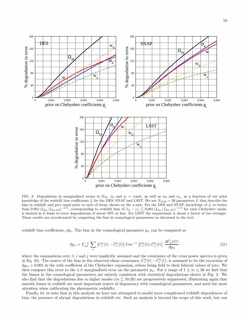
Figure 3 shows the degradation in the ΩM , σ8 and w, and also w0 and wa, as we marginalize over a large number(Ncheb = 30) of Chebyshev coefficients fi each with the given prior. We checked that, when only N <

∼ 5 modes areallowed to vary, all parameters fi can be self-consistently solved from the survey – this is an example of self-calibration.However, with a larger number of Chebyshev modes the self-calibration regime is lost. Since we are interested in themost general form of the redshift bias, this is the regime we would like to explore. We have also checked that, as welet the number of coefficients increase further, the errors in cosmological parameters do not increase indefinitely, asthe rapid fluctuations in the zp − zs are not degenerate with cosmology. In fact we found that the degradations have

9

0 0.002 0.004 0.006 0.008 0.01

prior on centroids of redshift bins

0

20

40

60

80

100

120

140

160

180

200

% d

egra

dati

on in

err

or

ΩM

σ8

w or F(w0, w

a)

DES

w0

wa

0 0.002 0.004 0.006 0.008 0.01

prior on centroids of redshift bins

0

20

40

60

80

100

120

140

160

180

200

% d

egra

dati

on in

err

or ΩM σ

8

w or F(w0, w

a)

SNAP

w0

wa

0 0.002 0.004 0.006 0.008 0.01

prior on centroids of redshift bins

0

20

40

60

80

100

120

140

160

180

200

% d

egra

dati

on in

err

or

ΩM

σ8

w or F(w0, w

a)LSST

w0

wa

FIG. 2: Degradation in the cosmological parameter accuracies as a function of our prior knowledge of δz ≡ zp − zs. We assumeequal Gaussian priors to each redshift bin centroid, shown on the x-axis. For example, to have less than ∼ 50% degradation inΩM , σ8 or w, we need to control the redshift bias to about 0.003 (fsky/fsky,fid)

−1/2 or better for the DES and SNAP, and to

about 0.0015 (fsky/fsky,fid)−1/2 or better for the LSST. For the varying equation of state parameterization, the requirements

for the best measured combination of w0 and wa (F (w0, wa)) are identical to those for w = const, while the requirements onw0 and wa individually are somewhat less stringent.

asymptoted to their final values once we include 20-30 Chebyshev polynomials; therefore, fluctuations in redshift onscales smaller than ∆z ∼ 0.1 are not degenerate with cosmological parameters. The choice of Ncheb = 30 coefficientsis therefore conservative.Figure 3 shows that the photometric redshift bias in each Chebyshev mode, for the DES and SNAP, should be

controlled to about 0.001 (fsky/fsky,fid)−1/2 or less. For LSST, the requirement is more severe and we could tolerate

biases no larger than about 0.0005 (fsky/fsky,fid)−1/2. These are fairly stringent requirements, in rough agreement

with results found by Ma, Hu & Huterer (2005).It might seem a bit surprising that the SNAP and DES requirements are comparable, given that the fiducial SNAP

survey is more powerful than the DES (see Table II) and hence would need better control of the systematics. However,there is another effect at play here: a narrow distribution of galaxies in redshift, such as that from the DES, is morestrongly subjected to fluctuations in zp − zs than a wide distribution, such as that from SNAP; see Fig. 1. Therefore,surveys with wide leverage in redshift have an advantage in beating down the effect of redshift error, just as in thecase of cluster count surveys (Huterer et al. 2004).

We now confirm the results by computing the bias in the cosmological parameters due to the bias in one of the

10

0 0.001 0.002 0.003 0.004 0.005

prior on Chebyshev coefficients gi

0

40

80

120

160

200

% d

egra

dati

on in

err

or

ΩM σ

8

w

DES

wa

w0

0 0.001 0.002 0.003 0.004 0.005

prior on Chebyshev coefficients gi

0

40

80

120

160

200

% d

egra

dati

on in

err

or ΩM

σ8

w

SNAP

wa

w0

0 0.001 0.002 0.003 0.004 0.005

prior on Chebyshev coefficients gi

0

40

80

120

160

200

% d

egra

dati

on in

err

or ΩM

σ8 LSST

w0

wa

w

FIG. 3: Degradation in marginalized errors in ΩM , σ8 and w = const, as well as w0 and wa, as a function of our priorknowledge of the redshift bias coefficients fi for the DES, SNAP and LSST. We use Ncheb = 30 parameters fi that describe thebias in redshift and give equal prior to each of them, shown on the x-axis. For the DES and SNAP, knowledge of fi to betterthan 0.001 (fsky/fsky,fid)

−1/2, corresponding to redshift bias of |zp − zs| <∼ 0.001 (fsky/fsky,fid)−1/2 for each Chebyshev mode,

is desired as it leads to error degradations of about 50% or less. For LSST the requirement is about a factor of two stronger.These results are corroborated by computing the bias in cosmological parameters as discussed in the text.

redshift bias coefficients, dgi. The bias in the cosmological parameter pα can be computed as

δpα = F−1αβ

∑

ℓ

[

Cκi (ℓ)− Cκ

i (ℓ)]

Cov−1[

Cκi (ℓ), C

κj (ℓ)

] ∂Cj(ℓ)κ

∂pβ(21)

where the summations over β, i and j were implicitly assumed and the covariance of the cross power spectra is givenin Eq. (6). The source of the bias in the observed shear covariance, Cκ

i (ℓ)− Cκi (ℓ), is assumed to be the excursion of

dgm = 0.001 in the mth coefficient of the Chebyshev expansion, others being held to their fiducial values of zero. Wethen compare this error to the 1-σ marginalized error on the parameter pα. For a range of 1 ≤ m ≤ 30 we find thatthe biases in the cosmological parameters are entirely consistent with statistical degradations shown in Fig. 3. Wealso find that the degradations due to higher modes (m >

∼ 10-20) are progressively suppressed, illustrating again thatsmooth biases in redshift are most important source of degeneracy with cosmological parameters, and need the mostattention when calibrating the photometric redshifts.Finally, let us note that in this analysis we have not attempted to model more complicated redshift dependences of

bias, the presence of abrupt degradations in redshift etc. Such an analysis is beyond the scope of this work, but can

11

0 0.01 0.02 0.03 0.04

prior on multiplicative factors in shear

0

20

40

60

80

100

120

140

160

% d

egra

dati

on in

err

or

ΩM σ

8

w

DES

w0

wa

0 0.01 0.02 0.03 0.04

prior on multiplicative factors in shear

0

20

40

60

80

100

120

140

160

% d

egra

dati

on in

err

or

ΩM

σ8

w

SNAP

w0

wa

0 0.01 0.02 0.03 0.04

prior on multiplicative factors in shear

0

20

40

60

80

100

120

140

160

% d

egra

dati

on in

err

or

ΩM

σ8 w

LSST

wa

w0

FIG. 4: Degradation in marginalized errors in ΩM , σ8 and w = const, as well as w0 and wa, as a function of our prior knowledgeof the shear multiplicative factors. We give equal prior to multiplicative factors in all redshift bins, and show results for theDES, SNAP and LSST. For example, existence of the multiplicative error of 0.01 (fsky/fsky,fid)

−1/2 (or 1% in shear for thefiducial sky coverages) in each redshift bin leads to 50% increase in error bars on ΩM , σ8 and w for the DES and SNAP, andabout a 100% degradation for LSST.

be done using similar tools once the details about the performance of a given photometric method are known.

V. RESULTS – MULTIPLICATIVE ERROR

As explained in § III B, we adopt the multiplicative error of the form

P κij(ℓ) = P κ

ij(ℓ)× [1 + fi + fj ] , (22)

where P κij(ℓ) and P κ

ij(ℓ) are estimated and true convergence power respectively. In other words, the multiplicativeerror we consider can be thought of as an irreducible but perfectly coherent bias in the calibration of shear in anygiven redshift bin.First, note that a tomographic measurement with B redshift bins can determine at most B multiplicative parameters

fi (this is true either if they are just stepwise excursions as assumed here or coefficients of Chebyshev polynomialsdescribed in the Appendix). For, if we had more than B multiplicative parameters, at least one bin would have

12

two or more parameters, and there would be an infinite degeneracy between them. In contrast, the survey can inprinciple determine a much larger number of cosmological parameters since they enter the observables in a morecomplicated way. We choose to use exactly Nmult = B multiplicative parameters (so Nmult = 10 for SNAP and LSSTand Nmult = 7 for the DES) since we would expect the shear calibration to be different within each redshift bin.Figure 4 shows the degradation in error in measuring three cosmological parameters as a function of our prior

knowledge of the multiplicative factors; we give equal prior to all multiplicative factors. For the DES and SNAP,control of multiplicative error of 0.01 (fsky/fsky,fid)

−1/2 (or 1% in shear for the fiducial sky coverages) leads to a 50%increase in the cosmological error bars, and is therefore about the largest error tolerable. For LSST, the requirementis about a factor of two more stringent.In general, it is interesting to consider whether the weak lensing survey can ’self-calibrate”, i.e. determine both

the cosmological and the nuisance parameters concurrently. This is partly motivated by the self-calibration of clustercount surveys, where it has been shown that one can determine the cosmological parameters and the evolution of themass-observable relation – provided that the latter takes a relatively simple deterministic form (e.g. Levine, Schulz& White 2002, Majumdar & Mohr 2003, Hu 2003b, Lima & Hu 2004). Figure 4 shows that the fiducial DES andSNAP surveys can self-calibrate with about a 100% degradation in cosmological parameter errors (and LSST withabout a 150% degradation). While doubling the error in cosmological parameters is a somewhat steep price to pay, itis very encouraging that all surveys enter a self-calibrating regime where only the higher-order moments of the errorcontribute to the total error budget. In § VII we show that the inclusion of bispectrum information can significantlyimprove the self-calibration regime.

VI. RESULTS: ADDITIVE ERROR

As explained in § III C, we adopt the additive error of the form

P κadd,ij(ℓ) = ρ bibj

(

ℓ

ℓ∗

)α

, (23)

which adds that amount of noise to the convergence power spectra. The coefficient ρ is always 1 for i = j, and its(fixed) value for i 6= j controls how much additive error leaks into the cross power spectra. We weigh the fiducial valueof bi by the inverse square of the average galaxy size in ith redshift bin (or, by the square of the angular diameterdistance to the ith bin)9.Figure 5 shows the degradations in the equation of state w as a function of the fiducial bi at redshift z = 0.75 where,

very roughly, most galaxies are found (recall, the other bi are equal to this value modulo order-unity weighting by thesquare of the angular diameter distance to their corresponding redshift). The solid line in the figure shows results forour fiducial SNAP survey, assuming no contribution to the cross-power spectra (i.e. ρ = δij). The coefficients bi needto be controlled to ∼ 2 × 10−5, corresponding to shear variance of ℓ(ℓ + 1)P κ

add,ij(ℓ)/(2π) ∼ 10−4 on scales of ∼ 10

arcmin (ℓ ∼ 1000) where most constraining power of weak lensing resides. The observed degradation in cosmologicalparameters is clearly due to the increased sample variance that the additional power puts onto the measurement ofthe power spectrum. When ρ = 1, this sample variance is confined to a single mode of the shear covariance matrix,so that the maximum damage is limited and we observe the self-calibration plateau in Fig. 5.10

We have tried varying a number of other details:

• Using different values of the coefficient ρ for i 6= j in the range 0 ≤ ρ < 1.

• Changing the fiducial value of the exponent α from 0 to +3 or −3.

• Adding a 10% prior to the bi (rather than no prior).

• Using the redshift independent fiducial values of the coefficients bi.

• Considering the degradation in the other cosmological parameters.

9 For bi = 0, the Fisher derivatives with respect to bi are zero and no information about these parameters can formally be extracted.10 One could in principle also have a worst-case limit with additive errors whose functional form makes them strongly degenerate with the

effect of varying the cosmological parameters, where the accuracy in cosmological constraints degrades as soon as the additive powerbecomes comparable to the measurement uncertainties in the power spectrum (and not the power spectrum itself, as above).

13

10-6

10-5

10-4

10-3

10-2

fiducial value of bi at z=0.75

0

20

40

60

80

100

120

140

160

180

200

% d

egra

dati

on in

σw

0%90%99%100%

Cross-powercorrelation:

FIG. 5: Degradation in the cosmological parameter accuracies as a function of the fiducial value of the additive shear errors bi,assuming no prior on the bi. We show results for SNAP and for several values of the correlation coefficients between differentbins, ρ, and marginalizing over the spatial power law exponent α which has fiducial value α = 0. The results are insensitiveto various details, as discussed in the text, and the only exception is the possibility that the additive effect on the cross-powerspectra is negligibly suppressed (i.e. that the cross-power correlation is close to 100%). We conclude that the mean additiveshear will need to be known to about ∼ 2× 10−5, corresponding to shear variance of ∼ 10−4 on scales of ∼ 10 arcmin.

Interestingly, we find that the overall requirements are very weakly dependent on any of the above variations, andthe requirements almost always look roughly like those in Figure 5. In particular, the results are essentially insensitiveto reasonable priors of any of the nuisance parameters, since the bi can be determined internally to an accuracy muchbetter than bi for all but the smallest (<∼ 10−7) fiducial values of these parameters. Therefore the dominant effect byfar is the fiducial value of bi and the increased sample variance that it introduces.The only interesting exception to this insensitivity is allowing the i 6= j value of the coefficients ρ to be very close to

unity. In the extreme case when ρ = 1 for i 6= j, the degradation asymptotes to ∼ 150% even with very large bi sincein that case the additive errors add a huge contribution to all power spectra, and one can mathematically show thatthe resulting errors in cosmological parameters do not change more than ∼ 100% irrespective of the systematic error.In practice, however, ρ >

∼ 0.99 for i 6= j is needed to see an appreciable difference (see the other curves in Fig. 5), andit is reasonable to believe that the actual errors in the cross-power spectra will be suppressed by much more than apercent, resulting in the degradations as shown by the solid curve in Fig. 5.While our model for the additive errors is admittedly crude, it is very difficult to parameterize these errors more

accurately without end-to-end simulations that describe various systematic effects and estimate their contribution tothe additive errors (such simulations are now being planned or carried out by several research groups). Moreover,additive errors cannot be self-calibrated unless we can identify a functional dependence, which is distinct from thecosmological dependence of the power spectrum, that it must have. Finally, we note that space-based surveys, suchas SNAP, are expected to have a more accurate characterization of the additive error, primarily from the absence ofatmospheric effects in the characterization of the PSF.

VII. SYSTEMATICS WITH THE BISPECTRUM

We now extend the calculations to the bispectrum of weak gravitational lensing. The bispectrum is the Fouriercounterpart of the three-point correlation function, and it describes the non-Gaussianity of mass distribution in thelarge-scale structure that is induced by gravitational instability from the primordial Gaussian perturbations that thesimplest inflationary models predict. The redshift evolution and configuration dependence of the mass bispectrumcan be accurately predicted using a suite of high-resolution N -body simulations (see e.g. Bernardeau et al. 2002 fora comprehensive review). The bispectrum of lensing shear arises from the line-of-sight integration of products of themass bispectrum and the lensing geometrical factor (see Eq. (18) in Takada & Jain 2004). Following Jain & Seljak

14

FIG. 6: Degradation in w0 and wa accuracies expected for the SNAP as a function of our prior knowledge of the multiplicativeerror in shear (left panel) and redshift centroids (right panel). The priors on the multiplicative or redshift parameters are shownon the x-axis. While the power spectrum (PS) and bispectrum (BS) individually enter a self-calibration regime with ∼ 100%degradation in cosmological parameter errors, combining the two leads to self-calibration with only a 20-30% degradation. Thisimprovement in the self-calibration limit is in addition to the already smaller no-systematic error bars with PS+BS as comparedto either PS or BS alone.

(1997), we roughly estimate how the lensing power spectrum and bispectrum scale with cosmological parameters byperturbing around the fiducial ΛCDM model:

P κ ∝ Ω−3.5DE σ2.9

8 z1.6s |w|0.31, Bκ ∝ Ω−6.1DE σ5.9

8 z1.6s |w|0.19, (24)

where we have considered multipole mode of l = 1000, equilateral triangle configurations in multipole space, redshiftof all source galaxies zs = 1 (no tomography), and constant equation of state parameter w. We adopt the modeldescribed in Takada & Jain (2004) to compute the lensing bispectrum. Equation (24) illustrates that the powerspectrum and the bispectrum depend upon specific combinations of cosmological parameters. For example, the powerspectrum (and more generally any two-point statistics of choice) depends on ΩDE and σ8 through the combinationΩ−1.2

DE σ8 (or equivalently Ω0.5M σ8). Furthermore, the cosmological parameter dependences are strongly degenerate with

source redshift (zs) unless accurate redshift information is available. Importantly, the power spectrum and bispectrumhave substantially different dependences on the parameters, suggesting that combining the two can be a powerful wayof breaking the parameter degeneracies. For example, it is well known that a combination of B/P 2, motivated fromthe hierarchical clustering ansatz, depends mainly on ΩDE, with rather weak dependence on σ8, so that roughlyB/P 2 ∝ Ω0.9

DEσ−0.18 (Bernardeau et al. 1997, Hui 1999, Takada & Jain 2004). As another example, the bispectrum

amplitude increases with the mean source redshift zs more slowly than P 2 because the non-Gaussianity of structureformation becomes suppressed at higher redshifts. It is therefore clear that photometric redshift errors of sourcegalaxies will affect the power spectrum (PS) and bispectrum (BS) differently. Likewise, it is natural to expect thatother systematics that we have considered affect the power spectrum and the bispectrum in a different way.For the PS+BS systematic analysis, we consider the redshift and multiplicative errors but not the additives. For

the redshift errors we adopt the parameterization of redshift bin centroids, now applied to tomographic bins of bothPS and BS. The multiplicative error is modeled similarly as in §III B: the observed bispectrum with tomographicredshift bins i, j and k, Bijk(l1, l2, l3), is related to the true bispectrum Bijk(l1, l2, l3) via

Bijk(l1, l2, l3) = Bijk(l1, l2, l3)× [1 + fi + fj + fk]. (25)

Based on the considerations above, we study how combining the power spectrum with the bispectrum allows usto break parameter degeneracies not only in cosmological parameter space but also those induced by the presence ofthe nuisance systematic parameters. We include all triangle configurations, and compute the bispectra constructedusing 5 redshift bins up to lmax = 3000. Note that, for a given triangle configuration, there are 53 tomographicbispectra; the large amount of time necessary to compute them is the reason why we use 5 tomographic bins instead

15

FIG. 7: Degradation in w = const for the multiplicative errors (left panel) and redshift errors (right panel). Note that thelow self-calibration asymptote seen in Fig. 6 is not seen any more, and even the cases when PS+BS are combined lead toappreciable degradations. We conclude that w = const (or more generally any accurately measured combination of w(z)) doesnot benefit from self-calibration much, but w0 and wa individually do as shown in Fig. 6.

of the original 7-10.11 Note too that we have assumed that the PS and BS are uncorrelated and simply added theirFisher matrices when combining them. While they are strictly uncorrelated in linear theory, nonlinear structureformation will introduce the correlation between the two, and the full information content will be smaller than ourestimate12. Correlation between the PS and BS has not been accurately estimated to date, and such a project iswell beyond the scope of our paper. However, our main emphasis here is not to accurately estimate the resultingcosmological error bars but rather to study the overall effect of the systematics when different weak lensing probesare combined. We expect the qualitative trends (discussed below) to be unchanged in cases when we add informationfrom cross-correlation cosmography or cluster counts to the PS.Figure 6 shows how the multiplicative errors (left panel) and redshift centroid errors (right panel) degrade constraints

on w0 and wa expected for SNAP. Each panel shows the degradation in the parameter measurement due to the powerspectrum, bispectrum, and the two combined. The most remarkable fact seen in Fig. 6 is that the degradation inthe parameter accuracies is smaller with PS and BS combined as opposed to either one separately. This is becausedependences of BS on cosmological parameters as well as the model systematics are complementary to those from PS.Therefore, combining the PS and BS has a very beneficial effect of protecting against the systematics by more thana factor of two than either statistic alone!However, the drastic improvement in self-calibration does not hold up for parameters that are more accurately

measured, such as w = const. Figure 7 shows the degradation in the w = const case for the multiplicative errors (leftpanel) and redshift errors (right panel). It is clear that the low self-calibration asymptote seen in Fig. 6 is no longerpresent, and even the cases when PS and BS are combined lead to appreciable degradations. Therefore, w = constdoes not benefit from self-calibration as much as w0 and wa. More generally, self-calibration with PS+BS works muchbetter when applied to poorly determined combinations of cosmological parameters than to the accurately determinedones; we have explicitly checked this by diagonalizing the full Fisher matrix and finding the degradations in all of itseigenvectors.

VIII. COMBINING THE SYSTEMATIC ERRORS

In Table II we now show the principal cosmological parameter with their fiducial values, and their errors for the PSonly and PS+BS cases. In each case we show the error without any systematics, and the error after adding sample

11 For the same reason, the PS curves in Figs. 6 and 7 do not exactly match those in Figs. 2 and 4.12 We thank Martin White for drawing our attention to this issue.

16

Parameter Fiducial value DES (PS) DES (PS+BS) SNAP (PS) SNAP (PS+BS) LSST (PS) LSST (PS+BS)

ΩM 0.3 0.008/0.011 0.006/0.009 0.008/0.011 0.004/0.006 0.003/0.007 0.002/0.005

w -1.0 0.092/0.120 0.035/0.060 0.058/0.081 0.027/0.036 0.029/0.053 0.010/0.023

σ8 0.9 0.010/0.012 0.006/0.008 0.008/0.011 0.005/0.008 0.004/0.006 0.003/0.004

w0 -1.0 0.33/0.40 0.18/0.20 0.28/0.35 0.09/0.12 0.13/0.20 0.06/0.07

wa 0 1.41/1.64 0.82/0.92 0.96/1.20 0.35/0.44 0.49/0.69 0.25/0.27

TABLE II: Cosmological parameter errors without the systematics (numbers preceding the slash in each box) and with samplesystematics (numbers following the slash). For the systematics case we assumed redshift biases (described by Chebyshevpolynomials) of 0.0005, together with the multiplicative errors of 0.005. The errors are shown for the power spectrum tomographyonly (PS), and for the power spectrum and the bispectrum (PS+BS). Errors in other cosmological parameters (ΩMh2, ΩBh2,n) are not shown.

systematic errors. For the systematics, we assume redshift biases (described by Chebyshev polynomials) with priors of0.0005, together with the multiplicative errors of 0.005. The errors have been marginalized over the other cosmologicalparameters, and the systematic-case errors have further been marginalized over the 30 redshift and 10 multiplicativenuisance parameters with the aforementioned priors. While the systematics used are a guess – and they are likelyto remain uncertain well into the planning phase of each survey – our goal here is to see how the errors degrade.While the errors in the strongest fiducial surveys get degraded the most, we find that strongest surveys remain inthat position even after adding the systematics. For example, LSST’s fiducial error on w was a factor of two betterthan SNAP’s before adding the systematics, and is 50% better after adding them. Note, however, that we have addedequal systematic errors to all three surveys in this example; in reality, a space-based survey like SNAP is expected tohave a better control of the systematics than the ground based surveys (see e.g. Rhodes et al. 2004).In Fig. 8 we show the contours of constant degradation in equation of state of dark energy w (for the PS case

only) with both redshift and multiplicative errors included. The x and y-axis intercepts of degradation values in thisFigure correspond to the case of redshift centroid errors only (as in Fig. 2) and multiplicative errors only (as in Fig. 4)respectively, but the rest of the plane allows for the simultaneous presence of both types of error. Note that thecontours become progressively more vertical at larger values of the redshift error – therefore, the results are weaklyaffected by the multiplicative errors once the redshift errors become substantial. However, we would ideally like tobe in the regime where the degradation is smaller than ∼ 50%, and in that case both types of error (as well as theadditives) need to be controlled to a correspondingly good accuracy as discussed in § IVA and § V.

IX. CONCLUSIONS

We considered three generic types of systematic errors that can affect a weak lensing survey: measurements ofsource galaxy redshifts, and multiplicative and additive errors in the measurements of shear. We considered threerepresentative future wide-field surveys (DES, SNAP and LSST) and used weak lensing tomography with either powerspectrum alone, or power spectrum and bispectrum combined.The most important (and difficult) part is to parameterize the systematic errors. We are solely interested in the

part of the systematics that has not been corrected for in the data analysis, as that part can lead to errors in theestimated cosmological parameters. For the redshift error we adopt two alternative parameterizations that should bothbe useful in calibrating photometric redshift methods. Multiplicative errors in shear measurement are described byone parameter for the error in shear in each given redshift bin. The additive errors are most difficult to parameterize,as their redshift dependence and spatial coherence both need to be specified; our treatment of the additive errors,while robust with respect to various details of the model, is only a first step and can be improved upon with furthersimulation of realistic systematics.In general, higher fiducial accuracy in the cosmological parameters leads to more stringent requirements on the

systematics. Therefore, LSST typically has the most stringent requirements, followed by SNAP and then the DES(at their fiducial fsky). We note that the accurately determined combinations of dark energy parameters typicallyare more sensitive to systematics than the poorly determined combinations. At this point one could ask, which is the

17

FIG. 8: Contours of constant degradation in equation of state of dark energy w (for the PS case only) with both redshift andmultiplicative errors included and for the SNAP fiducial survey (left panel) and LSST (right panel). As before, the degradations

are unchanged for a different survey area if we let both errors scale as f−1/2sky . Note that the contours become progressively

more vertical at larger values of the redshift error – therefore, the results are weakly affected by the multiplicative errors oncethe redshift errors become substantial.

important quantity: the individual parameters (say, w0 and wa), or their linear combination that is well measuredby the survey? We argue that both are needed: the former to understand the behavior of dark energy at any givenredshift, and the latter to maximize the constraining power of weak lensing when combining it with other cosmologicalprobes.For a SNAP-type survey with ∼ 100 gal/arcmin2, we find that the centroids of redshift bins (of width ∆z = 0.3) need

to be known to about 0.003 (fsky/f1000)−1/2 in order not to lead to parameter degradations larger than ∼ 50%. For

the LSST-type survey the requirements are about a factor of two more stringent, i.e. 0.0015 (fsky/f15000)−1/2. These

numbers correspond to controlling each Chebyshev mode of smooth variations in zp−zs to about 0.001 (fsky/f1000)−1/2

and 0.0005 (fsky/f15000)−1/2 respectively. These requirements would easily be satisfied by planned surveys if the bias

were due to residual statistical errors, since these surveys will have well over a million galaxies per redshift bin. Butit remains a challenge to control the systematic biases to this level, presumably by using the spectroscopic trainingsets.The multiplicative errors need to be determined to about 0.01 (fsky/fsky,fid)

−1/2 (or 1% of average shear in a giventomographic redshift bin, for the fiducial sky coverages) for the DES and SNAP. The requirements are about a factorof two more stringent for the LSST. The actual multiplicative error will depend on the galaxy size and shape, andmight have spatial dependence as well. The numbers we quote here refer to the post-correction systematic error,averaged over all galaxies and directions in the sky.The additive errors in shear require more detailed modeling than the multiplicatives, and in particular they require

specifying its two-point correlation function (and the three-point function if we are to consider the bispectrum mea-surements). We constructed a simple model that includes the redshift and angular dependence of the additive powerand a coefficient that specifies the effect on the cross-power spectra relative to that on the auto-spectra. In most casesthe additive error in each redshift bin needs to be controlled to a few times 10−5, which corresponds to shear varianceof ∼ 10−4 on scales of ∼ 10 arcmin (ℓ ∼ 1000). Note too that the additive error cannot be self-calibrated unless wecan identify a functional dependence that it must have. Our parameterization of the additive errors is a first step,and improvements can be made once the sources of the additive error are studied in more detail both from the dataand via ray-tracing simulations for given telescope designs.While the systematic requirements are not stringent beyond what one can reasonably hope to achieve with upcoming

surveys, perhaps the most encouraging aspect that we highlighted is the possibility of self-calibration of a part ofthe systematics. In this scheme, weak lensing data is used to concurrently determine both the systematic and thecosmological parameters. The effects of the parameterized systematics can then be marginalized out without the needto know their values (but at the expense of increasing the cosmological parameter errors), leaving only the subtler

18

systematic effects that were effectively not taken into account with the assumed parameterization. We find that powerspectrum measurements can lead to self-calibration with ∼ 100% error degradation in most cases. A promising resultis that combining the PS and BS measurements leads to self-calibration with 20–30% degradation, at least for themore poorly-constrained combinations of parameters. Therefore, not only are the fiducial constraints of PS+BS betterthan those with PS alone, but also the degradations relative to their fiducial constraints are smaller in the PS+BScase, simply because the combined PS+BS are more effective in breaking the degeneracies between the systematic andcosmological parameters than the PS or the BS alone. However, we also found that the self-calibration with PS+BSis not nearly as effective if we consider w = const (or the best-determined combination of w0 and wa). More generally,the accurately measured principal component of w(z) does not benefit from self-calibration as much as its poorlymeasured components. Finally, we only considered the constraints from the PS and BS, without using informationfrom cross-correlation cosmography or cluster counts. Including the latter two methods, which we plan to do in thenear future, could further improve the prospects for self-calibration of systematic errors.

Acknowledgments

DH is supported by the NSF Astronomy and Astrophysics Postdoctoral Fellowship under Grant No. 0401066. GMBacknowledges support from grant AST-0236702 from the National Science Foundation, and Department of Energygrant DOE-DE-FG02-95ER40893. We thank Carlos Cunha, Josh Frieman, Mike Jarvis, Lloyd Knox, Marcos Lima,Eric Linder, Erin Sheldon, Zhaoming Ma, Joe Mohr, Hiroaki Oyaizu, Fritz Stabenau, Tony Tyson, Martin White,and especially Wayne Hu for many useful conversations.

APPENDIX A: CHEBYSHEV POLYNOMIALS

We would like to parameterize the bias between the photometric and spectroscopic redshifts, δz ≡ zp − zs, as afunction of zs. This function is expected to be relatively smooth, and one promising way to parameterize it is touse Chebyshev polynomials. Chebyshev polynomials of the first kind Ti(x) (i = 0, 1, 2, . . .) are smooth functions,orthonormal in the interval x = [−1, 1], and take values from −1 to 1. The first two are T0(x) = 1 and T1(x) = x.One can represent the redshift uncertainty in terms of the first M Chebyshev polynomials as

δz ≡ zp − zs =

M∑

i=1

gi Ti

(

zs − zmax/2

zmax/2

)

(A1)

where zmax is the maximum extent of the galaxy distribution in redshift. For convenience, the fiducial values for theextra parameters are taken to be gi = 0 (i = 0, 1, 2, . . . ,M − 1). Then the derivatives with respect to the nuisanceparameters can be computed via d/dgk = [d/dzp] [dzp/dgk].Figure 9 shows the select three modes (first, second and seventh) of perturbation to the relation between the

photometric and spectroscopic redshift.

[1] Aldering, G. et al. 2004, PASP, submitted (astro-ph/0405232)[2] Arfken, G.B. & Weber, H.J. 2000, “Mathematical Methods for Physicists”, Academic Press, 5th edition[3] Bacon, D. J., Refregier, A. R., & Ellis, R. S. 2000, MNRAS, 318, 625[4] Bartelmann, M., & Schneider, P. 2001, Physics Reports, 340, 291[5] Benabed, K., Van Waerbeke, L. 2004, Phys. Rev. D, 70, 123515[6] Bernardeau, F., Van Waerbeke, L., & Mellier, Y. 1997, A&A, 322, 1[7] Bernardeau, F., Colombi, S., Gaztanaga, E., Scoccimarro, R., 2002, Phys. Rep., 367, 1[8] Bernstein, G. 2002, PASP, 114, 98[9] Bernstein, G. 2005, astro-ph/0503276

[10] Bernstein, G., Jain, B. 2004, ApJ, 600, 17[11] Bernstein, G. & Jarvis, M. 2002, ApJ, 123, 583[12] Cooray, A. and Hu, W. 2001, Astrophys. J., 554, 56[13] Cooray, A., Hu, W. 2002, Astrophys. J., 574, 19[14] Cunha, C.E., Oyaizu, H., Lima, M.V., Lin, H., Frieman, J., et al. 2005, in preparation[15] Dodelson, S. & Zhang, P. 2005, astro-ph/0501063

19

0 0.5 1 1.5 2 2.5 3

zs

-0.1

-0.05

0

0.05

0.1

0.15

z p - z

s

1

2

7

FIG. 9: Select three modes (first, second and seventh) of perturbation to the relation between the photometric and spectroscopicredshift using the Chebyshev polynomials out to zmax = 3.

[16] Dodelson, S., Kolb, E. W., Matarrese, S., Riotto, A., Zhang, P., 2005, astro-ph/0503160[17] Eisenstein, D.J. and Hu, W., 1999, ApJ, 511, 5[18] Guzik, J. & Bernstein, G. 2005, submitted to Phys. Rev. D[19] Hamana, T. et al. 2002, MNRAS, 330, 365[20] Heavens, A. 2003, MNRAS, 343, 1327[21] Heymans, C., Brown, M., Heavens, A., Meisenheimer, K., Taylor, A & Wolf, C. 2004, MNRAS, 347, 895[22] Hirata, C. & Seljak, U. 2003, MNRAS, 343, 459[23] Hoekstra, H. 2004, MNRAS, 347, 1337[24] Hoekstra, H., Yee, H.K.C. & Gladders, M.D. 2002, ApJ, 577, 595[25] Hu, W. 1999, ApJ, 522, L21[26] Hu, W. 2003a, Phys. Rev. D, 66, 083515[27] Hu, W. 2003b, Phys. Rev. D, 67, 081304[28] Hu, W. & Jain, B., 2004, Phys. Rev. D, 70, 043009[29] Hu, W. Hedman, M & Zaldarriaga, M. 2003, Phys. Rev. D, 67, 043004[30] Hu, W., & Tegmark, M. 1999, ApJ, 514, L65[31] Hui, L. 1999, ApJ, 519, L9[32] Huterer, D., 2002, Phys. Rev. D, 65, 063001[33] Huterer, D., Kim, A., Krauss, L. & Broderick, T. 2004, Astrophys. J., 615, 595[34] Huterer, D. & Takada, M. 2005, Astropart. Phys., 23, 369[35] Huterer, D. & White, M. 2005, astro-ph/0501451[36] Ishak, M. 2005, astro-ph/0501594[37] Ishak, M., Hirata, C. M., McDonald, P. & Seljak, U. 2004, Phys. Rev. D, 69, 083514[38] Jain, B. & Seljak, U. 1997, ApJ, 484, 560[39] Jain, B., Taylor, A.N. 2003, Phys. Rev. Lett., 91, 141302[40] Jarvis, M., Bernstein, G., Jain, B., Fischer, P., Smith, D., Tyson, J.A. & Wittman, D. 2003, AJ, 125, 1014[41] Jarvis, M., Jain, B., Bernstein, G. & Dolney, D. 2005, astro-ph/0502243[42] Jarvis, M., Jain, B. 2004, astro-ph/0412234[43] Kaiser, N., Wilson, G., & Luppino, G. A. 2000, astro-ph/0003338[44] Kim, A., Linder, E.V., Miquel, R. & Mostek, N. 2003, MNRAS, 347, 909[45] Knox, L., Song, Y.-S. & Tyson, A.J. 2005, astro-ph/0503644[46] Levine, E.S., Schulz, A.E., & White, M. 2002, ApJ, 577, 569[47] Lima, M. & Hu, W. 2004, Phys. Rev. D, submitted (astro-ph/0401559)[48] Linder, E.V. & Miquel, R. 2004, Phys. Rev. D, 70, 123516[49] Linder, E.V. 2003, Phys. Rev. Lett., 90, 091301[50] Ma, Z. & Hu, W. & Huterer, D. 2005, in preparation[51] Majumdar, S., & Mohr, J.J. 2003, ApJ, 585, 603[52] Mandelbaum, R. et al. 2005, astro-ph/0501201[53] Padmanabhan, N. et al. 2005, MNRAS, 359, 237[54] Refregier, A., 2003 ARAA, 41, 645

20

[55] Refregier, A. et al. 2004, AJ, 127, 3102[56] Rhodes, J. et al. 2004, Astropart. Phys., 20, 377[57] Rhodes, J. et al. 2004, ApJ, 605, 29[58] Schneider, P., Van Waerbeke, L., Mellier, Y. 2002, A&A, 389, 729[59] Smith, R.E. et al. 2003, MNRAS, 341, 1311[60] Song, Y.-S. & Knox L. 2004, Phys. Rev. D, 70, 063510[61] Takada, M. & Jain, B. 2004, MNRAS, 348, 897[62] Takada, M. & White, M. 2004, ApJ, 601, L1[63] Tegmark, M., Eisenstein, D.J., Hu, W. & de Oliveira-Costa, A. 2000, ApJ, 530, 133[64] Vale, C., Hoekstra, H., van Waerbeke, L. & White, M. 2004, ApJ, 613, L1[65] Van Waerbeke, L. et al. 2000, A&A 358, 30[66] White, M. 2004, Astropart. Phys., 22, 211[67] White, M. 2005, Astropart. Phys., 23, 349[68] White, M. & Hu, W. 2000, Astrophys. J., 537, 1[69] Wittman, D., Tyson, J. A., Kirkman, D., Dell’Antonio, I., & Bernstein, G. 2000, Nature, 405, 143[70] Zhan, H. & Knox, L. 2005, Astrophys. J., 616, L75[71] Zhang, J., Hui, L., Stebbins, A. 2003, astro-ph/0312348