modelling of systematic errors in borehole geophone ... errors in borehole geophone orientation...

Systematic errors in borehole geophone orientation

CREWES Research Report — Volume 24 (2012) 1

Modelling of systematic errors in borehole geophone orientation calibration

Peter Gagliardi and Don C. Lawton

ABSTRACT Using results from analytic and finite-difference modelling, factors affecting the

orientation calibration of borehole geophones were investigated. Well deviation, lateral raybending and anisotropy were all found to produce systematic deviations in orientation analysis. Effects due to errors in a well deviation survey were found, based on analytic modelling, to produce errors of a similar magnitude on orientation analysis; specifically, errors of ±2° in inclination and azimuth angle produced scatter of 2.53° over a sample of 48 geophones. The effects due to lateral raybending and anisotropy were characterised using finite-difference models; these produced one-cycle and two-cycle sinusoidal trends when orientation was plotted against source-well azimuth. In the case of a dipping layer, errors in geophone orientation were found to be 0° along the dip direction; in the case of an HTI medium, they were found to be approximately 0° along the fast and slow directions. This suggests that acquisition design of geophone orientation calibration surveys should be guided by knowledge of the geology in the area of interest.

INTRODUCTION Multi-component borehole geophones are increasingly being used for microseismic

monitoring, in which data recorded by these geophones are used to determine the hypocentres and characteristics of microseismic events associated with hydraulic fracturing (Maxwell et al., 2010). Microseismic studies are important for imaging and characterisation of developing fracture networks, stimulated for the purpose of extracting hydrocarbons (Maxwell et al., 2010).

Unfortunately, when deploying a string of borehole geophones into a well they tend to rotate, resulting in an unknown orientation of their horizontal components once installed. In order to deduce the location of a microseismic event, the orientation of these receivers must first be determined (Le Calvez et al., 2005). Uncertainty in the orientation of borehole geophones can contribute to uncertainty in microseismic event location (Le Calvez et al., 2005; Refunjol et al., 2012); thus, it is important to develop experiments which can aid in the calibration of borehole geophone orientation.

CALIBRATION SURVEYS In order to determine the orientation of borehole geophones, calibration surveys are

required; often calibration is performed using perforation shots (Le Calvez et al., 2005; Eisner et al., 2009) but other seismic sources, such as surface seismic sources, can also be used. The fidelity of these calibrations will affect the accuracy in locating microseismic events (Eisner et al., 2009) as well as for optimum VSP imaging and analysis,

Gagliardi and Lawton

2 CREWES Research Report — Volume 24 (2012)

particularly for converted (PS) waves (Müller et al., 2010). Geophone orientation analysis also has applications to ocean bottom seismic experiments and earthquake monitoring; Li and Yuan (1999) performed such an analysis on seismic data acquired with 3-C ocean bottom nodes in the North Sea, and Oye and Ellsworth (2005) performed orientation analysis of borehole geophones near the San Andreas Fault.

When calibrating geophone orientation angles, there are four assumptions typically

made that simplify the orientation analysis:

1) Signal to noise (S/N) of the P-wave first arrivals is high.

2) The well is vertical, ensuring that the horizontal components of the geophone lie in the X-Y plane. For example, Figures 1a, c and e show a raypath from a seismic source recording into a vertical well; there will be no P-wave first arrival energy on the H1 horizontal component. Compare this to the scenario shown in Figures 1b, d and f, which has a source at the same source-H1 azimuth, but involves a deviated well. There will now be extra P-wave first arrival energy on the H1 component, resulting in a skewed orientation analysis. Additionally, errors in the deviation survey of the well, whether the well is deviated or assumed vertical, will contribute to error in the geophone positioning and orientation (Bulant et al., 2007).

3) Strata are laterally homogeneous (i.e., horizontal), ensuring that there is no lateral raybending (Bulant et al., 2007; Eisner et al., 2009). Figure 2 shows an example where there is a dipping interface; from plan view (Figure 2b), it is evident that the source-well azimuth is different than the azimuth of the ray as it reaches the geophone at depth. This will have an effect on orientation analysis if source-well azimuths are not aligned in the dip direction.

4) All layers are isotropic (Bulant et al., 2007; Eisner et al., 2009), ensuring that the angle measured at the geophone is equal to the energy transport direction (group or ray angle). A simple schematic illustration of an anisotropic wavefront is shown in Figure 3.

All four of these have the potential to skew results of a calibration, and thus introduce errors in the locations of microseismic events that are being monitored. The main focus of this paper will be to separately examine the latter three effects on geophone orientation calibration; however, it must be noted that these effects could be present simultaneously in field studies. Finally, there are other effects that could skew orientation analysis, such as converted S-wave arrivals and reflected arrivals, but they are not studied in detail here.



FIG. 1: Schematic diagram showing the raypaths of a shot to a geophone at 1800 m depth in (a, c, e) a vertical well and (b, d, f) a deviated well. H1 and H2 components of the geophones are shown in blue.



FIG. 2: (a) Perspective and (b) plan view diagrams showing the lateral raybending which occurs when a dipping interface is present. Rays are coloured by arrival azimuth at geophone as a visual aid.



FIG. 3: Simple illustration showing the difference between group (ray) angle φ and phase (wavefront) angle θ. Adapted from Thomsen (1986).

ERRORS IN DEVIATION SURVEY Theory

Consider an observation well that has an arbitrary deviation. At any point along the well, particularly at a receiver location, consider a line 𝑙 tangent to the deviation. This can be expressed parametrically as

𝑙 = �sin𝜃𝑤 cos𝜙𝑤sin𝜃𝑤 sin𝜙w

cos 𝜃𝑤� 𝑡 + �

𝑥𝑟𝑦𝑟𝑧𝑟�, (1)

where 𝜃𝑤 is the well inclination angle, 𝜙𝑤 is the horizontal direction of the well relative to the positive x-axis, xr, yr, zr are the coordinates of the receiver, and t is distance away from the receiver along the well trajectory. Note that the signs of 𝜃𝑤 and zr must be consistent with the coordinate system used; in the example presented here, the z-axis is defined such that it is positive upwards. Using the direction of 𝑙, we can define the normal to a plane that is perpendicular to the well at this point; that is,



𝑛� = �sin𝜃𝑤 cos𝜙𝑤sin𝜃𝑤 sin𝜙w

cos 𝜃𝑤�. (2)

Finally, we must choose a useful coordinate system for this plane; for this study, the choice will be defined such that the new x-axis has zero as its vertical component, and the new y-axis is oriented along the maximum dip of the projection plane, towards the surface (Figure 4). The new “pseudo” x and y axes are then defined as

𝑥�′ = �− sin𝜙𝑤cos𝜙𝑤

0� ; (3)

And

𝑦�′ = �− cos 𝜃𝑤 cos𝜙𝑤− cos𝜃𝑤 sin𝜙𝑤

sin𝜃𝑤�. (4)

FIG. 4: Illustration of pseudo-coordinates defined for a deviated well.

In order to perform analysis of geophone orientation, we now project the source

coordinates onto the plane defined above. Given source coordinates xs, ys and zs, this can be done simply by:

𝑥𝑠′ = �𝑥𝑠𝑦𝑠𝑧𝑠� ⋅ 𝑥�′ (5)

and



𝑦𝑠′ = �𝑥𝑠𝑦𝑠𝑧𝑠� ⋅ 𝑦�′, (6)

where 𝑥𝑠′ is the source pseudo x coordinate, and 𝑦𝑠′ is the source pseudo y coordinate. We now define a source-receiver azimuth using the projected source coordinates such that

𝜙𝑠′ = arctan�𝑥𝑠′

𝑦𝑠′� �. (7)

Numerical Experiment In order to examine the effect of errors in a well deviation survey, a simple numerical

experiment was performed. A well deviation survey was taken from a case study by Gagliardi and Lawton (2011); the azimuth and inclination angles were randomly varied by ± 2°, using a Gaussian distribution (Figure 5). The cumulative effects of these errors are shown in Figure 6, given as total 3-D positioning errors. Overall positioning errors remain below 3 m, and in this case are primarily affected by errors in the inclination angle.

FIG. 5: Randomly generated error in deviation azimuth angle (green) and inclination angle (blue).



FIG. 6: Cumulative geophone positioning error resulting from modelled deviation survey error. Isolated effects of azimuth and inclination are shown in green and blue respectively, and overall effects are shown in red.

The theoretical orientations were then calculated for 48 receivers at measured depths matching those of the tool positions used in the original survey (Gagliardi and Lawton, 2011). This was done for four cases:

1) The deviation survey contained no error.

2) The deviation survey had error only in the azimuth angle.

3) The deviation survey had error only in the inclination angle.

4) The deviation survey had error in both the azimuth and inclination angles.

Pseudo x and y axes were found using Equations 3 and 4, and the horizontal components of the geophones were oriented parallel to these axes. Source locations were chosen to match those of the Violet Grove survey (Gagliardi and Lawton, 2011), and the incoming angles at each geophone were calculated; the amplitude that would be recorded by each component was then found. It should be noted that raybending was not taken into consideration for this process. Finally, for all four cases, orientation analysis was performed assuming the original deviation survey, and error from the known orientation was found. Figures 7 to 9 show the results of this analysis for Receivers 1, 15 and 48 (MDs of 798 m, 1159 m and 1505 m), and Table 1 summarises the statistics for odd-numbered receivers.



FIG. 7: Modelled errors in orientation angle for Receiver 1 (798 m), resulting from (a) correct deviation survey, (b) errors in azimuth angle, (c) inclination angle, and (d) errors in both angles.



Table 1: Geophone orientation statistics for modelled deviation surveys. Averages are calculated using all receivers.

Overall, the scatter in orientation angle appears to be about the same as the error in the deviation survey – approximately 2° in this case. The error in the mean angle, however, was only about a third of this. When considering error in both the azimuth and inclination of the deviation survey, scatter in orientation angle ranged from 0.06° to 13.19°; a total of 5 receivers showed a scatter less than 0.5°, while 4 receivers showed scatter greater than 10°. While the errors in inclination angle increased scatter of the calculated orientation, the errors in the azimuth angle of the well deviation provided a much greater contribution to the error in the mean orientation angle of the receiver. Thus, the effects due to error in the deviation survey varied greatly.



DIPPING BEDS Model Parameters

The effects of a dipping layer boundary was studied using TIGER, a finite-difference seismic modelling software. A simple 2 layer geologic model was created using the parameters shown in Table 2; surface geometry is shown in Figure 10. Three shot lines were recorded, each trending East-West with 10 m shot spacing; Line 1 was 100 m south of the well location, Line 2 went directly over the well location, and Line 3 was 100 m north of the well location. Figure 10 shows a plan view of the surface geometry. Receivers were defined from 10 – 300 m depth, at 10 m intervals. Finally, examples of a common shot gather and common receiver gather are shown in Figures 11 and 12. Note how the character of the first arrival changes noticeably for the deeper receivers, especially on the y-component; this is likely due to converted wave arrivals that are generated at the velocity interface.

Table 2: Numerical parameters used for acquisition.



FIG. 10: Plan view of surface geometry used in TIGER. Line 1 is shown in blue, Line 2 is shown in black and Line 3 is shown in red. Additionally, the strike and dip of the layer interface are indicated, and the orientations of the H1 and H2 components are shown.

FIG. 11: Example of raw TIGER output from the shot at x = 130 m and y = 100 m. H1-component output is shown in blue and H2-component output is shown in red.



FIG. 12: Example of raw TIGER output from Receiver 5 at 50 m. H1-component output is shown in blue and H2-component output is shown in red.

Results Results shown here will focus on four receivers: Receiver 5 (at 50 m depth), above the

interface; Receiver 15 (at 150 m depth), just above the interface; Receiver 20 (at 200 m depth), just below the interface; and Receiver 30 (at 300 m depth), well below the interface. First, Figures 13 – 16 show the deviation in orientation azimuth calculated using the analytic method, using a 100 ms analysis window beginning at the first breaks. Receiver 5 shows no deviation; this is expected, as the energy from the first arrivals will not yet have encountered any velocity contrast. Receiver 15 shows a small amount of deviation, which is likely due to interference of the reflection from the velocity interface. Receivers 20 and 30 both show pronounced deviation; however, the shape and strength of the deviation is quite different between the two. For example, the deviation shown by Receiver 20 appears to be a two-cycle sinusoid over the full range of source-well azimuths, whereas that of Receiver 30 is a one-cycle sinusoid. Additionally, the maximum deviation for Receiver 30 is high, reaching a maximum of approximately 40°, which is larger than the dip of the velocity interface. Both of these effects can likely be explained by the presence of transmitted converted waves generated at the layer boundary; in order to test this assertion, the analysis was done again for Receivers 20 and 30 using a window size of 50 ms (Figures 17 and 18). The change in window size results in much smaller deviation for both of these receivers, suggesting that converted waves are a significant source of deviation in geophone orientation analysis. The standard deviations of orientation azimuth are shown in Table 3 for every 5 receivers, found using both window sizes. This information is shown graphically, for all receivers, in Figure 19. The curve representing the 50 ms window size reaches a maximum at about 270 m, and the curve representing the 100 ms window size appears to be nearing a maximum at 300 m. Finally, curves representing both window sizes show a generally smooth variation throughout the range of receivers, with the exception of a minor anomaly between the receivers at 180 and 190 m depth.



FIG. 13: Deviation of orientation angle for Receiver 5 (50 m depth) plotted as a function of source-well azimuth (a) and source-well offset (b). Line 1 is shown in blue, Line 2 in black and Line 3 in red.




FIG. 17: Deviation of orientation angle for Receiver 20 (200 m depth), using a 50 ms analysis window, plotted as a function of source-well azimuth (a) and source-well offset (b). Line 1 is shown in blue, Line 2 in black and Line 3 in red.

FIG. 18: Deviation of orientation angle for Receiver 30 (300 m depth), using a 50 ms analysis window, plotted as a function of source-well azimuth (a) and source-well offset (b). Line 1 is shown in blue, Line 2 in black and Line 3 in red.



Table 3: Standard deviation of receiver orientation azimuth.

FIG. 19: Standard deviation of orientation azimuth found using 100 ms window (a) and 50 ms window (b). The depth of the velocity interface at the well is indicated with a black line.



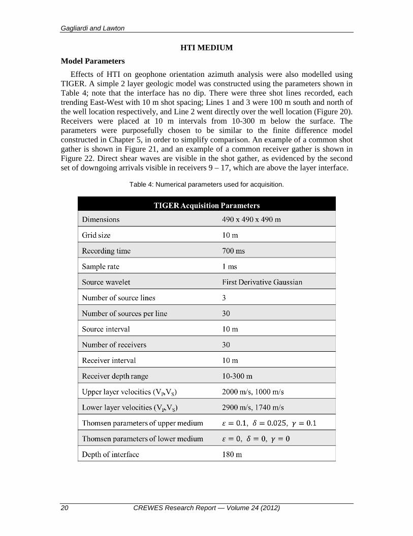
HTI MEDIUM Model Parameters

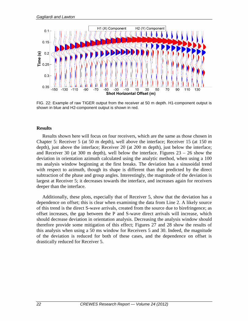
Effects of HTI on geophone orientation azimuth analysis were also modelled using TIGER. A simple 2 layer geologic model was constructed using the parameters shown in Table 4; note that the interface has no dip. There were three shot lines recorded, each trending East-West with 10 m shot spacing; Lines 1 and 3 were 100 m south and north of the well location respectively, and Line 2 went directly over the well location (Figure 20). Receivers were placed at 10 m intervals from 10-300 m below the surface. The parameters were purposefully chosen to be similar to the finite difference model constructed in Chapter 5, in order to simplify comparison. An example of a common shot gather is shown in Figure 21, and an example of a common receiver gather is shown in Figure 22. Direct shear waves are visible in the shot gather, as evidenced by the second set of downgoing arrivals visible in receivers 9 – 17, which are above the layer interface.

Table 4: Numerical parameters used for acquisition.



FIG. 20: Plan view of surface geometry used in TIGER. Line 1 is shown in blue, Line 2 is shown in black and Line 3 is shown in red.

FIG. 21: Example of raw TIGER output from the shot at x = 130 m and y = 100 m. H1-component output is shown in blue and H2-component output is shown in red.



FIG. 22: Example of raw TIGER output from the receiver at 50 m depth. H1-component output is shown in blue and H2-component output is shown in red.

Results Results shown here will focus on four receivers, which are the same as those chosen in

Chapter 5: Receiver 5 (at 50 m depth), well above the interface; Receiver 15 (at 150 m depth), just above the interface; Receiver 20 (at 200 m depth), just below the interface; and Receiver 30 (at 300 m depth), well below the interface. Figures 23 – 26 show the deviation in orientation azimuth calculated using the analytic method, when using a 100 ms analysis window beginning at the first breaks. The deviation has a sinusoidal trend with respect to azimuth, though its shape is different than that predicted by the direct subtraction of the phase and group angles. Interestingly, the magnitude of the deviation is largest at Receiver 5; it decreases towards the interface, and increases again for receivers deeper than the interface.

Additionally, these plots, especially that of Receiver 5, show that the deviation has a dependence on offset; this is clear when examining the data from Line 2. A likely source of this trend is the direct S-wave arrivals, created from the source due to birefringence; as offset increases, the gap between the P and S-wave direct arrivals will increase, which should decrease deviation in orientation analysis. Decreasing the analysis window should therefore provide some mitigation of this effect; Figures 27 and 28 show the results of this analysis when using a 50 ms window for Receivers 5 and 30. Indeed, the magnitude of the deviation is reduced for both of these cases, and the dependence on offset is drastically reduced for Receiver 5.



FIG. 23: Deviation in orientation angle for Receiver 5 (50 m depth) plotted as a function of source-well azimuth (a) and source-well offset (b). Line 1 is shown in blue, Line 2 in black and Line 3 in red.




FIG. 27: Deviation in orientation angle for Receiver 5 (50 m depth), using a 50 ms analysis window, plotted as a function of source-well azimuth (a) and source-well offset (b). Line 1 is shown in blue, Line 2 in black and Line 3 in red.

FIG. 28: Deviation in orientation angle for Receiver 30 (300 m depth), using a 50 ms analysis window, plotted as a function of source-well azimuth (a) and source-well offset (b). Line 1 is shown in blue, Line 2 in black and Line 3 in red.



Table 5 shows the standard deviation of every 5th receiver, found using both window sizes. It is also shown graphically in Figure 29 for all receivers. For receivers in the top 140 m, analysis performed using a 50 ms window shows much less scatter, again suggesting that direct S-wave arrivals have a considerable impact on this analysis. For both window sizes, there is a slight increase in scatter in the 2-3 receivers directly above the interface, which most likely arises due to contamination from reflected waves; scatter drops for the receiver located on the interface. For receivers below the interface, scatter increases with depth up to a maximum value at about 50 m below the interface, and then begins to decrease again. Note that the maximum scatter occurs at the same receiver regardless of window size.

Table 5: Standard deviation of receiver orientation azimuth.



FIG. 29: Standard deviation of orientation azimuth found using 100 ms window (a) and 50 ms window (b). The depth of the layer interface is indicated with a black line.

DISCUSSION The deviation of the well adds another level of uncertainty to this analysis; any errors

in the deviation survey will affect the analysis done for this study, although a vertical well suffers from this problem as well. Specifically, the magnitude of these uncertainties is proportional to an increased scatter in values of geophone orientation. In this case, errors of ± 2° in the inclination and azimuth of the deviation survey generally increased the scatter in orientation azimuth by about 2.5°.

The results from the dipping layer and HTI medium experiments show that calibration survey design and analysis must be guided by knowledge of the geology in the area. The modelling discussed in these sections shows that HTI anisotropy and dipping layer interfaces will produce distinct, systematic deviations in measured geophone orientation azimuth. When examining these deviations as a function of source-well azimuth, interpretable patterns may be recognised. Dipping layer interfaces will produce deviations that appear as a one-cycle sine wave that is somewhat asymmetric; deviations due to HTI anisotropy approximately match a two-cycle sine wave. It is fairly



straightforward to predict source-well azimuths that minimise these deviations: those due to dipping layer interfaces can be minimised if sources are placed along the dip direction of bedding, and those due to HTI anisotropy can be minimised if sources are placed along the slow or fast directions of geologic units. Finally, the choice of window size is shown to have an appreciable effect on the final results of the latter two analyses; this is related to contamination from turning, reflected and converted waves. Thus, it is advisable to test several analysis windows in order to produce optimal results.

CONCLUSIONS

• A simple model was created that introduced errors within ± 2° to the inclination and azimuth angles of the deviation survey; this translated to standard deviation in orientation angle of 2.53° across all 48 receiver depths, ranging from 0.06° to 13.19° for individual receivers.

• There is zero error if the source-receiver azimuth is along the maximum dip direction of the interface.

• The receivers 30 – 40 m above the velocity interface showed slight deviation, which is likely due to headwaves and reflected waves. Further, the deviation pattern as a function of source-receiver azimuth did not match that of the receivers below the interface, nor did it match the deviation predicted by raytracing.

• Deviation for receivers below the interface continued to increase with depth, reaching a maximum at 95 m below the interface when using the 50 ms window and approaching a maximum at 125 m below the interface when using the 100 ms window.

• Deviation for the receiver at 300 m found from finite difference modelling, using a 50 ms window, matched the deviation predicted by the raytracing method well.

• Deviation for receivers above the interface was consistent when using a 50 ms window, resulting in a standard deviation of approximately 2°.

• For both window sizes, deviation for receivers below the interface increased with depth, reaching a maximum at 50 m below the interface before decreasing.

• Deviation was at zero for source-receiver azimuths parallel to the fast and slow directions.

• The choice of window size was shown to be important for both the dipping layer and HTI medium. Decreasing the window size from 100 ms to 50 ms resulted in a decrease in geophone orientation deviation of over 50 % for



receivers above the interface. This is primarily due to effects from converted transmitted waves and direct S-wave arrivals.

ACKNOWLEDGEMENTS We would like to thank all CREWES Sponsors for support of this research, and

NSERC and Carbon Management Canada for additional funding.

REFERENCES Bulant, P., Eisner, L., Pšenčík, I. and Le Calvez, J., 2007, Importance of borehole deviation surveys for

monitoring of hydraulic fracturing treatments: Geophysical Prospecting, 55, 891-899. Eisner, L., Duncan, P. M., Heigl, W. M. and Keller, W. R., 2009, Uncertainties in passive seismic

monitoring: The Leading Edge, 28, 648-655. Gagliardi, P. and Lawton, D. C., Geophone azimuth consistency from calibrated vertical seismic profile

data: CREWES Research Report 23, 33.1-33.26. Le Calvez, J. H., Bennett, L., Tanner, K. V., Grant, W. D., Nutt, L., Jochen, V., Underhill, W. and Drew, J.,

2005, Monitoring microseismic fracture development to optimize stimulation and production in aging fields: The Leading Edge, 24, 72-75.

Li, X. and Yuan, J., 1999, Geophone orientation and coupling in three-component sea-floor data: a case study: Geophysical Prospecting, 47, 995-1013.

Maxwell, S. C., Rutledge, J., Jones, R. and Fehler, M., 2010, Petroleum reservoir characterization using downhole microseismic monitoring: Geophysics, 75, 75A129-75A137.

Müller, K. W., Soroka, W. L., Paulsson, B. N. P., Marmash, S., Al Baloushi, M. and Al Jeelani, O., 2010, 3D VSP technology now a standard high-resolution reservoir-imaging technique: The Leading Edge, 29, 686-697.

Refunjol, X. E., Keranen, K. M., Le Calvez, J. H. and Marfurt, K. J., 2012, Integration of hydraulically induced microseismic event locations with active seismic attributes: A North Texas Barnett Shale case study: Geophysics, 77, KS1-KS12.

Thomsen, L., 1986, Weak elastic anisotropy: Geophysics, 51, 1954-1966.

modelling of systematic errors in borehole geophone ... errors in borehole geophone orientation...

Documents