linearity, resolution, and systematic errors - nikhef
TRANSCRIPT
LINEARITY, RESOLUTION, AND
SYSTEMATIC ERRORS
of the
CCD - RASNIK
Alignment System
Gerald Dicker, NIKHEF
May – July 1997
1
Contents
1. ABSTRACT ..............................................................................................2
2. THE EFFECTIVE PIXEL SIZE ......................................................................2
2.1 Theory ...............................................................................................2
2.2 Measurement.....................................................................................4
3. CCD AND MASK PITCH VARIATIONS .........................................................6
4. A FORMULA FOR THE Z-COORDINATE .......................................................7
5. LINEARITY AND ELECTRONICALLY LIMITED PERFORMANCE.........................8
5.1 Translations.......................................................................................9
5.2 Rotations .........................................................................................10
6. THE INFLUENCE OF THE LED CURRENT ON THE RESOLUTION ...................12
7. INHOMOGENEITY OF AIR TEMPERATURE ..................................................13
7.1 The Relationship between Air Temperature and Refractive Index...13
7.2 The Bending of Light Rays in a Constant Gradient Field.................14
7.3 The RASNIK Setup with a Constant Gradient Generator ................15
7.4 Systematic Error Sources................................................................19
7.5 Random Error Increasing Sources ..................................................22
7.6 Systematic Error Decreasing...........................................................22
7.7 Random Error Decreasing: Shielding ..............................................24
8. ERROR ANALYSIS ..................................................................................35
9. CONCLUSION ........................................................................................35
10. FILES INDEX..........................................................................................36
2
1. ABSTRACT
The RASNIK - ICARAS system is examined for linearity in the translation and
rotation coordinates. A method for measuring the effective pixel size and the
distance between ccd diode array and protection glass is presented.
Resolution limiting caused by ccd / mask pitch variations, low LED current,
and air temperature gradients is discussed. Formulae for the influence of a
constant air temperature gradient on systematic measurement errors are
derived and experimental verification is given. Shielding experiments have
been carried out to study and improve the system’s performance in a heat
dissipating environment.
2. THE EFFECTIVE PIXEL SIZE
2.1 Theory
In general the effective pixel size of the ccd – frame grabber system is
different from the physical pixel size of the ccd array since the ccd camera
delivers an asynchronous signal to the frame grabber. Synchronization only
exists for the y-coordinate because the signal is sent line by line. Fast frame
grabbers improve resolution in the x direction yielding an effective pixel size
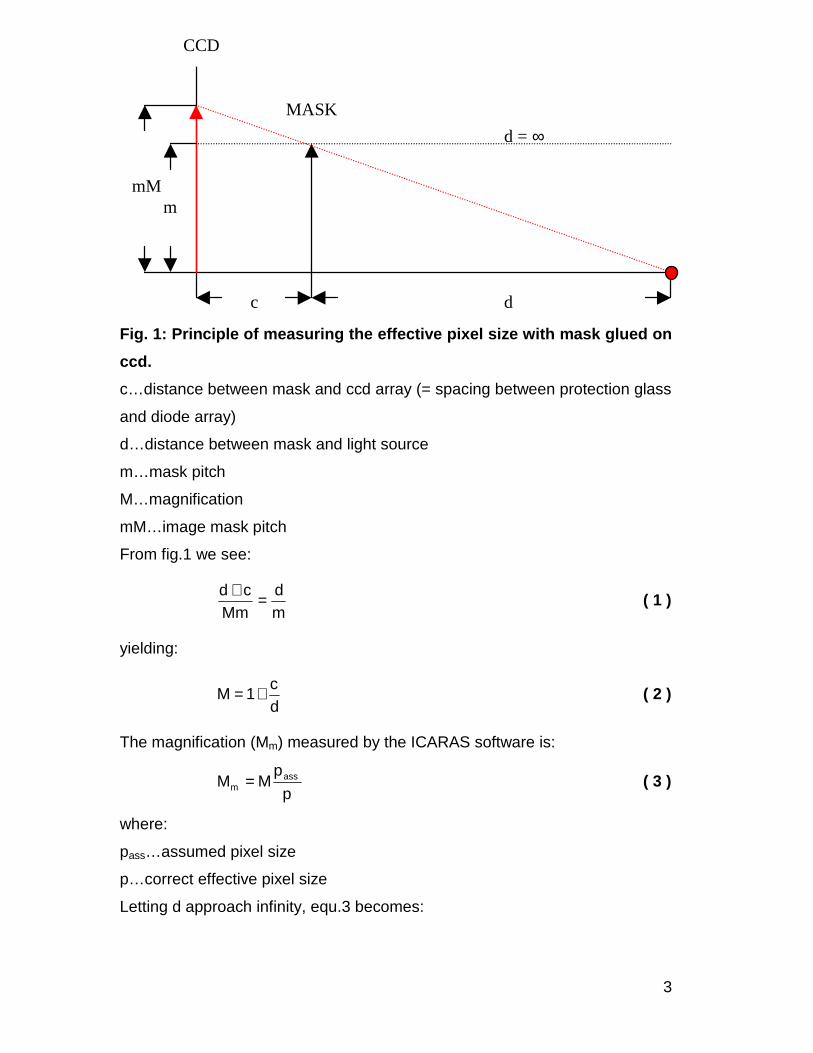
which may be smaller than the actual physical pixel size. Fig.1 depicts the
principle of measuring the effective pixel size. A piece of a RASNIK mask is
glued on the protection glass of the ccd array and illuminated by a point shape
light source. The arrow stands for one square of the mask. By making the
distance (d) of the light source infinitely large in a gedankenexperiment, the
magnification (M∞) should equal one if the effective pixel size is chosen
correct. From the deviation of M∞ from 1, we can calculate the correct
effective pixel size.
3
CCD
MASK
c d
mM m
d = ∞
Fig. 1: Principle of measuring the effective pixel size with mask glued on
ccd.
c…distance between mask and ccd array (= spacing between protection glass
and diode array)
d…distance between mask and light source
m…mask pitch
M…magnification
mM…image mask pitch
From fig.1 we see:
md
Mmcd =+
( 1 )
yielding:
dc
1M += ( 2 )
The magnification (Mm) measured by the ICARAS software is:
p
pMM ass
m = ( 3 )
where:
pass…assumed pixel size
p…correct effective pixel size
Letting d approach infinity, equ.3 becomes:
4
p
pM)d(M ass
m ==∞= ∞ ( 4 )
∞
=M
pp ass ( 5 )
Equ.3 multiplied with d gives a linear function in d.
∞∞ += cMdMdMm ( 6 )
If (Mm d) is plotted versus d, a linear fit will reveal M∞ as the slope and (c M∞)
as the intercept of this curve.
∞
=Merceptint
c ( 7 )
The effective pixel size can be calculated via equ.5.
2.2 Measurement
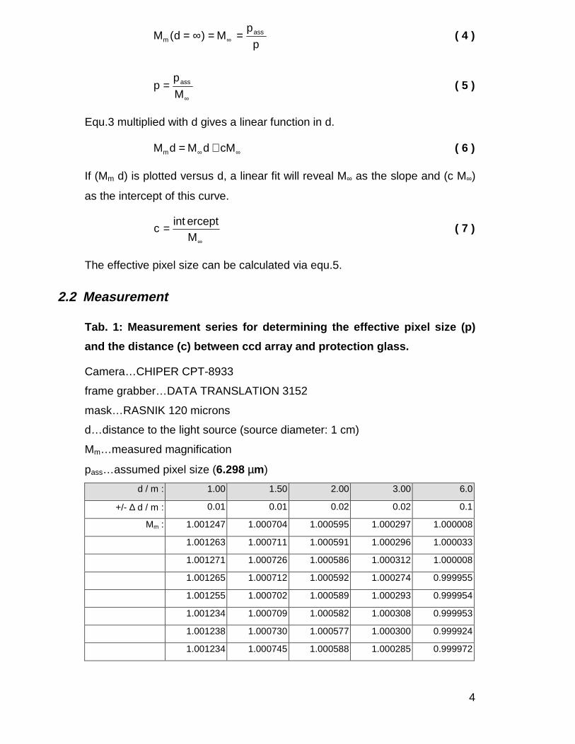
Tab. 1: Measurement series for determining the effective pixel size (p)
and the distance (c) between ccd array and protection glass.
Camera…CHIPER CPT-8933
frame grabber…DATA TRANSLATION 3152
mask…RASNIK 120 microns
d…distance to the light source (source diameter: 1 cm)
Mm…measured magnification
pass…assumed pixel size (6.298 µm)
d / m : 1.00 1.50 2.00 3.00 6.0
+/- ∆ d / m : 0.01 0.01 0.02 0.02 0.1
Mm : 1.001247 1.000704 1.000595 1.000297 1.000008
1.001263 1.000711 1.000591 1.000296 1.000033
1.001271 1.000726 1.000586 1.000312 1.000008
1.001265 1.000712 1.000592 1.000274 0.999955
1.001255 1.000702 1.000589 1.000293 0.999954
1.001234 1.000709 1.000582 1.000308 0.999953
1.001238 1.000730 1.000577 1.000300 0.999924
1.001234 1.000745 1.000588 1.000285 0.999972
5
1.001230 1.000726 1.000586 1.000275 0.999829
1.001221 1.000704 1.000582 1.000292 1.000013
average : 1.001246 1.000717 1.000587 1.000293 0.999965
rms : 0.000017 0.000014 0.000005 0.000013 0.000059
Mm d / m : 1.001 1.501 2.001 3.001 6.00
+/- ∆ (Mm d) / m : 0.010 0.010 0.020 0.020 0.10
0.9996
0.9998
1.0000
1.0002
1.0004
1.0006
1.0008
1.0010
1.0012
1.0014
1.0016
0.00 1.00 2.00 3.00 4.00 5.00 6.00 7.00
d / m
mag
nific
atio
n
measuredtheoret. curveM (infinity)
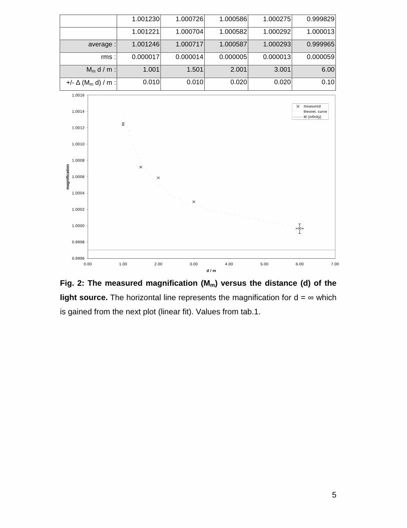
Fig. 2: The measured magnification (M m) versus the distance (d) of the
light source. The horizontal line represents the magnification for d = ∞ which
is gained from the next plot (linear fit). Values from tab.1.
6
Mmd = 0.9997d + 0.0016
0.00
1.00
2.00
3.00
4.00
5.00
6.00
7.00
0.00 1.00 2.00 3.00 4.00 5.00 6.00 7.00
d / m
Mm
d /
m
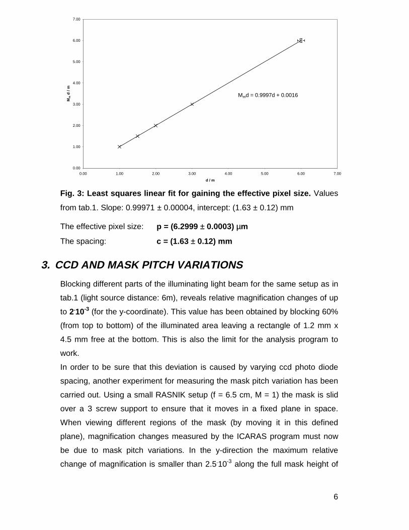
Fig. 3: Least squares linear fit for gaining the effective pixel size. Values
from tab.1. Slope: 0.99971 ± 0.00004, intercept: (1.63 ± 0.12) mm
The effective pixel size: p = (6.2999 ± 0.0003) µm
The spacing: c = (1.63 ± 0.12) mm
3. CCD AND MASK PITCH VARIATIONS
Blocking different parts of the illuminating light beam for the same setup as in
tab.1 (light source distance: 6m), reveals relative magnification changes of up
to 2.10-3 (for the y-coordinate). This value has been obtained by blocking 60%
(from top to bottom) of the illuminated area leaving a rectangle of 1.2 mm x
4.5 mm free at the bottom. This is also the limit for the analysis program to
work.
In order to be sure that this deviation is caused by varying ccd photo diode
spacing, another experiment for measuring the mask pitch variation has been
carried out. Using a small RASNIK setup (f = 6.5 cm, M = 1) the mask is slid
over a 3 screw support to ensure that it moves in a fixed plane in space.
When viewing different regions of the mask (by moving it in this defined
plane), magnification changes measured by the ICARAS program must now
be due to mask pitch variations. In the y-direction the maximum relative
change of magnification is smaller than 2.5.10-3 along the full mask height of
7
20 mm, i.e. a variation of 1.5.10-4 within 1.2 mm which is (almost) negligible
compared to 2.10-3. In other words, the magnification changes measured
above are due to ccd diode size (or spacing) variations. Hence, the mask
pitch variation measured in the y direction is ± 0.3 microns . The maximum
relative change of magnification in x measured is 5.6.10-4 yielding a mask
pitch variation of ± 0.07 microns .
The ccd errors do not significantly influence the measurements of x, y, and rot
z when the whole array is illuminated. The case is different for the out of plane
rotations rot x and rot y where errors will occur.
4. A FORMULA FOR THE Z-COORDINATE
In the following equations the distance between ccd and lens (= b) is assumed
to be constant. The calculations refer to displacements of the mask. The
distance between mask and lens (= g) is:
Mb
g = ( 8 )
where M is the magnification.
A conventional definition of the z-coordinate assigns z = 0 to the situation
where the imaging equation is fulfilled,
0g1
b1
f1 += ( 9 )
where f is the focal length. With the usual sign convention we get:
Mb
gggz 00 −=−= ( 10 )
It is not easy to measure b with micron precision. An alternative formulation
for the z-coordinate, which does not require a measurement of b but a sharp
image on the screen, can be obtained as follows.
)M1
M1
(bz0
−= ( 11 )
)1M(fb 0 += ( 12 )

8
)M1
M1
)(1M(fz0
0 −+= ( 13 )
M0 refers to the initial situation where the imaging equation is fulfilled (= sharp
image).
5. LINEARITY AND ELECTRONICALLY LIMITED
PERFORMANCE
Due to a damage of the frame grabber (DATA TRANSLATION 3152) it has
had to be exchanged. The effective pixel size of the “new” one (MATRIX
VISION, PC process M, MGVS module) in combination with the ccd camera
(CHIPER CPT-8933) is measured to be:
p = (6.297 ± 0.001) µm
A slightly different method than described above is employed for the
measurement: The ccd, with the piece of mask glued on it, is illuminated by
parallel light which has been produced by means of autocollimation.
In order to measure the ultimate i.e. electronically limited performance, a
small setup (called “mini”) with a lens (MELLES GRIOT 01LDX125) of short
focal length (f = 63.5 mm, D = 40 mm) is used. With a short light path through
the air, temperature effects can practically be excluded. It has turned out that
the spherical aberrations of the lens cause the image to turn gray and the
ICARAS software to fail. As a consequence the lens diameter has been
decreased to 20 mm by using a diaphragm of black paper reducing the
influence of the wrong curvature of the outer lens region. The setup is used in
the symmetrical (M = 1, b = g = 2f) situation. For producing well defined three
dimensional displacements, a high-precision mount (NEWPORT M-460A)
driven by three micrometer screws is used. Rotations are carried out with a
rotating mount (M-TGN80). A uniform illumination of the mask is met by using
nine infrared LEDs and a ground glass plate. In the following diagrams the
errors of the RASNIK measured values are gained from the standard
deviation of ten measurements. A least squares linear approximation yields
the slope of the plotted trendlines.
9
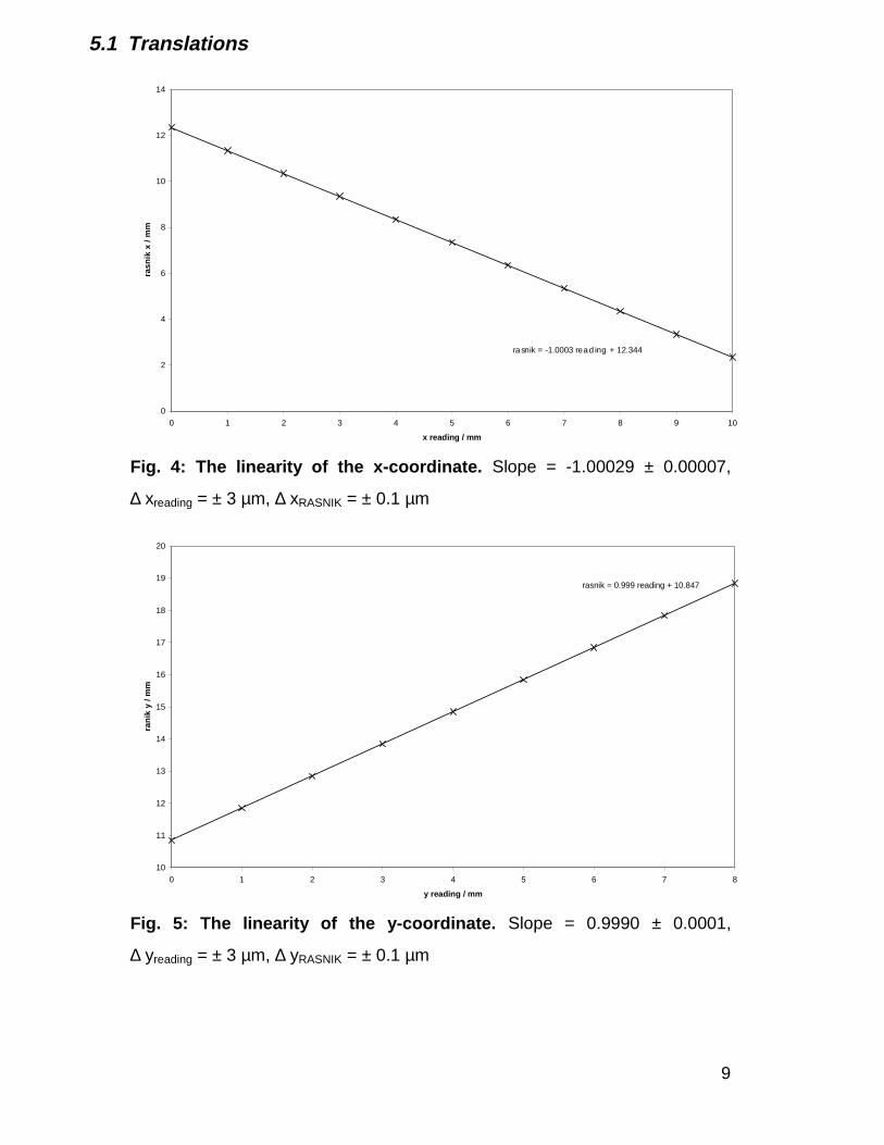
5.1 Translations
rasnik = -1.0003 reading + 12.344
0
2
4
6
8
10
12
14
0 1 2 3 4 5 6 7 8 9 10
x reading / mm
rasn
ik x
/ m
m
Fig. 4: The linearity of the x-coordinate. Slope = -1.00029 ± 0.00007,
∆ xreading = ± 3 µm, ∆ xRASNIK = ± 0.1 µm
rasnik = 0.999 reading + 10.847
10
11
12
13
14
15
16
17
18
19
20
0 1 2 3 4 5 6 7 8
y reading / mm
rani
k y
/ mm
Fig. 5: The linearity of the y-coordinate. Slope = 0.9990 ± 0.0001,
∆ yreading = ± 3 µm, ∆ yRASNIK = ± 0.1 µm
10
rasnik = -0.9971 reading + 4.3123
-1.5
-1
-0.5
0
0.5
1
1.5
2
2.5
2 2.5 3 3.5 4 4.5 5 5.5 6
z reading / mm
rasn
ik z
/ m
m
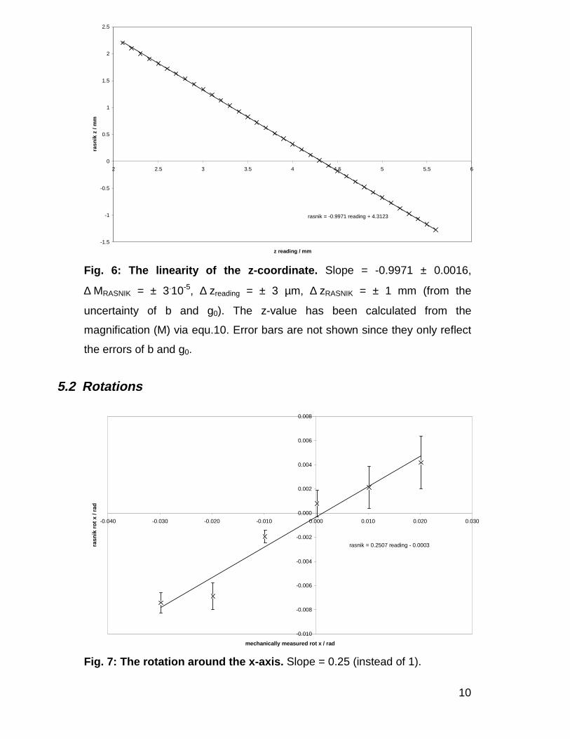
Fig. 6: The linearity of the z-coordinate. Slope = -0.9971 ± 0.0016,
∆ MRASNIK = ± 3.10-5, ∆ zreading = ± 3 µm, ∆ zRASNIK = ± 1 mm (from the
uncertainty of b and g0). The z-value has been calculated from the
magnification (M) via equ.10. Error bars are not shown since they only reflect
the errors of b and g0.
5.2 Rotations
rasnik = 0.2507 reading - 0.0003
-0.010
-0.008
-0.006
-0.004
-0.002
0.000
0.002
0.004
0.006
0.008
-0.040 -0.030 -0.020 -0.010 0.000 0.010 0.020 0.030
mechanically measured rot x / rad
rasn
ik r
ot x
/ ra
d
Fig. 7: The rotation around the x-axis. Slope = 0.25 (instead of 1).

11
rasnik = 0.3515 reading - 3E-07
-0.02
-0.01
-0.01
0.00
0.01
0.01
0.02
0.02
0.03
-0.04 -0.03 -0.02 -0.01 0.00 0.01 0.02 0.03
mechanically measured angle / rad
rasn
ik r
ot y
/ ra
d
Fig. 8: The rotation around the y-axis. Slope = 0.35 (instead of 1).
Additional problems with measuring the out-of-plane rotations rot x and rot y
might arise from the ccd pitch variations as stated in chapter 3.
y = 0.9995x + 1E-05
-0.04
-0.02
0.00
0.02
0.04
0.06
0.08
-0.04 -0.02 0.00 0.02 0.04 0.06 0.08
mechanically measured rot z / rad
rasn
ik r
ot z
/ ra
d
Fig. 9: The rotation around the z-axis. Slope = 0.9996 ± 0.0002,
∆ (rot z)reading = 0.3 mrad, ∆ (rot z)RASNIK = 0.02 mrad
12
6. THE INFLUENCE OF THE LED CURRENT ON THE
RESOLUTION
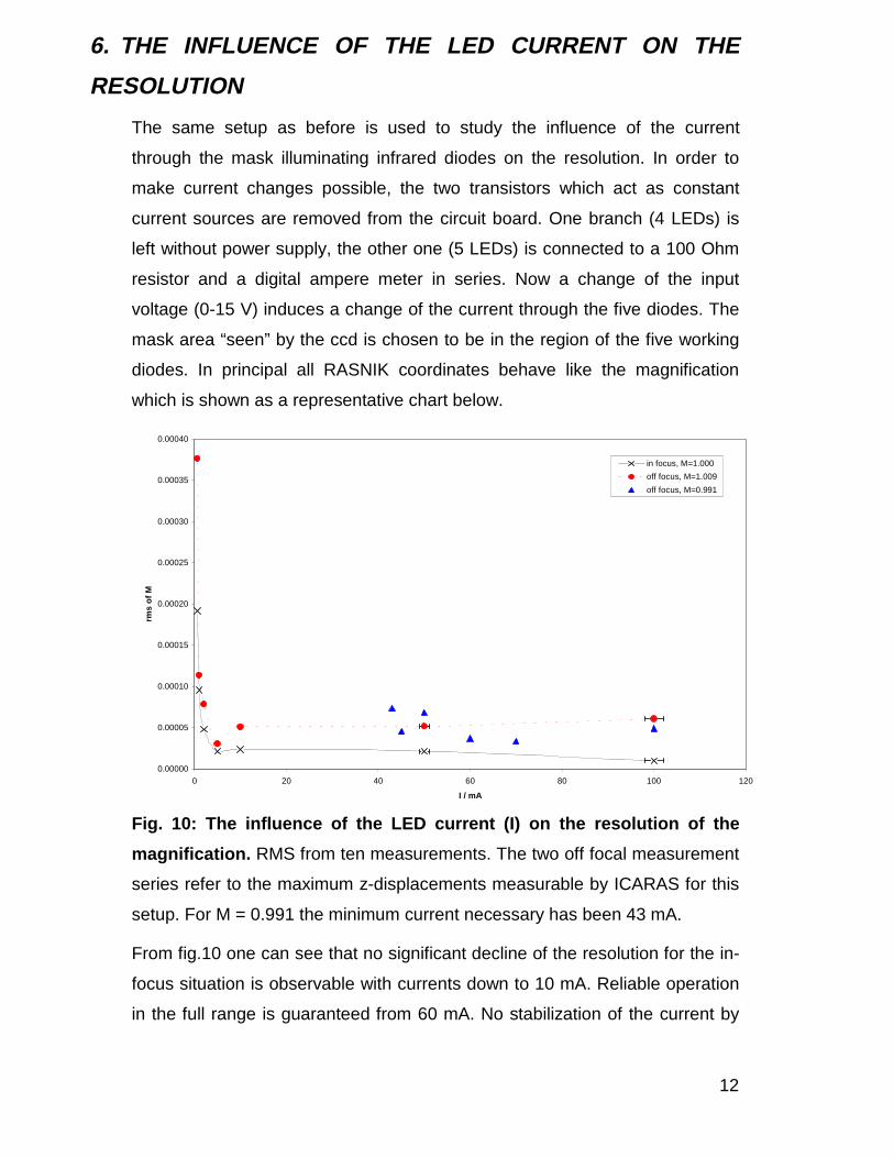
The same setup as before is used to study the influence of the current
through the mask illuminating infrared diodes on the resolution. In order to
make current changes possible, the two transistors which act as constant
current sources are removed from the circuit board. One branch (4 LEDs) is
left without power supply, the other one (5 LEDs) is connected to a 100 Ohm
resistor and a digital ampere meter in series. Now a change of the input
voltage (0-15 V) induces a change of the current through the five diodes. The
mask area “seen” by the ccd is chosen to be in the region of the five working
diodes. In principal all RASNIK coordinates behave like the magnification
which is shown as a representative chart below.
0.00000
0.00005
0.00010
0.00015
0.00020
0.00025
0.00030
0.00035
0.00040
0 20 40 60 80 100 120
I / mA
rms
of M
in focus, M=1.000
off focus, M=1.009
off focus, M=0.991
Fig. 10: The influence of the LED current (I) on the resolution of the
magnification. RMS from ten measurements. The two off focal measurement
series refer to the maximum z-displacements measurable by ICARAS for this
setup. For M = 0.991 the minimum current necessary has been 43 mA.
From fig.10 one can see that no significant decline of the resolution for the in-
focus situation is observable with currents down to 10 mA. Reliable operation
in the full range is guaranteed from 60 mA. No stabilization of the current by
13
means of transistors is needed. In large setups a condenser lens replaces the
ground glass plate to ensure uniform illumination.
7. INHOMOGENEITY OF AIR TEMPERATURE
7.1 The Relationship between Air Temperature and Refractive
Index
An empirical formula for the dependence of the refractive index of air on the
temperature at a pressure of 760 Torr and at a wavelength of 850 nm is
used1:
t1
nn 0
t α+∆
=∆ ( 14 )
with: ∆n0 = 2895 10-7
α = 0.003672 (oC)-1
where:
∆nt …the difference of the refractive index to vacuum
∆n0 …the difference of the refractive index to vacuum at t = 0 oC
t …temperature in oC
Expanding this expression into a power series around t = 20 oC and
neglecting higher order terms yields:
O)201(
)20t(n
201
nn
200
t +α+−α∆
−α+
∆≈∆ ( 15 )
With this linear expression one can easily calculate a constant gradient (K)
between two points of different temperatures (tt and tb) separated by a
distance h. The letters t, b, and h refer to top, bottom, and height,
respectively, for reasons of clearness.
1 Robert C. Weast (editor), Handbook of Chemistry and Physics, Chemical
Rubber Publishing Company, 58th ed., p. E224

14
)tt()201(h
nK tb2
0 −α+
α∆= ( 16 )
7.2 The Bending of Light Rays in a Constant Gradient Field
In geometrical optics light propagating through a medium is described in
terms of light rays. In a medium of homogeneous refractive index these rays
are straight lines. The differential equation of light rays is given by2:
nds
rdn
dsd ∇=
&
&
( 17 )
where:
s …length of the ray measured from a fixed point on it
r&
…position vector
n …refractive index
We want to limit our considerations on two dimensions and furthermore make
the following assumptions:
1. Constant gradient of the refractive index in the y direction: yeK:n&
&
⋅=∇
2. The light ray initially travels parallel to the x-axis.
3. For “small” deviations of the light beam from the initial horizontal direction
we may assume 0dsdn ≈ , hence n)s(n = .
We obtain the following system which is easily solved.
0ds
xd2
2
= ( 18 )
Kds
ydn
2
2
= ( 19 )
If the origin of the light ray and the one of our coordinate system coincide, we
get the following trajectory in parametric form.
sx = ( 20 )
2 Max Born and Emil Wolf, Principles of Optics, Pergamon Press, 6th ed.,
p.122

15
n2Ks
y2
= ( 21 )
The result is a quadratic deviation from the straight line with the light ray
bending towards the region of higher refractive index.
n2Kx
)x(y2
= ( 22 )
7.3 The RASNIK Setup with a Constant Gradient Generator
7.3.1 Experimental Arrangement
For studying the air temperature influence, a large RASNIK setup (called
“big”) with a total length of 7.18 meters is used. The mask pitch in this setup is
170 µm, the lens diameter (D) 45 mm. A constant gradient generator is
realized as follows. An aluminum tube with rectangular cross section is heated
with heating ropes at its top (see fig.11). Either end of the hollow bar is
covered with a transparent foil to minimize air convection. There are two
principal arrangements for testing the influence of a constant gradient
generator on the RASNIK system. The generator can be placed either
between lens and ccd (fig.12) or between mask and lens (fig.13).
hl
Fig. 11: The constant gradient generator.
h = (100 ± 1) mm, l = (1000 ± 1) mm.
16
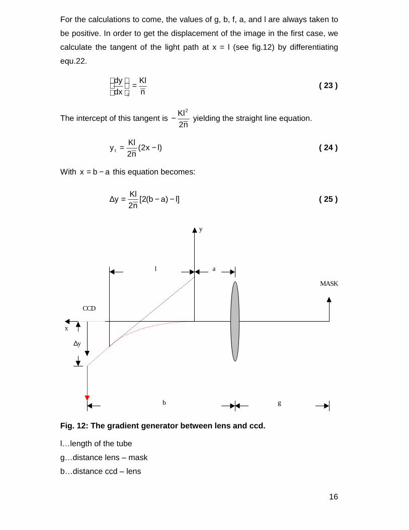
For the calculations to come, the values of g, b, f, a, and l are always taken to
be positive. In order to get the displacement of the image in the first case, we
calculate the tangent of the light path at x = l (see fig.12) by differentiating
equ.22.
nKl
dxdy
l
=
( 23 )
The intercept of this tangent is n2
Kl2
− yielding the straight line equation.
)lx2(n2
Kly t −= ( 24 )
With abx −= this equation becomes:
]l)ab(2[n2
Kly −−=∆ ( 25 )
MASK
CCD
y
x
l a
b g
∆y
Fig. 12: The gradient generator between lens and ccd.
l…length of the tube
g…distance lens – mask
b…distance ccd – lens
17
a…distance between tube and lens
∆y…image displacement due to the temperature gradient
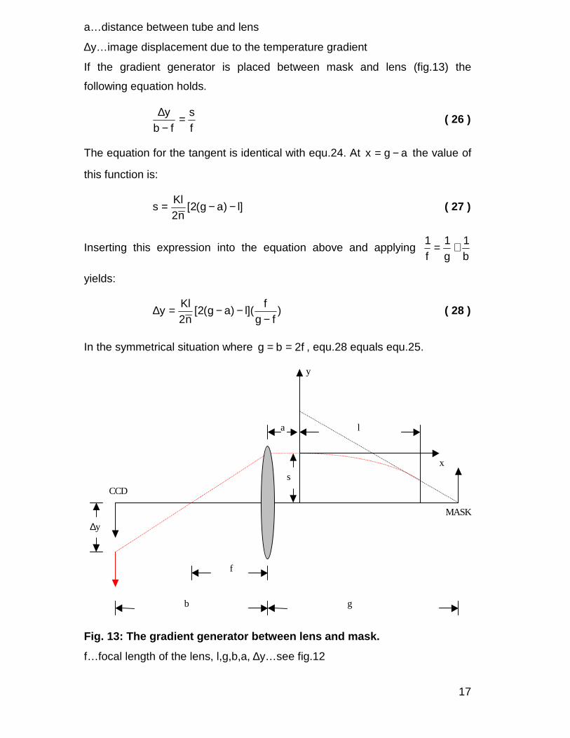
If the gradient generator is placed between mask and lens (fig.13) the
following equation holds.
fs
fby =−
∆ ( 26 )
The equation for the tangent is identical with equ.24. At agx −= the value of
this function is:
]l)ag(2[n2
Kls −−= ( 27 )
Inserting this expression into the equation above and applying b1
g1
f1 +=
yields:
)fg
f](l)ag(2[
n2Kl
y−
−−=∆ ( 28 )
In the symmetrical situation where f2bg == , equ.28 equals equ.25.
MASK
CCD
y
x
a l
b g
f
s
∆y
Fig. 13: The gradient generator between lens and mask.
f…focal length of the lens, l,g,b,a, ∆y…see fig.12
18
7.3.2 Measurements
The Rasnik y value is measured after heating the tube for at least 20 minutes
when a stable gradient is achieved. The value measured before heating is
then subtracted from it. The error is gained by the rms of ten consecutive
measurements taking the subtraction into account. The temperatures are
measured with sensors wrapped round with aluminum foil and glued on the
bar with a sticky tape. The top temperature is measured by three digital
sensors distributed on the roof, the bottom one with two sensors (one did not
work properly). The measurement error of one sensor is indicated to be ±1 oC.
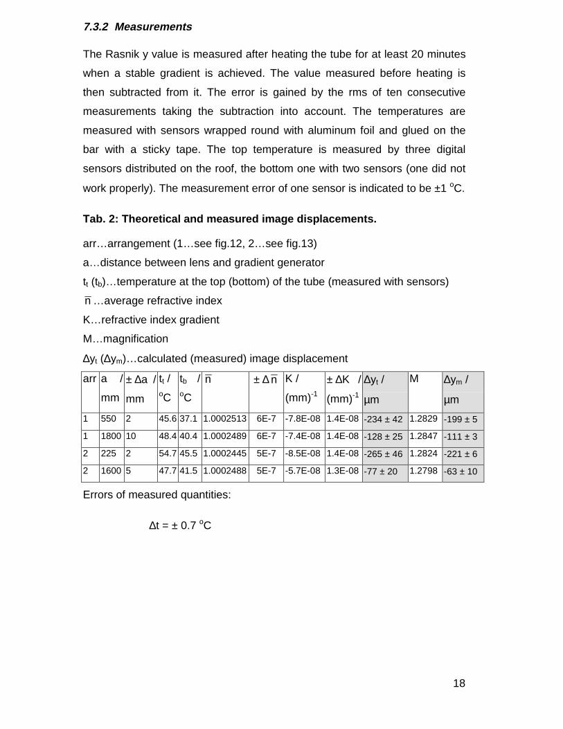
Tab. 2: Theoretical and measured image displacements.
arr…arrangement (1…see fig.12, 2…see fig.13)
a…distance between lens and gradient generator
tt (tb)…temperature at the top (bottom) of the tube (measured with sensors)
n …average refractive index
K…refractive index gradient
M…magnification
∆yt (∆ym)…calculated (measured) image displacement
arr a /
mm
± ∆a /
mm
tt /oC
tb /oC
n ± ∆ n K /
(mm)-1
± ∆K /
(mm)-1
∆yt /
µm
M ∆ym /
µm
1 550 2 45.6 37.1 1.0002513 6E-7 -7.8E-08 1.4E-08 -234 ± 42 1.2829 -199 ± 5
1 1800 10 48.4 40.4 1.0002489 6E-7 -7.4E-08 1.4E-08 -128 ± 25 1.2847 -111 ± 3
2 225 2 54.7 45.5 1.0002445 5E-7 -8.5E-08 1.4E-08 -265 ± 46 1.2824 -221 ± 6
2 1600 5 47.7 41.5 1.0002488 5E-7 -5.7E-08 1.3E-08 -77 ± 20 1.2798 -63 ± 10
Errors of measured quantities:
∆t = ± 0.7 oC
19
Formulae:
∆ym = ∆yRASNIK . M 3
K…equ.16
∆yt…equs.25,28
t1
n1n 0
α+∆
+= ( 29 )
t = (tt + tb) / 2 ( 30 )
with:
f = 1774 mm g = (3150 ± 10) mm
b = (4030 ± 10) mm h = (100 ± 1) mm
l = (1000 ± 1) mm ∆n0, α…see equ.14
The systematic deviations of the measured image displacements from the
theoretically predicted ones in tab.2 are all within the error tolerance.
However, they are 16 % lower on average which may be interpreted as
systematical. This indicates that the gradient is not constant as assumed or
about 16 % systematically lower than calculated. From shielding experiments
the former assumption seems quite appropriate for one can see there that the
vertical gradient within a common shield, i.e. a shield with top, bottom, and
side shields, is larger close to the top and smaller close to the bottom of the
shield. The light beam in this experiment has passed the gradient generator
close to the bottom.
7.4 Systematic Error Sources
Heat sources close above the light beam mainly induce systematic errors
whereas heating below the axis merely induces an increase of the random
error. In the latter case one might expect an upward bending of light rays. This
3 The measured RASNIK value ∆yRASNIK has to be multiplied with the
magnification (M) because the ICARAS software gives the displacement in
terms of the mask displacement but not the actual displacement of the image.

20
is not the case since the generation of a stable temperature gradient is always
disturbed by the ascent of warm air from the heat source below yielding a
blurring of the image (high random error) rather than a systematical
displacement. The influence of the gradient on the image displacement is
linear with its distance from the ccd or the mask, respectively (see equs.25,
28, and figs.12, 13). The closer the heat source is to the lens the larger errors
occur. In the following plots the systematic error is obtained through averaging
over ten consecutive measurements and subtracting this value from the
averaged value of ten measurements without heating (negative time). In order
to measure a reliable random error (= standard deviation of ten consecutive
measurements) the heat capacity of the studied sources has to be large
enough, so that the temperature within ten measurements (for obtaining the
random error) can be assumed constant.
-50
-40
-30
-20
-10
0
10
20
30
-200 0 200 400 600 800 1000 1200 1400 1600 1800
heating time / s
∆y /
µm
systematic error
random error
Fig. 14: Aluminum sheet as systematic error source. The sheet
(thickness: 1.5 mm) is heated with a heating rope lying on it and is placed
close (3 cm) above the optical axis. The distance of one edge to the lens is
about 20 cm and the light beam is influenced on a length of 59 cm.
21
-180
-160
-140
-120
-100
-80
-60
-40
-20
0
20
0 500 1000 1500 2000 2500 3000 3500 4000 4500
heating time of tube / s
∆ y
/ µm
random error
systematic error
high rms due to rapid systematic change of y value
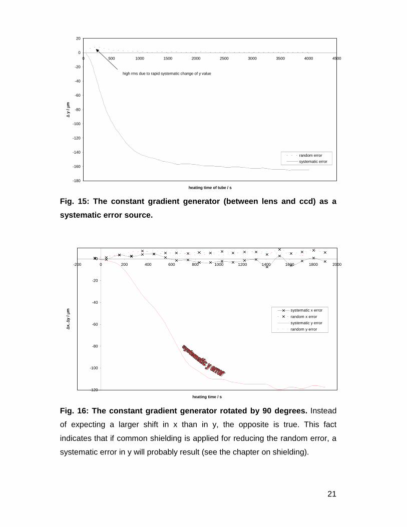
Fig. 15: The constant gradient generator (between lens and ccd) as a
systematic error source.
-120
-100
-80
-60
-40
-20
0-200 0 200 400 600 800 1000 1200 1400 1600 1800 2000
heating time / s
∆x,
∆y /
µm
systematic x error
random x error
systematic y error
random y error
Fig. 16: The constant gradient generator rotated by 90 degrees. Instead
of expecting a larger shift in x than in y, the opposite is true. This fact
indicates that if common shielding is applied for reducing the random error, a
systematic error in y will probably result (see the chapter on shielding).

22
7.5 Random Error Increasing Sources
In the experiments carried out no systematic error has been observed when
placing a heat source below the light beam. Fig.17 serves as an example for
random error increase.
-10
-5
0
5
10
15
20
-200 0 200 400 600 800 1000 1200 1400 1600 1800
heating time / s
∆y /
µm
random error
systematic error
Fig. 17: Aluminum box filled with a heating rope as a random error
increasing source. The heat source is placed about 1 m below the axis and
1.5 m away from the lens. Box dimensions: 23 x 20 x 10 cm3, 3 mm thick
body.
7.6 Systematic Error Decreasing
In all the following experiments the same heat source as mentioned in Fig.17
has been used. In order to reduce systematic errors one has to take care that
the medium (air) the beam passes through is in random movement. This can
be achieved e.g. through circulating the air by means of ventilators. As will be
seen later, shields of the common type (with top, bottom, and side shields)
may cause systematic errors which can be reduced by blowing air through
them. Fig.18 depicts an example of systematic error decrease by applying the
latter technique.
23
-10
-8
-6
-4
-2
0
2
4
6
-500 0 500 1000 1500 2000 2500 3000 3500 4000 4500
heating time / s
∆y /
µm
systematic errorrandom errorsys. err. with vent.rand. err. with vent.
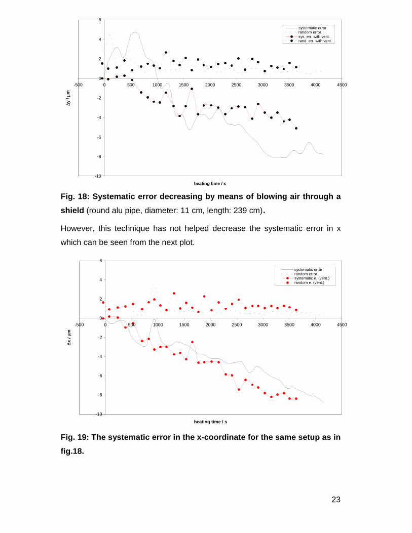
Fig. 18: Systematic error decreasing by means of blowing air through a
shield (round alu pipe, diameter: 11 cm, length: 239 cm).
However, this technique has not helped decrease the systematic error in x
which can be seen from the next plot.
-10
-8
-6
-4
-2
0
2
4
6
-500 0 500 1000 1500 2000 2500 3000 3500 4000 4500
heating time / s
∆x /
µm
systematic errorrandom errorsystematic e. (vent.)random e. (vent.)
Fig. 19: The systematic error in the x-coordinate for the same setup as in
fig.18.

24
7.7 Random Error Decreasing: Shielding
Whenever large fluctuations of the refractive index due to a heat source below
the optical axis occur, shielding of the beam is required to minimize random
errors. In the following chapters a round aluminum pipe as mentioned above
and a shield, also made of aluminum, with a cross section of the shape of an
isosceles triangle with a right angle are used. The baseline of this triangle is
26.5 cm and the thickness of the sheets is 1 mm. The shield is 150 cm long.
The triangular shield is used in two different ways. It is used with the baseline
on the bottom (∆, upright) or turned around by 180o resembling a “give way” –
traffic sign (∇ , gws). Each setup is tested with the light beam passing near
the top and the bottom of the shield. In order to evaluate the absolute
effectiveness of each shield, the deviations of the Rasnik values when no
shielding is applied are depicted in the chapter: The Flat Sheet.

25
7.7.1 The X-Coordinate
0
2
4
6
8
10
12
-500 0 500 1000 1500 2000 2500 3000 3500 4000 4500 5000
heating time / s
∆x /
µm
random (upright)
random (gws)
random (round)
-16
-14
-12
-10
-8
-6
-4
-2
0
2
4
-500 0 500 1000 1500 2000 2500 3000 3500 4000 4500 5000
heating time / s
∆x /
µm
systematic (gws)
systematic (upright)
systematic (round)
Fig. 20: Random and systematic errors with different shields. Beam
passes at the top.

26
0
2
4
6
8
10
12
-500 0 500 1000 1500 2000 2500 3000 3500 4000 4500 5000
heating time / s
∆x /
µm
random (upright)
random (gws)
random (round)
-16
-14
-12
-10
-8
-6
-4
-2
0
2
4
-500 0 500 1000 1500 2000 2500 3000 3500 4000 4500 5000
heating time / s
∆x /
µm
systematic (upright)
systematic (gws)systematic (round)
Fig. 21: Random and systematic errors with different shields. Beam
passes at the bottom.
27
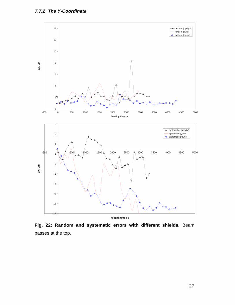
7.7.2 The Y-Coordinate
0
2
4
6
8
10
12
14
-500 0 500 1000 1500 2000 2500 3000 3500 4000 4500 5000
heating time / s
∆y /
µm
random (upright)
random (gws)
random (round)
-13
-11
-9
-7
-5
-3
-1
1
3
5
-500 0 500 1000 1500 2000 2500 3000 3500 4000 4500 5000
heating time / s
∆y /
µm
systematic (upright)
systematic (gws)
systematic (round)
Fig. 22: Random and systematic errors with different shields. Beam
passes at the top.
28
0
2
4
6
8
10
12
14
-500 0 500 1000 1500 2000 2500 3000 3500 4000 4500 5000
heating time / s
∆y /
µm
random (upright)
random (gws)
random (round)
-13
-11
-9
-7
-5
-3
-1
1
3
5
-500 0 500 1000 1500 2000 2500 3000 3500 4000 4500 5000
heating time / s
∆y /
µm
systematic (upright)
systematic (gws)
systematic (round)
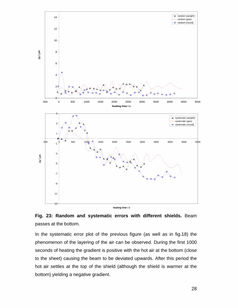
Fig. 23: Random and systematic errors with different shields. Beam
passes at the bottom.
In the systematic error plot of the previous figure (as well as in fig.18) the
phenomenon of the layering of the air can be observed. During the first 1000
seconds of heating the gradient is positive with the hot air at the bottom (close
to the sheet) causing the beam to be deviated upwards. After this period the
hot air settles at the top of the shield (although the shield is warmer at the
bottom) yielding a negative gradient.
29
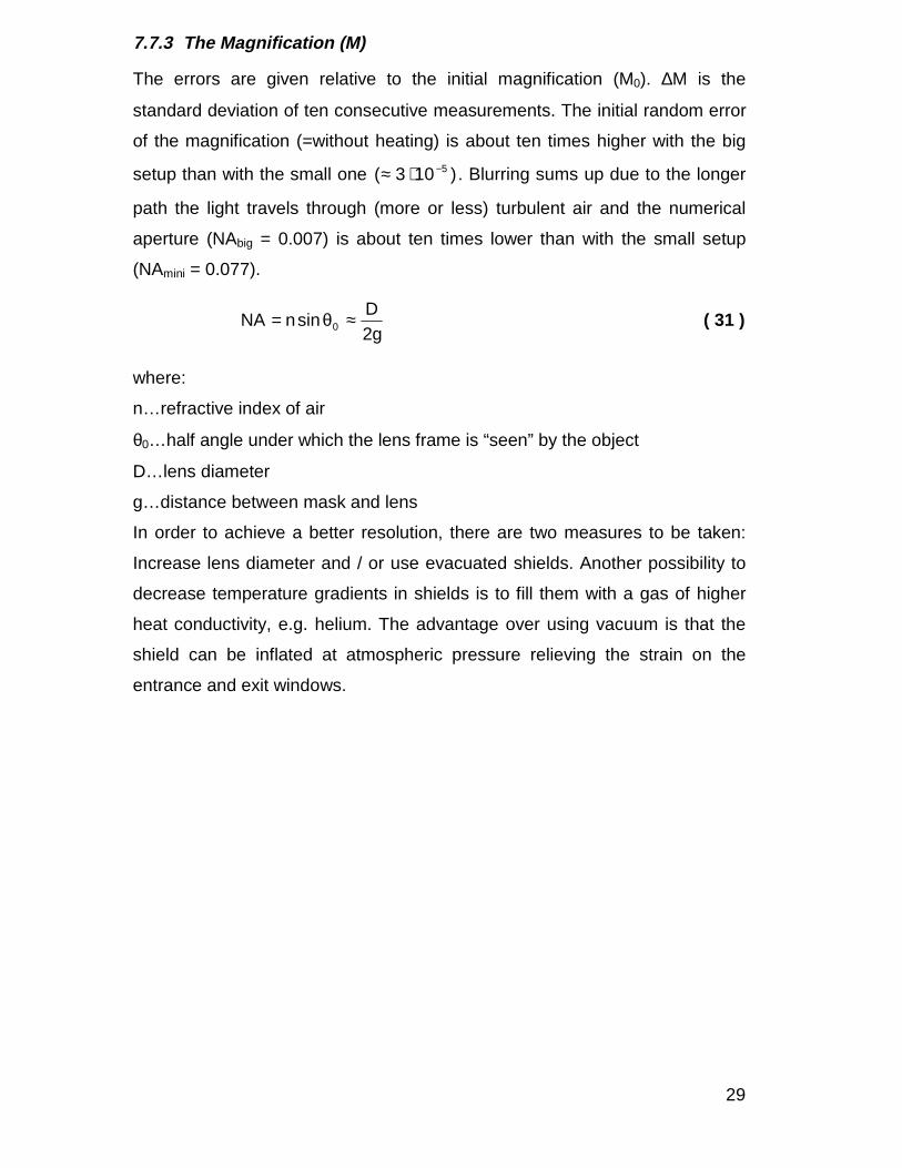
7.7.3 The Magnification (M)
The errors are given relative to the initial magnification (M0). ∆M is the
standard deviation of ten consecutive measurements. The initial random error
of the magnification (=without heating) is about ten times higher with the big
setup than with the small one )103( 5−⋅≈ . Blurring sums up due to the longer
path the light travels through (more or less) turbulent air and the numerical
aperture (NAbig = 0.007) is about ten times lower than with the small setup
(NAmini = 0.077).
g2D
sinnNA 0 ≈θ= ( 31 )
where:
n…refractive index of air
θ0…half angle under which the lens frame is “seen” by the object
D…lens diameter
g…distance between mask and lens
In order to achieve a better resolution, there are two measures to be taken:
Increase lens diameter and / or use evacuated shields. Another possibility to
decrease temperature gradients in shields is to fill them with a gas of higher
heat conductivity, e.g. helium. The advantage over using vacuum is that the
shield can be inflated at atmospheric pressure relieving the strain on the
entrance and exit windows.
30
0.0000
0.0001
0.0002
0.0003
0.0004
0.0005
0.0006
0.0007
0.0008
0.0009
0.0010
-500 0 500 1000 1500 2000 2500 3000 3500 4000 4500 5000
heating time / s
∆M /
M0
random (upright)
random (round)
random (gws)
-0.0005
-0.0003
-0.0001
0.0001
0.0003
0.0005
0.0007
0.0009
0.0011
-500 0 500 1000 1500 2000 2500 3000 3500 4000 4500 5000
heating time / s
M /
M0
- 1
systematic (upright)
systematic (gws)
systematic (round)
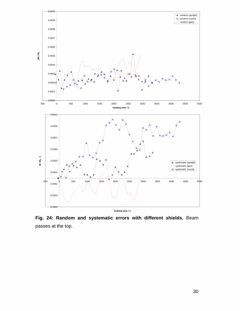
Fig. 24: Random and systematic errors with different shields. Beam
passes at the top.
31
0.0000
0.0001
0.0002
0.0003
0.0004
0.0005
0.0006
0.0007
0.0008
0.0009
0.0010
-500 0 500 1000 1500 2000 2500 3000 3500 4000 4500 5000
heating time / s
∆M /
M0
random (upright)
random (gws)
random (round)
-0.0005
-0.0003
-0.0001
0.0001
0.0003
0.0005
0.0007
0.0009
0.0011
-500 0 500 1000 1500 2000 2500 3000 3500 4000 4500 5000
heating time / s
M /
M0
- 1
systematic (upright)
systematic (gws)
systematic (round)
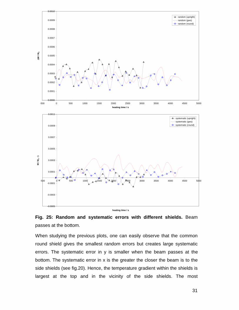
Fig. 25: Random and systematic errors with different shields. Beam
passes at the bottom.
When studying the previous plots, one can easily observe that the common
round shield gives the smallest random errors but creates large systematic
errors. The systematic error in y is smaller when the beam passes at the
bottom. The systematic error in x is the greater the closer the beam is to the
side shields (see fig.20). Hence, the temperature gradient within the shields is
largest at the top and in the vicinity of the side shields. The most
32
straightforward measure is to remove both, i.e. to use a plane sheet below the
beam. The same setup as before has been used in the next chapter.
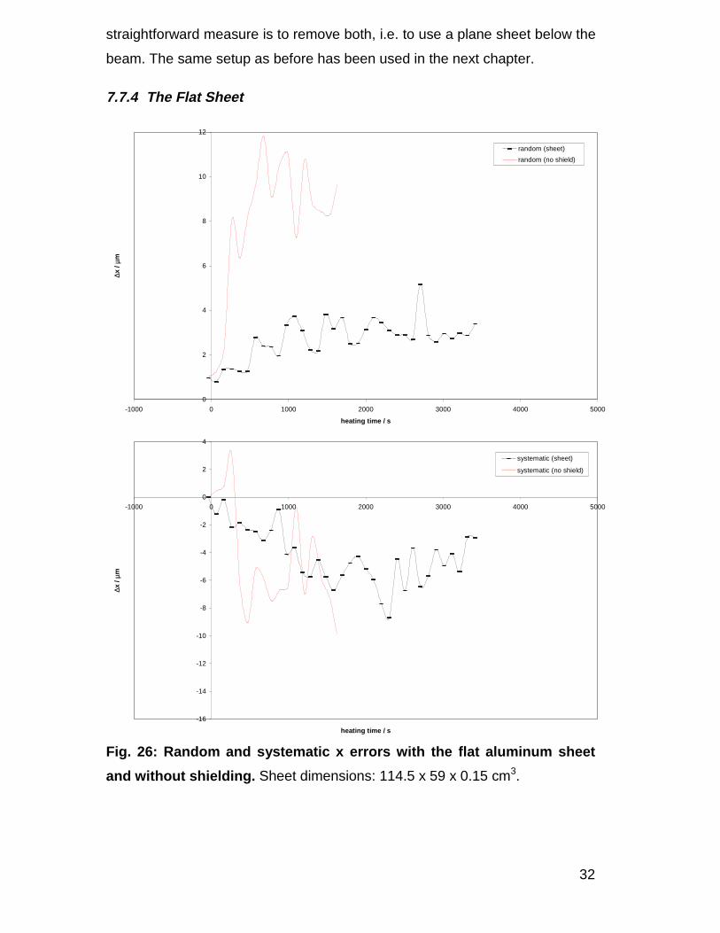
7.7.4 The Flat Sheet
0
2
4
6
8
10
12
-1000 0 1000 2000 3000 4000 5000
heating time / s
∆x /
µm
random (sheet)
random (no shield)
-16
-14
-12
-10
-8
-6
-4
-2
0
2
4
-1000 0 1000 2000 3000 4000 5000
heating time / s
∆x /
µm
systematic (sheet)
systematic (no shield)
Fig. 26: Random and systematic x errors with the flat aluminum sheet
and without shielding. Sheet dimensions: 114.5 x 59 x 0.15 cm3.

33
0
2
4
6
8
10
12
14
-1000 0 1000 2000 3000 4000 5000
heating time / s
∆y /
µm
random (sheet)
random (no shield)
-13
-11
-9
-7
-5
-3
-1
1
3
5
-1000 0 1000 2000 3000 4000 5000
heating time / s
∆y /
µm
systematic (sheet)
systematic (no shield)
Fig. 27: Random and systematic y errors with the flat aluminum sheet
and without shielding.
34
0.0000
0.0001
0.0002
0.0003
0.0004
0.0005
0.0006
0.0007
0.0008
0.0009
0.0010
-500 0 500 1000 1500 2000 2500 3000 3500 4000 4500 5000
heating time / s
∆M /
M0
random (sheet)
random (no shield)
-0.0005
-0.0003
-0.0001
0.0001
0.0003
0.0005
0.0007
0.0009
0.0011
-500 0 500 1000 1500 2000 2500 3000 3500 4000 4500 5000
heating time / s
M /
M0 -
1
systematic (sheet)
systematic (no shield)
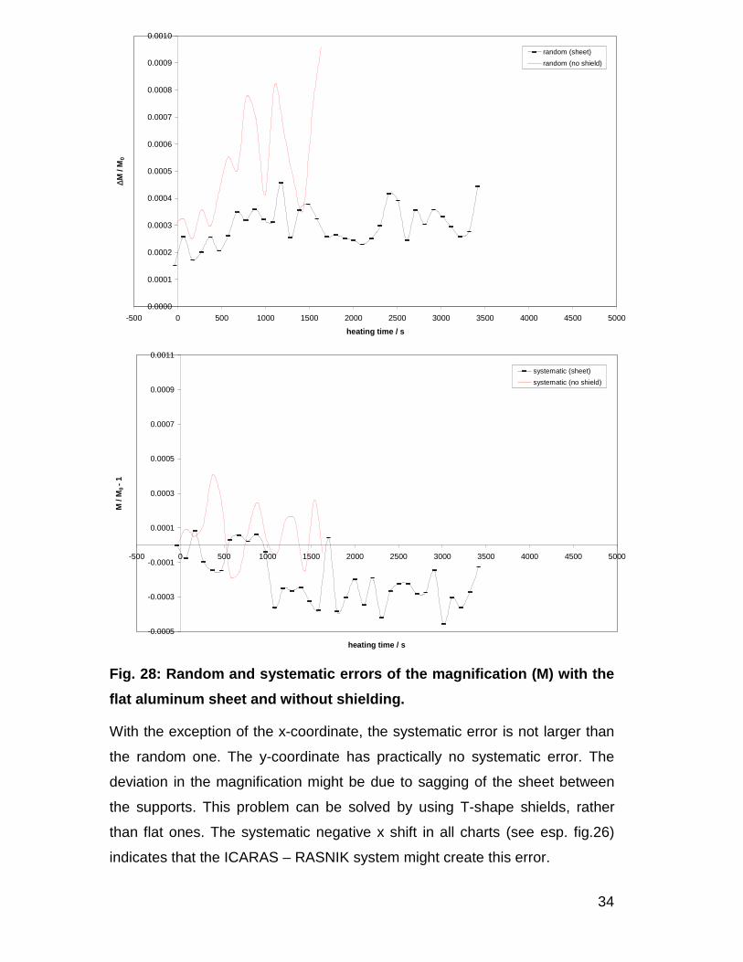
Fig. 28: Random and systematic errors of the magnification (M) with the
flat aluminum sheet and without shielding.
With the exception of the x-coordinate, the systematic error is not larger than
the random one. The y-coordinate has practically no systematic error. The
deviation in the magnification might be due to sagging of the sheet between
the supports. This problem can be solved by using T-shape shields, rather
than flat ones. The systematic negative x shift in all charts (see esp. fig.26)
indicates that the ICARAS – RASNIK system might create this error.

35
8. ERROR ANALYSIS
If errors of measurement values are relatively small compared to others, they
will be neglected in the following equations.
Equation 5:∞
∞∆=∆
M
M
pp
Equation 7:erceptinterceptint
cc ∆=∆
Equation 16:tb
tb
tt
)tt(
hh
KK
−−∆
+∆=∆
Equation 25:l)ab(2
l)ab(2KK
y)y(
−−∆+∆+∆+∆=
∆∆∆
Equation 28:fg
gl)ag(2
l)ag(2KK
y)y(
−∆+
−−∆+∆+∆+∆=
∆∆∆
Equation 29: t)t1(
nn
20 ∆α+
α∆=∆
9. CONCLUSION
With the method given the effective pixel size was determined with a relative
accuracy of 4.7.10-5 and the distance between ccd diode array and protection
glass with a relative accuracy of 7.4 %. No significant mask pitch variations
(smaller than 0.3 microns over 20 mm) of the 120 microns mask were
measured. However, ccd pitch variations of up to 2.10-3 were observed. The
ultimate performance revealed an rms of 0.1 µm in the x- and y-coordinates,
and a relative random error in the magnification of 3.10-5. Linearity could be
shown for the x-, y-, z-, and rot z – coordinates. The values of rot x and rot y
could be used as qualitative indicators of rotational movements at best. The
minimum required LED current for illuminating the mask was indicated by a
failure of the ICARAS system rather than a rise of the random error.
Theoretical and measured image displacements caused by a constant air
temperature gradient agreed within the error tolerance. The systematic errors
created by common shields in a heat dissipating environment gave rise to
using plane metal sheets which proved better.

36
10. FILES INDEX
All data used for plots and tables are stored as files on “Heinz” in the directory
c:\Gary. In order to get the original ICARAS files which are stored in the
directory c:\Results\Tempresults, one has to add the number “19” before the
Excel file name and change the extension into “res”. This rule is only valid for
files with date names.
Chapter 3: 970526.xls
970716.xls
970717.xls
Tab.1: 970516.xls
Tab.2: Report.xls
970707.xls
970708.xls
Fig.4: 970612.xls
Fig.5: 970612.xls
Fig.6: 970611.xls
Fig.7: 970618.xls
Fig.8: 970618.xls
Fig.9: 970618.xls
Fig.10: 970613.xls
Fig.14: 970630.xls
Fig.15: 970624.xls
Fig.16: 970701.xls
Fig.17: 970714ns.xls
Fig.18: 970709.xls
Fig.19: 970709.xls
Fig.20: shielding.xls
970711.xls
970714.xls
Fig.21: shielding.xls
970709.xls
970710.xls
Fig.22: shielding.xls
970711.xls
970714.xls
Fig.23: shielding.xls
970709.xls
970710.xls
Fig.24: shielding.xls
970711.xls
970714.xls
Fig.25: shielding.xls
970709.xls
970710.xls
Fig.26: shielding.xls
970714.xls
970714ns.xls
Fig.27: shielding.xls
970714.xls
970714ns.xls
Fig.28: shielding.xls
970714.xls
970714ns.xls