system simulation of mechatronic clutch in automatic transmission
TRANSCRIPT
System Simulation of Mechatronic Clutch in Automatic Transmission Drivelines
Master’s Thesis in the Systems, Control and Mechatronics
MUDDASSAR PIRACHA, UMER SOHAIL Department of Applied Mechanics Division of Dynamics CHALMERS UNIVERSITY OF TECHNOLOGY Göteborg, Sweden 2011 Master’s Thesis 2011:15

I
MASTER’S THESIS 2011:15
System Simulation of Mechatronic Clutch in Automatic Transmission Drivelines
MASTER’S THESIS IN THE SYSTEMS, CONTROL AND MECHATRONICS
MUDDASSAR PIRACHA, UMER SOHAIL
Department of Applied Mechanics Division of Dynamics
CHALMERS UNIVERSITY OF TECHNOLOGY
Göteborg, Sweden 2011

II
System Simulation of Mechatronic Clutch in Automatic Transmission Drivelines Master’s Thesis in the Systems, Control and Mechatronics MUDDASSAR PIRACHA, UMER SOHAIL
© Muddassar Piracha, Umer Sohail, 2011
Master’s Thesis 2011:15 ISSN 1652-8557 Department of Applied Mechanics Division of Dynamics Chalmers University of Technology SE-412 96 Göteborg Sweden Telephone: + 46 (0)31-772 1000 Cover: Fig 5 The Torque converter as a system, LUK Colloquium, Page 129, (modified) Printed: Chalmers Reproservice Göteborg, Sweden 2011
III
System simulation of Mechatronic Clutch in Automatic Transmission Drivelines Master’s Thesis in Systems, Control and Mechatronics MUDDASSAR PIRACHA, UMER SOHAIL Department of Applied Mechanics Division of Dynamics Chalmers University of Technology
ABSTRACT
In this master thesis project, an automatic transmission vehicular driveline model has been further developed in AMESim modeling environment. The main work has been put in the development of mechatronic clutch system which is a combination of dynamic torque converter, torque converter clutch (TCC) damper and lock-up clutch. Previously, TCC damper and lock-up clutch were already present in the system but having conflict with the real system. The whole system is then rebuilt again according to conventional torque converter layout.
A nonlinear model of hydro-dynamic torque converter has been introduced which takes into account the transient behavior of the fluid for even high frequency range of velocities.
The simulation model is then used to optimize the fuel consumption and NVH (noise, vibration, harshness) behavior of the system at a particular range of velocities. The multi-objective and conflicting optimization problem is solved by using advanced solving algorithms such as genetic algorithm. The algorithm gives best solution at a particular velocity instance.
The solution is provided in the form of a look-up table containing slip values at particular velocities for best NVH and fuel consumption. The look-up table is then embedded into the controller and the strategy known as ECCC (electronically controlled converter clutch) slip control strategy is developed.
Key words:
Dynamic torque converter, ECCC slip control strategy, Fuel consumption, Pareto optimization, NVH

IV

CHALMERS, Applied Mechanics, Master’s Thesis 2011:15 V
Contents 1 INTRODUCTION ...................................................................................................................... 1
1.1 BACKGROUND ................................................................................................................................ 1 1.2 PROBLEM STATEMENT ..................................................................................................................... 1 1.3 DRIVELINE THEORY .......................................................................................................................... 2
1.3.1 Basic Driveline Equations .................................................................................................. 3 1.3.1.1 Engine ................................................................................................................................... 3 1.3.1.2 Clutch .................................................................................................................................... 3 1.3.1.3 Transmission ......................................................................................................................... 3 1.3.1.4 Drive Shaft/Side Shaft ........................................................................................................... 3 1.3.1.5 Wheels .................................................................................................................................. 4 1.3.1.6 Flexible Clutch ....................................................................................................................... 5 1.3.1.7 Nonlinear Clutch ................................................................................................................... 5 1.3.1.8 Flexible Driveshaft ................................................................................................................. 6 1.3.1.9 Planetary Gear Set Transmission .......................................................................................... 6 4th Gear ..................................................................................................................................................... 9 5th Gear ...................................................................................................................................................... 9
1.4 MECHATRONIC CLUTCH SYSTEM ...................................................................................................... 10 1.4.1 Torque Converter ............................................................................................................ 11
1.4.1.1 Working Principle ................................................................................................................ 12 1.4.1.2 Modeling ............................................................................................................................. 13
1.4.2 Lock‐up Clutch and TCC Damper ..................................................................................... 16
2 COMPUTATIONAL MODEL .................................................................................................... 17
2.1 CURRENT MODEL .......................................................................................................................... 17 2.1.1 Engine ............................................................................................................................. 17
2.1.1.1 Torque Generation .............................................................................................................. 17 2.1.1.2 Oscillating Force generation ............................................................................................... 19
2.1.2 Torque Converter Damper .............................................................................................. 19 2.1.3 Transmission (AF‐40) ...................................................................................................... 22 2.1.4 Side Shafts ....................................................................................................................... 26 2.1.5 Mechatronic Clutch ......................................................................................................... 26
3 VERIFICATION ....................................................................................................................... 28
3.1 TORQUE CONVERTER ...................................................................................................................... 28 3.2 MECHATRONIC CLUTCH .................................................................................................................. 32
3.2.1 Lock‐up clutch fully disengaged ...................................................................................... 33 3.2.2 Lock‐up clutch partially engaged .................................................................................... 35 3.2.3 Lock‐up clutch fully engaged .......................................................................................... 39
4 VALIDATION ......................................................................................................................... 42
5 ECCC SLIP CONTROL STRATEGY ............................................................................................. 50
5.1 WORKING PRINCIPLE OF SLIP CONTROLLER .......................................................................................... 50 5.1.1 Control loop .................................................................................................................... 51 5.1.2 Output characteristics of controller ................................................................................ 51
6 OPTIMIZATION ..................................................................................................................... 54
6.1 FUEL CONSUMPTION ..................................................................................................................... 54 6.2 NVH CHARACTERISTICS .................................................................................................................. 55 6.3 CONFLICTING CRITERION ................................................................................................................ 55 6.4 OPTIMIZATION APPROACH .............................................................................................................. 56
6.4.1 AMESim model ................................................................................................................ 56 6.4.2 Simulink model ................................................................................................................ 57 6.4.3 Fitness Function .............................................................................................................. 57 6.4.4 Optimization Toolbox ...................................................................................................... 58
6.5 RESULTS FROM OPTIMIZATION ......................................................................................................... 59

CHALMERS, Applied Mechanics, Master’s Thesis 2011:15 VI
6.6 DISCUSSION ON RESULTS ................................................................................................................. 62 6.7 DEVELOPMENT OF LOOK UP TABLE FOR ECCC SLIP CONTROL .................................................................. 63 6.8 SENSITIVITY ANALYSIS OF END‐STOP ANGLES OF TCC DAMPER ................................................................ 64
7 CONCLUSION ........................................................................................................................ 68
8 FUTURE WORK ..................................................................................................................... 69
9 REFERENCES ......................................................................................................................... 70
CHALMERS, Applied Mechanics, Master’s Thesis 2011:15 VII
Preface
This master thesis is the final part of our master education in Systems, Control and Mechatronics at the Chalmers University of Technology. The work has been carried out at the division of Dynamics, Department of Applied Mechanics at CHALMERS with close coordination with SAAB Automobile Powertrain AB and VICURA AB, located in Trollhättan. First of all we would like to thank our examiner and supervisor, Professor Viktor Berbyuk, for his guidance and help in this thesis. Furthermore, we would like to thank our supervisors from SAAB, Sohail Iftikhar, Michael Svensson and Engineering Manager Per Rosander. We would also like to thank Torbjörn Kvist, Mikael Sjöstrand, Martin Johansson and Christoffer Ståhl from VICURA AB for their support, help and hints. The thesis work can be divided into three distinctive parts: modeling, verification and validation, and optimization. In the modeling part, torque converter model is developed by Muddassar while Umer has done the modeling of transmission and rest of the Mechatronic clutch. Verification and validation is done by Umer while Muddassar has developed the optimization routine. Muddassar Piracha, Umer Sohail Göteborg, June 2011.
CHALMERS, Applied Mechanics, Master’s Thesis 2011:15 VIII
Notations
, Net flow areas perpendicular to at impeller and stator exits (Assumption 1: )
= Maximum vehicle cross section area
= Drag coefficient
, , , , , Shock loss coefficients (Ideally equal to 1), determined experimentally in practice
System kinetic co-energy
F = Clutch dynamic torque
= Clutch frictional torque
0.2 0.3, Fluid friction factors
= Friction force
= Rolling Resistance
= Air drag force
= Gravitational force
, , Unit vectors corresponding to polar coordinates in the radial direction, the tangential direction, and the direction along the torque converter axis
, Impeller fluid polar moment of inertia
, Impeller mechanical polar moment of inertia
= Conversion ratio of gears
= Mass moment of inertia of the engine
Total length of the axial projection of meridianal line contained within impeller
= Mass of the vehicle
Net input power,
System power loss due to flow and fluid shock losses
Spatially constant
, Mean radii at impeller and stator exits
Radius leading to fluid particle at or
= Clutch torque
= Transmission output/ Driveshaft input torque
= Driving torque
_ Engine output torque
, = Internal frictional torque from engine

CHALMERS, Applied Mechanics, Master’s Thesis 2011:15 IX
_ _ Side shaft input torque
= Clutch output/Transmission input torque
= Wheel torque
Axial torus flow velocity with spatially constant magnitude
V = Relative velocity between two clutch surfaces
, , , , , Shock velocities
= Slope of the road
Blade angle with respect to plane A
= Clutch angular displacement
= Crankshaft angle
, Blade angles with respect to impeller and stator exits
= Transmission angular displacement
= Wheels angular displacement
= Clutch angular speed
2 , Engine speed
= Transmission angular speed
= Wheels rotational speed
, , Blade angles with respect to plane A at impeller, turbine and stator entrances respectively
Fluid mass density
= Air density
Impeller torque,
tan , Fluid velocity relative to blades
Absolute fluid velocity; , ,
= Acceleration of vehicle
Engine output velocity
, Impeller, stator speed
= Impeller rotary velocity
Side shaft input velocity
= Turbine rotary velocity
_ Angular acceleration of engine at present time t
_ Max acceleration defined for acceptable NVH characteristic
_ _ Angular acceleration of side shaft at present time t

CHALMERS, Applied Mechanics, Master’s Thesis 2011:15 X
Total fluid volume equal to the sum of the three control volumes

CHALMERS, Applied Mechanics, Master’s Thesis 2011:15 1
1 Introduction
1.1 Background
Previously, a driveline model of an automatic transmission car has been created in AMESim (Simulation software for modeling and analysis of one dimensional system). The model contains sub-models of engine, Torque converter damper, power-train mounts, transmission, differentials, drive shafts and wheels. The entire model simulates speed and torque signals from different parts of the driveline and NVH characteristics are studied from acceleration signals.
In the automotive industry today, more and more of the development is driven by virtualization. Due to the fact that the development cycles are becoming shorter and has to be more cost efficient, less hardware is available for performing actual tests in vehicles and in test benches. Furthermore, the integration process of existent and newly developed components into a complete driveline is a delicate task and usually requires lots of tests to secure the design. Whereas in the past, it was enough to simulate each subsystems separately, some of them were simulated and tested on hardware. But due to recent advancements in the computational power, more complex and realistic simulation softwares are being used for simulation of complex physical systems composed of subsystems from different areas, such as mechanical, electrical, hydraulic and control systems collectively. The simulations are typically used to optimize products and to reduce costs and time in the product development process.[19]
It is much more economical and time efficient to design and test the products by computer simulations before building their prototypes. Also, the performance can be predicted easily and closely. Moreover, Simulations can be helpful for tunning parameters and setting to improve the subsystems and ultimately resulting in higher quality of the final product. Simulations also increase the opportunities to test different functions and versions by very simple changes. Also, powerful optimization algorithms have made it possible to optimize the performance of different components by using algorithm softwares.
Nowadays, efforts are being put to improve the fuel efficiency of an automatic transmission car. The torque converter is a very good launching device for automatic transmissions but is inefficient in steady state modes because the fluid coupling in the torque converter does not allow the whole torque to transmit which reduces the fuel efficiency. Although, reducing the slip of torque converter minimizes the losses due to fluid coupling, but it also reduces the damping provided by the slipping torque and as a result the sensitivity of driveline to engine excitations increases.[13]
1.2 Problem Statement
The purpose of this project is to further develop and optimize NVH system model library for complete vehicle drivelines. The development phase involves introducing dynamic torque converter and lockup clutch along with already developed torque
CHALMERS, Applied Mechanics, Master’s Thesis 2011:15 2
converter damper. A further goal is to establish an ECCC slip control strategy for applying an optimal tradeoff between fuel economy and driving comfort. Optimization algorithm will be used to find an optimal path which will ensure minimum fuel consumption as well as minimum NVH characteristics.
The main focus of the project will be on following folds:
Develop the mathematical and computational model of complete torque converter known as Mechatronic clutch and embed in current driveline model in AMESim. Verify and validate the model.
Optimize the driveline model in order to find an optimal tradeoff between fuel consumption and NVH characteristics.
Develop an ECCC slip control strategy to achieve optimized driveline model.
The first chapter deals with basic definitions of vehicular driveline. Second chapter explains the current driveline model along with further developments. Third and fourth chapters include verification and virtual validation of further developed computational model. Chapter five explains the slip controller and chapter six describes optimization which results in ECCC slip control strategy and also sensitivity analysis of some physical parameters of TCC damper.
1.3 Driveline Theory
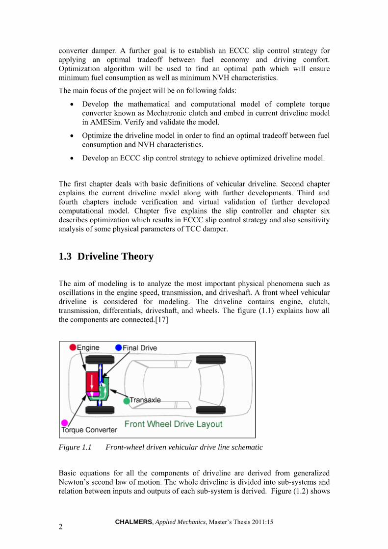
The aim of modeling is to analyze the most important physical phenomena such as oscillations in the engine speed, transmission, and driveshaft. A front wheel vehicular driveline is considered for modeling. The driveline contains engine, clutch, transmission, differentials, driveshaft, and wheels. The figure (1.1) explains how all the components are connected.[17]
Figure 1.1 Front-wheel driven vehicular drive line schematic
Basic equations for all the components of driveline are derived from generalized Newton’s second law of motion. The whole driveline is divided into sub-systems and relation between inputs and outputs of each sub-system is derived. Figure (1.2) shows

CHALMERS, Applied Mechanics, Master’s Thesis 2011:15 3
labels, inputs, and outputs of each sub-system in the driveline as explained by Kiencke and Nielsen. [10]
Figure 1.2 Sub-systems of a vehicular driveline
1.3.1 Basic Driveline Equations
1.3.1.1 Engine
The output torque of the engine is obtained by driving torque ( ) resulting from combustion, the internal friction from the engine ( , ), and the external load from the clutch ( ). Applying Newton’s second law, we get:
, 1.1
1.3.1.2 Clutch
A friction clutch consists of a clutch disk connecting the flywheel of the engine and the transmission’s input shaft. The clutch is assumed to be stiff. When the clutch is engaged with assumption of no internal friction, we obtain . The transmitted torque is a function of angular difference and angular velocity difference over the clutch
, 1.2
1.3.1.3 Transmission
A transmission has a set of gears, each with a conversion ratio . We get the following relation between input and output torque of the transmission:
, , , , , 1.3
1.3.1.4 Drive Shaft/Side Shaft
The drive shafts connect the wheels with the transmission. They are assumed to be stiff. It is also assumed that both the wheels have same rotational speed . The

CHALMERS, Applied Mechanics, Master’s Thesis 2011:15 4
vehicle dynamics are neglected; the rotational equivalent wheel speed shall be equal to the vehicle body’s centre of gravity.
1.4
Hence, drive shafts are modeled as one shaft. When the vehicle is turning, then both the drive shafts have to be modeled. Neglecting friction , gives the model equation:
, 1.5
1.3.1.5 Wheels
Newton’s second law in the longitudinal direction gives the following equation:
sin 1.6
Figure 1.3 Longitudinal Forces acting on a vehicle
The air drag is approximated by:
12
1.7
The rolling resistance is approximated by:
1.8
, depend on tires and tire pressure
The resultant torque due to , where is the wheel radius. Newton’s second law gives:
1.9
CHALMERS, Applied Mechanics, Master’s Thesis 2011:15 5
The dynamic influence from the tire has been neglected. Including (1.6) to (1.8) in (1.9) together with gives
12sin 1.10
Some components in the driveline need to have modified models in order to ensure the correct behavior in simulation environment. However, the complexity of the system will increase. The components are clutch, transmission, and drive shaft.
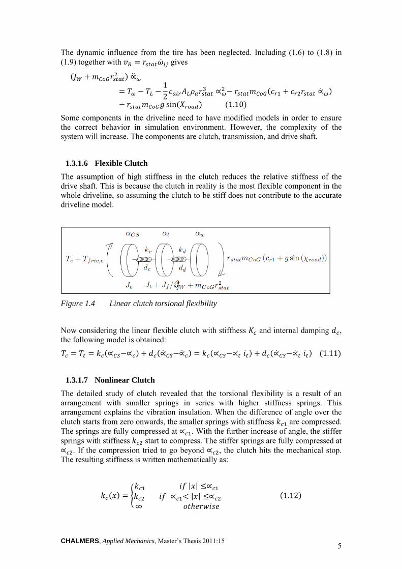
1.3.1.6 Flexible Clutch
The assumption of high stiffness in the clutch reduces the relative stiffness of the drive shaft. This is because the clutch in reality is the most flexible component in the whole driveline, so assuming the clutch to be stiff does not contribute to the accurate driveline model.
Figure 1.4 Linear clutch torsional flexibility
Now considering the linear flexible clutch with stiffness and internal damping , the following model is obtained:
1.11
1.3.1.7 Nonlinear Clutch
The detailed study of clutch revealed that the torsional flexibility is a result of an arrangement with smaller springs in series with higher stiffness springs. This arrangement explains the vibration insulation. When the difference of angle over the clutch starts from zero onwards, the smaller springs with stiffness are compressed. The springs are fully compressed at . With the further increase of angle, the stiffer springs with stiffness start to compress. The stiffer springs are fully compressed at
. If the compression tried to go beyond , the clutch hits the mechanical stop. The resulting stiffness is written mathematically as:
| | | |
∞ 1.12

CHALMERS, Applied Mechanics, Master’s Thesis 2011:15 6
The torque from the clutch nonlinearity is
| | | |
∞
1.13
The nonlinear phenomenon of clutch is explained in the figure (1.5) below.
Figure 1.5 Nonlinear clutch characteristics
The nonlinear characteristic of the clutch makes it a very good damper and is very useful for damping out torsional vibrations propagating from engine. Automatic transmission vehicles have replaced the mechanical clutch with a mechatronic clutch, which is a system of dynamic torque converter, lock-up clutch and damper. The characteristics of lock-up clutch with damper are the same as explained in the section of nonlinear clutch. The dynamic torque converter is briefly explained in the next section.
1.3.1.8 Flexible Driveshaft
By modeling the drive shaft as a damped torsional flexibility of stiffness , internal damping , the equation (1.5) becomes
1.5
1.3.1.9 Planetary Gear Set Transmission
Automatic transmission contains many gears in various combinations. The gears are never physically moved and are always engaged to the same gears with different combinations. This is achieved by using a special kind of gear set called planetary gear sets as shown in the figure (1.6). While in manual transmission, when the shift
CHALMERS, Applied Mechanics, Master’s Thesis 2011:15 7
lever is moved from one position to another position, gears slide along the shafts to engage various sized gears to acquire correct gear ratio.
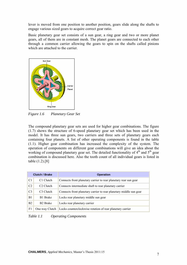
Basic planetary gear set consists of a sun gear, a ring gear and two or more planet gears, all of them are in constant mesh. The planet gears are connected to each other through a common carrier allowing the gears to spin on the shafts called pinions which are attached to the carrier.
Figure 1.6 Planetary Gear Set
The compound planetary gear sets are used for higher gear combinations. The figure (1.7) shows the structure of 6-speed planetary gear set which has been used in the model. It has three sun gears, two carriers and three sets of planetary gears each containing four planets. A list of other operating components is found in the table (1.1). Higher gear combination has increased the complexity of the system. The operation of components on different gear combinations will give an idea about the working of compound planetary gear set. The detailed functionality of 4th and 5th gear combination is discussed here. Also the tooth count of all individual gears is listed in table (1.2).[8]
Clutch / Brake Operation
C1 C1 Clutch Connects front planetary carrier to rear planetary rear sun gear
C2 C2 Clutch Connects intermediate shaft to rear planetary carrier
C3 C3 Clutch Connects front planetary carrier to rear planetary middle sun gear
B1 B1 Brake Locks rear planetary middle sun gear
B2 B2 Brake Locks rear planetary carrier
F1 One-way Clutch Locks counterclockwise rotation of rear planetary carrier
Table 1.1 Operating Components

CHALMERS, Applied Mechanics, Master’s Thesis 2011:15 8
Figure 1.7 Compound Planetary Gear Set
Gears No. of Teeth
S1 Sun Gear 45
R1 Ring Gear 81
P1 Pinion/Planet Gear 17
S2 Sun Gear 33
R2 Ring Gear 72
P2 Pinion/Planet Gear 18
S3 Sun Gear 27
R3Ring Gear = R2 ring gear 72
P3.1 Pinion/Planet Gear 18
P3.2 Pinion/Planet Gear 17
Counter – Drive 53
Counter – Driven 48
Final gear - Drive 15
Final gear - Driven 53
Table 1.2 Tooth count AF-40 transmission
CHALMERS, Applied Mechanics, Master’s Thesis 2011:15 9
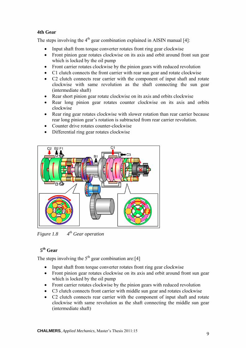
4th Gear
The steps involving the 4th gear combination explained in AISIN manual [4]:
Input shaft from torque converter rotates front ring gear clockwise Front pinion gear rotates clockwise on its axis and orbit around front sun gear
which is locked by the oil pump Front carrier rotates clockwise by the pinion gears with reduced revolution C1 clutch connects the front carrier with rear sun gear and rotate clockwise C2 clutch connects rear carrier with the component of input shaft and rotate
clockwise with same revolution as the shaft connecting the sun gear (intermediate shaft)
Rear short pinion gear rotate clockwise on its axis and orbits clockwise Rear long pinion gear rotates counter clockwise on its axis and orbits
clockwise Rear ring gear rotates clockwise with slower rotation than rear carrier because
rear long pinion gear’s rotation is subtracted from rear carrier revolution. Counter drive rotates counter-clockwise Differential ring gear rotates clockwise
Figure 1.8 4th Gear operation
5th Gear
The steps involving the 5th gear combination are:[4]
Input shaft from torque converter rotates front ring gear clockwise Front pinion gear rotates clockwise on its axis and orbit around front sun gear
which is locked by the oil pump Front carrier rotates clockwise by the pinion gears with reduced revolution C3 clutch connects front carrier with middle sun gear and rotates clockwise C2 clutch connects rear carrier with the component of input shaft and rotate
clockwise with same revolution as the shaft connecting the middle sun gear (intermediate shaft)

CHALMERS, Applied Mechanics, Master’s Thesis 2011:15 10
Rear long pinion gear rotates clockwise on its axis and orbits clockwise. The rear short pinion gear is pushed out by the speed difference because the rear carrier rotates faster than the middle sun gear and orbits clockwise while rotating clockwise on its axis.
Rear ring gear rotates clockwise with faster revolution than rear carrier because rear long pinion gear’s rotation is added to the rear carrier’s revolution.
Counter drive rotates counter-clockwise Differential ring gear rotates clockwise
Figure 1.9 5th Gear operation
1.4 Mechatronic Clutch System
In automatic transmission, the clutch is replaced by Mechatronic clutch system, a combination of three components; Torque Converter, Lock-up Clutch, and TCC (Torque Converter Clutch) Damper. The control strategy determines the requirements for different operating ranges. The figure (1.10) shows the Mechatronic clutch system between engine and transmission.[5]
Figure 1.10 Mechatronic Clutch System

CHALMERS, Applied Mechanics, Master’s Thesis 2011:15 11
The physical placement of all the components is shown in figure (1.11) presented by Paul.[13] It is clearly seen that the torque converter is in parallel with lock-up clutch and TCC damper, while lock-up clutch and TCC damper are connected in series. Engine is the input to the Mechatronic clutch system which is connected to the transmission at output. The engine torque can be transmitted entirely via torque converter or the lock-up clutch and TCC damper or both, depending on whether the lock-up clutch is fully disengaged, fully engaged or partially engaged. The components are explained in detail in the coming sections.
1.4.1 Torque Converter
Torque converter is a hydrodynamic coupling element between engine and automatic transmission. This coupling element is advantageous over traditional manual transmission mechanical coupling because of the principle of hydrodynamic power transfer from engine to transmission. Its application in the driveline has improved performance and acceleration. Its main benefit is the increased isolation of engine torsional vibrations due to the slip which provides comfortable transmission shifts. [2]
Figure 1.11 TCC Damper Placement in a Mechatronic Clutch System
Torque converter was first introduced in 1940s. At that time, the main focus was on increasing the driver’s comfort. The performance and fuel economy factors were not important. The functionality and complexity was also very high as compared to those used today. Nowadays, fuel economy and performance are very important factors along with the comfort. [5]
Torque converter is a very critical element that affects fuel economy, vehicle performance, and drive quality. Keeping that in view, an accurate model of torque converter is needed. This model will be helpful to investigate the dynamics of fast

CHALMERS, Applied Mechanics, Master’s Thesis 2011:15 12
transients that occur during fast speed ratio changes, the influence of torque pulses on power train dynamics and possibly the torque converter design changes.
1.4.1.1 Working Principle
A torque converter has three main parts i.e. impeller which is attached to the engine, turbine which is splined to the input shaft of transmission, and the stator which is attached to the transmission housing through one-way clutch as shown in the figure (1.12). All three components have canted blades similar to that of a fan as shown in the figure (1.13). The converter assembly is filled with transmission fluid. The arrows in the figure (1.13) show the direction of motion of transmission fluid. [6]
As the engine spins the impeller, the blades of impeller pick up the fluid and force it towards the turbine with some pressure. If the resistance of drive train is greater than the force of fluid, the turbine remains still and so as the vehicle. [11]
Figure 1.12 Torque converter Assembly
At lower speeds; when turbine has lower spinning than impeller, the fluid leaves the turbine with an angle and enters into the stator. The blades of the stator redirect the fluid towards the impeller with increased pressure, where its pressure is increased again by the impeller towards the turbine. This phenomenon is called torque multiplication. That’s why automatic transmission vehicles have greater torque than manual transmission vehicles at lower speeds. One way roller clutch prevents the stator from spinning backwards which would affect torque multiplication.
When the turbine picks up the speed, the fluid is sent outwards due to the centrifugal effect and prevented from going back towards the impeller. When turbine is running at 90% of the impeller speed, the fluid starts to hit at the back of stator blades, the roller clutch is unlocked and the stator is forced to rotate in the direction of impeller and turbine. This phenomenon is called coupling phase.
At vehicle launching phase, the impeller is rotating and turbine isn’t, the difference in speed creates vortex flow which causes the full torque multiplication which causes

CHALMERS, Applied Mechanics, Master’s Thesis 2011:15 13
tremendous heat loss and reduces the efficiency. As the engine picks up the speed, the coupling phase occurs and reduces vortex flow which increases the efficiency and reduces heat loss.
The conventional torque converter never achieves 100% coupling because the fluid is being used as power transfer causing some of the torque to dissipate as heat which creates slip. Thus, the high speed efficiency of automatic transmission vehicle is suffered. This problem is solved by the introduction of lock-up clutch in the torque converter operated by solenoid valve. This clutch is usually engaged at steady state speed to enhance fuel efficiency. Nowadays, friction plate lock-up clutch is being introduced to effectively control the slip and to further improve fuel efficiency. [5]
Figure 1.13 Torque converter Components
1.4.1.2 Modeling
The torque converter model is developed based on following assumptions: [16]
The cross-sectional net torus flow area is constant around the torque converter flow path which implies constant axial torus flow velocity.
The actual flow is approximated by streamline flow or laminar flow.
The spacing between torque converter parts is neglected.
The blade thickness effects are neglected.
Thermal effects are not considered.
During torque multiplication phase, the torque converter dynamics are represented by four first-order nonlinear differential equations in four state variables which correspond to fluid, impeller, stator and turbine inertias.
The equations for impeller, stator and turbine inertias follow from the application of moment-of-momentum equation while the equation for fluid inertia is obtained from the power balance for the torque converter system. During torque multiplication phase, only three equations will be valid because the stator is stationary by the action of one-way clutch.

CHALMERS, Applied Mechanics, Master’s Thesis 2011:15 14
Figure 1.14 Side view schematic of a torque converter
Figure 1.15 Fluid enter and exit angles across turbine, impeller and stator
The dynamical principle can be expressed in a quite simple and compact way as shown in [3]
1
Where
is the state vector,
, 2
: the input vector,

CHALMERS, Applied Mechanics, Master’s Thesis 2011:15 15
0 0 3
: the loss vector,
0 0 0 4
The shock and friction loss is given by:
2 5
0.2 0.3, Fluid friction factors
is the inertia matrix,
0 0
0
0 0
0 6
: 4 4 is the multiport, modulated gyrator matrix function,
0 7
0 00 00 0
8
vector value when 0
. . tan . . tan
. . tan . . . tan
. . tan . . . tan
9
vector value when 0
. . tan . . . tan
. . tan . . tan
. . tan . . tan
10

CHALMERS, Applied Mechanics, Master’s Thesis 2011:15 16
1.4.2 Lock-up Clutch and TCC Damper
The lock-up clutch is installed on the turbine hub between the turbine and the converter front cover. The stick slip behavior of lock-up clutch is explained by Singh. [14]. Hydraulic pressure on either side of the converter piston causes it to engage or disengage the converter front cover. A set of damping springs called TCC damper absorb the torsional force upon clutch engagement to prevent shock transfer. The figure (1.16) shows the placement of lock-up clutch and TCC damper. The difference of fluid pressure on either side of the lock-up clutch determines the engagement or disengagement. Fluid can either enter the body of the converter behind the lock-up clutch for engagement, or in front of the lock-up clutch for disengagement. The power flow is color coded; Green: input power, Blue: output power. It is interesting to see that no torque goes through the impeller in ‘lock-up on’ mode while turbine is being used. [15]
Figure 1.16 Lock-up off
Figure 1.17 Lock-up on

CHALMERS, Applied Mechanics, Master’s Thesis 2011:15 17
2 Computational Model
2.1 Current Model The block diagram of SAAB’s current model is given in the figure (2.1) below:
Figure 2.1 Current Model Layout
As the emphasis of the thesis is on driveline therefore the detailed description of torque converter damper, transmission and side shafts will be given. The functional description of engine is also provided.
2.1.1 Engine
The computational model in AMESim is shown in figure (2.2). The engine can be divided in two parts for better understanding.
2.1.1.1 Torque Generation
The first part as shown by figure (2.3) is responsible for the torque generation. The basic principle of the torque generation is as follows.
The engine starts rotating at the beginning of the simulation by a Global variable defined as IC_rev, which is engines initial velocity and is set to 1000 rpm. The torque generated from the engine revolving at this velocity is calculated by piecewise linear function (indicated by blue box in the figure) between average velocity and torque at wide open throttle. The torque generated is called the average torque (signal path is shown by yellow line in figure). The torque spikes generated due to combustion are calculated by the empirical formulas. These empirical formulas are based on the physical characteristics of the engine (there implementation is represented by the constituents of the black box).
Engine Torque converter
damper
Transmission
Side Shafts Wheels
Power Train Mounts

CHALMERS, Applied Mechanics, Master’s Thesis 2011:15 18
Figure 2.2 Torque Converter with Lock-up Clutch and TCC Damper
Finally the sum of the average torque and torque spikes is added (at the summer indicated by blue circle) and the sum (represented by grey line) is applied on the ‘’Engine and Primary side inertia’’. The torque and angular velocity of this inertia is the output from engine to the torque converter damper.
Figure 2.3 Torque Generation from engine

CHALMERS, Applied Mechanics, Master’s Thesis 2011:15 19
2.1.1.2 Oscillating Force generation
The angle and angular velocity of the output shaft of the engine are fed to the empirical formulas implemented inside the dotted blue line and the output is fed to the power train mounts as shown in the figure (2.4).
Figure 2.4 Oscillating force generation from engine.
2.1.2 Torque Converter Damper
The computational model of torque converter damper is implemented as shown in the figure (2.5). The input to the damper is torque and angular velocity from the engine and at its output transmission is connected. Another input to the damper is the mean rpm of the engine which commands the friction in the clutch.
Figure 2.5 Computational model of TCC Damper

CHALMERS, Applied Mechanics, Master’s Thesis 2011:15 20
The computational model with all the labels of the components used is shown in the figure (2.6).
Figure 2.6 Detailed computational model of Torque Converter Damper
The input from the engine after passing through angle sensor ADT00-6 enters the port 3 of the link TRLI0C-2. The causality and port numbers of this component is shown in the figure (2.7).
Figure 2.7 TRLI0C
The torque at the port 3 is divided between torque at port 1 and 2 so T1+T2=T3. The angular velocities at port 1 and 2 are equal to that of port 3 i.e. ω3= ω1= ω2.
Ports 1 and 2 of TRLI0C-2 are connected with TRLI0C-4 and TRLI0C-3 respectively. TRLI0C-3 distributes the input torque further between a rotary spring and damper RSD000-4 and rotary Coulomb friction FR2R000-1. Whereas TRLI0C-4 distributes the input torque further between two elastic double end stops MCCL0A-3 and MCCL0A-4.

CHALMERS, Applied Mechanics, Master’s Thesis 2011:15 21
RSD000-4 here represents the first stage of dampers and springs in the clutch as represented in the figure (2.5). The stiffness of this stage is represented by the global parameter ‘’k1‘’ and the angle of this stage is represented by global parameter ‘’phi1’’.
FR2R000-1 represents the friction in the clutch and its causality and ports are shown in the figure (2.8).
Figure 2.8 FR2R000-1
The signal at port 2 is the command signal and as it can be seen from the figure (2.6). It is the input from the function FXA01-17, which is an ASCII file that takes input, the rpm of engine and generates the command signal for FR2R000-1.
The output signal is evaluated by the FR2R000-1 which can have 3 kinds of inputs at port 2. In our case option 3 i.e. the signal is taken to be a dynamic torque F in Nm. Thus the frictional torque
F tanh 2VdV
2.1
Where V is the relative velocity between port 1 and 3. The threshold velocity in our model is 1 rpm and is defined as the relative velocity at which the actual friction is about 95% of the maximum value.
MCCL0A-4 here represents the second stage of dampers and springs as shown in as shown in figure (2.6). This function has two real parameters called ‘’ relative displacement when just in contact with lower end-stop’’ and ‘’ relative displacement when just in contact with lower end-stop‘’. When the gap reaches any of these values, there is contact at an end-stop. If the gap is over one of them, there will be a contact torque which consists of a spring torque and a damping torque. So the relative displacements of this stage are selected as the angle of first stage i.e. - phi1 and phi1 for lower and upper end-stops respectively.
The stiffness of this stage is represented by the global parameter ‘k2’. To give continuity to the contact torque, the damping coefficient is modified so that it is zero at first contact and then approaches its full value asymptotically, achieving 95% of its full value at a penetration (in mm) specified by the real parameter ‘’ limit penetration for full damping‘’.
MCCL0A-3 is here for the only purpose of applying a high stiffness and damping when the gap exceeds the angle of second stage. The angle of second stage is defined by global parameter ‘phi2’.
The output velocity and torque from RSD000-4 and FR2R000-1 is added by TRLI0C-6 and those from MCCL0A-3 and MCCL0A-4 are added by TRLI0C-5. The output

CHALMERS, Applied Mechanics, Master’s Thesis 2011:15 22
from these links is again added at TRLI0C-1 to get the output velocity and torque which is as can be seen from figure (2.6) is fed to the inertia RL02-5. This inertia represents the inertia of fluid and turbine of the dynamic torque converter which is not yet present in the model and will have to be removed once a dynamic torque converter model including oil and turbine inertia is added. The value of this inertia is defined by global parameter J_turbine. The output torque and angular velocity of this inertia is the input to the transmission.
Another point that has to be noted here is the use of control junction JN3M-07 as it sinks the difference of angle sensors ADT00-6 and ADT01-4. It is worth mentioning that, it does not forces the outputs from ADT00-6 and ADT01-4 to be equal. And even if JN3M-07 is removed and the outputs from both sensors are ‘’sunk’’ separately it does not affects the system’s response in anyway.
2.1.3 Transmission (AF-40)
The computational model of AF-40 transmission is implemented as shown in the figure (2.9). The input to the transmission is torque and angular velocity from the torque converter damper and at its output side shafts are connected. Also the output torque of the transmission is input to the power train mounts as the differential torque.
Figure 2.9 Transmission
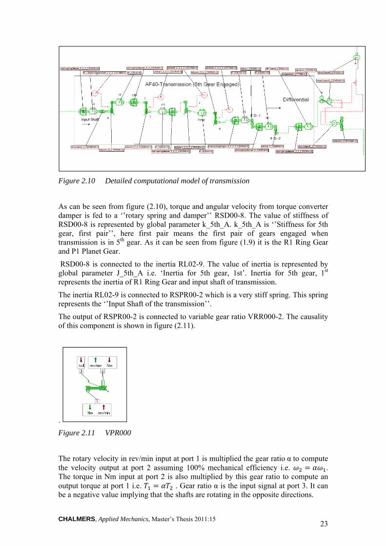
The transmission is modeled as the fifth gear engaged and components used are shown in the figure (2.10).
CHALMERS, Applied Mechanics, Master’s Thesis 2011:15 23
Figure 2.10 Detailed computational model of transmission
As can be seen from figure (2.10), torque and angular velocity from torque converter damper is fed to a ‘’rotary spring and damper’’ RSD00-8. The value of stiffness of RSD00-8 is represented by global parameter k_5th_A. k_5th_A is ‘’Stiffness for 5th gear, first pair’’, here first pair means the first pair of gears engaged when transmission is in 5th gear. As it can be seen from figure (1.9) it is the R1 Ring Gear and P1 Planet Gear.
RSD00-8 is connected to the inertia RL02-9. The value of inertia is represented by global parameter J_5th_A i.e. ‘Inertia for 5th gear, 1st’. Inertia for 5th gear, 1st represents the inertia of R1 Ring Gear and input shaft of transmission.
The inertia RL02-9 is connected to RSPR00-2 which is a very stiff spring. This spring represents the ‘’Input Shaft of the transmission’’.
The output of RSPR00-2 is connected to variable gear ratio VRR000-2. The causality of this component is shown in figure (2.11).
.
Figure 2.11 VPR000
The rotary velocity in rev/min input at port 1 is multiplied the gear ratio α to compute the velocity output at port 2 assuming 100% mechanical efficiency i.e. . The torque in Nm input at port 2 is also multiplied by this gear ratio to compute an output torque at port 1 i.e. . Gear ratio α is the input signal at port 3. It can be a negative value implying that the shafts are rotating in the opposite directions.

CHALMERS, Applied Mechanics, Master’s Thesis 2011:15 24
The input gear ratio applied to -i_5th_A where i_5th_A is the global parameter called ‘’Ratio for 5th gear, first pair’’. The ratio is 17/81 which is gear ratio between R1 Ring Gear and P1 Planet Gear from table (1.2).
The output of VRR000-2 is connected to RL02-6, which is inertia of the P1 Planet Gear. Its notation is J_5th_B.
Output of RL02-6 is connected to RSD00-7. The stiffness is k_5th_B i.e. ‘Stiffness for 5th gear, second pair’. The second pair is the P1 Planet Gear and S2 Sun Gear. The output of RSD00-7 is fed to port 1 of VPR001-1. This component is same as VRR000-2 except for the fact that causality at ports 1 and 2 are interchanged as shown in figure (2.12).
Figure 2.12 VPR001
The rest of the relations and aspects are identical to VRR000-2. The gear ratio α input to VPR001-1 is -i_5th_B which is the global parameter representing ‘’Ratio for 5th gear, second pair’’ and its value is 33/17which represents the pair P1 Planet Gear and S2 Sun Gear. The output of VRR001-1 is connected to inertia RL02-7 representing the inertia of the S2 Sun Gear, its value is represented by J_5th_C. The output of RL02-7 is connected to rotary spring damper RSD00-6, which represents the stiffness k_5th_C and damping. K_5th_C is the ‘Stiffness for 5th gear, third pair’, third pair according to figure (1.9) is gear system between S2 sun Gear and Planet Gear P3.2.
The output of RSD00-6 is connected to variable gear ratio VRR001-2, whose gear ratio α is -i_5th_C i.e. Ratio for 5th gear, third pair whose value is 17/33. A worth mentioning point here is that the ratio here represents not just a gear pair but the system between S2 Sun Gear and P3.2 Planet Gear as explained in the section (1.4.4.2). The output of VRR001-2 is connected to inertia RL02-8 whose notation is J_5th_D. This inertia represents the inertia of the gear system between P3.2 Planet Gear and R3 Ring Gear.
The output of RL02-8 is connected to VPR000-1, its gear ratio α is -i_5th_D= -ve of ‘Ratio for 5th gear, fourth pair’. The fourth pair here is P3.2 Planet Gear and R3 Ring Gear. The output of RSD00-5 is connected to inertia RL02-12 representing the inertia of R3 Ring Gear. Its value is represented by J_5th_E.
The output of RL02-12 is connected to gear ratio RN001-2. The causality and ports of this component are shown in the figure below.

CHALMERS, Applied Mechanics, Master’s Thesis 2011:15 25
Figure2.13 RN001
The gear ratio α of this component is fixed and is input as a real parameter. The rotary velocity port 1 is multiplied the gear ratio α to compute the velocity output at port 2 assuming 100% mechanical efficiency i.e. and torque at port 2 is also multiplied by this gear ratio to compute an output torque at port 1 i.e. . For RN001-2 α is -1/i_5th_E which is –ve inverse of Ratio for 5th gear, fifth pair = 0.906. This as shown by table (1.2) represents R3 Ring Gear is driving the Counter Drive Gear. RSD00-9 represents the stiffness and damping of the gear pair of R3 Ring Gear and Counter Drive Gear. Its stiffness is k_5th_E i.e. Stiffness for 5th gear. The RL02-10 at the output of RSD00-9 represents the inertia of Counter Drive gear and is represented by J_5th_F.
The output of RL02-10 is connected gear ratio, RN000-1. The gear ratio α of RN000-1 is -1/idiff which is negative inverse of ‘’idiff=ratio final drive’’=3.2. The ratio indicates from table (1.2) that Differential Ring Gear is driven by Counter Drive Gear.
RSD0010 represents the damping of the differential pair. Its output is connected to inertia RL02-12 and its represents the inertia of differential gear. The output of RL02-12 is the torque and angular velocity output from transmission. As it can be seen from figure (2.10) the torque is divided between two side shafts by RCON00-1. The causality and ports of this component are shown in the figure (2.14).
Figure 2.14 RCON00
The equations for this component are T3=T2+T1 and ω1= ω2= ω3.
Also the torque from transmission is fed to the power train mounts by TWSG02-1 whose angular velocity as can be seen from figure (2.10) is sunk.

CHALMERS, Applied Mechanics, Master’s Thesis 2011:15 26
2.1.4 Side Shafts
The input to the side shafts are angular velocity and torque from transmission and at their output wheels are connected.
In the model there are two output shafts and they are equivalent in every aspect. Since the model does not exhibits the turning maneuver etc so the torque distribution at RCON00-1 in figure (2.10) is such that T3=T2+T1 where T2=T1.
Figure (2.15) shows the detailed model of side shaft. The model only describes the inertia of the shaft by RL01. The rotary clearance MCCL0A defines the clearance of shaft. The stiffness of shaft is defined by RSD000.
Figure 2.15 Detailed model of side shaft
2.1.5 Mechatronic Clutch
As already explained in the section (1.5.1), the components of mechatronic clutch should be connected according to the figure (1.11). The section (2.1.2) explains the torque converter damper and lock-up clutch connected in parallel, which does not replicate the physical system. So this configuration needs to be changed. The mechatronic clutch system according to the conventional layout in the figure (1.11) is shown below:

CHALMERS, Applied Mechanics, Master’s Thesis 2011:15 27
Figure 2.16 Mechatronic Clutch System
The above figure shows that lock-up clutch and TCC damper are connected in series and both of them are connected in parallel with dynamic torque converter. This revised model also contains crank shaft without inertia as shown in the figure 2.17.
Figure 2.17 Crank Shaft
The stiffness and damping of the crank shaft are set such that they don’t affect the torque and velocity profile coming from the engine. Also the relative angular displacement is zero up to two decimal places. The stiffness is set to 100000 Nm/deg and damping is set to 10000 Nm/(rev/min). The reason of adding the crank shaft is to change the causality of the system.

CHALMERS, Applied Mechanics, Master’s Thesis 2011:15 28
3 Verification
The computational model of a Mechatronic Clutch System needs to be verified before going to the next phase of the project. The purpose of verification is to check whether the system fulfils its specification or not. The main focus is concentrated on verifying the desired behavior qualitatively. The Mechatronic clutch system is verified in two steps.
1. Dynamic Torque Converter 2. Mechatronic Clutch (Torque Converter, TCC Damper, Lock-up Clutch)
3.1 Torque converter For this purpose, a test jig has been developed in AMESim as shown in the figure (3.1). A torque profile is given as an input to the torque converter and a rotary spring damper and a rotary load is connected at its output along with torque and rotary speed sensors.
Figure 3.1 Torque Converter Test Jig
The input torque profile is shown in figure (3.2). The torque is zero for the first five seconds, then given a step of 100 for next 30 seconds, then 200 for 25 seconds. It is then lowered to -200 for 25 seconds which is not a practical scenario but it has been generated to verify a particular mode of torque converter. The signal is then raised to 100 till end.
Figure (3.3) shows torque on impeller and turbine. The impeller and input torque are same but torque on turbine shows different behavior. A sudden increase in amplitude of turbine torque at every step shows torque multiplication. When the input torque becomes constant means the vehicle is running in a highway or with constant speed, both the torques become equal which explain the coupling phenomena. Engine never generates negative torque in a practical scenario, but here it is generated to observe the overrun mode of the torque converter in which the transmission drives the engine to generate braking torque.

CHALMERS, Applied Mechanics, Master’s Thesis 2011:15 29
Figure 3.2 Input Torque
Figure 3.3 Torque on Impeller (red) and Turbine (green)
Torque ratio is represented in figure (3.4). The noticeable point is when the torque ratio becomes less than 1. This point represents the overrun mode which has been explained earlier.
At steady state, torque converter transmits all the torque coming from the engine but with some losses due to fluid coupling within the torque converter. The losses are observable by comparing the rotary velocities of impeller and turbine as shown in figure (3.5). It is clearly visible that the turbine rotary velocity never reached impeller rotary velocity. Moreover, the turbine velocity increases smoothly during vehicle launch which is one of the characteristics of torque converter.

CHALMERS, Applied Mechanics, Master’s Thesis 2011:15 30
Figure 3.4 Torque Ratio
Figure 3.5 Impeller and Turbine rotary velocity
Figure (3.6) shows velocity ratio graph. Two big spikes are due to the sudden and big changes in the input torque which is not a practical scenario. The remaining behavior is logical and closer to reality. In the beginning, it is zero then increases gradually and at last reaches at 1.
The stator is locked via one way clutch during torque multiplication and free to move along with impeller and turbine during coupling mode. In other words, the stator should experience torque during torque multiplication mode and zero torque during coupling mode. The behavior seems practical as shown in the figure (3.7) which shows that the torque on the stator is zero after 105 seconds which is also the point of coupling mode. The torque becomes zero at the 60th second because rotation of the turbine changes its direction at that point. The coupling also occurs between 60 and 70 seconds and verified by zero torque on stator in that duration.

CHALMERS, Applied Mechanics, Master’s Thesis 2011:15 31
Figure 3.6 Velocity Ratio
Figure 3.7 Torque on stator due to one way clutch
The stator rotates along with impeller and turbine in the coupling mode which can be seen in the figure (3.8).
Figure (3.9) shows volumetric flow rate of fluid in tore. The main reason to see this graph is to verify the direction of flow during overrun mode. The figure clearly explains that the flow changes its direction during overrun mode.

CHALMERS, Applied Mechanics, Master’s Thesis 2011:15 32
Figure 3.8 Stator rotary velocity
Figure 3.9 Volumetric flow rate in tore
3.2 Mechatronic Clutch
The section 2.1.5 explains briefly about the mechatronic clutch. The verification of the system will be done by the critical analysis of system response when:
1. lock-up clutch is fully disengaged 2. lock-up clutch is partially engaged 3. lock-up clutch is fully engaged
The system response will be then compared with the actual response qualitatively.
CHALMERS, Applied Mechanics, Master’s Thesis 2011:15 33
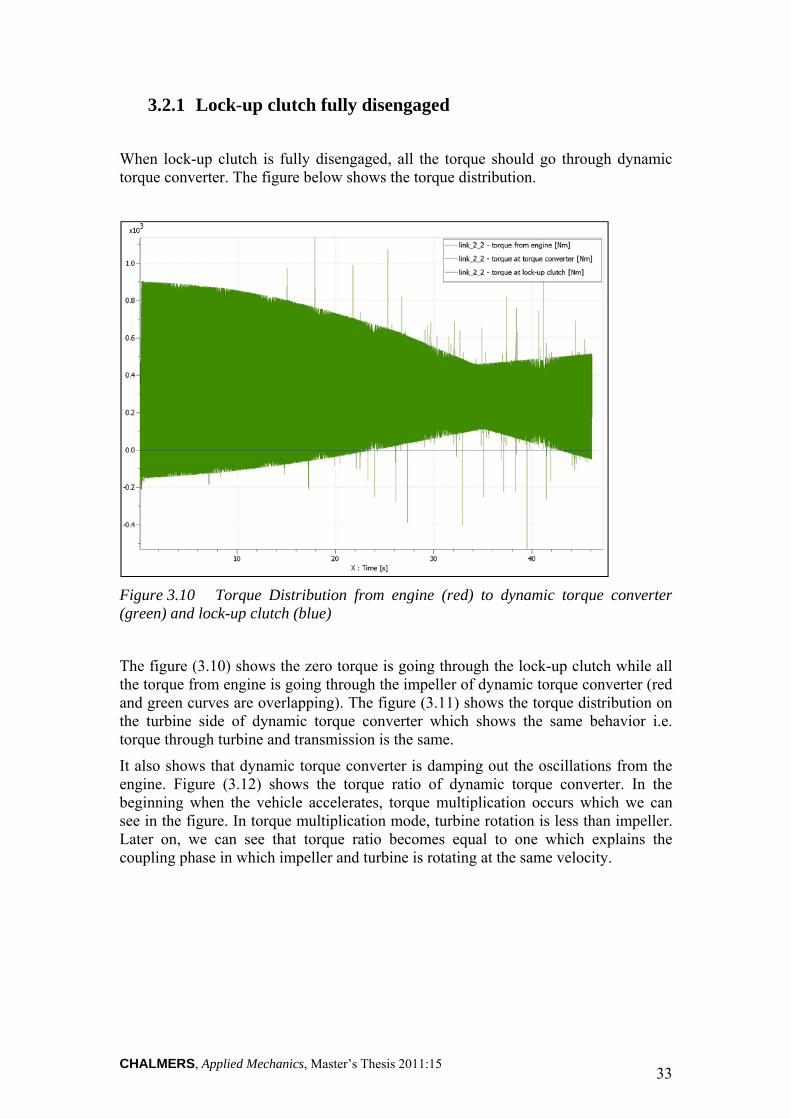
3.2.1 Lock-up clutch fully disengaged
When lock-up clutch is fully disengaged, all the torque should go through dynamic torque converter. The figure below shows the torque distribution.
Figure 3.10 Torque Distribution from engine (red) to dynamic torque converter (green) and lock-up clutch (blue)
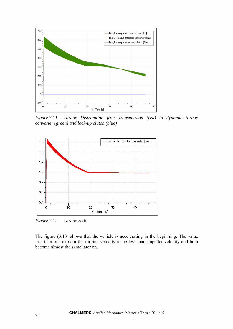
The figure (3.10) shows the zero torque is going through the lock-up clutch while all the torque from engine is going through the impeller of dynamic torque converter (red and green curves are overlapping). The figure (3.11) shows the torque distribution on the turbine side of dynamic torque converter which shows the same behavior i.e. torque through turbine and transmission is the same.
It also shows that dynamic torque converter is damping out the oscillations from the engine. Figure (3.12) shows the torque ratio of dynamic torque converter. In the beginning when the vehicle accelerates, torque multiplication occurs which we can see in the figure. In torque multiplication mode, turbine rotation is less than impeller. Later on, we can see that torque ratio becomes equal to one which explains the coupling phase in which impeller and turbine is rotating at the same velocity.
CHALMERS, Applied Mechanics, Master’s Thesis 2011:15 34
Figure 3.11 Torque Distribution from transmission (red) to dynamic torque converter (green) and lock-up clutch (blue)
Figure 3.12 Torque ratio
The figure (3.13) shows that the vehicle is accelerating in the beginning. The value less than one explain the turbine velocity to be less than impeller velocity and both become almost the same later on.

CHALMERS, Applied Mechanics, Master’s Thesis 2011:15 35
Figure 3.13 Velocity ratio
Figure (3.14) explains the fluid coupling loss which causes the turbine velocity to be less than impeller velocity thus decreasing the fuel efficiency of the vehicle. But on the other hand, it is increasing the comfort level of the passenger.
Figure 3.14 Impeller and turbine rotary velocity
3.2.2 Lock-up clutch partially engaged
The lock-up clutch is given a control signal as shown in the figure (3.15) to investigate the behavior of mechatronic clutch. The clutch is kept open for the first 10 seconds, closes up to 50% in next 2 seconds and then kept at this position for entire 48 seconds.

CHALMERS, Applied Mechanics, Master’s Thesis 2011:15 36
Figure 3.15 Lock-up clutch control signal
Figure (3.16) shows the torque distribution from engine to dynamic torque converter and lock-up clutch. The torque through dynamic torque converter is the same as that of engine in the first 10 seconds because of the open clutch. As soon as the clutch closes partially, the torque from engine splits into the dynamic torque converter and lock-up clutch. The natural damping action of lock-up clutch is also clearly visible in the figure. Figure (3.17) shows the torque distribution from the transmission side which have the similar response. The plot is self explanatory as the torque spikes are very much damped out through the mechatronic clutch.
Figure 3.16 Torque Distribution from engine (red) to dynamic torque converter (green) and lock-up clutch (blue)
CHALMERS, Applied Mechanics, Master’s Thesis 2011:15 37
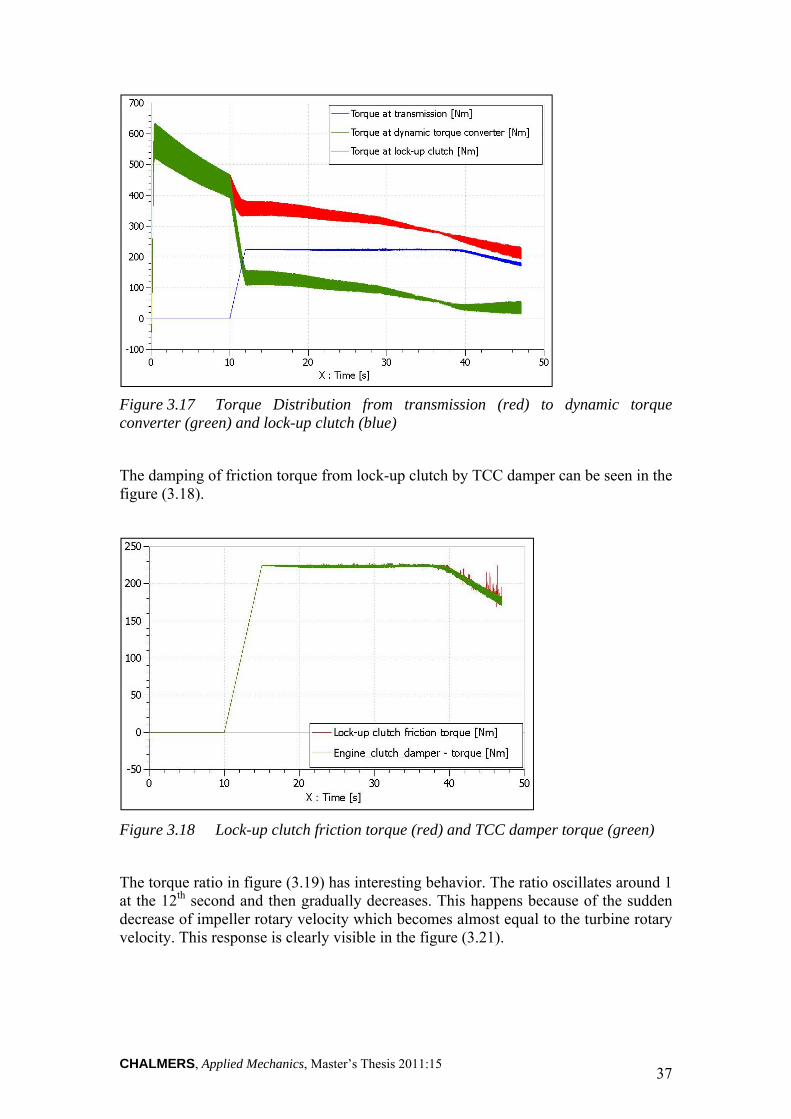
Figure 3.17 Torque Distribution from transmission (red) to dynamic torque converter (green) and lock-up clutch (blue)
The damping of friction torque from lock-up clutch by TCC damper can be seen in the figure (3.18).
Figure 3.18 Lock-up clutch friction torque (red) and TCC damper torque (green)
The torque ratio in figure (3.19) has interesting behavior. The ratio oscillates around 1 at the 12th second and then gradually decreases. This happens because of the sudden decrease of impeller rotary velocity which becomes almost equal to the turbine rotary velocity. This response is clearly visible in the figure (3.21).

CHALMERS, Applied Mechanics, Master’s Thesis 2011:15 38
Figure 3.19 Torque ratio
Velocity ratio has expected behavior i.e. opposite to the torque ratio until 12th second and then approaches 1 gradually.
Figure 3.20 Velocity ratio
During torque multiplication, turbine rotary velocity is less than impeller rotary velocity and when lock-up clutch partially engages the vehicle starts to cruise as shown in the figure (3.21).

CHALMERS, Applied Mechanics, Master’s Thesis 2011:15 39
Figure 3.21 Impeller and turbine rotary velocity
3.2.3 Lock-up clutch fully engaged
The lock-up clutch is fully closed for 60 seconds i.e. given a control signal 1. As explained in the section (1.5.2) when lock-up clutch is fully engaged, all the torque should go through the lock-up clutch, TCC damper and turbine of dynamic torque converter. But the behavior is a bit different as shown in the figure (3.22) below:
Figure 3.22 Torque Distribution from engine (red) to dynamic torque converter (green) and lock-up clutch (blue)
CHALMERS, Applied Mechanics, Master’s Thesis 2011:15 40
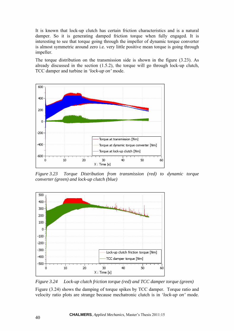
It is known that lock-up clutch has certain friction characteristics and is a natural damper. So it is generating damped friction torque when fully engaged. It is interesting to see that torque going through the impeller of dynamic torque converter is almost symmetric around zero i.e. very little positive mean torque is going through impeller.
The torque distribution on the transmission side is shown in the figure (3.23). As already discussed in the section (1.5.2), the torque will go through lock-up clutch, TCC damper and turbine in ‘lock-up on’ mode.
Figure 3.23 Torque Distribution from transmission (red) to dynamic torque converter (green) and lock-up clutch (blue)
Figure 3.24 Lock-up clutch friction torque (red) and TCC damper torque (green)
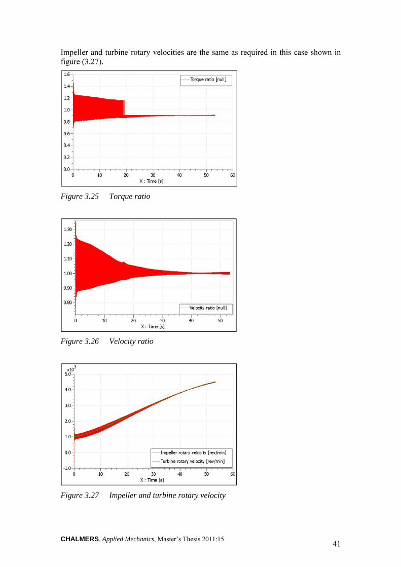
Figure (3.24) shows the damping of torque spikes by TCC damper. Torque ratio and velocity ratio plots are strange because mechatronic clutch is in ‘lock-up on’ mode.
CHALMERS, Applied Mechanics, Master’s Thesis 2011:15 41
Impeller and turbine rotary velocities are the same as required in this case shown in figure (3.27).
Figure 3.25 Torque ratio
Figure 3.26 Velocity ratio
Figure 3.27 Impeller and turbine rotary velocity

CHALMERS, Applied Mechanics, Master’s Thesis 2011:15 42
4 Validation
To determine whether the model is accurately representing the real system is known as validation. The main goal is to make the model useful in a sense that the model addresses the right problem, provides accurate information about the system being modeled. It is usually achieved through comparing the model with actual system behavior and using the discrepancies between the two, and the insights gained, to improve the model. The process is repeated until the model accuracy becomes acceptable.
The validation starts with post processing of simulation results. The simulation results obtained from AMESim model are post processed in MATLAB to get:
Acceleration of engine, transmission input shaft, differentials, and rim of wheel in rad/s2 over the entire speed
Damping in dB related to 1 deg/s for engine to differential Damping in dB related to 1 deg/s for engine to rim
The virtual validation is done because engine needs to be controlled in order to generate same output as the original system which is not in the scope of this thesis work. Virtual validation is done by the comparison of post processed simulation results between further developed model and by removing dynamic torque converter from that model. The input from engine (Bounds on input) is very important for validation of whole system response.
The plots below are the 2nd order responses of further developed AMESim model with complete mechatronic clutch in ‘lock-up on’ mode:
Figure 4.1 Acceleration of engine (rad/s2)

CHALMERS, Applied Mechanics, Master’s Thesis 2011:15 43
Figure 4.2 Acceleration of input shaft (rad/s2)
Figure 4.3 Acceleration of differential (rad/s2)

CHALMERS, Applied Mechanics, Master’s Thesis 2011:15 44
Figure 4.4 Acceleration of rim of wheel (rad/s2)
Figure 4.5 Isolation from engine to differential db (rel. 1 deg/s)
The acceleration profiles at input shaft, differentials and at rim of the wheel shows the damping of signals. Acceleration at rim of wheel goes below 40 rad/s2 or 20 db at 1400 rpm as shown in figures (4.4) and (4.6).

CHALMERS, Applied Mechanics, Master’s Thesis 2011:15 45
Figure 4.6 Isolation from engine to rim db (rel. 1 deg/s)
The figure (4.7) shows the mechatronic clutch without dynamic torque converter but with impeller inertia added into the engine inertia and turbine, stator and oil inertias added after TCC damper as can be seen in the figure below.
Figure 4.7 Mechatronic clutch with only dynamic torque converter inertias
The acceleration and damping profiles of the system are given below:
CHALMERS, Applied Mechanics, Master’s Thesis 2011:15 46
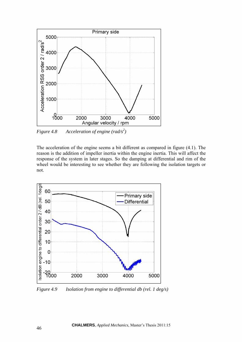
Figure 4.8 Acceleration of engine (rad/s2)
The acceleration of the engine seems a bit different as compared in figure (4.1). The reason is the addition of impeller inertia within the engine inertia. This will affect the response of the system in later stages. So the damping at differential and rim of the wheel would be interesting to see whether they are following the isolation targets or not.
Figure 4.9 Isolation from engine to differential db (rel. 1 deg/s)

CHALMERS, Applied Mechanics, Master’s Thesis 2011:15 47
Figure (4.9) shows that further developed model at differentials is damping out a bit more than model without dynamic torque converter. This is because of the low mean torque going through the dynamic torque converter. However, response at rim of the wheel is almost same as previous as shown in figures (4.6) and (4.10). The only difference is the transients in the rim curve till the end in the figure (4.6). No conclusions can be made on this behavior because the input from the engine is different in both cases. However, this is a minor difference and can be neglected because the system is far from the critical zone (damping is less than zero).
Figure 4.10 Isolation from engine to rim db (rel. 1 deg/s)
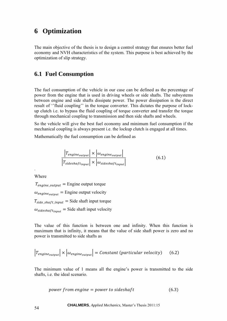
Now the slip is introduced in the mechatronic clutch to see the damping behavior. The lock-up clutch is kept at 35% closed position for whole simulation; the following slip profile is obtained as shown in the figure (4.11). The figures (4.12) and (4.13) show the improved damping at differential and rim of the wheel. However, the slip profile seems to have very high values. The reason is high acceleration input from the engine.
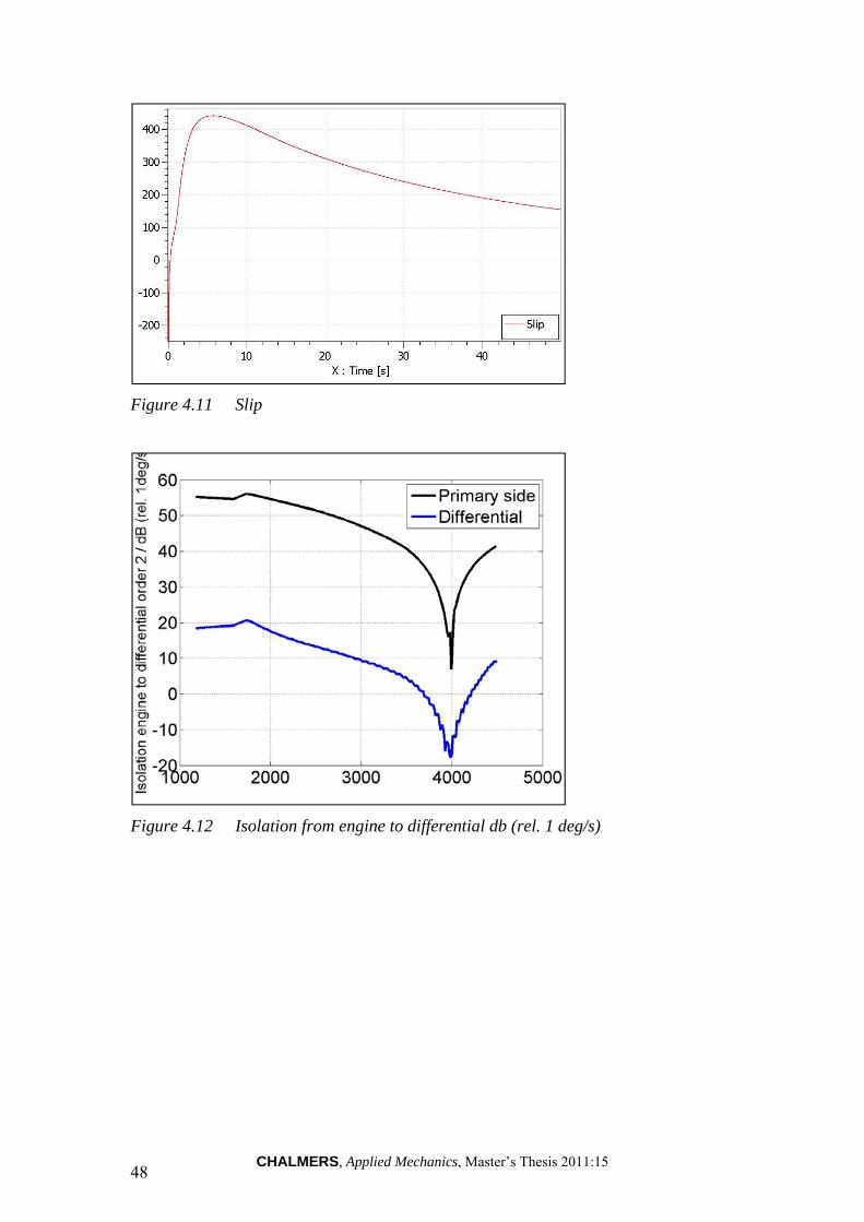
CHALMERS, Applied Mechanics, Master’s Thesis 2011:15 48
Figure 4.11 Slip
Figure 4.12 Isolation from engine to differential db (rel. 1 deg/s)

CHALMERS, Applied Mechanics, Master’s Thesis 2011:15 49
Figure 4.13 Isolation from engine to rim db (rel. 1 deg/s)
All the tests are satisfying the correct model behavior. However, the quantitative validation can be done if actual data as well as physical parameters of dynamic torque converter are available.

CHALMERS, Applied Mechanics, Master’s Thesis 2011:15 50
5 ECCC Slip Control Strategy
The purpose of slip control strategy or ECCC slip strategy is to ensure that the mechatronic clutch maintains a constant slip over a speed range hence ensuring minimum vibrations and maximum fuel efficiency at that particular speed and driving condition. The controller as applied in the AMESim model is shown in figure (5.1).
Figure 5.1 PID Controller
The controller is designed in the simplest possible manner keeping in view its application platform and minimum requirements.
5.1 Working principle of slip controller
The working principle of slip controller is that the torque coming from the engine has to be distributed between torque converter and torque converter damper by opening and closing the clutch. The torque ratio going to the torque converter decides the speed difference between the impeller (on engine side) and turbine (on transmission side) i.e.
5.1
When the clutch is fully locked the slip is equal to zero. The controller does not takes that case into account and shuts itself down if the ‘’REQUIRED SLIP’’ is zero. On all the other values the controller opens and closes clutch in order to maintain the required slip.

CHALMERS, Applied Mechanics, Master’s Thesis 2011:15 51
5.1.1 Control loop
First the current speed of impeller and turbine are measured by two speed sensors as shown in figure (5.1). The ‘function blocks’ f(x) take the absolute of these values and the ‘mean blocks’ remove any non realistic instantaneous values to provide a smooth output. The two smoothed speed signals are subtracted to get the current slip.
The division operator is used to determine the
5.2
The error ratio is equal to 1 if the current slip and required slip are equal. The error ratio is subtracted from 1 to make normalized error
1 5.3
Feedback loop of controller is designed in such a way because the clutch model available takes the input command between zero and one. Zero corresponding to a fully open and one corresponding to fully locked clutch.
The normalized error is then fed to a PI controller with P=1 and I=0.5. These values can be adjusted in actual model by using any available PI tuning algorithm and some test runs. For this thesis we tuned the controller by manual tuning.
The output of the controller after passing through the saturation element with bounds zero and one is fed to the clutch.
5.1.2 Output characteristics of controller
The controller successfully regulates the value of slip for 1 to 60 rpm. The control error is always below 0.3 rpm and is in accordance to specification from SAAB which is 0.5 rpm.
For the control operation, the data presented below is from speed of 900 rpm to 1600 rpm varying linearly in 14 seconds. The slip to be maintained is 50 rpm. The required slip (green) and current slip (red) for the above speed is shown in the figure (5.2).

CHALMERS, Applied Mechanics, Master’s Thesis 2011:15 52
Figure 5.2 Required and current slip profiles
The control error is shown in the figure (5.3). As can be seen from figure the error is always less than +0.3 rpm.
Figure 5.3 Control error
The input signal to the clutch is shown in the figure (5.4). As can be seen from signal the clutch is continuously pressed and released to maintain the required slip.

CHALMERS, Applied Mechanics, Master’s Thesis 2011:15 53
Figure 5.3 Control signal of the lock-up clutch
CHALMERS, Applied Mechanics, Master’s Thesis 2011:15 54
6 Optimization
The main objective of the thesis is to design a control strategy that ensures better fuel economy and NVH characteristics of the system. This purpose is best achieved by the optimization of slip strategy.
6.1 Fuel Consumption
The fuel consumption of the vehicle in our case can be defined as the percentage of power from the engine that is used in driving wheels or side shafts. The subsystems between engine and side shafts dissipate power. The power dissipation is the direct result of ‘’fluid coupling’’ in the torque converter. This dictates the purpose of lock-up clutch i.e. to bypass the fluid coupling of torque converter and transfer the torque through mechanical coupling to transmission and then side shafts and wheels.
So the vehicle will give the best fuel economy and minimum fuel consumption if the mechanical coupling is always present i.e. the lockup clutch is engaged at all times.
Mathematically the fuel consumption can be defined as
6.1
.
Where
_ Engine output torque
Engine output velocity
_ _ Side shaft input torque
Side shaft input velocity
The value of this function is between one and infinity. When this function is maximum that is infinity, it means that the value of side shaft power is zero and no power is transmitted to side shafts as
6.2
The minimum value of 1 means all the engine’s power is transmitted to the side shafts, i.e. the ideal scenario.
6.3

CHALMERS, Applied Mechanics, Master’s Thesis 2011:15 55
6.2 NVH characteristics
The NVH characteristic of the vehicle in our case is defined as the ratio of the angular acceleration of the side shaft to the angular acceleration of engines output or it can be the ratio between acceleration of side shaft and some constant angular acceleration that defines the threshold value of NVH characteristic acceptable. The subsystem that decreases the acceleration from engine to side shafts most is the fluid coupling of torque converter as it has an intrinsic damping characteristic. The acceleration of side shaft is most i.e. equal to that of the engine when the mechanical coupling or lock up clutch is engaged. So the vehicle gives the best fuel economy if the mechanical coupling is engaged all the time.
Mathematically NVH characteristic can be defined as
, 6.3
Or
, 6.4
Where
_ _ Angular acceleration of side shaft at present time t
_ Angular acceleration of engine at present time t
_ Max acceleration defined for acceptable NVH characteristic
The value of this function is between zero and one. Where zero suggests that the angular acceleration of side shafts is zero and the systems damping is very ideal. Value of 1 indicates that either the acceleration of side shaft is equal to that of engine or the predefined limit.
6.3 Conflicting Criterion
As can be seen from equations (6.1) and (6.2) minimization of the two functions at the same time is not possible. Fuel economy requires maximum mechanical coupling while better NVH characteristics require maximum fluid coupling, which cannot be achieved simultaneously.
This makes the problem a multi objective optimization problem. The treatment of such problems requires the use of evolutionary algorithms such as ‘Genetic Algorithm’ for the minimization of multi objective function.
The best feature of this algorithm is the fact that it does not assign weights to the individual objective function, as is done by conventional optimization techniques. This ensures that the result generated by the genetic algorithm is optimal in a global

CHALMERS, Applied Mechanics, Master’s Thesis 2011:15 56
sense and not weight dependent. Also genetic algorithm produces Pareto front and Pareto set. The Pareto front gives the value of objective functions and Pareto set gives the value of input for the points in Pareto front. These values are optimal meaning that the better result cannot be achieved.
6.4 Optimization approach
For our model the optimization algorithm is represented by following flow chart.
6.4.1 AMESim model
The AMESim model used in optimization algorithms is exactly same as our new model with the additional interface block called SimuCosim. In Simulink-AMESim co-simulation interface, both programs use their own solvers and only exchange inputs and outputs as shown in figure (6.1) taken from the AMESim and Simulink user manual.
Figure 6.1 Co-simulation interface
Input Slip
Velocity range
Optimization tool box in MATLAB
Fitness function in Matlab
Simulink
Model
AMESim
Model
Input slip from genetic algorithm
Value of NVH and FUEL economy at a particular velocity range
Velocity range at which the objective functions are to be
optimized
Input Slip Values of NVH and FUEL economy for a complete predefined velocity sweep
Values of NVH and FUEL economy for a complete predefined velocity sweep

CHALMERS, Applied Mechanics, Master’s Thesis 2011:15 57
The interface block in our model is shown in figure (6.2)
Figure 6.2 Interface block
In one complete cycle the complete driveline model i.e. our AMESim model takes the input of ‘slip’ from ‘co-simulation Interface’. Then it runs the complete simulation of the time, sampling time and other options set by AMESim and when the simulation is complete, it sends the data to ‘co-simulation Interface’ and waits for the next value of slip to evaluate.
6.4.2 Simulink model
The interface block is accessible by Simulink by S-function. The AMESim compiler changes the co-simulation Interface into a C code and that code is exactly read by the S-function in Simulink.
Figure 6.3 Simulink model
6.4.3 Fitness Function
Fitness function in Matlab is defined as ‘the evaluation function for genetic algorithm’. It means that it takes the value of input, in our case the ‘slip’ and gives the value of output, in our case the value of NVH and Fuel as the output to genetic algorithm.
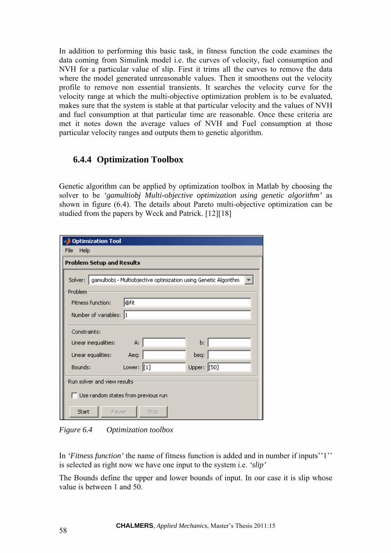
CHALMERS, Applied Mechanics, Master’s Thesis 2011:15 58
In addition to performing this basic task, in fitness function the code examines the data coming from Simulink model i.e. the curves of velocity, fuel consumption and NVH for a particular value of slip. First it trims all the curves to remove the data where the model generated unreasonable values. Then it smoothens out the velocity profile to remove non essential transients. It searches the velocity curve for the velocity range at which the multi-objective optimization problem is to be evaluated, makes sure that the system is stable at that particular velocity and the values of NVH and fuel consumption at that particular time are reasonable. Once these criteria are met it notes down the average values of NVH and Fuel consumption at those particular velocity ranges and outputs them to genetic algorithm.
6.4.4 Optimization Toolbox
Genetic algorithm can be applied by optimization toolbox in Matlab by choosing the solver to be ‘gamultiobj Multi-objective optimization using genetic algorithm’ as shown in figure (6.4). The details about Pareto multi-objective optimization can be studied from the papers by Weck and Patrick. [12][18]
Figure 6.4 Optimization toolbox
In ‘Fitness function’ the name of fitness function is added and in number if inputs’’1’’ is selected as right now we have one input to the system i.e. ‘slip’
The Bounds define the upper and lower bounds of input. In our case it is slip whose value is between 1 and 50.

CHALMERS, Applied Mechanics, Master’s Thesis 2011:15 59
The toolbox also allows to set the options for genetic algorithm e.g. population size, initial population, stopping criterion etc.
Once all the options are set and optimization is started, in first run the toolbox gives fitness function a random value of slip and a value of NVH and fuel consumption is returned by fitness function based on AMESim model and calculated by AMESim solver. Genetic algorithm then sends another value of slip and the cycle goes on until one of the conditions in stopping criterion is fulfilled and the output is values of slip for which at a particular velocity we have the minimized NVH and fuel consumption.
The values of slip are plotted in a Pareto set and values of NVH and fuel consumption are plotted in a Pareto front.
6.5 Results from optimization The optimization was done for various mean engine velocity ranges. The value of slip is from 1 rpm to 50 rpm. The values of slip i.e. Pareto set are shown along with their corresponding points in Pareto front. The min fuel consumption and min NVH possible at each velocity range is also given, in order to establish the sense of optimization. These minimum values are based on original model.
The genetic algorithm is set to the population size of 8, and 15 generations as the stopping criteria.
The results for the velocity range 1250 to 1260 rpm is shown in figure (6.5). At clutch fully locked the value of fuel consumption is 2.0085 and at max slip i.e. 50 rpm the value of NVH is 0.0307.
Figure 6.5 Pareto front for the speed range of 125-1260 rpm

CHALMERS, Applied Mechanics, Master’s Thesis 2011:15 60
The Pareto front for the velocity range of 1280 to 1290 rpm is shown in figure (6.6). Minimum value of fuel consumption 2.0095 i.e. at clutch fully locked is and min value of NVH i.e. at slip of 50 rpm is 0.0292.
Figure 6.6 Pareto front for the speed range of 1280-1290 rpm
At velocity range of 1300 to 1310 rpm, the Pareto front is shown in figure (6.7).Min fuel consumption is 2.0101 and min NVH is 0.0284
Figure 6.7 Pareto front for the speed range of 1300-1310 rpm

CHALMERS, Applied Mechanics, Master’s Thesis 2011:15 61
The optimization result of velocity range of 1350 to 1360 rpm is shown in figure (6.8). Min fuel consumption for this velocity range is 2.0113 and min NVH is 0.0267.
Figure 6.8 Pareto front for the speed range of 1350-1360 rpm
Figure 6.9 Pareto front for the speed range of 1380-1390 rpm
Pareto front for the velocity range of 1380 to 1390 rpm is shown in figure (6.9). Min fuel consumption for this velocity range is 2.0119. Min NVH is 0.0259 which is less than the points for points corresponding to the slip of 47.5 and 48.5 which are 0.0273 and 0.0267 respectively.

CHALMERS, Applied Mechanics, Master’s Thesis 2011:15 62
6.6 Discussion on results
The results of optimization show the Pareto fronts which exactly show the optimized solutions to our multi-objective criterion. These solutions can be made more ‘optimal’ if we run the genetic algorithm for more generations.
This possibility was explored by running the simulation for the velocity range of 1380 to 1390 again for 30 generations and now the result is supposed to be more optimal than the one with 15 generations.
Figure 6.10 Comparison of same objective function evaluated by different generation limits
Figure (6.10) shows the optimization results for both 15 generation limit (magenta curve) and 30 generation limit (red curve).
As we can see in the figure, extreme points of the two curves almost overlay, emphasizing on the fact that, increasing the number of generations has little effect on the extreme points. Also for the intermediate points the Pareto fronts are close and even intersect each other. Due to this closeness in the pareto fronts we can conclude that running the optimization with 15 generations is less accurate but acceptable as it takes half the computational time as compared to that with 30 generations.
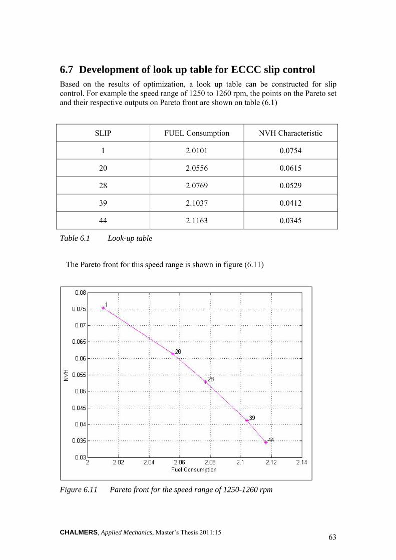
CHALMERS, Applied Mechanics, Master’s Thesis 2011:15 63
6.7 Development of look up table for ECCC slip control Based on the results of optimization, a look up table can be constructed for slip control. For example the speed range of 1250 to 1260 rpm, the points on the Pareto set and their respective outputs on Pareto front are shown on table (6.1)
SLIP FUEL Consumption NVH Characteristic
1 2.0101 0.0754
20 2.0556 0.0615
28 2.0769 0.0529
39 2.1037 0.0412
44 2.1163 0.0345
Table 6.1 Look-up table
The Pareto front for this speed range is shown in figure (6.11)
Figure 6.11 Pareto front for the speed range of 1250-1260 rpm

CHALMERS, Applied Mechanics, Master’s Thesis 2011:15 64
If for example we have criteria that the NVH characteristic should be less than 0.04 then we can conclude that there is not a single value of slip less than 44 rpm that can give us the fuel consumption of 2.1163. Also if this NVH criterion is selected then we can never have fuel consumption below 2.1163. So we will set our controller to give a slip of 44 when engine is at this speed range.
Similarly we can set criteria that fuel consumption must be less than 2.0769 and at the same time NVH must be less than 0.0529, then we can say that only a slip of 28 will guarantee this criteria to be satisfied and system will be regulated at this slip whenever it is in the 1250-1260 rpm range.
This leads to a multi-dimensional look up table. On one axis we can choose criteria on NVH and fuel consumption to be followed and the mechatronic clutch will regulate the slip based on the current engine speed to fulfill these criteria.
Similar Pareto fronts on the whole velocity range of vehicle will give a table that shows the value of slip to be regulated at every velocity in order to provide optimum NVH and fuel consumption.
The arrangement of the look up table with the system is shown in figure (6.12)
Figure 6.12 Look up table to relate current engine speed with it’s corresponding optimized slip
6.8 Sensitivity analysis of end-stop angles of TCC Damper
In reference to the figure (2.16), the relative angular displacement when just in contact of 1st and 2nd stage end-stops are changed to analyze the damping of the system. Following notations are used for simplicity:
Relative angular displacement when just in contact of 1st stage end-stop = Phi1
Relative angular displacement when just in contact of 2nd stage end-stop = Phi2
There are four different cases:
1. Phi1 is increased 2. Phi1 is decreased 3. Phi2 is increased 4. Phi2 is decreased
Each case is simulated with batch size of four. Table (6.2) below is showing the values of phi1 and phi2 for the cases mentioned above. For each case, only one variable is changed and the other variable is kept constant.
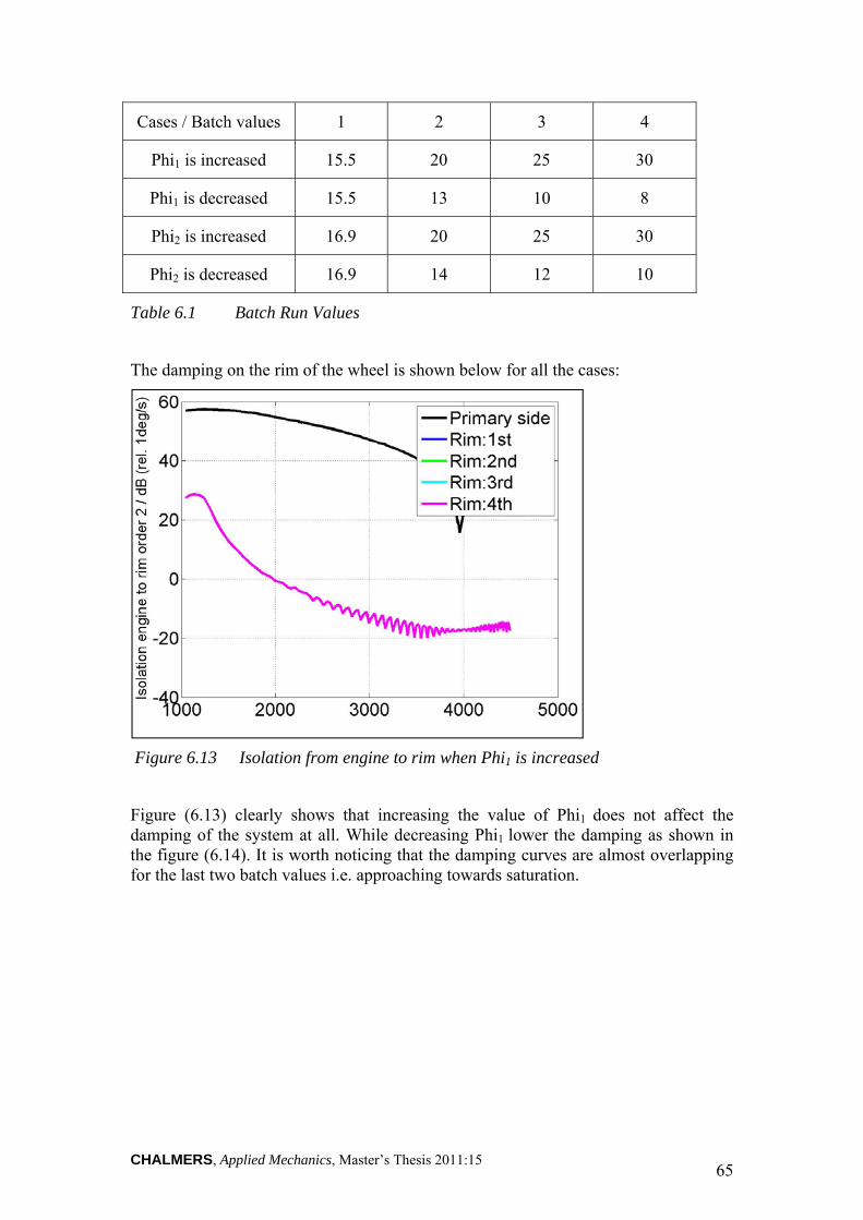
CHALMERS, Applied Mechanics, Master’s Thesis 2011:15 65
Cases / Batch values 1 2 3 4
Phi1 is increased 15.5 20 25 30
Phi1 is decreased 15.5 13 10 8
Phi2 is increased 16.9 20 25 30
Phi2 is decreased 16.9 14 12 10
Table 6.1 Batch Run Values
The damping on the rim of the wheel is shown below for all the cases:
Figure 6.13 Isolation from engine to rim when Phi1 is increased
Figure (6.13) clearly shows that increasing the value of Phi1 does not affect the damping of the system at all. While decreasing Phi1 lower the damping as shown in the figure (6.14). It is worth noticing that the damping curves are almost overlapping for the last two batch values i.e. approaching towards saturation.

CHALMERS, Applied Mechanics, Master’s Thesis 2011:15 66
Figure 6.14 Isolation from engine to rim when Phi1 is decreased
Figure 6.15 Isolation from engine to rim when Phi2 is increased

CHALMERS, Applied Mechanics, Master’s Thesis 2011:15 67
Figure 6.16 Isolation from engine to rim when Phi2 is decreased
Similar is the case when Phi2 is increased i.e. no change in damping. While decreasing Phi2 lower the damping. Similar behavior is seen for last two batch values of Phi2. It is concluded from the above analysis that the present values of Phi1 i.e. 15.5 and Phi2 i.e. 16.9 are the optimal values regarding the damping of the system.
CHALMERS, Applied Mechanics, Master’s Thesis 2011:15 68
7 Conclusion
A mechatronic clutch system has been introduced in already existing complete vehicular driveline model. Previously, the model was working only in ‘lock-up’ mode but now it is applicable to complete stick-slip profile. The controller in mechatronic clutch system regulates the slip within an acceptable error margin. The slip is imported from a ‘look-up table’ based on genetic algorithm which minimizes the NVH and fuel consumption of the vehicle for a particular velocity or a velocity range.
In order to introduce slip in the system, dynamic torque converter has been implemented in the system. The model implemented here is a nonlinear model of hydro-dynamic torque converter that takes into account the transient behavior of the fluid for the complete frequency range of velocity as compared to steady state torque converter model which is applicable to a very narrow frequency range of velocity.
The fuel consumption and NVH are two contradictive objectives in the system considered. To solve the optimization problems with these two criteria several approaches can be used. In this thesis the genetic algorithm is chosen to solve bio-objective optimization The algorithm despite being computationally slow gives the optimized solution on the ‘pareto front’ with respect to ‘pareto set’ of input variables. These solutions are independent of relative weights or importance of individual objectives. Once the optimized ‘pareto set’ is calculated, a look-up table is developed which is then imbedded in the real time system.
For considered problem, the above mentioned objectives are optimized on a particular velocity range for a complete sweep of slip. This procedure gives the value of slip at each velocity instance, the look-up table then only has to read the velocity of the engine and apply it respective slip to the mechatronic clutch hence giving minimum vibrations in the driveline and maximum fuel efficiency of the vehicle.

CHALMERS, Applied Mechanics, Master’s Thesis 2011:15 69
8 Future Work
The control performance can be improved by application of an advanced control algorithm such as LQG (Linear Quadratic Gaussian) control or MPC (Model Predictive Control).
Currently, the engine is taken as an uncontrollable input source. The model can be further developed to have a controlled engine. This in addition to all the gear models can provide the complete optimization of the vehicle characteristics for a wide range of situations.
The application of genetic algorithm to the system can be made more efficient by tuning its solver options.
The application of genetic algorithm to the system can also be made more efficient if the driveline model is developed in Matlab/Simulink or the data communication as shown in flow chart of ‘’6.4 Optimization Approach’’ is made efficient.
The mechatronic clutch can be further developed by application of adaptive dampers, which can improve the NVH performance of the vehicle at ‘lock-up on’ mode.

CHALMERS, Applied Mechanics, Master’s Thesis 2011:15 70
9 References
1. Torque converter. Automatic transmission course-262]. Available from: http://www.autoshop101.com/forms/AT02.pdf.
2. How automatic transmission works. [cited 2010 01-12-2010]; Available from: http://www.mekanizmalar.com/transmission.html.
3. Automatic transmission basics. Automatic Transmission Diagnosis - course 273 [cited 2011; Available from: http://www.autoshop101.com/forms/AT21.pdf.
4. AISIN AW CO., L., Planetary Gear unit, function and structures, in Automatic Transmission type AF40-6 manual. 2004.
5. Dr. techn Robert Fischer, D.-I.D.O. Torque converter clutch system.
6. Driveline, P., What is a torque converter. 2011.
7. Govindswamy, T.W.a.K., Aspects of Driveline Integration for Optimized Vehicle NVH Characteristics, in Noise and Vibration Conference and Exhibition. 2007, SAE International: St. Charles, Illinois. p. 13.
8. Iftikhar, S., AF40 gear flow. 2011.
9. Nice, K. How Torque Converters Work. 2000 [cited 2010 01-12-2010]; Available from: http://auto.howstuffworks.com/auto-parts/towing/towing-capacity/information/torque-converter.htm.
10. Nielsen, U.K.a.L., Automotive Control Systems for Engine, Driveline, and Vehicle. 2nd ed. 2005, Karlsruhe: Springer. 521.
11. Parsons, P. Torque Converters Explained. [cited 2010 01-12-2010]; Available from: http://www.hardtail.com/techtips/torqueconverters.html.
12. Patrick Ngatchou, A.Z.a.M.A.E.-S., Pareto Multi Objective Optimization. 2005.
13. Paul Otanez, F.S., Chunhao Joseph Lee and Chi-Kuan Kao, Aggressive Torque Converter Clutch Slip Control and Driveline Torsional Velocity Measurements, in SAE Technical Paper Series. 2008.
14. Singh, C.D.a.R., Stick-Slip Behavior of Torque Converter Clutch, in SAE 2005 Noise and Vibration Conference and Exhibition. 2005, SAE International: Traverse City, Michigan. p. 13.
15. Taejun Park, J.S., Jaeduk Jang and Insik Joo, Dynamic Analysis of Damper System in Torque Converter, in SAE Technical Paper Series. 2007. p. 7.
16. Tobler, D.H.a.W.E., Bond Graph Modeling and Computer Simulation of Automotive Torque Converters. Franklin Institutte, 1985. 319: p. 93-114.
17. Transmission, A.s.E.T., Automatic Transmissions. 2011.
18. Weck, I.Y.K.a.O.L.d., Adaptive weighted-sum method for bi-objective optimization: Pareto front generation*. 2004: California. p. 149-158.
19. Zackrisson, T., Modelling and simulation of a driveline with an automatic gearbox in Electrical Engineering. 2003, Royal Institute of Technology. p. 68.