synoptic meteorology i: stability analysis why do...

Stability Analysis,

Synoptic Meteorology I: Stability Analysis

18, 20 November 2014

Why Do We Care About Stability?

Simply put, we care about stability because it exerts a strong control upon vertical motion – namely, ascent – and thus cloud and precipitation formation, whether on the synoptic-scale or otherwise. We care about stability because rarely is the atmosphere ever absolutely stable or absolutely unstable, and thus we need to understand under what conditions the atmosphere is stable or unstable. We care about stability because the purpose of instability is to restore stability; where there exists instability, atmospheric processes act to consume the energy provided by said instability. Before we can assess stability, however, we must first introduce a few additional concepts that we will later find beneficial, particularly when evaluating stability using skew-T/ln-p diagrams.

Stability-Related Concepts

Convection Condensation Level

The convection condensation level, or CCL, is the height (or isobaric level) to which a parcel of air, if sufficiently heated from below, will rise adiabatically until it becomes saturated. The attribute “if sufficiently heated from below” gives rise to the convection portion of the CCL. Sufficiently strong heating of the Earth’s surface results in convection, here referring to the vertical transport of energy (i.e., ascent by heating). The attribute “until it becomes saturated” gives rise to the condensation portion of the CCL; at saturation, water vapor condenses.

To identify the CCL, read/interpolate the value of dew point temperature at a desired isobaric level. From this value, ascend parallel to a mixing ratio line until you intersect the observed temperature profile. The isobaric level (or height) at which this intersection occurs is known as the CCL. During the warmer months of the year, the CCL is often found equivalent to the base of fair-weather cumulus clouds that dot the afternoon landscape on warm, sunny days.

Convective Temperature

The convective temperature (Tc) is the surface temperature that must be reached in order to for a sample of air to reach its CCL. In other words, it is the surface temperature that must be reached in order for fair-weather cumulus clouds that result from daytime heating of the surface layer to form. The units of convective temperature are °C or K.

To identify the convective temperature, first identify the CCL for a sample of air originating at the surface. Next, descend parallel to a dry adiabat until you reach the isobaric level of the surface. The value of the isotherm intersecting this point gives you the convective temperature.

Stability Analysis,

The process of identifying both CCL and convective temperature is illustrated in Figure 19 on page 4-14 of “The Use of the Skew T, Log P Diagram in Analysis and Forecasting,” available from the course website.

Lifting Condensation Level

The lifting condensation level, or LCL, is the height (or isobaric level) at which a sample of air becomes saturated when it is lifted dry adiabatically. Note the similarity to the CCL: both refer to a sample of air that ascends until it becomes saturated. The two differ in the root cause of the ascent, however. Ascent to reach the CCL is assumed to occur as a result of strong heating of the underlying surface. Conversely, ascent to reach the LCL is assumed to be forced in nature –driven by synoptic-scale forcing for ascent, topography, local circulations, and so on.

To identify the LCL, first identify the dew point temperature at the desired isobaric level. Draw a line upward along the mixing ratio line that intersects this dew point temperature reading. Next, identify the temperature at the desired isobaric level. Draw a line upward along the dry adiabat that intersects this temperature reading until you intersect the line drawn upward along the mixing ratio line. The isobaric level (or height) at which this intersection occurs is the LCL. The process of identifying the LCL is illustrated in Figure 19 on page 4-14 of “The Use of the Skew T, Log P Diagram in Analysis and Forecasting.”

Unless the lapse rate between the surface and the CCL is superadiabatic (i.e., greater than dry adiabatic), the LCL will always be found at or below (i.e., closer to the surface than) the CCL. Why this is so can be understood in light of the processes used to identify each on a skew-T/ln-p diagram. Both involve ascending parallel to a mixing ratio line from an observed dew point temperature reading. The LCL also involves ascending parallel to a dry adiabatic from an observed temperature reading, whereas the CCL makes use of the lapse rate (which is almost always equal to or less than dry adiabatic). Thus, the LCL is almost always found at or below the CCL. The two are found at equal altitudes when the lapse rate is exactly dry adiabatic between the surface and CCL/LCL.

Identifying Mixed Layers

The planetary boundary layer, or PBL, is the lowest layer of the tropopause that is in contact with the Earth’s surface. It is the layer over which the influence of the surface is directly transmitted to the free atmosphere. The PBL is a turbulent layer characterized by small-scale turbulent eddies. There are two causes of such turbulence: buoyancy, driven by strong daytime heating of the underlying surface and resulting in dry convection, and vertical wind shear. Turbulent eddies within the PBL act to mix, or homogenize, specific attributes: momentum (wind), moisture (mixing ratio), and heat (potential temperature). Typically, the PBL is deepest in the local afternoon hours and shallowest in the local early morning hours.

Stability Analysis,

To first approximation, mixed layers and their attributes, including their depth, can be identified using skew-T/ln-p diagrams. The vertical layer extending upward from the surface over which mixing ratio and potential temperature are conserved – i.e., the observed dew point temperature trace is parallel to the mixing ratio lines and the observed temperature trace is parallel to the dry adiabats – can be thought of as a mixed layer – here, the PBL. The altitude (or level) at which mixing ratio and potential temperature are no longer conserved provides an estimate for the depth and height of the mixed layer or PBL. Typically, an inversion will exist atop the PBL.

Level of Free Convection

The level of free convection, or LFC, is the height (or isobaric level) at which a sample of air that is lifted dry adiabatically until saturated (i.e., to its LCL) and then lifted saturated adiabatically thereafter first becomes warmer (less dense) than the surrounding air. It represents the height at which convection becomes “free,” signifying that the sample of air is free to rise solely as a result of being less dense than the surrounding air. We define this attribute as positive buoyancy, or of being positively buoyant. A sample of air that is able to reach its LFC will continue to ascend freely until it again becomes colder (more dense) than the surrounding air.

To find the LFC, assuming that saturation occurs as a result of forced lifting (and not by heating), first find the LCL for a given sample of air. From the LCL, ascend parallel to a saturated adiabat until it is found to the right of the observed temperature trace. The level (or height) at which this first occurs is known as the LFC. Note that the LFC may be identical to the LCL or may be found at a higher altitude than the LCL depending upon the environmental conditions. The process of identifying the LFC is illustrated in Figure 22 on page 4-18 of “The Use of the Skew T, Log P Diagram in Analysis and Forecasting.”

If saturation instead occurs as a result of heating, the above procedure is followed except with the CCL used in place of the LCL. This is sufficiently infrequent, however, such that we typically instead determine the LFC in light of forced lifting and the LCL, as described above.

A Note about Samples of Air

Note that in the foregoing, we have defined the LFC and LCL both in terms of individual samples of air, implicitly originating at the surface. The LCL and LFC need not be defined exclusively in terms of individual samples of air that originate at a single isobaric level, however; one can instead define them in terms of, for instance, mixed-layer-averaged samples of air. In such a scenario, vertically-weighted temperature and dew point temperature values are used to identify the LCL and LFC. We will discuss this distinction further shortly.

Furthermore, one may also define the LCL and LFC in terms of a sample of air originating above the surface – e.g., one that may be found above an inversion. Not all ascent that leads to saturation, clouds, and possibly precipitation formation originates at the surface; it can and

Stability Analysis,

sometimes does originate above the surface. Clouds and precipitation that result from ascent originating at or very near the surface are known as surface-based phenomena whereas clouds and precipitation that result from ascent originating above the surface are known as elevated phenomena.

Equilibrium Level

The equilibrium level, or EL, is the level at which the temperature of a positively buoyant sample of air again becomes equal to (and then colder) than its surroundings. To identify the EL, first identify the LFC. From the LFC, continue to ascend parallel to a saturated adiabat until it intersects the observed temperature profile again. The level (or height) at which this occurs is the EL. The vertical distance between the LFC and EL provides a measure of the vertical depth over which ascent, assuming that a sample of air can reach its LFC, can occur.

Assessing Stability

The basic premise underlying stability analysis is thus: if a sample of air (or air parcel) is displaced upward from its starting location by some means (e.g., convection, forced ascent, etc.), will it continue to rise freely? Fundamentally, it will do so as long as its density is less than that of the surrounding air. To first approximation, this occurs so long as its temperature is warmer than that of the surrounding air. We thus now wish to examine how these concepts can be assessed in the context of skew-T/ln-p diagrams.

Parcel Method

An air parcel is a self-contained, minute volume of air. One can envision it as akin to a balloon of air, for instance. Consider a small upward displacement of an air parcel. If the air parcel is unsaturated, its temperature will cool at the dry adiabatic lapse rate as it ascends. If the air parcel is saturated, its temperature will cool at the saturated adiabatic lapse rate as it ascends.

If, after the small upward displacement, the air parcel has a temperature greater than that of its surroundings, it is said to be positively buoyant. In other words, it has a lower density than the surrounding air and, consequently, will continue to ascend. This represents an unstable situation. As the air parcel ascends, it will cool at the dry adiabatic lapse rate until it becomes saturated and at the saturated adiabatic lapse rate thereafter. It will ascend until it is no longer positively buoyant. The level at which this occurs is the equilibrium level that we previously introduced.

Conversely, if the air parcel has a temperature cooler than that of its surroundings after the small upward displacement, the air parcel is said to be negatively buoyant. In other words, it has a greater density than the surrounding air and, consequently, will descend back toward its initial position. This represents a stable situation. When the air parcel (after the small upward displacement) and the surrounding air have the same air temperature, the air parcel is said to be

Stability Analysis,

neutrally buoyant. In other words, it has equal density to the surrounding air and it neither ascends nor descends.

Mathematically, the resulting stability criteria can be expressed in terms of the environmental, dry adiabatic, and saturated adiabatic lapse rates. Specifically,

Unsaturated Saturated

Stable Γ < Γd Γ < Γs

Neutral Γ = Γd Γ = Γs

Unstable Γ > Γd Γ > Γs

In the above, Γd and Γs represent the rates at which unsaturated and saturated air parcels, respectively, cool as they ascend. Γ represents the rate at which the environmental temperature (or that of the surrounding air) changes with increasing altitude above the ground.

For an unsaturated air parcel, if the surrounding air cools less rapidly with increasing altitude than does the air parcel (which cools at the dry adiabatic lapse rate Γd), the air parcel is said to be stable. If the surrounding air cools more rapidly with increasing altitude than does the air parcel, the air parcel is said to be unstable. The case where the air parcel and surrounding environment both cool at the dry adiabatic lapse rate represents neutral buoyancy or stability. The same principles apply for a saturated air parcel, except replacing Γd with Γs.

The following basic principles apply whether the air parcel is saturated or unsaturated:

• Absolutely Stable: The slowest rate at which an ascending air parcel can cool is the saturated adiabatic lapse rate. As a result, absolute stability is defined for Γ < Γs. An inversion is a prime example of an absolutely stable situation.

• Absolutely Unstable: The greatest rate at which an ascending air parcel can cool is the dry adiabatic lapse rate. As a result, absolute instability is defined for Γ > Γd.

• Conditionally Stable/Unstable: An ascending air parcel is said to be conditionally stable or conditionally unstable if the surrounding air cools at a rate between the saturated and dry adiabatic lapse rates, where Γs < Γ < Γd. The condition on stability/instability is whether the ascending air parcel is saturated or not. If it is saturated, it is unstable; if it is unsaturated, it is stable.

These concepts are illustrated in Figure 1 below.

Stability Analysis,

Figure 1. Idealized examples of (a) absolutely stable, (b) absolutely unstable, and (c) conditionally stable/unstable environmental temperature soundings. The observed temperature, representing the environmental lapse rate, is given by the slanted solid line. Dry adiabats, representing the dry adiabatic lapse rate, are given by the long-dashed lines. Saturated adiabats, representing the moist adiabatic lapse rate, are given by the short-long-dashed lines. Figure reproduced from Figure 23 of “The Use of the Skew T, Log P Diagram in Analysis and Forecasting” by the Air Force Weather Agency.

Layer Method and Potential Instability

Instead of evaluating the stability of a single air parcel, the layer method seeks to evaluate the stability of an entire vertical layer or, more exactly, how the stability of a layer changes in response to ascent. Traditionally, this is done by considering two parcels – one each at the top and bottom of the layer – and evaluating how the lapse rate between them changes as the layer is lifted. As before, air parcels cool at the dry adiabatic lapse rate so long as they remain unsaturated and cool at the saturated adiabatic lapse rate once saturated.

Let us first consider vertical layers that remain unsaturated as they ascend. As air parcels comprising such layers – including those at the top and bottom of such layers – ascend, they cool at the dry adiabatic lapse rate. We can illustrate this with two specific examples: an initially superadiabatic lapse rate (i.e., absolutely unstable; Figure 2) and an inversion (i.e., absolutely stable; Figure 3).

Stability Analysis,

Figure 2. Skew-T/ln-p diagram depicting the change in lapse rate of an unsaturated, initially superadiabatic layer between 1000-900 hPa as it ascends to 700-600 hPa and, eventually, 500-400 hPa. The layer lapse rates are given by the thick black lines while the dry adiabats followed upon ascent are given by the thin sloped black lines. Dry adiabats are given by the negatively-sloped orange lines while saturated adiabats are given by the negatively-sloped green lines. Please refer to the text for further details.

Figure 3. As in Figure 2, except for the lifting of an inversion layer between 1000-900 hPa. Please refer to the text for further details.

Stability Analysis,

In the superadiabatic lapse rate case, notice how the degree to which the lapse rate is superadiabatic decreases as the layer ascends, first from 1000-900 hPa to 700-600 hPa, then from 700-600 hPa to 500-400 hPa. Likewise, in the inversion case, note how the inversion weakens as it ascends, first from 1000-900 hPa to 700-600 hPa, then from 700-600 hPa to 500-400 hPa.

The former case represents a stabilizing scenario – we initially have Γ >> Γd and end with Γ > Γd. The latter case represents a destabilizing scenario – we initially have Γ << Γs and end with Γ < Γs. From this, we can state the following general stability criteria so long as the entire layer is and remains unsaturated:

• Lifting an initially unstable layer makes it less unstable.

• Lifting an initially stable layer makes it less stable.

• Lifting an initially neutrally buoyant layer (i.e., one with a lapse rate equal to the dry adiabatic lapse rate) does not change its stability.

Let us now consider a more complicated case, as is depicted in Figure 4. In this case, we begin with a stable situation because Γ < Γs over the 1000-900 hPa layer. The layer is again initially unsaturated throughout, but the bottom of the layer is closer to saturation than is the top of the layer. The lifting condensation level for the bottom of the layer is at 950 hPa, such that it is reached after only 50 hPa of ascent, whereas the lifting condensation level for the top of the layer is at 730 hPa, such that it is reached after 170 hPa of ascent.

Figure 4. As in Figure 2, except for the case where the bottom of the layer is initially moister (with a lower LCL) than is the top of the layer. Please refer to the text for further details.

Stability Analysis,

Let us lift the 1000-900 hPa layer to 950-850 hPa layer, or until the bottom of the layer becomes saturated. The layer’s lapse rate after doing so is given by A’ to B’, which is less stable than at first. Let us now lift this layer to 830-730 hPa, or until the top of the layer becomes saturated. The layer’s lapse rate after doing so is given by A’’ to B’’, which is far less stable than at first. Indeed, because the top and bottom of the layer are both now saturated and the lapse rate of the layer exceeds the saturated adiabatic lapse rate, the layer has become unstable. This holds if we lift the layer further to 700-600 hPa, with the lapse rate then given by A’’’ to B’’’.

How did such a drastic change in stability come about? From 950 hPa to 830 hPa, the bottom of the layer cooled at the saturated adiabatic lapse rate. Concurrently, from 850 hPa to 730 hPa, the top of the layer cooled at the dry adiabatic lapse rate. Thus, the top of the layer cooled more rapidly than the bottom of the layer, increasing the magnitude of the lapse rate within the layer.

Note how the process of evaluating stability for this case follows much like the first steps in the process of finding equivalent potential temperature (θe) for parcels at the top and bottom of this layer. Naturally, it stands to follow that the lapse rate of θe within a given layer can be used to evaluate stability using the layer method without necessarily needing a skew-T/ln-p diagram. Specifically,

Stabilizing: 0>∂∂

zeθ Destabilizing: 0<

∂∂

zeθ No Change: 0=

∂∂

zeθ

Let us consider the stable case first. If θe increases with increasing altitude within a layer, it is typically moister at the top of a given layer than at the bottom. This indicates that a parcel lifted from the top of the layer will reach its LCL quicker than will a parcel lifted from the bottom of the layer. Thus, a parcel lifted from the top of the layer will cool less rapidly than will a parcel lifted from the bottom. If the bottom of the layer cools more rapidly than the top, the layer’s lapse rate becomes smaller – i.e., more stable – and the layer is not likely to continue to ascend.

Let us now consider the unstable case. If θe decreases with increasing altitude within a layer, it is typically moister at the bottom of a given layer than at the top. This indicates that a parcel lifted from the bottom of the layer will reach its LCL quicker than will a parcel lifted from the top of the layer. Thus, a parcel lifted from the bottom of the layer will cool less rapidly than will a parcel lifted from the top. This causes the layer’s lapse rate to become larger – i.e., less stable – and the layer is likely to continue to ascend. This is the case in Figure 3 described above.

The neutral case represents the case where parcels lifted from the top and bottom of a given layer reach their LCL after equal lifting. In this case, the lapse rate does not change, and the layer is no more or less likely to continue to ascend than it was before. Taken together, these criteria are known as the potential stability criteria. Namely, they indicate that a layer has the potential to become more or less stable if the layer is permitted to ascend.

Stability Analysis,

If we are not given values of θe, such that we have to calculate (using an equation) or estimate (using a skew-T/ln-p diagram) them ourselves, how can we assess its lapse rate? We can do so by evaluating the LCL for parcels at the top and bottom of our layer. Doing so allows us to identify the saturated adiabat along which ascent will continue (if it is able to continue). If the saturated adiabat to be followed upward from the bottom of the layer is to the right of the saturated adiabat to be followed upward from the top of the layer, then θe decreases with increasing height above the ground – our destabilizing case. If, conversely, the saturated adiabat to be followed upward from the bottom of the layer is to the left of the saturated adiabat to be followed upward from the top of the layer, then θe increases with increasing height above the ground – our stabilizing case. If the two saturated adiabats are parallel, θe is constant with height.

Neglected Influences upon Stability

In considering both the parcel and layer methods of assessing stability, we have made many assumptions and simplifications that we have not yet explicitly stated. Generally speaking, making these assumptions and simplifications does not change our qualitative evaluation of stability, although they can (and do) change our quantitative evaluation of stability. Here, we wish to briefly consider a couple of these neglected factors. A more complete list, including discussion as to why we make such simplifications and the effect that doing so has upon our stability assessment, is provided on pages 5-2 and 5-3 of “The Use of the Skew T, Log P Diagram in Analysis and Forecasting” by the Air Force Weather Agency.

To this point, we have stated that an air parcel will rise so long as it has lower density than its surroundings. In the context of the parcel method, we considered this explicitly in the context of temperature; however, density is related through the ideal gas law to virtual temperature, which incorporates moisture. Thus, formally, stability assessment should be done in terms of virtual temperature rather than air temperature. In practice, however, stability assessments conducted utilizing temperature produce nearly identical results to those conducted using virtual temperature.

To this point, we have also considered air parcels or layers that are completely isolated from their surroundings. Consider, for instance, an air parcel that ascends freely through a dry middle to upper troposphere. To this point, we have not considered the effect that the dry environmental air could have upon the parcel’s ability to ascend (and thus its stability). In fact, it can have a large detrimental effect upon the parcel’s ability to ascend. Horizontal mixing (or entrainment) and/or vertical mixing of this dry air with the ascending air parcel can reduce its water content and buoyancy. Furthermore, we must keep in mind that the surroundings are changing with time, as processes such as advection, diabatic heating, and so on act upon them.

Stability Analysis,

What About Descent?

When air parcels descend, they do so at the dry adiabatic lapse rate. Just as dry adiabatic ascent conserves potential temperature (parcel trace follows a dry adiabat) and mixing ratio (parcel trace follows a mixing ratio contour), so too does descent. Because this is so, even an initially saturated air parcel becomes unsaturated immediately upon beginning to descend, such that we need only consider dry adiabatic processes when evaluating descent.

Let us consider how descent impacts the stability of two layers, one that is initially superadiabatic and one that is initially characterized by a temperature inversion. These are depicted in Figure 5, with both layers starting in the 500-400 hPa layer. As both layers descend to 700-600 hPa and then to 1000-900 hPa, note how both the superadiabatic and inversion layers become further exaggerated – i.e., even more superadiabatic and with an even stronger inversion, respectively. This is the opposite of what we saw upon lifting such layers.

What about a layer that is initially characterized by a saturated adiabatic lapse rate, or one that is stable if the layer is unsaturated and neutral if the layer is saturated. This is depicted in Figure 6, starting again in the 500-400 hPa layer. As this layer descends to 700-600 hPa and then to 1000-900 hPa, its lapse rate becomes greater than the saturated adiabatic lapse rate.

For this case, it is important to note how the moist adiabats become more upright as you move toward warmer temperatures. This is because the effects of latent heat release upon the dry adiabatic lapse rate are greater when moisture content (controlled by temperature) is greater. As a result, though the slope of the line defining the lapse rate of the descending layer becomes less steep, this layer becomes less stable.

Because the slope of the moist adiabats changes as it does as one descends toward the surface, it is difficult to generalize these examples to a set of stability principles. However, the following three principles do always hold and are applicable whether the layer is initially saturated or unsaturated:

• Causing an initially unstable layer to descend makes it more unstable.

• Causing an initially stable layer (here, one with a lapse rate substantially less than the moist adiabatic lapse rate) to descend makes it more stable.

• Causing a layer over which potential temperature is constant (i.e., temperature trace follows a dry adiabat) to descend does not change its stability.

Stability Analysis,

Figure 5. As in Figures 2 and 3, except for the case in which an initially superadiabatic (at left) or inversion (at right) layer are forced to descend. Please see the text for details.

Figure 6. As in Figure 5, except for a layer initially characterized by a lapse rate equal to the saturated adiabatic lapse rate. Please see the text for details.

Stability Analysis,

Derived Stability Parameters

In order for an air parcel to ascend, it must either be forced to do so or must be freely buoyant. In the former, because the air parcel is cooler (and thus more dense) than its surroundings, kinetic energy must be input to the parcel in order for it to freely ascend. The amount of kinetic energy that must be input in order for the air parcel to freely ascend is convective inhibition, or CIN. In the latter, because the air parcel is warmer (and thus less dense) than its surroundings, it may freely ascend. The amount of kinetic energy potentially available to this air parcel by virtue of it being warmer than its surroundings is convective available potential energy, or CAPE.

The amount of CIN and/or CAPE is directly proportional to the area, in skew-T/ln-p space, between two curves: the observed temperature trace and that which the parcel would follow. Both are typically expressed in units of J kg-1. The area characterizing CIN is known as negative area, whereas the area characterizing CAPE is known as positive area. CAPE can be viewed as a measure of an air parcel’s buoyancy. Mathematical formulations for CAPE and CIN follow from these definitions, where:

( ) pdTTREt

b

p

pvevpd ln∫ −−= (1)

In the above, E is energy (either CAPE or CIN), Rd is the dry air gas constant, Tvp the virtual temperature of the ascending parcel, Tve the virtual temperature of the environment, pb the pressure at the bottom of the integration, and pt the pressure at the top of the integration.

As we will soon illustrate, CAPE is evaluated between either the CCL or LFC (pb) and an EL (pt). CIN is evaluated between the level at which the parcel originates (pb) and either the CCL or LFC (pt) as well as between the EL (pb) and any LFCs that may exist above that (pt). Typically, because T ≈ Tv, we consider CAPE and CIN to represent the vertical integrals of the area between the observed parcel trace (Tp) and environmental temperature (Te). Note that E > 0 for CAPE and E < 0 for CIN.

The process of determining positive and negative areas from skew-T/ln-p diagrams, and thus CAPE and CIN, varies depending upon whether a parcel ascends due to heating or due to forced lifting. As the former is less common than the latter, we start with ascent due to heating and then close with ascent due to forced lifting. In the following, we assume that we begin at the surface; however, both positive and negative areas as well as CAPE and CIN can be evaluated for a parcel beginning on any isobaric surface as well as for a parcel representing the properties of a layer (e.g., a mixed layer).

Stability Analysis,

Determination of CAPE and CIN for Ascent due to Heating

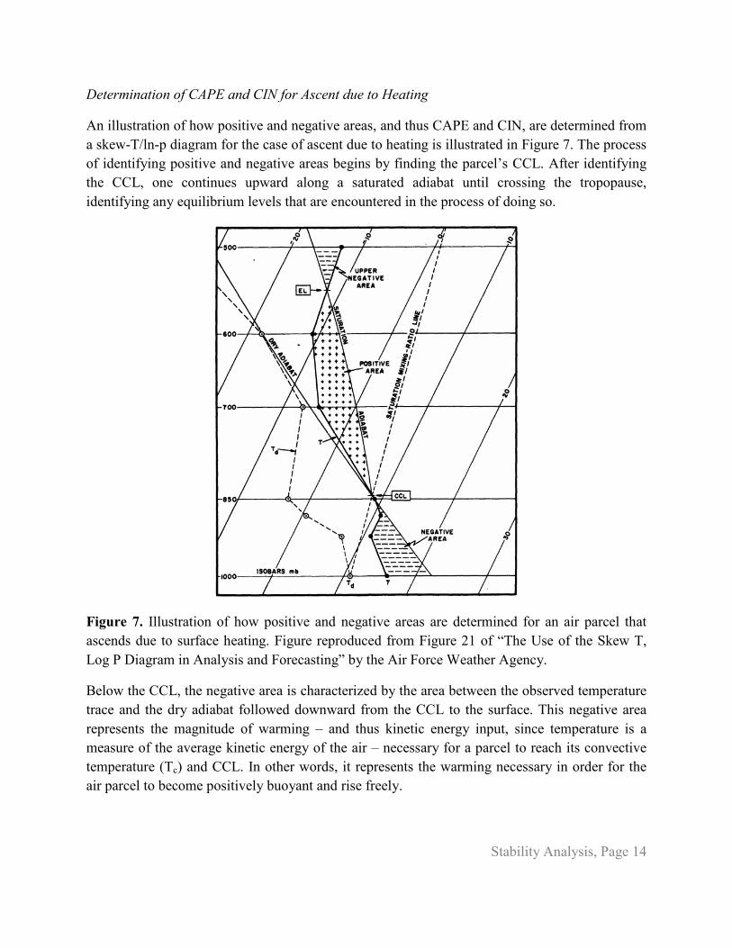
An illustration of how positive and negative areas, and thus CAPE and CIN, are determined from a skew-T/ln-p diagram for the case of ascent due to heating is illustrated in Figure 7. The process of identifying positive and negative areas begins by finding the parcel’s CCL. After identifying the CCL, one continues upward along a saturated adiabat until crossing the tropopause, identifying any equilibrium levels that are encountered in the process of doing so.

Figure 7. Illustration of how positive and negative areas are determined for an air parcel that ascends due to surface heating. Figure reproduced from Figure 21 of “The Use of the Skew T, Log P Diagram in Analysis and Forecasting” by the Air Force Weather Agency.

Below the CCL, the negative area is characterized by the area between the observed temperature trace and the dry adiabat followed downward from the CCL to the surface. This negative area represents the magnitude of warming – and thus kinetic energy input, since temperature is a measure of the average kinetic energy of the air – necessary for a parcel to reach its convective temperature (Tc) and CCL. In other words, it represents the warming necessary in order for the air parcel to become positively buoyant and rise freely.

Stability Analysis,

Above the CCL, we first encounter a positive area. Positive area(s) represent the situation where the ascending parcel trace is found to the right of the observed temperature trace, such that the ascending parcel is warmer (less dense) than its surroundings. Greater separation between these two traces results in a larger positive area and, thus, greater CAPE. In the example in Figure 7, we subsequently encounter another negative area. Negative area(s) above the CCL represent the situation where the ascending parcel trace is found to the left of the observed temperature trace, such that the ascending parcel is cooler (more dense) than its surroundings. Greater separation between these two traces results in a larger negative area and, thus, greater CIN.

Consider the case of Figure 7. The negative area between the surface and the CCL represents the CIN that must be overcome – by surface heating in this case – in order for an air parcel to reach its CCL. The positive area between the CCL and the EL represents the CAPE available to this air parcel. The EL at approximately 550 hPa represents an upper bound on the air parcel’s ascent and the negative area above the EL represents CIN that must be overcome by some means in order for an air parcel to be able to ascend above 550 hPa.

Determination of CAPE and CIN for Ascent due to Forced Lifting

An illustration of how positive and negative areas, and thus CAPE and CIN, are determined from a skew-T/ln-p diagram for the case of ascent due to forced lifting is illustrated in Figure 8. The process of identifying positive and negative areas begins by finding the parcel’s LCL. After identifying the LCL, one continues upward along a saturated adiabat until crossing the tropopause, identifying the LFC (if present) and any equilibrium levels that are encountered in the process of doing so.

Whether above or below the LFC, negative areas represent the situation where the ascending parcel trace is found to the left of the observed temperature trace, such that the air parcel is colder and more dense than its surroundings. Positive areas represent the situation where the ascending parcel trace is found to the right of the observed temperature trace, such that the air parcel is warmer and less dense than its surroundings. The lower negative area in Figure 8 represents the CIN that must be overcome in order for a parcel to reach its LFC; the upper negative area represents the CIN that must be overcome in order for a parcel to be able to rise beyond its EL. The positive area represents the CAPE available to the ascending air parcel.

Stability Analysis,

Figure 8. Illustration of how positive and negative areas are determined for an air parcel that ascends due to forced lifting. Figure reproduced from Figure 22 of “The Use of the Skew T, Log P Diagram in Analysis and Forecasting” by the Air Force Weather Agency.

Graphical Estimation of CAPE and CIN

On the skew-T/ln-p diagrams available from the course website, skewed isotherms are drawn at 1°C intervals and dry adiabats are drawn at 2°C intervals. The area of the rectangle cut out between two adjacent isotherms and two adjacent dry adiabats represents approximately 7 J kg-1 of energy, whether in terms of CIN or CAPE. Thus, summing up the number of filled and partially-filled rectangles within positive and negative areas and multiplying by this 7 J kg-1 value enables us to graphically estimate the CAPE and CIN present for a given scenario.

How is CIN Overcome to Unlock CAPE?

The observed sounding in Figure 8 is identical to that in Figure 7. This allows us to clearly illustrate that the positive and negative areas – and thus CAPE and CIN – differ depending upon the means by which an air parcel initially ascends. In the real atmosphere, forced lifting generally dominates over heating, but both are generally present (or at least possible).

Stability Analysis,

For instance, consider the case of warm season thunderstorm formation over the Great Plains. Thunderstorms typically initiate during the late afternoon hours, when a surface or near-surface air parcel is closest to its convective temperature. This minimizes the lower negative areas found in both Figure 7, by bringing the observed temperature trace closer to the dry adiabat followed to find the convective temperature, and Figure 8, by causing a dry adiabat closer to the observed temperature trace to be followed to find the air parcel’s LCL.

Concurrently, one or more forced lifting mechanisms, such as associated with a frontal boundary, dry line, topographic feature, and so on, act to continually lift parcels found within the planetary boundary layer (e.g., at and beneath the inversion seen in Figures 7 and 8). Recall from before that the dry adiabatic lifting of a layer with a lapse rate that is less than the dry adiabatic lapse rate causes it to become less stable. Consequently, persistent lifting at and beneath the inversion acts to lift and weaken the inversion, thereby reducing the amount of CIN that must be overcome in order for an ascending air parcel to rise freely!

For Further Reading

Most information contained within these lecture notes is drawn from Chapters 4 and 5 of “The Use of the Skew T, Log P Diagram in Analysis and Forecasting” by the Air Force Weather Agency, a PDF copy of which is available from the course website. Chapter 5 of Weather Analysis by D. Djurić provides further details about how stability may be assessed utilizing skew-T/ln-p diagrams.

synoptic meteorology i: stability analysis why do...

Documents