synoptic meteorology i: meteorological data and an...

Meteorological Data and an Introduction to Synoptic Analysis,

Synoptic Meteorology I: Meteorological Data and an Introduction to Synoptic Analysis

2, 4 September 2014

Types of Meteorological Observations

There exist three primary types of meteorological observations:

• Visual, or observations made by the eyes of human observers. • Direct, or observations made by instruments located where the observation is taken. • Indirect, or observations of atmospheric properties at one location made by an

instrument situated at another location.

Indirect, or remotely sensed, observations can be further broken down into actively and passively sensed observations. Active sensing occurs when the observing instrument emits a signal (e.g., a radio wave or radiation) and derives meteorological information from the echo that it receives in return. Passive sensing occurs when the observing instrument does not send out a signal; instead, meteorological information is derived from an echo that the instrument receives from another emitter (e.g., the Earth).

Surface Observations

A number of surface, or near-surface, meteorological properties are routinely observed. The most important properties that are observed include:

• Surface pressure. Measured by barometers and then converted to sea level pressure by adding the pressure of the air between the surface and sea level to the surface pressure.

• Surface temperature. Measured by thermometers located about 1.5-2 m above ground in white-painted shelters, with the shelter typically sited in an open, grass-covered field.

• Wind speed and direction. Measured by anemometers and wind vanes, respectively, located 10 m above ground, above most ground-based obstructions.

• Moisture. Dew point is measured by measuring changes in laser beam reflection off of a mirror that occur when the mirror is cooled to the dew point.

• Precipitation. Rain and the liquid equivalent of frozen precipitation are measured using a heated tipping bucket rain gauge. Snowfall is measured on white-painted snow boards.

• Visibility. Visibility is typically estimated using active remote sensing, though such estimates can be augmented by visual observation by human observers.

• Cloud type, altitude, and coverage. Cloud type and coverage are determined visually by human observers. The altitude of cloud bases is determined by active remote sensing.

• Meteorological phenomena. The presence of sensible weather, such as precipitation type, precipitation intensity, and the like, is assessed by human observers.


Other meteorological properties, such as pressure tendency and relative humidity, can be derived from one or more of the above properties. Most surface observations are collected by automated surface weather stations. The most common such station is known as ASOS, or Automated Surface Observing System. Other such stations include AWOS (Automated Weather Observing System) and AWSS (Automated Weather Sensor System). ASOS stations are typically better-calibrated, better-maintained, and more accurate than their AWOS and AWSS counterparts.

Surface observations are typically collected at regular intervals of as frequent as every 1-2 min. However, surface observations are only routinely transmitted every 1 h unless the local weather conditions are rapidly changing (e.g., a thunderstorm, cold frontal passage, or onset/termination of precipitation). In such cases, surface observations are transmitted as often as the weather conditions warrant.

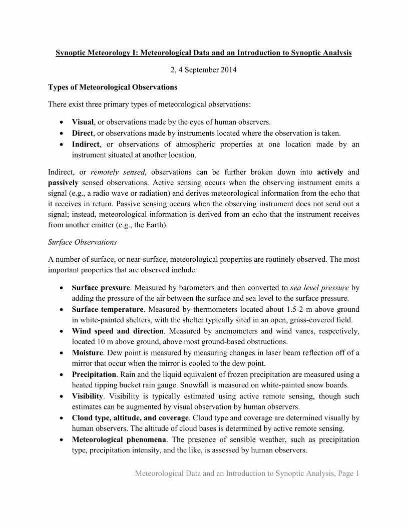
Surface observations are collected over an irregularly-spaced network of stations, with stations typically sited at airports. The average spacing between stations can and often does vary within a state, between states, and between countries. This spacing tends to be smaller in developed countries, particularly in the middle latitudes, and larger over water, near the poles, and in developing countries. Figure 1 below depicts the Federal Aviation Administration network of surface observing stations in Wisconsin.

Figure 1. Locations of Federal Aviation Administration surface weather observation stations in Wisconsin, current as of summer 2014. The different colored pins denote differences in the instruments installed at each station, with grey pins denoting ASOS stations. Note the lesser density of stations in west-central and northern Wisconsin as compared to southern and eastern Wisconsin. Image obtained from the Federal Aviation Administration.


Upper Air Observations

Similar to surface observations, a number of meteorological properties above the surface are routinely and directly observed. These observations are known as upper air observations, referring to their location above the surface. Most such observations are found within the troposphere, or below about 15 km above sea level, and are collected utilizing radiosondes, rawinsondes, dropsondes, or by aircraft utilizing an instrument package known as ACARS.

Of these, rawinsondes are the most commonly encountered observation platform. Rawinsondes are meteorological instrument packages tethered to balloons that measure meteorological properties such as pressure, temperature, relative humidity, and wind speed and direction. Other properties, such as geopotential height, can be derived from these fields. Rawinsondes are released from surface-based observing stations and relay upper air meteorological data back to the surface using radio transmitters.

Radiosondes are similar to rawinsondes, except lacking the ability to measure wind speed and direction. Dropsondes are also similar to rawinsondes, except they are released from airbone platforms, are attached to a parachute rather than a balloon, and fall to the ground rather than rise away from it. By contrast, ACARS are fixed to an aircraft and transmit data to the ground via satellite. They are particularly useful for measuring atmospheric properties over open waters.

Upper air data are reported on a set of mandatory (or standard) isobaric surfaces as well as at pressure levels where a significant change occurs in the observed temperature, relative humidity, or wind profiles. The mandatory isobaric surfaces on which upper air observations are reported are 1000, 925, 850, 700, 500, 400, 300, 250, 200, 150, 100, 70, 50, 30, 20, and 10 hPa. Observations terminate at the altitude at which the balloon carrying the instrument package pops.

In contrast to surface observations, upper air observations are routinely taken only every 12 h at times coordinated across the globe, 0000 UTC and 1200 UTC, where UTC refers to Universal Coordinated Time. These times correspond to midnight and noon, respectively, along the Prime Meridian (0° longitude), and equate to 6 pm CST/7 pm CDT and 6 am CST/7 am CDT, respectively. Some stations, particularly in developing countries, only take observations once daily at 0000 UTC, while high-impact weather conditions such as severe weather or hurricanes occasionally warrant collecting upper air observations more frequently (e.g., every 6 h).

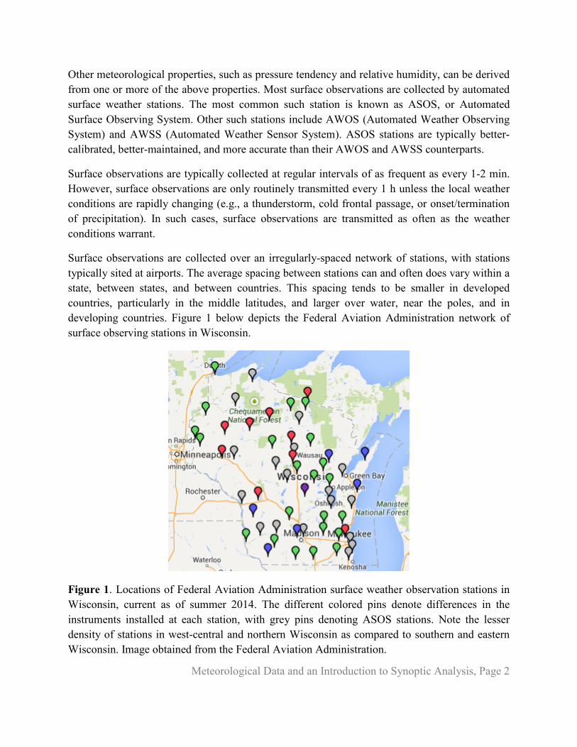
While upper air observations are also taken over an irregularly-spaced network of stations, their density is even less than that of surface stations. The average spacing between upper air observing stations in the United States is approximately 315 km. Figure 2 below depicts the locations of upper air observation stations across the United States and adjacent locales.


Figure 2. Locations of upper air observation stations across the United States and portions of Canada, Mexico, and the western Caribbean Sea, current as of summer 2014. Note the rather large spacing between stations in Canada as compared to the United States and Mexico. Image obtained from the National Center for Atmospheric Research.

Remotely Sensed Observations

There exist many platforms by which remotely sensed observations are routinely obtained. Examples include profilers, lidars, lightning arrays, and scatterometers. However, the two most common remote sensing platforms are radars (specifically, Doppler radars) and satellite imagers.

Doppler radars enable us to determine precipitation location, intensity, and type; infer wind speed and direction (with respect to the radar); and analyze the four-dimensional structure of precipitating meteorological phenomena. Doppler radars are active remote sensors; they send out radio waves and sense what is returned to the radar by both meteorological and non-meteorological phenomena. Radio waves are sent out by a Doppler radar approximately every five minutes at multiple elevation angles above the horizon, typically between 0.5° and 19°. The functional viewable range of a Doppler radar is between 100 km and 200 km from the radar, and there are presently 155 Doppler radar sites located across the United States and its territories.

Precipitation intensity can be inferred by the amount of wave energy returned to the Doppler radar; more energy implies heavier precipitation. Precipitation location can be inferred by the amount of time it takes for the wave energy to be returned to the radar as well as from which direction it is returned to the radar. Precipitation type can be inferred utilizing what is known as dual polarization radar. Wind speed and direction (with respect to the radar) can be inferred using the Doppler effect, where the change in frequency of the radio waves sent out versus returned to the radar enables for these properties to be inferred.


Satellite imagers are passive remote sensors; they measure radiation energy emitted and/or reflected by the Earth and its atmosphere at specific wavelengths. This information can then be converted into usable meteorological information, particularly as it relates to the presence, thickness, and altitude of clouds. There exist multiple types of satellite imagers, with the three most prevalent being visible, infrared, and water vapor imagers. We will discuss each in more detail shortly.

There exist two types of satellites that are used for meteorological observation:

• Geostationary. These satellites are located approximately 36,000 km above the Earth’s surface. They remain in a fixed location, above the Equator and at a specific longitude, and provide satellite imagery primarily over the tropics and middle latitudes. Imagery are available every 30 min to 3 h for any given location.

• Polar orbiting. These satellites rotate around the Earth at altitudes of 700 to 1,000 km above the Earth’s surface. A polar orbiting satellite thus passes over a given location only twice per day. Polar orbiting satellites provide imagery at all latitudes, often with a higher spatial resolution than geostationary satellites.

As noted above, there are three primary types of satellite imagers, each of which senses radiation emitted and/or reflected by the Earth and its atmosphere over a specific wavelength band. For the visible imager, this is between 0.52 μm and 0.72 μm, or within the visible light spectrum. For the infrared imager, this is between 10.2 μm and 11.2 μm, or within what is known as the “atmospheric window.” Finally, for the water vapor infrared imager, this is between 6.47 μm and 7.02 μm, within the infrared portion of the spectrum.

Visible satellite imagery is derived from the amount of sunlight that is reflected by the Earth, whether by clouds or the Earth’s surface, back to outer space. As a result, visible satellite imagery is only available during the local daytime hours. Visible satellite imagery is good for distinguishing the amount of water or ice present within a cloud. Whiter, brighter colors denote clouds with greater amounts of water or ice. Dark colors typically denote the Earth’s surface.

Infrared satellite imagery is derived from the amount of radiation emitted by the Earth, whether by clouds or by the Earth’s surface, to outer space within the atmospheric window. Through the Stefan-Boltzmann Law, the measured amount of emitted radiation can be used to estimate the temperature of the phenomenon that is emitting the radiation. Since temperature typically decreases with increasing height above sea level within the troposphere, this allows us to estimate cloud height at a given location. Colder temperatures correspond to higher cloud tops.

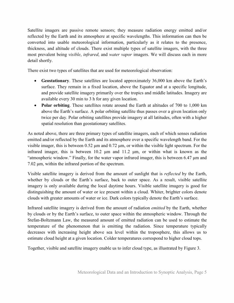
Together, visible and satellite imagery enable us to infer cloud type, as illustrated by Figure 3.


Figure 3. Illustration of cloud type inferences based upon a cloud’s appearance in visible and infrared satellite imagery. Figure obtained from Meteorology: Understanding the Atmosphere (4th Ed.) by S. Ackerman and J. Knox, their Figure 5-16.

Water vapor satellite imagery is derived from the emission of radiation by water vapor molecules present within the middle to upper troposphere. It is obtained at a wavelength of roughly 6.47 μm to 7.02 μm, as this is the wavelength band in which the peak emission of radiation by water vapor is found. Areas of clouds and greater moisture content, even if cloud-free, appear brighter in water vapor satellite imagery, whereas drier areas appear in darker colors. Water vapor satellite imagery is useful for diagnosing moist processes in the middle to upper troposphere that are important to cyclone formation and intensification.

Representativeness of Observations

All instruments are associated with some amount of observational error, even if the instrument is in good working order. Typical magnitudes of observational error are 0.5 to 1 m s-1 for wind speed, 0.25°C for temperature, 3% for relative humidity, 0.5 hPa for pressure, and 5 m for geopotential height for both surface and upper air observations. Indirect observation instruments such as radars and satellites are also associated with observational error, the magnitudes of which vary between individual instruments. It should be noted that observational errors are typically small compared to the magnitudes of the observed meteorological elements and, as a result, observational error typically does not compromise our ability to analyze and interpret data.

There exist situations, however, where one or more observations, whether taken at the surface or aloft, are not representative of the prevailing meteorological conditions at that location. Plausible reasons for why this might be the case for include:


• Improper siting of the observation instrument (e.g., a bank thermometer). • The observation instrument has failed and/or has lost its proper calibration. • The observation collected is correct but is representative of local rather than synoptic-

scale meteorological conditions and variability.

We must take care to properly identify and discard observations that fit into the first or second of the above criteria. We must also take care to properly identify but not discard observations that fit into the third of the above criteria. How can we do this? We can do so by considering how observations at that station compare to those at surrounding stations at other times.

We can also do so by considering how observations at that station align with theory. In other words, based upon our knowledge of how the atmosphere works (e.g., force balances, structures of specific meteorological phenomena, local climatology, etc.), is the observation likely to be correct or in error? Over the course of this semester, we seek to develop your knowledge of meteorological theory so that you will be well-equipped to judge an observation’s representativeness. When in doubt, however, we must always assume that the observation is correct; we cannot simply discount an observation that we don’t like without good reasoning.

Surface Observations: The METAR Code

The United States standard means of encoding and reporting surface weather conditions at a given location and time is known as the aviation routine weather report, or METAR, code. Weather observations that you see on television, on weather charts, hear pilots mention while flying, and elsewhere are all derived by interpreting METAR code. Below, a generic example METAR observation is provided:

METAR CCCC DDGGggZ AUTO/COR dddffGggKT vvSM ww NNNhhh TT/DD Apppp RMK (remarks)

Working from left to right, the METAR provides the following surface weather information:

• METAR. This identifies the text as a METAR observation. • CCCC. This is replaced by a unique four-letter identifier that denotes the location of the

observation. In the United States, the first letter is K. For example, the observation station at General Mitchell Airport here in Milwaukee is KMKE.

• DDGGggZ. This denotes the time of the observation. DD is replaced by the two-digit date of the month, while GGgg is replaced by the four-digit time. The Z denotes Zulu time, which is equivalent to UTC, and thus observations are not reported in local time.

• AUTO/COR. This denotes whether the observation is an automated (AUTO) or manually-corrected (COR) observation.

• dddffGggKT. This indicates the wind direction (ddd, where 000 = from the north, 090 = from the east, 180 = from the south, and 270 = from the west), wind speed (ff), and, if


present, wind gust (Ggg, where gg is the gust speed). The ending KT denotes that the wind and gust speed are in kt.

• vvSM. This indicates the current surface visibility (vv) in units of statute miles (SM). The maximum reported visibility is typically 10SM.

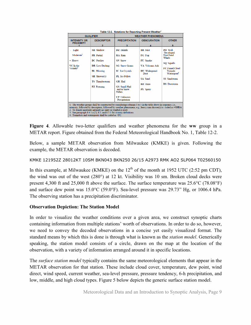
• ww. This denotes the sensible weather present at a given location, if any. There exist a series of two-letter qualifiers for intensity, proximity, and/or description. These are followed by one or more two-letter identifiers for current weather phenomena, classified under precipitation, obscuration, or other. Figure 4 below provides a full listing.

• NNNhhh. This denotes cloud coverage (NNN, which could be CLR, FEW, SCT, BKN, or OVC depending upon coverage) and height (hhh, in hundreds of feet above the surface). Overcast skies 10,000 feet above the surface would be coded as OVC100.

• TT/DD. This indicates the two-digit surface temperature (TT) and dew point (DD), separated by a /, with both values in °C.

• Apppp. This indicates the current altimeter (A), or sea-level pressure, reading (pppp, in inches of mercury multiplied by 100). A sea-level pressure of 29.92” Hg would be encoded as A2992.

• RMK (remarks). A series of remarks, whether automated or manual, plain-language or encoded, is often appended to the end of a METAR statement. The most common are as follows:

o A01/A02. Denotes whether the observing station has a precipitation discriminator (A02) or not (A01).

o SLP###. Indicates the sea-level pressure (SLP) reading in hPa multiplied by 10. For sea-level pressure less than 1000 hPa, the leading 9 is dropped; for sea-level pressure greater than or equal to 1000 hPa, the leading 10 is dropped. A sea-level pressure of 1013.2 hPa would be reported as SLP132.

o Tttttdddd. Denotes the surface temperature and dew point, both in °C, multiplied by 10. The first ‘t’ and ‘d’ in each sequence are replaced by 0 if the reading is above 0°C and replaced by 1 if the reading is below 0°C. A temperature of 24.2°C and dew point of 18.1°C would be encoded as T02420181.

There exist many other remarks, and not every possible element of a METAR statement is listed above. Chapter 12 of the Federal Meteorological Handbook No. 1 provides full details regarding all possible elements of a METAR statement. Real-time METAR observations, including a list of possible stations, may be obtained from the National Center for Atmospheric Research’s Real-Time Weather Data page at http://weather.rap.ucar.edu/surface/.

http://weather.rap.ucar.edu/surface/


Figure 4. Allowable two-letter qualifiers and weather phenomena for the ww group in a METAR report. Figure obtained from the Federal Meteorological Handbook No. 1, Table 12-2.

Below, a sample METAR observation from Milwaukee (KMKE) is given. Following the example, the METAR observation is decoded.

KMKE 121952Z 28012KT 10SM BKN043 BKN250 26/15 A2973 RMK AO2 SLP064 T02560150

In this example, at Milwaukee (KMKE) on the 12th of the month at 1952 UTC (2:52 pm CDT), the wind was out of the west (280°) at 12 kt. Visibility was 10 sm. Broken cloud decks were present 4,300 ft and 25,000 ft above the surface. The surface temperature was 25.6°C (78.08°F) and surface dew point was 15.0°C (59.0°F). Sea-level pressure was 29.73” Hg, or 1006.4 hPa. The observing station has a precipitation discriminator.

Observation Depiction: The Station Model

In order to visualize the weather conditions over a given area, we construct synoptic charts containing information from multiple stations’ worth of observations. In order to do so, however, we need to convey the decoded observations in a concise yet easily visualized format. The standard means by which this is done is through what is known as the station model. Generically speaking, the station model consists of a circle, drawn on the map at the location of the observation, with a variety of information arranged around it in specific locations.

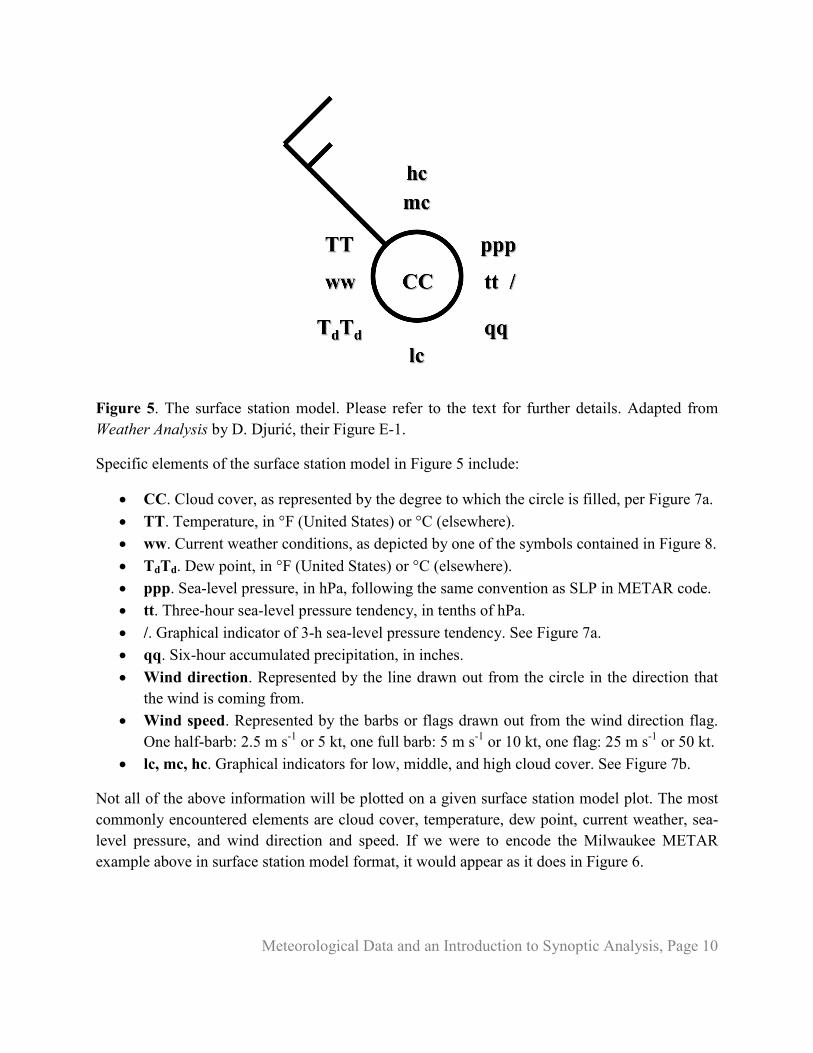
The surface station model typically contains the same meteorological elements that appear in the METAR observation for that station. These include cloud cover, temperature, dew point, wind direct, wind speed, current weather, sea-level pressure, pressure tendency, 6-h precipitation, and low, middle, and high cloud types. Figure 5 below depicts the generic surface station model.


Figure 5. The surface station model. Please refer to the text for further details. Adapted from Weather Analysis by D. Djurić, their Figure E-1.

Specific elements of the surface station model in Figure 5 include:

• CC. Cloud cover, as represented by the degree to which the circle is filled, per Figure 7a. • TT. Temperature, in °F (United States) or °C (elsewhere). • ww. Current weather conditions, as depicted by one of the symbols contained in Figure 8. • TdTd. Dew point, in °F (United States) or °C (elsewhere). • ppp. Sea-level pressure, in hPa, following the same convention as SLP in METAR code. • tt. Three-hour sea-level pressure tendency, in tenths of hPa. • /. Graphical indicator of 3-h sea-level pressure tendency. See Figure 7a. • qq. Six-hour accumulated precipitation, in inches. • Wind direction. Represented by the line drawn out from the circle in the direction that

the wind is coming from. • Wind speed. Represented by the barbs or flags drawn out from the wind direction flag.

One half-barb: 2.5 m s-1 or 5 kt, one full barb: 5 m s-1 or 10 kt, one flag: 25 m s-1 or 50 kt. • lc, mc, hc. Graphical indicators for low, middle, and high cloud cover. See Figure 7b.

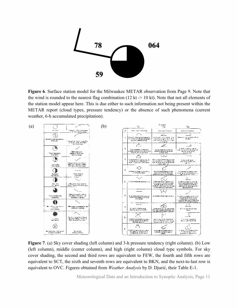
Not all of the above information will be plotted on a given surface station model plot. The most commonly encountered elements are cloud cover, temperature, dew point, current weather, sea-level pressure, and wind direction and speed. If we were to encode the Milwaukee METAR example above in surface station model format, it would appear as it does in Figure 6.


Figure 6. Surface station model for the Milwaukee METAR observation from Page 9. Note that the wind is rounded to the nearest flag combination (12 kt -> 10 kt). Note that not all elements of the station model appear here. This is due either to such information not being present within the METAR report (cloud types, pressure tendency) or the absence of such phenomena (current weather, 6-h accumulated precipitation).

(a)

(b)

Figure 7. (a) Sky cover shading (left column) and 3-h pressure tendency (right column). (b) Low (left column), middle (center column), and high (right column) cloud type symbols. For sky cover shading, the second and third rows are equivalent to FEW, the fourth and fifth rows are equivalent to SCT, the sixth and seventh rows are equivalent to BKN, and the next-to-last row is equivalent to OVC. Figures obtained from Weather Analysis by D. Djurić, their Table E-1.


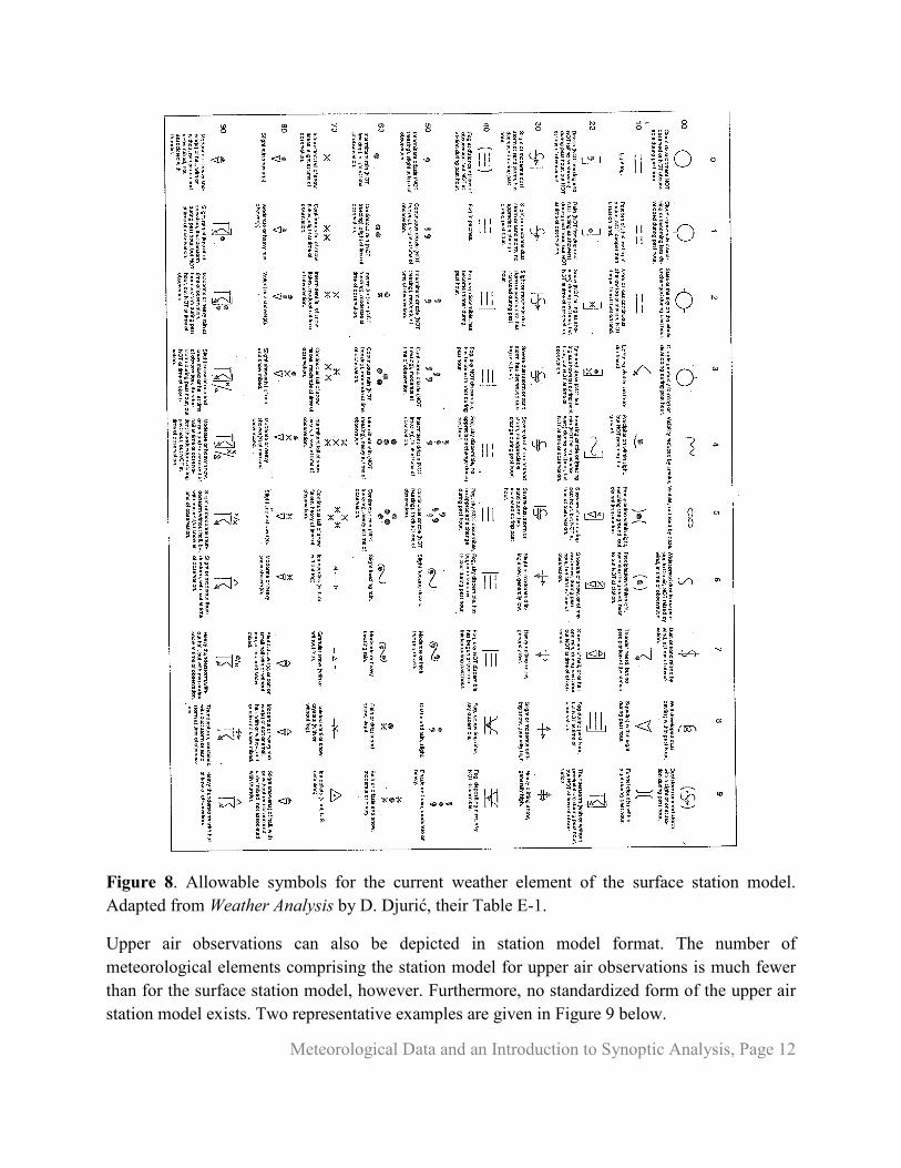
Figure 8. Allowable symbols for the current weather element of the surface station model. Adapted from Weather Analysis by D. Djurić, their Table E-1.

Upper air observations can also be depicted in station model format. The number of meteorological elements comprising the station model for upper air observations is much fewer than for the surface station model, however. Furthermore, no standardized form of the upper air station model exists. Two representative examples are given in Figure 9 below.


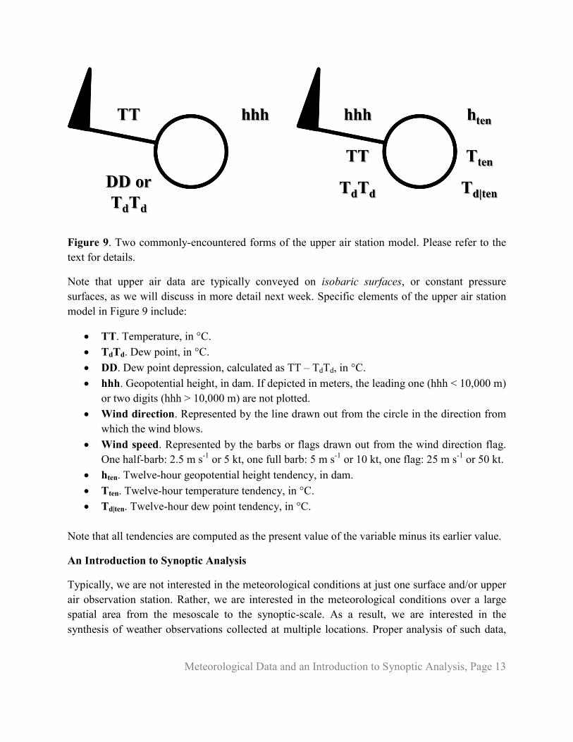
Figure 9. Two commonly-encountered forms of the upper air station model. Please refer to the text for details.

Note that upper air data are typically conveyed on isobaric surfaces, or constant pressure surfaces, as we will discuss in more detail next week. Specific elements of the upper air station model in Figure 9 include:

• TT. Temperature, in °C. • TdTd. Dew point, in °C. • DD. Dew point depression, calculated as TT – TdTd, in °C. • hhh. Geopotential height, in dam. If depicted in meters, the leading one (hhh < 10,000 m)

or two digits (hhh > 10,000 m) are not plotted. • Wind direction. Represented by the line drawn out from the circle in the direction from

which the wind blows. • Wind speed. Represented by the barbs or flags drawn out from the wind direction flag.

One half-barb: 2.5 m s-1 or 5 kt, one full barb: 5 m s-1 or 10 kt, one flag: 25 m s-1 or 50 kt. • hten. Twelve-hour geopotential height tendency, in dam. • Tten. Twelve-hour temperature tendency, in °C. • Td|ten. Twelve-hour dew point tendency, in °C.

Note that all tendencies are computed as the present value of the variable minus its earlier value.

An Introduction to Synoptic Analysis

Typically, we are not interested in the meteorological conditions at just one surface and/or upper air observation station. Rather, we are interested in the meteorological conditions over a large spatial area from the mesoscale to the synoptic-scale. As a result, we are interested in the synthesis of weather observations collected at multiple locations. Proper analysis of such data,


both at the surface and aloft, enables meteorologists to identify the four-dimensional location, structure, and evolution of meteorological phenomena such as fronts and air masses.

For this analysis, we employ a technique known as isoplething to the data. Isopleths connect points on a map that have the same value of whatever quantity is being examined. Commonly isoplethed meteorological elements include temperature, potential temperature, dew point, sea-level pressure, pressure tendency, wind speed, geopotential height, and geopotential height tendency. Isopleths of these quantities are known as isotherms, isentropes, isodrosotherms, isobars, isallobars, isotachs, isohypses, and isallohypses, respectively.

As we discussed earlier in this lecture, meteorological observations are discrete; we do not have data at every possible location. Thus, isoplething involves interpolation of the values of the quantity being examined between the observations. To do so, we assume that meteorological fields are continuous; i.e., if the temperature is 10°C at one point and 20°C at the nearest adjacent point, we assume that the temperature between the two points changes smoothly and uniformly between the two points.

You will often encounter features in isoplethed analyses – particularly of sea-level pressure and geopotential height – that have specific names. These include:

• Low. A local minimum in the field, often depicted by at least one closed isopleth. • High. A local maximum in the field, often depicted by at least one closed isopleth. • Trough line. A dashed line connecting points of maximum isopleth curvature, where the

isopleths bend or curve around lower values of the isoplethed field. • Ridge line. A jagged line connecting points of maximum isopleth curvature, where the

isopleths bend or curve around higher values of the isoplethed field. • Trough. The region around a trough line. • Ridge. The region around a ridge line. • Col. The hyperbolic point between a pair of ridges and a pair of troughs. • Wave. A combination of a single trough and a single ridge.

When preparing an isoplethed analysis, there are a number of guidelines that should be followed. The most important of these guidelines is that isopleths should satisfy the conceptual model of the atmosphere most applicable to the isoplethed field. Examples of such conceptual models include frontal structure, geostrophic balance, and vertical structure. Our analysis should also be consistent with that at an earlier time, if such an analysis is available. We will introduce several conceptual models applicable to synoptic-scale phenomena throughout the course of this semester, and we will examine isoplething techniques for the relevant field(s) at those times.

Other guidelines that should be followed include the following:


1. Pick an appropriate interval for the isopleths. Commonly encountered values include 4 hPa for sea-level pressure, 30 m or 60 m for geopotential height, 10 kt to 20 kt for wind speed, and 2°C to 5°C for temperature and dew point. This interval should be evenly divisible into the values of your isopleths.

2. Since meteorological fields are assumed to be continuous, isopleths should not start or stop in the middle of a field; there should not be breaks in the isopleths; isopleths do not branch from or merge into each other; and isopleths do not intersect. Thus, isopleths are either closed or extend from one edge of the data to the other.

3. Isopleths should only reflect the level of detail allowed by the available data. Do not make up data simply because you think the isopleths should look a specific way.

4. Isopleths should be evenly spaced unless there is a specific reason for their spacing to vary, such as tied to a conceptual model of the atmosphere.

5. Terminate isopleths shortly after the data stop, such as along coastlines.

6. Assume that each observation is correct unless you can prove beyond a reasonable doubt that it is in error, following the guidelines under “Representativeness of Observations” above. Circle any observations that you do exclude from your analysis.

7. Your isopleth analysis should be neat, including isopleths that are both smooth and labeled at their ends. Erase all errors or preliminary markings.

8. For closed isopleths, place a “H” (for maxima) or “L” (for minima) at the center and interpolate the central value, writing it neatly in a horizontal fashion under the letter.

9. Begin by surveying the data in its entirety. Start your actual analysis in “easy” locations, where the isopleth pattern is obvious, and proceed outward from there. Ensure that the above guidelines are met as you conduct and finalize your analysis.

For Further Reading

Chapter 12 of Midlatitude Synoptic Meteorology by G. Lackmann discusses principles of isoplething and meteorological data analysis. Chapter 2, Sections 3-2 and 3-3, and Appendix E of Weather Analysis by D. Djurić provide useful information regarding observations, synoptic analysis, and surface meteorological data encoding and decoding, respectively. Federal Meteorological Handbook No. 1 provides extensive information concerning how surface meteorological observations are obtained and encoded. Federal Meteorological Handbook No. 2 provides extensive information concerning the international-standard SYNOP surface observation encoding protocol. Federal Meteorological Handbook No. 3 provides extensive information concerning how upper air meteorological observations are obtained and encoded.

synoptic meteorology i: meteorological data and an...

Documents