Surface Approximation and Geometric Partitions �Pankaj K. AgarwalDepartment of Computer ScienceBox 1029, Duke UniversityDurahm, NC 27708-0129. Subhash SuriBell Communications Research445 South StreetMorristown, NJ 07960.February 19, 1996AbstractMotivated by applications in computer graphics, visualization, and scienti�c com-putation, we study the computational complexity of the following problem: Given aset S of n points sampled from a bivariate function f(x; y) and an input parameter" > 0, compute a piecewise-linear function �(x; y) of minimum complexity (that is, axy-monotone polyhedral surface, with a minimum number of vertices, edges, or faces)such that j�(xp; yp) � zpj � "; for all (xp; yp; zp) 2 S:We prove that the decision version of this problem is NP-Hard . The main result of ourpaper is a polynomial-time approximation algorithm that computes a piecewise-linearsurface of size O(Ko logKo), whereKo is the complexity of an optimal surface satisfyingthe constraints of the problem.The technique developed in our paper is more general and applies to several otherproblems that deal with partitioning of points (or other objects) subject to certaingeometric constraints. For instance, we get the same approximation bound for thefollowing problem arising in machine learning: given n `red' and m `blue' points in theplane, �nd a minimum number of pairwise disjoint triangles such that each blue pointis covered by some triangle and no red point lies in any of the triangles.1 IntroductionIn scienti�c computation, visualization, and computer graphics, the modeling and construc-tion of surfaces is an important area. A small sample of some recent papers [1, 2, 4, 8, 11,14, 22, 23] on this topic gives an indication of the scope and importance of this problem.�The �rst author has been supported by National Science Foundation Grant CCR{93{01259 and an NYIaward. 1

Introduction 2Rather than delve into any speci�c problem studied in these papers, we focus on a general,abstract problem that seems to underlie them all.In many scienti�c and computer graphics applications, computation takes place overa surface in three dimensions. The surface is generally modeled by piecewise linear (or,sometimes piecewise cubic) patches, whose vertices lie either on or in the close vicinity ofthe actual surface. In order to ensure that all local features of the surface are captured,algorithms for an automatic generation of these models generally sample at a dense set ofregularly spaced points. Demands for real-time speed and reasonable performance, however,require the models to have as small a combinatorial complexity as possible. A commontechnique employed to reduce the complexity of the model is to somehow \thin" the surfaceby deleting vertices with relatively \ at" neighborhoods. Only ad hoc and heuristic methodsare known for this key step. Most of the thinning methods follow a set of local rules (suchas deleting edges or vertices whose incident faces are almost coplanar), which are appliedin an arbitrary order until they are no longer applicable. Not surprisingly, these methodscome with no performance guarantee, and generally no quantitative statement can be madeabout the surface approximation computed by them.In this paper, we address the complexity issues of the surface approximation problem forsurfaces that are xy-monotone. These surfaces represent the graphs of continuous bivariatefunctions f(x; y), and they arise quite naturally in many scienti�c applications. One possibleapproach for handling arbitrary surfaces is to break them into monotone pieces, and applyour algorithm individually on each piece. Let us formally de�ne the main problem studiedin our paper.Let f be a continuous function of two variables x and y, and let S be a set of n pointssampled from f . A continuous piecewise-linear function � is called an "-approximation off , for " > 0, if j�(xp; yp)� zpj � ";for every point p = (xp; yp; zp) 2 S. Given S and ", the surface-approximation problem isto compute a piecewise-linear function � that "-approximates f with a minimum numberof breakpoints. The breakpoints of � can be arbitrary points of R3 , and they are notnecessarily points of S. In many applications, f is generally a function hypothesized to�t the observed data|the function � is a computationally e�cient substitute for f . Theparameter " is used to achieve a complexity-quality tradeo� | smaller the ", higher the�delity of the approximation. (The graph of a piecewise-linear function of two variables isalso called a polyhedral terrain in computational geometry literature; the breakpoints of thefunction are the vertices of the terrain.)Although there is a vast literature on the surface-approximation problem in graphicscommunity, the state of theoretical knowledge on this problem appears to be rather slim.The provable performance bounds are known only for convex surfaces. For this specialcase, an O(n3) time algorithm is presented by Mitchell and Suri [17] for computing anGeometric Partitioning February 19, 1996

Introduction 3"-approximation of a convex polytope of n vertices in R3 . Their algorithm produces anapproximation of size O(Ko log n), where Ko is the size of an optimal "-approximation.Extending their work, Clarkson [7] has proposed an O(Kon1+�) expected time randomizedalgorithm for computing an approximation of size O(Ko logKo), where � can be an arbitrar-ily small positive number. Recently Br�onnimann and Goodrich [5] have re�ned Clarkson'salgorithm and have given a polynomial-time algorithm for computing an approximation ofsize O(K0).In this paper, we study the approximation problem for surfaces that correspond tographs of bivariate functions. We show that it is NP-Hard to decide if a surface can be"-approximated using k vertices (or facets). The main result of our paper, however, is apolynomial-time algorithm for computing an "-approximating surface of a guaranteed qual-ity. If an optimal "-approximating surface of f has Ko vertices, then our algorithm producesa surface with O(Ko logKo) vertices. Observe that we are dealing with two approximationmeasures here: ", which measures the absolute z di�erence between f and the \simpli-�ed" surface �, and the ratio between the sizes of the optimal surface and the output ofour algorithm. For the lack of better terminology, we use the term \approximation" forboth measures. Notice though that " is an input (user-speci�ed) parameter, logKo is theapproximation guarantee provided by the analysis of our algorithm.The key to our approximation method is an algorithm for partitioning a set of pointsin the plane by pairwise disjoint triangles. This is an instance of the geometric set coverproblem, with an additional disjointness constraint on the covering objects (triangles).Observe that the disjointness condition on covering objects precludes the well-known greedymethod for set covering [12, 15]; in fact, we can show that a greedy solution has size(Ko2) in the worst-case. Let us now reformulate our surface-approximation problem as aconstrained geometric partitioning problem.Let �p denote the orthogonal projection of a point p 2 R3 onto the xy-plane z = 0. Ingeneral, for any set A � R3 , we use �A to denote the orthogonal projection of A onto thexy-plane. Then, in order to get an "-approximation of f , it su�ces to �nd a set of trianglesin 3-space such that (i) the projections of these triangles on plane z = 0 are pairwise disjointand they cover the projected set of points �S, and (ii) the vertical distance between a triangleand any point of S directly above/below it is at most ". Our polynomial-time algorithmproduces a family of O(Ko logKo) such triangles. We stitch together these triangles toproduce the desired surface �. The \stitching" process introduces at most a constant factormore triangles.The geometric partition framework also includes several extensions and generalizationsof the basic surface-approximation problem. For instance, we can formulate a strongerversion of the problem by replacing each sample point by a horizontal triangle (or, anypolygon). Speci�cally, we are given a family of horizontal triangles (or polygons) in 3-space, whose projections on the xy-plane are pairwise disjoint. We want a piecewise-linear,Geometric Partitioning February 19, 1996

A Proof of NP-Hardness 4"-approximating surface whose maximum vertical distance from any point on the trianglesis ". Our approximation algorithm works equally well for this variant of the problem|thisvariant addresses the case when some local features of the surface are known in detail;unfortunately, our method works only for horizontal features.Finally, let us mention the planar bichromatic partition problem, which is of independentinterest in the machine learning literature: Given a set R of `red' points and another setB of `blue' points in the plane, �nd a minimum number of pairwise disjoint triangles suchthat each blue point lies in a triangle and no red point lies in any of the triangles. Ouralgorithm gives a solution with O(Ko logKo) triangles. It can also be used to construct alinear decision tree of size O(Ko logKo), which is consistent with respect to R and B, whereKo is the size of an optimal linear decision tree.The running time of our algorithms, though polynomial, is quite high, and at the momenthas only theoretical value. These being some of the �rst results in this area, however, weexpect that the theoretical time complexity of these problems would improve with furtherwork. Perhaps, some of the ideas in our paper may also shed light on the theoreticalperformance of some of the \practical" algorithms that are used in the trade.2 A Proof of NP-HardnessWe show that both the planar bichromatic partition problem and the surface-approximationproblem are NP-Hard , by a reduction from the planar 3-SAT. We do not know whetherthey are in NP since the coordinates of the triangles in the solution may require very highprecision. We recall that the 3-SAT problem consists of n variables x1; : : : ; xn, and mclauses C1; : : : ; Cm, each with three literals Ci1; Ci2; Ci3, where Cij is either xk or �xk. Theproblem is to decide whether the boolean formulaF = mi=1(Ci1 _ Ci2 _Ci3)has a truth assignment. An instance of 3-SAT is called planar if its variable-clause graphis planar. In other words, F is an instance of the planar 3-SAT if the graph G(F ) = (V;E)is planar (see [13]), where V and E are de�ned as follows:V = fx1; x2; : : : ; xng;E = f(xj ; Ci) j xi or �xi appears in Cig :Theorem 2.1 The planar bichromatic-partition problem is NP-Hard.Proof: Our construction is similar to the one used by Fowler et al. [10], who prove theintractability of certain planar geometric covering problems (without the disjointness con-dition); see also [3, 9] for similar constructions. We �rst describe our construction for theGeometric Partitioning February 19, 1996

A Proof of NP-Hardness 5bichromatic partition problem. To simplify the proof, our construction allows three or morepoints to lie on a line|the construction can be modi�ed easily to remove these degeneracies.Let F be a boolean formula, and let G = (V;E) be a straight-line planar embedding ofthe graph G(F ). We construct an instance of the red-blue point partition problem whosesolution determines whether F is satis�able.We start by placing a `blue' point at each clause node Cj, 1 � j � m. Let xi be avariable node, and let ei1; ei2; : : : ; eil be the edges incident to it. In the plane embeddingof G, the edges eij form a \star" (see Figure 1 (i)). We replace this star by its Minkowskisum with a disk of radius �, for a su�ciently small � > 0. Before performing the Minkowskisum, we shrink all the edges of the star at xi by 2�, so that the \star-shaped polygons"meeting at a clause node do not overlap (see Figure 1 (ii)). Let Pi denote the star-shapedpolygon corresponding to xi. In the polygon Pi, corresponding to each edge eij, there is atube, consisting of two copies of eij , each translated by distance �, plus a circular arc sijnear the clause node Cj.We place an even number of (say 2ki) `blue' points on the boundary of Pi, as follows.We put two points aij and bij on the circular arc sij near its tip. If Cj contains the literalxi, we put six points on the straight-line portion of Pi's boundary, three each on translatedcopies of the edge eij . On each copy, we move the middle point slightly inwards so as toreplace the original edge of Pi by a path of length two. On the other hand, if Cj containsthe literal �xi, we put four points on straight-line portion of Pi's boundary, two each ontranslated copies of the edge eij . Thus, the number of blue points added for edge eij iseither six of eight. (2ki is the total number of points put along Pi.) Let B denote the setof all blue points placed in this way, and let k =Pni=1 ki.Finally, we scatter a large (but polynomially bounded) number of `red' points so that (i)any segment connecting two blue points that are not adjacent along the boundary of somePi contains a red point, and (ii) any triangle with three blue points as its vertices containsat least one red point unless the triangle is de�ned by aijbijCj for some edge eij 2 E. (SeeFigure 1 (iii).) Let R be a set of red points satisfying the above two properties.We claim that the set of blue points B can be covered by k disjoint triangles, none ofwhich contains any red point, if and only if the formula F has a truth assignment. Our proofis similar to the one in Fowler et al. [10]; we only sketch the main ideas. The red pointsact as enforcers, ensuring that only those blue points that are adjacent on the boundary ofa Pi can be covered by a single triangle. Thus, the minimum number of triangles neededto cover all the points on Pi is ki. Further, there are precisely two ways to cover thesepoints using ki triangles| in one covering, aij and bij are covered by a single triangle forthose clauses only in which xi 2 Cj, and, in the other covering, aij and bij are covered bya single triangle for those clauses only in which �xi 2 Cj; see Figure 4 (iv). We regard the�rst covering as setting xi = 1, and the second covering as setting xi = 0.Geometric Partitioning February 19, 1996

A Proof of NP-Hardness 6x2x3C1x1 x4C2

P4P1 P3C1 C2C1a11b11

P2

P1(iii)(ii)(i)

(iv)Figure 1: (i) An instance of planar 3-SAT: F = (x1 _ �x2 _ x3) ^ (x2 _ �x3 ^ x4); (ii) Corre-sponding instance of bichromatic partition, (iii) Details of P1 and C1, only some of the redpoints lying near P1 and C1 are shown, (iv) Two possible coverings of blue points on P2.Geometric Partitioning February 19, 1996

A Proof of NP-Hardness 7Suppose xi = 1. For any clause Cj that contains xi, the points aij and bij are coveredby a single triangle, and we can cover the clause point corresponding to Cj by the sametriangle. The same holds if xi = 0 and the clause Cj contains �xi. In other words, the clausepoint of Cj can be covered for free if Cj is satis�ed. Thus, the set of blue points B can becovered by k triangles if and only if the clause point for each clause Cj is covered for free,that is, the formula F has a truth assignment. This completes our proof of NP -Hardnessof the planar bichromatic partition problem. 2Remark: The preceding construction is degenerate in that most of the red points lie onsegments connecting two blue points. There are several ways to remove these collinearities;we brie y describe one of them. For each polygon Pi, replace every blue point b on Pi bytwo blue points b0; b00, placed very close to b. (We do not make copies of `clause points' Cj ,1 � j � m.) For every pair of blue points bj; bl that we did not want to cover by a singletriangle in the original construction, we place a red point in the convex hull of b0j ; b00j ; b0l; b00l .If there are 4ki blue points on the boundary of Pi, they can be covered by ki triangles, andthere are exactly two ways to cover these blue points by ki triangles, as earlier. Followinga similar, but more involved, argument, we can prove that the set of all blue points can becovered by Pni=1 ki triangles if and only if F is satis�able.Theorem 2.2 The 3-dimensional surface-approximation problem is NP-Hard.Proof: Our construction is similar in spirit to the one for the bichromatic partition problem,albeit slightly more complex in detail. We use points of three colors: red, white and black.The `white' points lie on the plane z = 0, the `black' points lie on the plane z = 2A, andthe `red' points lie between z = 0 and z = A, where A is a su�ciently large constant.To maintain a connection with the previous construction, the black and white points playthe role of blue points, while the red points play the role of enforcers as before, restrictingthe choice of \legal" triangles that can cover the black or white points. We will describethe construction in the xy-plane, which represents the orthogonal projection of the actualconstruction. The actual construction is obtained simply by vertically translating eachpoint to its correct plane, depending on its color.We start out again by putting a `black' point at each clause node Cj. Then, for eachvariable xi, we construct the \star-shaped" polygon Pi; this part is identical to the previousconstruction. We replace each of the two straight-line edges of Pi by \concave chains," bentinward, and also make a small \dent" at the tip of the circular arc sij, as shown in Figure 2.We place 12 points on each arm of Pi, alternating in color black and white, as follows. Atthe tip of the circular arc sij, we put a white point cij at the outer endpoint of the dentand a black point dij at the inner endpoint of the dent (Figure 2 (ii)). The rest of theconstruction is shown in Figure 2 (i) | we put two more points aij ; bij on the circulararc and 4 points �lij ; �lij (1 � l � 4) on each of the two concave chains. The two pointsGeometric Partitioning February 19, 1996

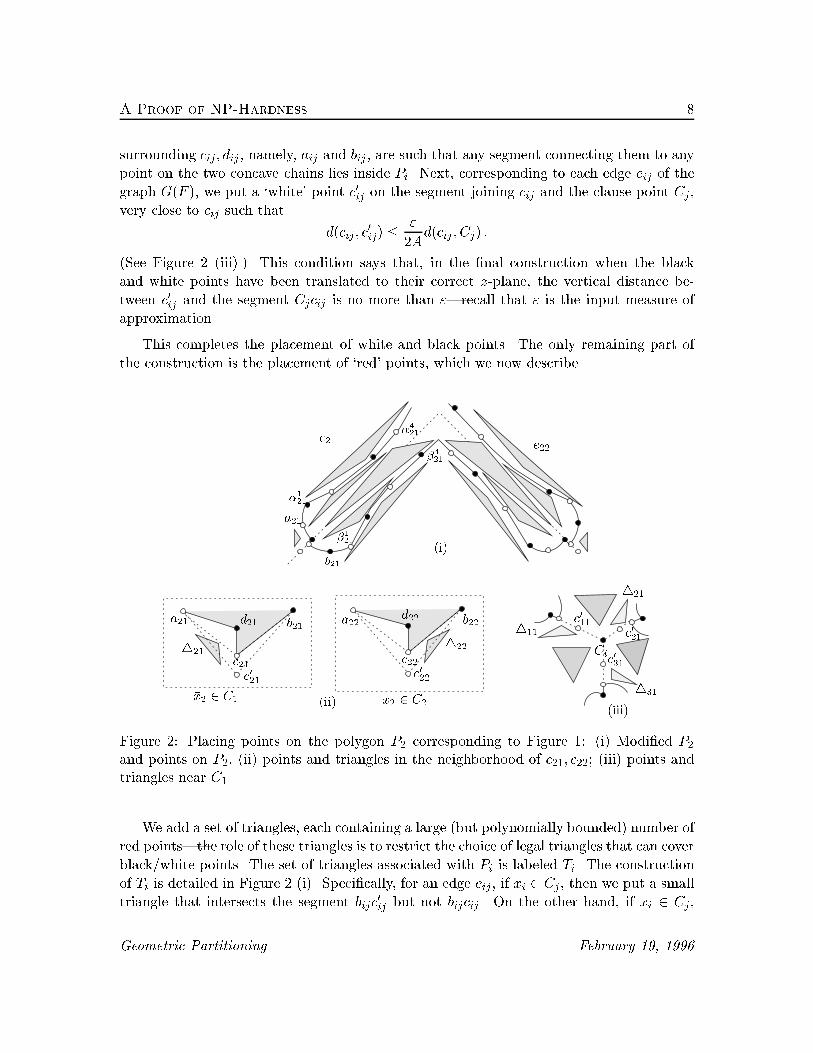
A Proof of NP-Hardness 8surrounding cij ; dij , namely, aij and bij , are such that any segment connecting them to anypoint on the two concave chains lies inside Pi. Next, corresponding to each edge eij of thegraph G(F ), we put a `white' point c0ij on the segment joining cij and the clause point Cj ,very close to cij such that d(cij ; c0ij) � "2Ad(cij ; Cj) :(See Figure 2 (iii).) This condition says that, in the �nal construction when the blackand white points have been translated to their correct z-plane, the vertical distance be-tween c0ij and the segment Cjcij is no more than "|recall that " is the input measure ofapproximation.This completes the placement of white and black points. The only remaining part ofthe construction is the placement of `red' points, which we now describe.

a22a21 b22b21d21c021 c022d22(ii) 422c22421

(i)e21 e22

c011(iii)

411 421c031b21

c21 Ci�121

�421 �421c021431�x2 2 C1 x2 2 C2

�121a21

Figure 2: Placing points on the polygon P2 corresponding to Figure 1: (i) Modi�ed P2and points on P2, (ii) points and triangles in the neighborhood of c21; c22; (iii) points andtriangles near C1.We add a set of triangles, each containing a large (but polynomially bounded) number ofred points|the role of these triangles is to restrict the choice of legal triangles that can coverblack/white points. The set of triangles associated with Pi is labeled Ti. The constructionof Ti is detailed in Figure 2 (i). Speci�cally, for an edge eij , if xi 2 Cj , then we put a smalltriangle that intersects the segment bijc0ij but not bijcij. On the other hand, if �xi 2 Cj ,Geometric Partitioning February 19, 1996

A Canonical Trapezoidal Partition 9then we put a small triangle that intersects aijc0ij but not aijcij . Next, we put a smallnumber of triangles inside Pi, near its concave chains, so that at most three consecutivepoints along Pi may be covered by one triangle without intersecting any triangle of Ti. Weensure that one of these triangles intersects the triangle 4�1ijaijdij , so that f�1ij ; aij ; dijgcannot be covered by a single triangle. We also place three triangles near each clause Cj ,each containing a large number of red points; see Figure 2 (iii). Finally, we translate blackand white points in the z-direction, as described earlier. Let f�1; : : : ; �tg be the set of all`red' triangles. We move all points in �i vertically to the plane z = A4 (1 + 2it ). There aretwo ways to cover the points of Pi with 2ki legal (non-intersecting) triangles|one in whichaij ; dij ; cij are covered by a single triangle, and the one in which bij; dij ; cij are covered by atriangle. These coverings are associated with the true and false settings of the variable xi.Let P denote the set of all points constructed, let t denote the total number of `red'triangles, and let k = 2Pni=1 ki. We claim that there exist a polyhedral terrain with3(k+m+t) vertices that "-approximates P if and only if F has a truth assignment, providedthat " is su�ciently small|recall that m is the number of clauses in F . The claim followsfrom the observations that it is always better to cover all red points lying in a horizontaltriangle �i by �i itself, and that a clause Cj requires one triangle to cover its points if andonly if one of the literals in Cj is set true; otherwise it requires two triangles. (For instance,if Cj contains the literal xi and xi is set true, then the triangle aij; dij ; cij can be enlargedslightly to cover c0ij . The remaining three points for the clause Cj can be covered by oneadditional triangle.) The rest of the argument is the same as for the bichromatic partitionproblem. Finally, we can perturb the points slightly so that no four of them are coplanar.23 A Canonical Trapezoidal PartitionWe introduce an abstract geometric partitioning problem in the plane, which capturesthe essence of both the surface-approximation problem as well as the bichromatic pointspartition problem. The abstract problem deals with trapezoidal partitions under a booleanconstraint function C satisfying the \subset restriction" property. More precisely, let C bea boolean function from compact, connected subsets of the plane to f0; 1g satisfying thefollowing property:C(U) = 1 =) C(V ) = 1; for all V � U � R2 : (3.1)For technical reasons, we choose to work with \trapezoids" instead of triangles, wherethe top and bottom edges of each trapezoid are parallel to the x-axis. The trapezoids andtriangles are equivalent for the purpose of approximation|each triangle can be decomposedinto two trapezoids, and each trapezoid can be decomposed into two triangles.Geometric Partitioning February 19, 1996

A Canonical Trapezoidal Partition 10Given a set of n points P in the plane, a family of trapezoids � = f�1; : : : ;�mg iscalled a valid trapezoidal partition (a trapezoidal partition for brevity) of P with respect toa boolean constraint function C if the following conditions hold:(i) C(�) = 1, for all � 2�,(ii) � covers all the points: P � Smi=1�i, and(iii) The trapezoids in � have pairwise disjoint interiors.We can cast our bichromatic partition problem in this abstract framework by settingP = B (the set of `blue' points) and, for a trapezoid � � R2 , de�ning C(�) = 1 if and onlyif � is empty of red points, that is, � \ R = ;. In the surface-approximation problem, weset P = �S (the orthogonal projection of S on the plane z = 0) and a trapezoid � � R2 hasC(�) = 1 if and only if � can be vertically lifted to a planar trapezoid � in R3 so that thevertical distance between � and any point of S directly above/below it is at most ".The space of optimal solutions for our abstract problem is potentially in�nite|thevertices of the triangles in our problem can be anywhere in the plane. For our approximationresults, however, we show that a restricted choice of trapezoids su�ces.Given a set of n points P in the plane, let L(P ) denote the set consisting of the followinglines: the horizontal lines passing through a point of P , and the lines passing through twopoints of P . Thus, jL(P )j = O(n2). We will call the lines of L(P ) the canonical linesdetermined by P . We say that a trapezoid � � R2 is canonical if all of its edges belong tolines in L(P ). A trapezoidal partition � is canonical if all of its trapezoids are canonical.The following lemma shows that by limiting ourselves to canonical trapezoidal partitionsonly, we sacri�ce at most a constant (multiplicative) factor in our approximation.

Figure 3: A canonical trapezoidal partitionLemma 3.1 Any trapezoidal partition of P with k trapezoids can be transformed into acanonical trapezoidal partition of P with at most 4k trapezoids.Geometric Partitioning February 19, 1996

A Canonical Trapezoidal Partition 11Proof: We give a construction for transforming each trapezoid � 2� into four trapezoids�i � �, for 1 � i � 4, with pairwise disjoint interiors, so that �i together cover all thepoints in P \�. By (3.1), the new set of trapezoids is a valid trapezoidal partition of P .Our construction works as follows.Consider the convex hull of the points P� = P\�. If the convex hull itself is a trapezoid,we return that trapezoid. Otherwise, let `; r; t; b denote the left, right, top and bottom edgesof �, as shown in Figure 4 (i). We perform the following four steps, which constitute ourtransformation algorithm.�0 �R�Lu r

(i)(iv) �RB�LB (iii)

b �pu prpb�4

` p`�2�1�3 p0p0r �RU�LU (ii)

Figure 4: Illustration of the canonicalization.(i) We shrink the trapezoid � by translating each of its four bounding edges towards theinterior, until it meets a point of P�. Let �0 � � denote the smaller trapezoid thusobtained (Figure 4 (i)). Let p`; pr; pt; pb, respectively, denote a point of P� lying onthe left, right, top, and bottom edge of �0; we break ties arbitrarily if more than onepoint lies on an edge.(ii) We partition �0 into two trapezoids, �L and �R, by drawing the line segment pupb,as shown in (Figure 4 (ii)).(iii) We next partition �L into two trapezoids �LU and �LB , by drawing the maximalhorizontal segment through p`. Let p0 denote right endpoint of this segment. Similarly,we partition �R into �RU and �RB , lying respectively above and below the horizontalline segment prp0r.(iv) We rotate the line supporting the left boundary of �LU around the point p` in clock-wise direction until it meets a point of the set P \�LU . Let q` denote the intersectionGeometric Partitioning February 19, 1996

A Canonical Trapezoidal Partition 12of this line and the top edge of �LU . We set �1 = p`q`pup0 (Figure 4 (iv)). (Ifq` = pu, then �1 is a triangle, which we regard as a degenerate trapezoid; e.g. �4 inFigure 4 (iii).) The top and bottom edges of �1 contain pu and p`, respectively, theleft edge contains p` and q`, and the right edge is determined by the pair of pointspu and pb. Thus, the trapezoid �1 is in canonical position. The three remainingtrapezoids �2;�3;�4 are constructed similarly.In the above construction, if any of the four trapezoids �i does not cover any pointof P�, then we can discard it. Thus, an arbitrary trapezoid of the partition � can betransformed into at most four canonical trapezoids. This completes the proof of the lemma.24 Greedy AlgorithmsAt this point, we can obtain a weak approximation result using the canonical trapezoidalpartition. Roughly speaking, we can use the greedy set covering heuristic [7, 15], ignoring thedisjointness constraint, and then re�ne the heuristic output to produce disjoint trapezoids.Unfortunately, the last step can increase the complexity of the solution quite signi�cantly.Theorem 4.1 Given a set P of n points in the plane and a boolean constraint function Csatisfying (3.1) that can be evaluated in polynomial time, we can compute an O(Ko2 logKo2)size trapezoidal partition of P respecting C in polynomial time, where Ko is the size of anoptimal trapezoidal partition.Proof: Consider the set � of all valid, canonical trapezoids in the plane|the set � hasO(n6) trapezoids. We form the geometric set-systemX = (P; fP \� j � 2 � & C(�) = 1 g) :X can be computed by testing each � 2 � whether it is valid. We compute a set cover ofX using the greedy algorithm [12, 15] in polynomial time. The greedy algorithm returns aset R consisting of O(Ko logKo) trapezoids, not necessarily disjoint. In order to produce adisjoint cover, we �rst compute the arrangement A(R) of the plane induced by R. Then,we decompose each face of A(R) into trapezoids by drawing a horizontal segment througheach vertex until the segment hits an edge of the arrangement. The resulting partition isa trapezoidal partition of P . The number of trapezoids in the partition is O((Ko logKo)2)| since the arrangement A(R) has this size. The total running time of the algorithm ispolynomial. 2Remark: (i) The canonical form of trapezoids is used only to construct a �nite family oftrapezoids to search for an approximate solution. A direct application of the de�nition inGeometric Partitioning February 19, 1996

A Recursively Separable Partition 13the previous subsection gives a family of O(n6) canonical trapezoids. By using a slightlydi�erent canonical form, we can reduce the size of canonical triangles to O(n4).(ii) One can show that the number of trapezoids produced by the above algorithm is (Ko2)in the worst case.5 A Recursively Separable PartitionWe now develop our main approximation algorithm. The algorithm is based on dynamicprogramming, and it depends on two key ideas|a recursively separable partition and acompliant partition.A trapezoidal partition � is called recursively separable if the following holds:� � consists of a single trapezoid, or� there exists a line ` such that (i) ` does not intersect the interior of any trapezoid in�, (ii) �+ =�\ `+ and �� =�\ `� are both nonempty, where `+ and `� are thetwo half-planes de�ned by `, and (iii) each of �+ and �� is recursively separable.The following key lemma gives an upper bound on the penalty incurred by our approx-imation algorithm if only recursively separable trapezoidal partitions are used.Lemma 5.1 Let P be a �nite set of points in the plane and let � be a trapezoidal partitionof P with k trapezoids. There exists a recursively separable partition �? of P with O(k log k)trapezoids. In addition, each separating line is either a horizontal line passing through avertex of � or a line supporting an edge of a trapezoid in �.Proof: We present a recursive algorithm for computing �?. Our algorithm is similar tothe binary space partition algorithm proposed by Paterson and Yao [18]. We assume thatthe boundaries of the trapezoids in� are also pairwise disjoint|this assumption is only tosimplify our proof.At each recursive step of the algorithm, the subproblem under consideration lies in atrapezoid T . (This containing trapezoid may degenerate to a triangle, or it may even beunbounded.) The top and bottom edges of T (if they exist) pass through the vertices of �,while the left and right edges (if they exist) are portions of edges of �. Initially T is set toan appropriately large trapezoid containing the family �. Let �T denote the trapezoidalpartition of P \ T obtained by intersecting � with T , and let VT be the set of vertices of�T lying in the interior of T . An edge of �T cannot intersect the left or right edge of T ,because they are portions of the edge of T . Therefore, each edge of �T either lies in theinterior of T , or intersects only the top and bottom edges of T .Geometric Partitioning February 19, 1996

An Approximation Algorithm 14If j�T j = 1, we return �T and stop. Otherwise, we proceed as follows. If there isa trapezoid 4 2 �T that completely crosses T (that is, its vertices lie on the top andbottom edges of T ), then we do the following. If 4 is the leftmost trapezoid of �T , thenwe partition T into two trapezoids T1; T2 by drawing a line through the right edge of �,so that T1 contains 4 and T2 contains the remaining trapezoids of �T . If 4 is not theleftmost trapezoid of�T , then we partition T into T1; T2 by drawing a line through the leftedge of �.If every trapezoid � in �T has at least one vertex in the interior of T , and so theprevious condition is not met, then we choose a point v 2 VT with a median y-coordinate.We partition T into trapezoids T1; T2 by drawing a horizontal line `v passing through v.Each trapezoid � 2 �T that crosses `v is partitioned into two trapezoids by adding thesegment �\ `v. At the end of this dividing step, let �1 and �2 be the set of trapezoids ofthat lie in T1 and T2, respectively. We recursively re�ne�1 and�2 into separable partitions�?1 and�?2, respectively, and return�?T =�?1 [�?2. This completes the description of thealgorithm.We now prove that �� satis�es the properties claimed in the lemma. It is clear that ��is recursively separable and that each separating line of �� either supports an edge of� orit is horizontal. To bound the size of ��, we charge each trapezoid of �� to its bottom-leftvertex. Each such vertex is either a bottom-left vertex of a trapezoid of �, or it is anintersection point of a left edge of a trapezoid of � with the extension of a horizontal edgeof another trapezoid of�. There are only k vertices of the �rst type, so it su�ces to boundthe number of vertices of the second type. Since the algorithm extends a horizontal edgeof a trapezoid of �T only if every trapezoid of �T has at least one vertex in the interiorof T , and we always extend a horizontal edge with a median y-coordinate, it is easily seenthat the number of vertices of the second type is O(k log k). This completes the proof. 2Remark: Given a family� of k disjoint orthogonal rectangles partitioning P , we can �nda set of O(k) recursively separable rectangles that forms a rectangular partition of P|thisuses the orthogonal binary space partition algorithm of Paterson and Yao [19].6 An Approximation AlgorithmLemma 5.1 applies to any trapezoidal partition of P . In particular, if we start with acanonical trapezoidal partition �, then the output partition �? is both canonical andrecursively separable, and each separating line in �? belongs to the family of canonicallines L(P ). For the lack of a better term, we call a trapezoidal partition of P that satis�esthese conditions a compliant partition. Lemmas 3.1 and 5.1 together imply the followinguseful theorem.Geometric Partitioning February 19, 1996

An Approximation Algorithm 15Theorem 6.1 Let P be a set of n points in the plane and let C be a boolean constraintfunction satisfying the condition (3.1). If there is a trapezoidal partition of P respecting Cwith k trapezoids, then there is a compliant partition of P also respecting C with O(k log k)trapezoids.In the remainder of this section, we give a polynomial-time algorithm, using dynamicprogramming, for constructing an optimal compliant partition. By Theorem 6.1, this par-tition has O(Ko logKo) trapezoids. Recall that the set L = L(P ) consists of all canonicallines determined by P .Consider a subset of points R � P , and a canonical trapezoid � containing R. Let�(R;�) denote the size of an optimal compliant partition of R in �; the size of a partitionis the number of trapezoids in the partition. Theorem 6.1 gives the following recursivede�nition of �: �(R;�) = ( 1 if C(�) = 1min` f�(R+;�+) + �(R�;��)g otherwise;where the minimum is over all those lines ` 2 L that are either horizontal and intersect�, or intersect both the top and bottom edges of �; `+ and `� denote the positive andnegative half-planes induced by `, R+ = R\ `+ and R� = R\ `�. The goal of our dynamicprogramming algorithm is to compute �(P; T ), for some canonical trapezoid T enclosingall the points P . We now describe how the dynamic programming systematically computesthe required partial answers.Every canonical trapezoid � in the plane can be described (uniquely) by a 6-tuple(i; j; k1; k2; l1; l2) consisting of integers between 1 and n. The �rst two numbers �x twopoints pi and pj through which the lines containing the top and bottom edges of � pass;the second pair �xes the points pk1 ; pk2 through which the line containing the left edge of� passes; and the third pair �xes the points pl1 ; pl2 through which the line containing theright edge of � passes. (In case of ties, we may choose the points closest to the corners of�.) We use the notation �(i; j; k1; k2; l1; l2) for the trapezoid associated with the 6-tuple(i; j; k1; k2; l1; l2). If the 6-tuple does not produce a trapezoid, then �(i; j; k1; k2; l1; l2) isunde�ned.Let P (i; j; k1; k2; l1; l2) = P \ �(i; j; k1; k2; l1; l2). We use the abbreviated notation�(i; j; k1; k2; l1; l2) to denote the size of an optimal compliant partition for the points con-tained in �(i; j; k1; k2; l1; l2):�(i; j; k1; k2; l1; l2) = ��P (i; j; k1; k2; l1; l2); �(i; j; k1; k2; l1; l2)�:The quantity �(i; j; k1; k2; l1; l2) is unde�ned if the trapezoid �(i; j; k1; k2; l1; l2) is unde�ned.If the points in P are sorted in increasing order of their y-coordinates, then �(i; j; k1; k2; l1; l2)is de�ned only for i � j. Our dynamic programming algorithm computes the � values asfollows.Geometric Partitioning February 19, 1996

An Approximation Algorithm 16If C(�(i; j; k1; k2; l1; l2)) = 1, then�(i; j; k1; k2; l1; l2) = 1 :Otherwise,�(i; j; k1; k2; l1; l2) = min8<: mini�u�jf�(i; u; k1; k2; l1; l2) + �(u+ 1; j; k1; k2; l1; l2)g;minv1;v2 f�(i; j; k1 ; k2; v1; v2) + �(i; j; v1; v2; l1; l2)g 9=; ;where the last minimum varies over all pairs of points v1; v2 such that the line passingthrough them intersects both the top and the bottom edge of �(i; j; k1; k2; l1; l2).If � denotes the set of all canonical trapezoids, then j�j = O(n6)|each 6-tuple isassociated with at most one unique trapezoid. If Q(n) denotes the time to decide whetherC(�) = 1 for an arbitrary trapezoid �, then we can initially compute all trapezoids forwhich C(�) = 1 in total time O(n6Q(n)) | for these trapezoids, we initially set �(�) = 1.For all the remaining trapezoids in �, we use the recursive formula presented above tocompute their �. Computing � for a trapezoid requires computing the minimum of O(n2)quantities. Thus the total running time of the algorithm is O(n8). The following theoremstates the main result of our paper.Theorem 6.2 Given a set P of n points in the plane and a boolean constraint C satis-fying condition (3.1), we can compute a geometric partition of P with respect to C usingO(Ko logKo) trapezoids, where Ko is the number of trapezoids in an optimal partition. Ouralgorithm runs in worst-case time O(n8+n6Q(n)), where Q(n) is the time to decide whetherC(R) = 1 for any subset R � P .Remark: By computing �'s in a more clever order and exploiting certain geometric prop-erties of a geometric partition, the time complexity of the above algorithm can be improvedby one order of magnitude. This minor improvement, however, doesn't seem worth thee�ort needed to explain it.Theorem 6.2 immediately implies polynomial-time approximation algorithms for thesurface-approximation and the planar bichromatic-partition problem. In the case of thesurface-approximation problem, deciding C(�) for a trapezoid � requires checking whetherthere is a plane � in R3 such that the vertical distance between � and the points covered by� is at most ". This problem can be solved in linear time using the �xed-dimensional linearprogramming algorithm of Megiddo [16]. (A more practical algorithm, running in timeO(n log n), is the following. Let A � P denote the set of points covered by the trapezoid�. For a point p 2 A, let p+ and p�, respectively, denote the point p translated verticallyup and down by ". Let A+ = fp+ j p 2 Ag and A� = fp� j p 2 Ag. Then, C(�) = 1 if andonly if sets A+ and A� can be separated by a plane. The two sets are separable if theirconvex hulls are disjoint. This can be tested in O(n logn) time|for instance, see the bookby Preparata and Shamos [20].)Geometric Partitioning February 19, 1996

An Approximation Algorithm 17Theorem 6.3 Given a set S of n points in R3 and a parameter " > 0, in polynomial timewe can compute an "-approximate polyhedral terrain � with O(Ko logKo) vertices, whereKo is the number of vertices in an optimal terrain. Our algorithm runs in O(n8) worse-casetime.In the planar bichromatic partition problem, deciding whether C(�) = 1 requires check-ing whether � contains any point from the red set R. This can clearly be done in O(n)time. Alternatively, R can be preprocessed in time O(n2+� logO(1) n), for any � > 0, intoa triangle range-searching data structure, which can determine in O(logn) time whether aquery trapezoid contains any point of R; see e.g. [6]. Our main purpose, however, is to onlyestablish a polynomial time bound for the approximation algorithm.Theorem 6.4 Given a set R of `red' points and another set B of `blue' points in the plane,we can �nd in polynomial time a set of O(Ko logKo) disjoint triangles that cover B but donot contain any red point; Ko is the number of triangles in an optimal solution.Remark: In view of the remark following Theorem 6.1, given a set R of `red' points andanother set B of `blue' points in the plane, we can �nd in polynomial time a set of O(Ko)disjoint orthogonal rectangles that cover B but do not contain any red point. In thiscase, the time complexity improves by a few orders of magnitude, because there are onlyO(n4) canonical rectangle and each rectangle is subdivided into two rectangles by drawinga horizontal or vertical line passing through one of the points. Omitting all the details, therunning time in this case is O(n5).We conclude this section by noting that Theorem 6.4 can be used to construct small sizelinear decision trees in the plane. A linear decision tree in Rd is a full binary tree, of whicheach leaf is labeled +1 or �1 and each interior node v is associated with a (d�1)-hyperplanehv; the left (resp. right) child of v is also associated with the halfspace lying above (resp.below) hv. T is used to classify a point p 2 Rd by traversing a path of T , starting fromthe root, as follows: Suppose v is the node being currently visited. If v is a leaf, return thelabel of v. Otherwise, if p lies above (resp. below) hv, we recursively visit the left (resp.right) child of v. T is consistent with B and R if it assigns +1 to all the points of B and�1 to all the points of R. Each leaf of T corresponds to a convex polyhedron, which isthe intersection of the halfspaces associated with its ancestors, and these regions inducea convex partition of Rd . For d � 3, a convex polyhedron can be triangulated into linearnumber of simplices. Hence for d � 3, the size of an optimal linear decision tree that isconsistent with R and B is (Ko), where Ko is the size of an optimal bichromatic partitionfor R and B. See [21] for a survey of known results on decision trees.Using Theorem 6.4, we can construct a linear decision tree of size O(Ko logKo) for Rand B as follows. Let� be the partition computed by the above algorithm. If� consists ofa single trapezoid, say � , then we construct a linear decision tree with 4 interior nodes, eachGeometric Partitioning February 19, 1996

Extensions 18associated with the line supporting one of the edges of � . The leaves of the tree partitionthe plane into 5 regions, of which one is � itself. The leaf corresponding to � is labeled +1and the others are labeled �1. If j�j > 1, then there is a separating line `; let �+ (resp.��) be the subset of trapezoids lying above (resp. below) `. We associate the root with `,recursively construct the decision trees for �+ and ��, and attach them as the left andright subtrees of the root. Putting everything together, we obtain the following result.Theorem 6.5 Given a set R of `red' points and another set B of `blue' points in the plane,we can construct in polynomial time a linear decision tree of size O(Ko logKo), which isconsistent with R and B; Ko is the size of an optimal linear decision tree that is consistentwith R and B.7 ExtensionsWe can extend our algorithm to a slightly stronger form of surface approximation. In thebasic problem, the implicit function (surface) is represented by a set of sample points S.What if the sample consists of two-dimensional compact, connected pieces? In this section,we show an extension of our algorithm that deals with the case when the sample consists ofa set T of n horizontal triangles with pairwise disjoint xy-projection. (Since any polygoncan be decomposed into triangles, this case also handles polygons.) Our goal is to computea polyhedral terrain �, so that the vertical distance between any point in Ti 2 T and �is at most ". We produce a terrain � with O(Ko logKo) vertices, where Ko again is thenumber of vertices in an optimal such surface.Let T = fT1; : : : ; Tng be the input set of n horizontal triangles in R3 with the propertythat their vertical projections on the plane z = 0 are pairwise disjoint. We will consistentlyuse the following notational convention: for an object s 2 R3 , �s denotes its orthogonalprojection on the plane z = 0, and for a subset g � �s, g denotes the portion of s in R3 suchthat g = �g. Abusing the notation slightly, we say that a set � of trapezoids (or triangles)in R3 "-approximates T within a region Q � R2 if the vertical distance between T and �in Q is at most " and the vertical projections of trapezoids of � are disjoint on z = 0.Let S denote the set of vertices of the triangles in T , and let �S be their orthogonalprojection on z = 0. We set P = �S, as the set of points in our abstract problem. Theconstraint function is de�ned as follows. Given a trapezoid � 2 R3 , we have C(�) = 1 ifand only if the vertical distance between � and any point in Sni=1 Ti directly above/below� is at most ". (Thus, while the point set P includes only the vertices of T , the constraintset takes into consideration the whole triangles.) The constraint C satis�es (3.1), and it canbe computed in polynomial time.It is also clear that the size of an optimal trapezoidal partition of P with respect toC is a lower bound on the size of a similar partition for T , the set of triangles. We �rstGeometric Partitioning February 19, 1996

Extensions 19apply Theorem 6.3 to obtain a family � of O(k log k) trapezoids that "-approximates Pwith respect to C; clearly k � Ko. The next step of our algorithm is to extend � to apolyhedral terrain that "-approximates the triangles of T . Care must to be exercised in thisstep if one wants to add only O(k log k) new trapezoids. In the second step, we work withthe projection of T and � in the plane z = 0.

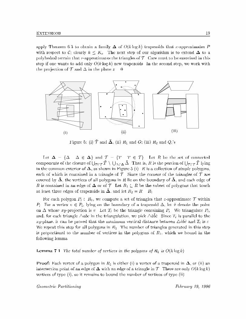
(i) (ii) (iii)Figure 5: (i) �T and ��, (ii) R1 and G; (iii) R2 and Qi's.Let �� = f �� j � 2 �g and �T = f �T j T 2 T g. Let R be the set of connectedcomponents of the closure of ST2T �T n S�2� ��. That is, R is the portion of ST2T �T lyingin the common exterior of ��, as shown in Figure 5 (i). R is a collection of simple polygons,each of which is contained in a triangle of �T . Since the corners of the triangles of �T arecovered by ��, the vertices of all polygons in R lie on the boundary of ��, and each edge ofR is contained in an edge of �� or of �T . Let R1 � R be the subset of polygons that touchat least three edges of trapezoids in ��, and let R2 = R�R1.For each polygon Pi 2 R1, we compute a set of triangles that "-approximate T withinPi. For a vertex v 2 Pi, lying on the boundary of a trapezoid ��, let v denote the pointon � whose xy-projection is v. Let �Ti be the triangle containing Pi. We triangulate Pi,and, for each triangle 4abc in the triangulation, we pick 4abc. Since Ti is parallel to thexy-plane, it can be proved that the maximum vertical distance between 4abc and Ti is ".We repeat this step for all polygons in R1. The number of triangles generated in this stepis proportional to the number of vertices in the polygons of R1, which we bound in thefollowing lemma.Lemma 7.1 The total number of vertices in the polygons of R1 is O(k log k).Proof: Each vertex of a polygon in R1 is either (i) a vertex of a trapezoid in ��, or (ii) anintersection point of an edge of �� with an edge of a triangle in T . There are only O(k log k)vertices of type (i), so it remains to bound the number of vertices of type (ii).Geometric Partitioning February 19, 1996

Extensions 20We construct an undirected graph G = (V;E), as follows. Let � = f 1; : : : ; tg be theset of edges in ��.1 To avoid confusion, we will call the edges of � segments and those of Earcs. For each segment i, we place a point i close to i, inside the trapezoid bounded by i. The set of resulting points forms the node set V . If there is an edge pq of a polygon inR1 such that p 2 i and q 2 j , we add the arc (i; j) to E; see Figure 5 (ii). It is easily seenthat G is a planar graph, and that jEj = O(k log k). Fix a pair of segments 1; 2 2 � suchthat (1; 2) 2 E. Let E12 = fp1q1; p2q2; : : :g be the set of edges in R1, sorted either left toright or top to bottom, as the case may be, that are incident to 1 and 2. Let jE12j = mij .Assume that for every 1 � i � mij, pi lies on 1 and qi lies on 2. The number of verticesof type (ii) is obviously 2P(i;j)2E mij. We call two edges piqi; pjqj 2 E12 equivalent if theinterior of the convex hull of piqi and pjqj does not intersect any trapezoid of ��. Thisequivalence relation partitions E12 into equivalent classes, each consisting of a contiguoussubsequence of E12. Let �ij denote the number of equivalence classes in Eij.Claim 1: There are at most two edges in each equivalence class of E12.Proof: Assume for the sake of a contradiction that three edges pi�1qi�1; piqi and pi+1qi+1belong to an equivalence class. Further, assume that the triangle �T 2 �T bounded by piqilies below piqi (see Figure 6 (i)). Since the quadrilateral Q de�ned by piqi and qi+1pi+1does not contain any trapezoid of ��, pi+1qi+1 is also an edge of �T and Q � �T . But then Qis a connected component of R and it touches only two edges of ��, thereby implying thatpiqi is not an edge of a polygon of R1, a contradiction. 2Thus,X(i;j)2Emij � 2 X(i;j)2E �ij = 2jEj+ X(i;j)2E(�ij � 1) = O(k log k) + X(i;j)2E(�ij � 1) :Next, we bound the quantity P(i;j)2E(�ij � 1). Let Ej12 and Ej+112 be two consecutiveequivalent classes of E12, let piqi be the bottom edge of Ej12, and let pi+1qi+1 be the topedge of Ej+112 . The quadrilateral Qj12 = piqiqi+1pi+1 contains at least one trapezoid �� of ��.We call piqi; pi+1qi+1 the triangle edges of Q, and pipi+1; qiqi+1 the trapezoidal edges of Q.The triangle edges of Qj12 are adjacent in E12. Let Q = SfQlij j (i; j) � E and l < �ijg bethe set of resulting quadrilaterals. Since jQj = P(i;j)2E(�ij � 1), it su�ces to bound thenumber of quadrilaterals in Q.Consider the planar subdivision induced by Q and call it A(Q). For each bounded facef 2 A(Q), let Q(f) be the smallest quadrilateral of Q that contains f . Since the boundariesof quadrilaterals do not cross, Q(f) is well de�ned.Claim 2: Every face f of A(Q) can be uniquely associated with a trapezoid � 2 �� such1The segments of � may overlap, because the trapezoids of �� can touch each other. If a segment i of� is an edge of two trapezoids, then no edge of R1 can be incident to i.Geometric Partitioning February 19, 1996

Extensions 21QiQj(ii)pi qi+1qiqi�1(i)

pi�1pi+1 1 2 pi

pi+1 qi+1qi

1 2��Figure 6: (i) Edges in an equivalent class of E12, and (ii) edges in di�erent equivalent classesthat � � f .Proof: The claim is obviously true for the unbounded face, so assume that f is a boundedface. If Qi = Q(f) does not contain any other quadrilateral of Q, then f = Qi, and so byde�nition f contains a trapezoid of ��. If Qi = Q(f) does contain another quadrilateralof Q, let Qj be the largest trapezoid that lies inside Qi|that is, @Qj is a part of @f . Ifnone of the trapezoidal edges of Qj lies in the interior of Qi, then the trapezoidal edges ofboth Qi; Qj lie on the same segments of �, say, 1; 2. Consequently, the triangle edges ofboth Qi; Qj belong to E12, which is impossible because then the triangle edges of Qi arenot adjacent in E12. Hence, one of the trapezoidal edges of Qj lies in the interior of Qi. Let�� be the trapezoid bounded by this edge. Since the triangle edges of Qj lie outside �� andthe interior of �� does not intersect any edge of R1, �� lies in f . This completes the proofof Claim 2. 2By Claim 2, the number of faces in A(Q) is at most j ��j = O(k log k). This completesthe proof of the lemma. 2Next, we partition the polygons of R2 into equivalence classes in the same way as wepartitioned the edges of E12 in the proof of Lemma 7.1. That is, we call two polygons�1; �2 2 R2 equivalent if (i) their endpoints lie on the same pair of edges in ��, and (ii) theinterior of the convex hull of �1 [ �2 does not intersect any trapezoid of ��. Using the sameargument as in the proof of the above lemma, the following lemma can be established.Lemma 7.2 The edges of R2 can be partitioned into O(k log k) equivalence classes.For each equivalence class Ei � R2, let Qi be the convex hull of Ei|observe that Qiis a convex quadrilateral, as illustrated in Figure 5 (iii). Each quadrilateral Qi can be "-approximated using at most three triangles in R3 in the same way as we approximated eachGeometric Partitioning February 19, 1996

Closing Remarks 22polygon Pi of R1. By Lemma 7.2, the total number of triangles created in this step is alsoO(k log k).Putting together these pieces, we obtain the following lemma.Lemma 7.3 The family of trapezoids � can be supplemented with O(k log k) additionaltrapezoids in R3 so that all the triangles of T are "-approximated. The orthogonal projectionof all the trapezoids on the plane z = 0 is pairwise disjoint.The area not covered by the projection of trapezoids found in the preceding lemma, ofcourse, can be approximated without any regards to the triangles of T . The �nal surfacehas O(Ko logKo) trapezoids and it "-approximates the family of triangles T . We �nish witha statement of our main theorem in this section.Theorem 7.4 Given a set of n horizontal triangles in R3 , with pairwise disjoint projectionon the plane z = 0, and a parameter " > 0, we can compute in polynomial time a "-approximate polyhedral terrain of size O(Ko logKo) for T , where Ko is the size of an optimal"-approximate terrain.8 Closing RemarksWe presented an approximation technique for certain geometric covering problems witha disjointness constraint. Our algorithm achieves a logarithmic performance guaranteeon the size of the cover, thus matching the bound achieved by the \greedy set cover"heuristic for arbitrary sets and no disjointness constraint. Applications of our result includepolynomial time algorithms to approximate a monotone, polyhedral surface in 3-space, andto approximate the disjoint cover by triangles of red-blue points. We also proved that theseproblems are NP-Hard .The surface-approximation problem is an important problem in visualization and com-puter graphics. The state of theoretical knowledge on this problem appears to be ratherslim. Except for the convex surfaces, no approximation algorithms with good performanceguarantees are known [7, 17]. For the approximation of convex polytopes, it turns out thatone does not need disjoint covering, and therefore the greedy set cover heuristic works.We conclude by mentioning some open problems. An obvious open problem is to re-duce the running time of our algorithm for it to be of any practical value. Finding e�cientheuristics with good performance guarantees seems hard for most of the geometric parti-tioning problems, and requires further work. A second problem of great practical interestis to "-approximate general polyhedra|this problem arises in many real applications ofcomputer modeling. To the best of our knowledge, the latter problem remains open evenGeometric Partitioning February 19, 1996

References 23for the special case where one wants to �nd a minimum-vertex polyhedral surface that liesbetween two monotone surfaces. The extension of our algorithm presented in Section 7 doesnot work because we do not know how to handle the last �ll-in stage.AcknowledgmentsThe authors thank Joe Mitchell, Prabhakar Raghavan, and John Reif for several helpfuldiscussions.References[1] E. Allgower and S. Gnutzmann, An algorithm for piecewise linear approximation of an im-plicitly de�ned two-dimensional surfaces, SIAM J. Numerical Analysis 24 (1987), 452{469.[2] E. Allgower and P. Schmidt, An algorithm for piecewise linear approximation of an implicitlyde�ned manifold, SIAM J. Numerical Analysis 22 (1985), 322{346.[3] E. Arkin, H. Meijer, J. Mitchell, D. Rappaport, S. Skiena, Decision trees for geometric models,Proceedings 9th Annual Symposium on Computational Geometry, 1993, 369{378.[4] J. Bloomenthal, Polygonization of implicit surfaces, Computer Aided Design 5 (1988), 341{355.[5] H. Br�onnimann and M. T. Goodrich, Almost optimal set covers in �nite VC-dimension, Proc.10th ACM Symp. on Computational Geometry, 1994, pp. 293{302.[6] B. Chazelle and M. Sharir and E. Welzl, Quasi-optimal upper bounds for simplex rangesearching and new zone theorems, Algorithmica, 8 (1992), 407{429.[7] K. L. Clarkson, Algorithms for polytope covering and approximation, Proc. 3rd Workshopon Algorithms and Data Structures , Lectures Notes in Computer Science, vol. 709, SpringerVerlag, pp. 246{252, 1993.[8] M. DeHaemer and M. Zyda, Simpli�cation of objects rendered by polygonal approximations,Computers and Graphics 15 (1992), 175{184.[9] S. Fekete, Several hardness results on problems of point separation and line stabbing, Tech.Report, Department of Applied Mathematics and Statistics, SUNY Stony Brook, 1993.[10] R. Fowler, M. Paterson, and L. Tanimoto, Optimal packing and covering in the plane areNP-complete, Information Processing Letters 35 (1981), 85{92.[11] I. Ihm and B. Naylor, Piecewise linear approximations of digitized space curves with applica-tions Scienti�c Visualization of Physical Phenomena pp. 545{569, Springer{Verlag, 1991.[12] D. S. Johnson., Approximation algorithms for combinatorial problems, Journal of Computerand System Sciences , (1974), 256{278.Geometric Partitioning February 19, 1996

References 24[13] D. Lichtenstein, Planar formulae and their uses, SIAM J. Computing 11 (1982), 329{343.[14] W. Lorenson and H. Cline, Marching cubes: A high resolution 3D surface construction algo-rithm, Computer Graphics 21 (1987), 163{169.[15] L. Lov�asz, On the ratio of optimal integral and fractional cover, Discrete Mathematics 13(1975), 383{390.[16] N. Megiddo, Linear-time algorithms for linear programming in R3 and related problems, SIAMJ. Computing 12 (1983), 759{776.[17] J. Mitchell and S. Suri, Separation and approximation of polyhedral surfaces, Proc. of 3rdACM-SIAM Symposium on Discrete Algorithms (1992), 296{306.[18] M. S. Paterson and F. F. Yao, E�cient binary space partitions for hidden-surface removaland solid modeling, Discrete and Computational Geometry , 5 (1990), 485{503.[19] M. S. Paterson and F. F. Yao, Optimal binary space partitions for orthogonal objects, J.Algorithms 13 (1992), 99{113.[20] F. P. Preparata and M. I. Shamos, Computational Geometry: An Introduction, Springer-Verlag, 1985.[21] S. Salzberg, R. Chandar, H. Ford, S. Murthy, and R. White, A survey of decision tree classi�ermethodology, IEEE Trans. Systems, Man and Cybernatics 21 (1991), 660{674.[22] W. Schroeder, J. Zarge, and W. Lorensen, Decimation of triangle meshes, Computer Graphics26 (1992), 65{78.[23] F. Schmitt, B. Barsky, and W. Hui Du, An adaptive subdivision method for surface �ttingfrom sampled data, Computer Graphics 20 (1986), 179{188.[24] S. Suri, On some link distance problems in a simple polygon, IEEE Transactions on Roboticsand Automation, 6 (1) (1990), 108{113.[25] G. Turk, Re-tiling of polygonal surfaces, Computer Graphics 26 (1992), 55{64.

Geometric Partitioning February 19, 1996