empirical results on the generalization capabilitie sand · zing the margin (as with the svm), the...

Empirical Results on the Generalization Capabilities and

Convergence Properties of the Bayes Point Machine

Sumit Basu

Perceptual Computing Section, The MIT Media Laboratory

20 Ames St., Cambridge, MA 02139 USA

[email protected]

We explore some of the convergence and generalization properties of the Bayes Point Machine (BPM) developed

by Herbrich [3], an alternative to the Support Vector Machine (SVM) for classi�cation. In the separable case,

there are an in�nite number of hyperplanes in version space that will perfectly separate the data. Instead of

choosing a solution based on maximizing the margin (as with the SVM), the BPM seeks an approximation to

the Bayes Point, the point in version space that is closest in behavior to the Bayes integral over all hyperplanes.

Herbrich approximates this point using a stochastic algorithm for an arbitrary kernel (the billiard algorithm)

which bounces a ball around the version space in order to estimate the Bayes Point. Because many kernels imply

in�nite dimensional feature spaces, it is interesting to investigate how long such an algorithm must run before it

will converge. In a series of experiments on separable data (i.e., separable in the feature space), we thus test the

BPM algorithm with a polynomial kernel (low-dimesional) and a RBF kernel (in�nite dimensional). We compare

generalization results with the SVM, investigate convergence rates, and examine the di�erence between the BPM

and SVM solutions under several data conditions. We �nd that the BPM does converge rapidly and tightly

even for in�nite dimensional kernel, and that it has signi�cantly better generalization performance only when the

number of support vectors is of medium value with respect to the number of training points (i.e., more often with

low-dimensional kernels). In addition, we augment Herbrich's discussion with some comments on the bias term,

corrections to his pseudocode, and a MATLAB implementation of his algorithm to be made publicly available.

1 Introduction

In the conventional classi�cation problem, we seek a hyperplane w that separates the data in some feature

space such that our classi�er f(x) is of the following form:

f(x) = sign(wTx) (1)

Since wTx is simply a scalar, we can replace the conceptual roles of w and x: just as a particular point w

de�nes a hyperplane in the feature space, a particular x de�nes a hyperplane in parameter space. Each such

Perceptual Computing

Sumit Basu. "Empirical Results on the Generalization Capabilities and Convergence Properties of the Bayes Point Machine." Technical Report. December, 1999.

hyperplane produces a constraint in version space, where a valid solution must be on one side of the plane or the

other. If the data are separable, the intersection of all of these constraints results in a convex hull in parameter

space referred to as version space (see �gure 1).

Figure 1: An illustration of a solution polyhedron in version space. The cross indicates the center of the largestinscribable hypersphere (the SVM solution), while the star indicates the center of mass solution (approximatedby the BPM).

Since any solution in this polyhedron will perfectly separate the training data, we need additional constraints

to choose a unique solution. Ignoring the bias term for the moment, the Support Vector Machine (SVM) [6]

approach is to minimize kwkF (where F is the feature space) subject to:

yi < w;�(xi) >F� 1; i = 1; :::; l (2)

where l is the number of training examples (see, for example, [3]). This can be interpreted as �nding the

largest hypersphere that can be inscribed within the polyhedron: we are looking for the w of minimum norm

such that the distance from the origin to each constraint hyperplane is at least 1 (see �gure 1). The \support

vectors" are then the constraint hyperplanes where this distance is exactly 1, i.e., where the hypersphere touches

the polyhedron.

The Bayesian solution, on the other hand, does not result in the choice of a single w, but instead \votes" the

outputs of all valid solutions over the volume of the polyhedron, i.e.,

fBayes(x; p(w)) = sign(

Zw2V(S)

sign(< w;�(x) >)p(w)) (3)

= sign(Ep(w)[sign(< w;�(x) >)]) (4)

where V(S) is the version space and p(w) is a prior over the space. Since in general we do not have any

additional information about the possible distribution of hyperplanes, we choose a uniform prior. However, note

it could be interesting to use this prior as a means of encoding past experience about the problem. With a uniform

prior, if we separate the possible classi�ers in V(S) for a given x into those that will classify it as positive and

those that will classify it as negative, it is fairly easy to see that their combined output in the Bayesian classi�er

2

will be the sign of the set that occupies the larger volume in version space. Note, however, that the resulting

classi�er, is not guaranteed to be in the version space, i.e., we cannot in general represent it with a single w.

Furthermore, a means of explicitly computing the volume integrals, even in the case of the uniform prior, has

not been found analytically. A numerical solution is not a possibility here, since many kernels result in in�nite

dimensional features spaces and thus version spaces.

As a result, previous researchers have sought after the \Bayes point," the point in version space which most

closely approximates the behavior of the optimal Bayes classi�er in an L2 sense [3]:

fbp = argminf2V(S)

Z(fBayes(x; p(w))� fbp(x))

2p(x)dx (5)

Watkin [8] and Opper [4] have shown that the center of mass of the version space wcm (i.e., the expectation

of w over the version space) converges to the Bayes point solution at a fast rate. Watkin and others refer to this

point as the \optimal perceptron." The resulting classi�er can be written as

fcm(x; p(w)) = sign(

Zw2V(S)

< w;�(x) >)p(w)dw (6)

= sign(Ep(w)[< w;�(x) >]) (7)

= sign(< Ep(w)[w];�(x) >]) (8)

(Note that the interpretation as an expectation is my own). Thus, instead of voting the outputs of each possible

classi�er (as in equation 4), we are now voting the raw outputs of the inner products with each w.

Still, we are left with the signi�cant problem of �nding the center of mass of the version space. Once again, no

analytic solution is known to this problem, even under a uniform prior over version space. Rujan [5] developed a

\billiard" algorithm that bounces a ball about in version space to estimate its center of mass (in the uniform prior

case). In most cases, the billiard's path results in a uniform coverage of version space. He shows the convergence

properties of the algorithm empirically, but notes that it is not possible to prove that a given polyhedron will be

ergodic, i.e., that the billiard's path will cover the space uniformly. He gives some examples (such as an ellipse)

that will not be covered uniformly, but also mentions that the irregular shapes resulting from the data constraints

of a classi�cation problem are unlikely to have the sort of symmetry necessary to break ergodicity.

Rujan's algorithm, though, was implemented directly in the version space. This was �ne for linear hyper-

planes, where the dimensionality of feature space is simply the dimensionality of the data. However, it is

di�cult/impossible when kernels are involved. Many kernels result in very high dimensional (often in�nite di-

mensional) feature spaces, rendering Rujan's algorithm intractable. Ralf Herbrich, in very recent work [3] has

3

developed a clever new billiard algorithm (which he terms the Bayes Point Machine, or BPM) in which points in

the version space do not have to be explicitly represented, given again that we have a uniform prior over version

space. As a result, his algorithm is applicable to feature spaces of arbitrary dimension.

However, this still leaves a major question - how long does it take the billiard algorithm to converge when

it is operating in in�nite dimesional spaces? Herbrich comes up with some impressively tight bounds that are

training data-dependent, but these all depend on �nding the volume of the version space polyhedron, which is

di�cult/impossible to estimate. Rujan argues that his algorithm should take O(N2) collisions to converge for

N�dimensional data. That implies Herbrich's algorithm should take in�nite time to converge for some kernels

- yet he gives impressive generalization results on the standard databases, giving no comment on how long

convergence took.

This study thus sets out to investigate the convergence properties of Herbrich's kernel billiard algorithm. We

have implemented the algorithm in MATLAB (the code is at the end of this document, and will be made publicly

available on the web), �xing a number of bugs and omissions in Herbrich's pseudocode. We now use this to

look at the convergence properties of the algorithm in terms of speed, performance, and distance from the SVM

solution across varying kernel dimensionalities, dataset dimensionalities, and data distributions.

2 Billiards in a RKHS

In this section, we describe Herbrich's representation and framework, and then comment on some aspects of

implementing the algorithm.

Herbrich's representation/notation for operations in reproducing kernel Hilbert spaces (RKHS) mostly follows

that of Grace Wahba [7], adding the \feature space" interpretation of the SVM world [6]. First, we have a

mapping, �(x) (with vector output) which maps from the data space X to the feature space F , typically of a

higher dimensionality. We then have a kernel, K(�; �) such that

K(x; y) =< �(x);�(y) >F (9)

Note that this mapping function is not to be confused with the �i(�) used to represent the orthogonal decom-

position of the kernel. We know (i.e., [6]) that any solution in the hypothesis space (again neglecting the bias

term) can be represented in the following way:

f(x) =

lXi=1

�iK(x; xi) (10)

We can thus rewrite this as an inner product in feature space:

4

f(x) = < w;�(x) > (11)

w =

lXi=1

�i�(xi) (12)

This can be seen by a simple rearrangement of terms. While the latter representation can often not be

represented explicitly (i.e., when F is of in�nite dimension), it is theoretically useful in that it is the space in

which we will be bouncing about the billiard. Furthermore, we can take the inner product between two elements

in F that have the form of w in equation 12 as

< a; b >=<

lXi=1

�i�(ai);

lXj=1

�i�(bj) > =

lXi=1

lXj=1

�i�jK(xi; xj) (13)

= �TK� (14)

and we can �nd the norm of a vector that can be represented in this way as

kakF = �TK� (15)

where K is a matrix such that Kij = K(xi; xj). Since we know K(i; j) is positive de�nite, K is also positive

de�nite, and thus < a; b > and the norms (i.e., kak) are always positive if a; b are non-zero.

Furthermore, Herbrich constrains his solutions to be on the surface of the unit hypersphere, i.e., kwk = 1,

which makes it possible for him to develop his billiard algorithm. If we neglect the bias term (which we've been

conveniently neglecting all along), this is not a problem: we are then only looking at the sign of < w;�(x) >,

and the magnitude of w makes no di�erence (all the hyperplanes still pass through the origin). Most kernels have

an \implicit bias" and thus do not need an additional bias term (an \explicit bias") [2]. Some, like the simple

inner product (K(x; y) =< x; y >) do need an explicit bias. However, we can get around this by simply adding

\1" to the kernel function, so K(x; y) =< x; y > +1 - we in fact use this kernel (also known as the �rst order

polynomial kernel) in many of our experiments below. Gunn [2] shows that this added-in implicit bias does not

result in the same solution as the explicit bias, but gives the same exibility and similar performance. Girosi [1]

states that any �nite kernel can be expanded in this way; however, there does not seem to be any reason that it

can't be used on an in�nite kernel, since adding 1 to any kernel function will retain its positive de�niteness.

The beauty of Herbrich's algorithm is that all calculations can be done in the dimensionality of the number

5

of data points instead of the dimensionality of the kernel. Every representation and update for a vector a in

feature space is simply done in terms of the corresponding coe�cients, �i. I will not go through the details of the

algorithm here, since Herbrich's report [3] already does this, but I will give a brief outline of the steps involved.

Remember that the version space is now on the surface of a hypersphere in a Hilbert space F . The constraint

hyperplanes all pass through the origin (the centroid of the hypersphere) and cut through the hypersphere. We

will then �nd the solution by bouncing a billiard between these constraints. In 3D, the hypersphere would be a

sphere, and the (2D) planes of constraint would cut great circles on the surface of the sphere. We would then

have a polyhedron of the form of �gure 1 on the surface of the sphere.

To begin the process, we need to �nd a valid solution that lies within the version space. We use SVM to

do this, but any kernel learning algorithm that can �nd the solution will do. Given a solution, we choose a

random direction for the billiard to travel in. We then go through all the hyperplanes (one per training example),

calculating how long it will be before we hit each and �nd the point of intersection on the closest one (note that

we must consider all hyperplanes, not just those corresponding to the support vectors, since we typically have

the situation of �gure 1). It would be very di�cult to do this on the actual surface of the hypersphere, but

Herbrich cleverly takes advantage of the fact that closest hyperplane is the same for a linear trajectory along the

tangent to the hypersphere as for a trajectory along the surface. We thus �nd the intersection point along this

linear trajectory and then normalize the point to �nd the projection onto the hypersphere. We then compute the

midpoint between the previous location of billiard and the current point, and compute a new overall midpoint by

taking a weighted average (specially constrained to lie on the hypersphere) between the overall midpoint computed

thus far and the new segment's midpoint. The weights are determined by the the total path length traversed

by the billiard and the length of the latest segment, respectively. We then reverse the direction of the billiard

for the component along the normal to the hyperplane and continue the iteration. Herbrich advises a stopping

point based on an upper bound on the weight for the midpoint of the new segment. In this study, however, since

we were interested in the convergence properties, we run the algorithm for a pre-speci�ed number of bounces. It

would be a trivial modi�cation of the MATLAB code supplied to use Herbrich's condition.

Unfortunately, Herbrich's paper and pseudocode has a number of errors - some small, some signi�cant. There

are also some things he neglects to mention - for example, when the billiard bounces o� of a particular hyperplane,

it is necessary to ensure that the next bounce is o� of a di�erent hyperplane - otherwise, numerical errors will

have the billiard bouncing back and forth around the same constraint. Another important point is that his

representation of the coe�cients �i that represent the hyperplane are signed, i.e., they incorporate the value of

yi, as opposed to the usual SVM formulation in which the �'s are all positive and are multiplied by the yi's during

computations. We hope to have corrected all of these in our MATLAB implementation, but undoubtedly some

bugs have gotten through. If you �nd any errors, please email them to us at [email protected].

6

3 Experiments and Results

In the following experiments, we look at the performance of two kernels: the �rst order polynomial,K(x; y) =<

x; y > +1, and the rbf kernel K(x; y) = exp((x�y)T (x�y)

2�2 ) with � = 1. The �rst is a low dimensional kernel

(dimensionality of the data plus one) and the latter has an in�nite dimensional feature space. Both have an

implicit bias.

Since we are working with the separable version of the algorithm, we needed to create a number of linearly

separable datasets. We did this following the method of Rujan [5]: a set of 100 points of uniformly distributed

data was generated in RN ; then a set of signed coe�cients �i was made, resulting in a classi�er

f(x) = sign(

lXi=1

�iK(x; xi)) (16)

where K is the kernel being considered, which was used to separate the data. The resulting dataset was thus

guaranteed to be separable by this kernel. For each of the experiments below, the data were split in a 60/40 ratio

for training and test in 10 di�erent ways. The results shown are all averages (and standard deviations) taken over

these 10 trials.

3.1 Convergence Times

This �rst experiment shows the convergence rate of the billiard algorithm for two dimensionalities of data and

feature spaces. All of the plots in �gures 2 and 3 show the log (base 10) of average change of the L1 norm of

coe�cients � for w =P

�i�(xi), average over the last 100 or so trials with an IIR �lter y[i] = 0:99y[i�1]+0:01x[i].

0 0.5 1 1.5 2 2.5 3 3.5 4 4.5 5

x 104

−4.5

−4

−3.5

−3

−2.5

−2

−1.5

−1

−0.5

0

number of trials

log1

0(ru

nnin

g av

g of

L1

chg

in a

lpha

)

0 0.5 1 1.5 2 2.5 3 3.5 4 4.5 5

x 104

−5.5

−5

−4.5

−4

−3.5

−3

−2.5

−2

−1.5

−1

−0.5

number of trials

log1

0(ru

nnin

g av

g of

L1

chg

in a

lpha

)

Figure 2: log(��) vs. number of bounces for the billiard algorithm on 5-dimensional data using a polynomialkernel (left, 6 support vectors out of 60) and an rbf kernel (right, 25 support vectors out of 60).

These �gures give us some reassuring results. Note that the change in � drops by three order of magnitude in

20,000 bounces, and signi�cantly more than this most cases. As a result, we can be sati�ed that even in in�nite

7

0 0.5 1 1.5 2 2.5 3 3.5 4 4.5 5

x 104

−6

−5.5

−5

−4.5

−4

−3.5

−3

−2.5

−2

−1.5

−1

number of trials

log1

0(ru

nnin

g av

g of

L1

chg

in a

lpha

)

0 0.5 1 1.5 2 2.5 3 3.5 4 4.5 5

x 104

−8

−7

−6

−5

−4

−3

−2

−1

number of trials

log1

0(ru

nnin

g av

g of

L1

chg

in a

lpha

)

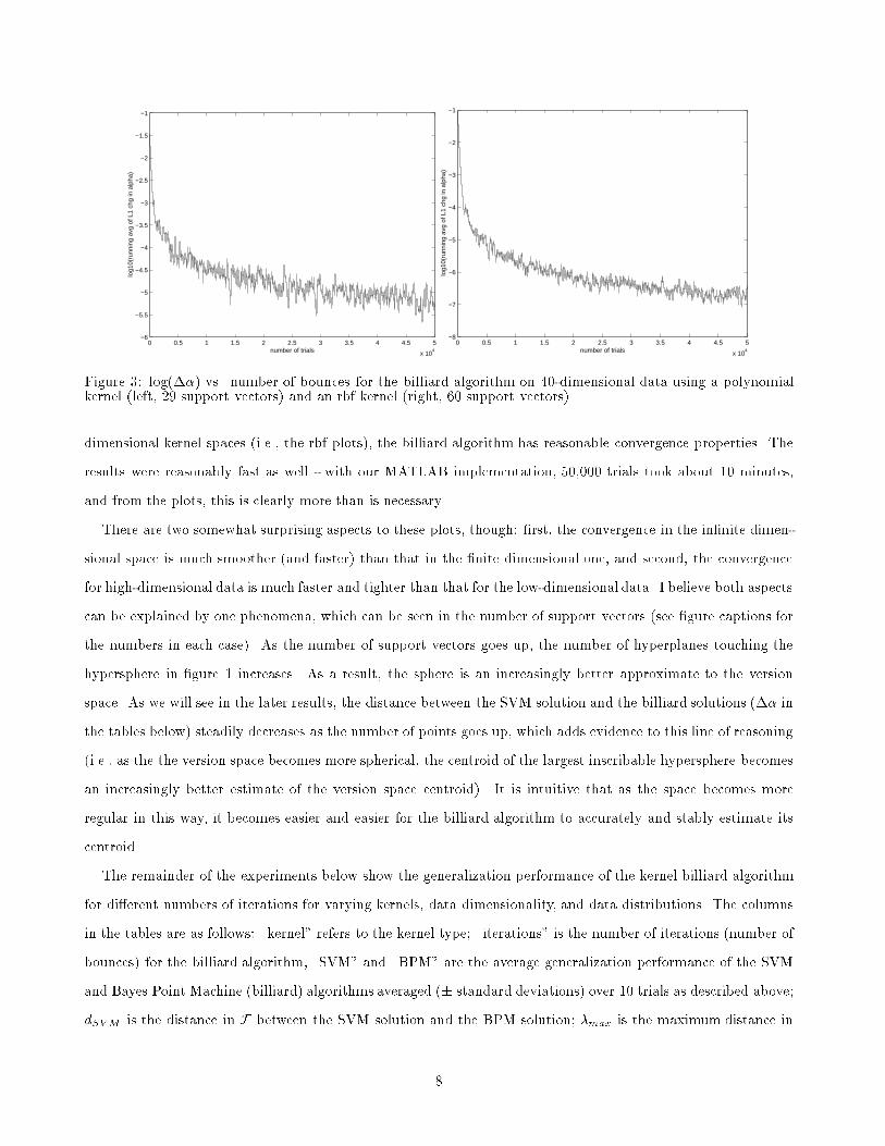
Figure 3: log(��) vs. number of bounces for the billiard algorithm on 40-dimensional data using a polynomialkernel (left, 29 support vectors) and an rbf kernel (right, 60 support vectors).

dimensional kernel spaces (i.e., the rbf plots), the billiard algorithm has reasonable convergence properties. The

results were reasonably fast as well - with our MATLAB implementation, 50,000 trials took about 10 minutes,

and from the plots, this is clearly more than is necessary.

There are two somewhat surprising aspects to these plots, though: �rst, the convergence in the in�nite dimen-

sional space is much smoother (and faster) than that in the �nite dimensional one, and second, the convergence

for high-dimensional data is much faster and tighter than that for the low-dimensional data. I believe both aspects

can be explained by one phenomena, which can be seen in the number of support vectors (see �gure captions for

the numbers in each case). As the number of support vectors goes up, the number of hyperplanes touching the

hypersphere in �gure 1 increases. As a result, the sphere is an increasingly better approximate to the version

space. As we will see in the later results, the distance between the SVM solution and the billiard solutions (�� in

the tables below) steadily decreases as the number of points goes up, which adds evidence to this line of reasoning

(i.e., as the the version space becomes more spherical, the centroid of the largest inscribable hypersphere becomes

an increasingly better estimate of the version space centroid). It is intuitive that as the space becomes more

regular in this way, it becomes easier and easier for the billiard algorithm to accurately and stably estimate its

centroid.

The remainder of the experiments below show the generalization performance of the kernel billiard algorithm

for di�erent numbers of iterations for varying kernels, data dimensionality, and data distributions. The columns

in the tables are as follows: \kernel" refers to the kernel type; \iterations" is the number of iterations (number of

bounces) for the billiard algorithm, \SVM" and \BPM" are the average generalization performance of the SVM

and Bayes Point Machine (billiard) algorithms averaged (� standard deviations) over 10 trials as described above;

dSVM is the distance in F between the SVM solution and the BPM solution; �max is the maximum distance in

8

F between two bounces in the billiard algorithm, which gives a sense of the size of the solution polyhedron and

thus an interpretation for dSVM ; NSV is the number of support vectors (out of 60 possible training points); and

�� is the running average of the L1 norm of the change in � at the end of the trial (as in the plots above), which

gives us a sense of how far the algorithm has converged. Note that each table corresponds to a di�erent dataset

(created to be separable for that kernel, as described above), and each row of the table represents an average over

10 di�erent divisions of that dataset into training (60%) and test (40%) sets.

3.2 Performance vs. Data Dimensionality

This set of experiments shows the variation in performance over di�erent dimensionalities of training data.

Table 1 and 2 show the performance for 5 dimensional data, while tables 4 and 4 show the results for 40 dimensional

data.

Table 1: Results for the polynomial kernel on 5 dimensional data, averaged over 10 trials for each row, with 60training and 40 test examples.

kernel iterations SVM BPM dSVM �MAX NSV ��

poly 50 96.25 � 2.70 94.25 � 4.72 0.0819 0.3194 5.8 1.13e-001poly 100 98.50 � 1.75 97.25 � 1.42 0.1001 0.2942 5.7 8.95e-002poly 500 96.25 � 2.70 96.00 � 3.16 0.1161 0.3705 6.0 1.59e-002poly 1000 95.25 � 3.99 94.25 � 3.55 0.1240 0.4696 5.8 4.41e-003poly 5000 94.75 � 4.48 95.00 � 3.54 0.1119 0.5474 5.6 7.52e-004poly 10000 97.00 � 2.84 96.50 � 2.93 0.0833 0.5528 5.9 4.43e-004poly 50000 97.00 � 3.07 96.00 � 3.57 0.0915 0.5998 5.9 8.43e-005

Table 2: Results for the rbf kernel on 5 dimensional data, averaged over 10 trials for each row, with 60 trainingand 40 test examples.


rbf 50 97.00 � 2.84 97.50 � 2.64 0.6057 0.7705 18.6 6.24e-002rbf 100 95.75 � 3.13 98.75 � 2.43 0.5373 0.9609 17.5 4.92e-002rbf 500 97.75 � 1.84 98.75 � 2.12 0.5637 0.9993 18.2 4.38e-003rbf 1000 98.75 � 2.12 100.00 � 0.00 0.5523 1.0182 17.9 1.40e-003rbf 5000 96.00 � 2.93 98.50 � 2.69 0.5397 1.1859 17.7 1.65e-004rbf 10000 97.00 � 2.84 99.50 � 1.58 0.5695 1.2211 17.7 9.07e-005rbf 50000 97.50 � 3.12 99.50 � 1.58 0.5697 1.2570 17.0 1.19e-005

In the �rst set of experiments (5-dimensional data, polynomial kernel, table 1), the number of support vectors

is small, and as we expect from our conjectures in the previous experiments, the distance between the SVM and

BPM solutions is relatively large. However, the generalization performance of the two algorithms is similar, and

in fact slightly worse for the polynomial kernel. I do not have a good explanation for this at the time, but perhaps

though the � seemed to converge, the small number of boundaries (support vectors) of the solution subspace

somehow makes the billiard less capable of accurately estimating the center of mass. For the same type of data

(5-dimensional data, rbf kernel, table 2), the billiard algorithm does signi�cantly better than the SVM. The

9

number of support vectors here is much larger, but the distance from the SVM solution is still signi�cant. Given

what we have seen this far, this gives the billiard algorithm a large space to bounce around in with a good many

constraints, but still di�erent enough from the spherical approximation to make the center of mass estimate a

better performer.

Table 3: Results for the polynomial kernel on 40 dimensional data, averaged over 10 trials for each row, with 60training and 40 test examples.



Table 4: Results for the rbf kernel on 40 dimensional data, averaged over 10 trials for each row, with 60 trainingand 40 test examples.


rbf 50 45.50 � 8.06 41.75 � 6.13 0.3779 0.5267 60.0 4.99e-002rbf 100 51.00 � 9.52 47.50 � 9.28 0.3214 0.5219 60.0 3.18e-002rbf 500 49.25 � 5.90 48.00 � 5.87 0.1588 0.5557 60.0 9.22e-004rbf 1000 46.50 � 8.10 46.75 � 7.46 0.1068 0.5361 60.0 8.06e-005rbf 5000 47.50 � 5.89 47.00 � 5.75 0.0478 0.5321 60.0 4.50e-006rbf 10000 42.50 � 7.26 41.75 � 7.27 0.0346 0.5531 60.0 1.50e-006rbf 50000 45.00 � 3.12 45.00 � 3.73 0.0166 0.5572 60.0 0.00e+000

In the second set of experiments, we see more what we expect. For the 40-dimesional data, polynomial kernel

case (table 3), we now have a fair number of support vectors, though far less than 100% (as we did in the case

with the 5-dimensional data and the rbf kernel), so the distance from the SVM solution is still signi�cant. As

a result, we again see excellent generalization performance - the BPM always does better than the SVM. For

the rbf case with 40-dimensional data, though (rable 4), we see precisely the same performance as the number of

iterations goes up. This is easy to understand given what we have seen so far - 100% of the data are now being

used as support vectors, which means the spherical approximation to the hypersphere is an excellent one. As a

result, the billiard algorithm, given enough iterations, is converging to the same solution as the SVM. This is

made clear by the miniscule relative distance between the BPM and SVM solutions.

3.3 Performance vs. Data Distribution

This last set of experiments shows the performance of the algorithms under di�erently shaped datasets. This

was motivated by the conjecture that that uniform distribution of the points in the dataset may have led to the

apparent spherical nature of the previous experiments, thus resulting in such a large number of support vectors for

10

the rbf kernel. Tables 5 and 6 show the performance for a dataset that is uniformly distributed in all dimensions

except for the �rst, which is scaled by a factor of 10 in terms of the others.

Table 5: Results for the polynomial kernel on 40 dimensional data stretched by a factor of 10 along one dimension,averaged over 10 trials for each row, with 60 training and 40 test examples.



Table 6: Results for the rbf kernel on 40 dimensional data stretched by a factor of 10 along one dimension,averaged over 10 trials for each row, with 60 training and 40 test examples.


rbf 50 51.50 � 8.68 52.50 � 9.13 0.3118 0.1103 47.6 2.02e-001rbf 100 55.00 � 8.25 56.75 � 8.42 0.3965 0.1137 49.2 1.31e-001rbf 500 53.50 � 4.74 51.75 � 5.53 0.3218 0.1366 49.1 5.36e-003rbf 1000 49.25 � 6.02 49.50 � 6.85 0.2799 0.1681 48.8 1.18e-003rbf 5000 56.00 � 8.76 53.75 � 5.68 0.2262 0.2010 47.9 1.86e-004rbf 10000 52.50 � 5.77 53.25 � 6.67 0.2160 0.2349 47.0 8.99e-005rbf 50000 50.50 � 4.68 50.50 � 7.05 0.2140 0.2685 48.6 1.62e-005

For the polynomial kernel (table 5), we have about the same number of support vectors as before, and con-

sequently the BPM shows about the same relative performance gain. For the rbf kernel, though (table 6), our

conjecture appears to be true: The number of support vectors has dropped on average by almost 20%, and the

distance between the BPM and SVM solutions is again signi�cant. However, the actual performance of the BPM

does not seem to be signi�cantly better than that of the SVM in this case. Perhaps there is simply not enough

data here to make any good generalization (all of the performance is in the 50's); another experiment along these

lines with a larger dataset would be interesting to pursue.

4 Discussion and Future Work

We can draw a number of conclusions from our experiments. First, it appears that the billiard algorithm

converges rapidly and well, even for high (in�nite) dimensional feature spaces. Furthermore, the greater the

number of support vectors, the faster and smoother the convergence, which as we argued is probably due to the

increasing regularity of the solution polyhedron. Second, the billiard algorithm tends to give better performance

than the SVM when there is a medium number of support vectors - not so few that the polyhedron has potentially

strange geometry, and not so many that it is well represented by the SVM's hypersphere approximation. Last, the

11

shape of the data distribution can apparently in uence the shape of the solution polyhedron, since the number of

support vectors decreased signi�cantly for the rbf kernel when the data were stretched along one dimension. In

such cases, the BPM has the potential to do better, since there are again a medium number of support vectors,

but the results on this aspect in this study are inconclusive since the performance in both cases was so low.

There are a variety of ways in which this work could be extended. The �rst would be to average each result

over more trials to bring statistical signi�cance to the results. The second would be to extend the experiments

to the soft margins case - Herbrich discusses this but it was not implemented in his pseudocode or our MATLAB

implementation. Another of course would be to redo the last set of experiments with the stretched data using

a much larger training set to obtain more conclusive results about this case. Last, it would be interesting to do

these experiments on the standard database while changing various parameters to compare to Herbrich's results

and see how sensitive they are to the con�gurations of the various kernels.

5 Code

Note that this code is meant to be used with the SVM package developed by Steve Gunn [2], which is publicly

available on the web at http://www.isis.ecs.soton.ac.uk/research/svm. Because of last-minute latex issues,

the code is listed in a separate document appended to the end of this paper.

References

[1] Frederico Girosi. An equivalence between sparse approximation and support vector machines. Neural Com-

putation, 10(6):1455{1480, 1998.

[2] Steve Gunn. Support vector machines for classi�cation and regression. Technical report, Intelligent Speech

and Intelligent Systems (ISIS) Group, University of Southampton, 1998.

[3] Ralf Herbrich, Thore Graepel, and Colin Campbell. Bayesian learning in reproducing kernel hilbert spaces.

Technical report, Department of Computer Science, Technical University of Berlin, 1999.

[4] M. Opper and W. Kinzel. Statistical Mechanics of Generalization. Springer, 1991.

[5] Pal Rujan. Playing billiards in version space. Neural Computation, 9:99{122, 1997.

[6] Vladimir Vapnik. Statistical Learning Theory. John Wiley and Sons, 1998.

[7] Grace Wahba. Spline Models for Observational Data. SIAM, 1990.

[8] T. Watkin. Optimal learning with a neural network. Europhysics Letters, 21:871{877, 1993.

12

empirical results on the generalization capabilitie sand · zing the margin (as with the svm), the...

Documents