Supplementary Material

for

Mantle induced subsidence and compression in SE Asia

Ting Yang1*, Michael Gurnis1, Sabin Zahirovic2

1Seismological Laboratory, California Institute of Technology, Pasadena, CA 91125, USA.

2EarthByte Group, School of Geosciences, The University of Sydney, NSW 2006, Australia.

*e-mail: tyang@gps.caltech.edu

January 30, 2016

Contents of this file

Tables S1 to S3

Figures S1 to S6

2

Table S1 Constant physical parameters

Parameters Value

Mantle density 3.3e3 kg/m³

Air density 0 kg/m³

Water density 1.0e3 kg/m³

Gravitational acceleration 9.8 m/s²

Thermal expansivity 3e-5 /°C

Reference temperature 2500 °C

Earth radius 6371 km

Mantle height 2867 km

Thermal diffusivity 1e-6 m2/S

Density jump at 410 3.0%

Density jump at 660 9.3%

Table S2 Model parameters

Case No. TM ηr Ra γ660 η0 S

Case 1 S40RTS 2.5E22 2.51E7 -2.5 0.96, 0.016, 0.016 0.5, 4, 5.5, 6

Case 2 S40RTS 2.5E22 2.51E7 -2.5 0.57, 0.11, 0.01 0.5, 4, 5.5, 6

Case 3 S40RTS 1.0E22 6.27E7 -2.5 0.57, 0.11, 0.01 0.5, 4, 5.5, 6

Case 4 S40RTS 5.0E22 1.25e7 -2.5 0.57, 0.11, 0.01 0.5, 4, 5.5, 6

Case 5 S40RTS 2.5E22 2.51E7 -1.5 0.57, 0.11, 0.01 0.5, 4, 5.5, 6

Case 6 S40RTS 2.5E22 2.51E7 -2.5 0.44, 0.02, 0.03 1, 2, 4, 4.5

Case 7 SMean 2.5E22 2.51E7 -2.5 0.51, 0.085, 0.013 0.5, 4, 5.5, 6

TM: Tomography model

The temperature and depth dependent viscosity is defined as:

η=ηrη0exp(E(0.5-T))

Where ηr is the reference viscosity with unit Pa·s; η0 is non-dimensional viscosity within the lithosphere, upper

mantle and transition zone, with lower mantle Non-dimensional viscosity fixed as 1; E is non-dimensional activation

energy, with values equals to 6.9 in the upper mantle and transition zone and zero elsewhere; T is non-dimensional

temperature.

Ra: Raleigh number with earth radius instead of mantle thickness.

γ660: Clapeyron slope at 660 km phase boundary, unit MPa/K

S: Scaling ratio between non-dimensional temperature and shear-wave velocity perturbation at layer 250 – 410 km,

410 – 660 km, 660 – 1700 km, 1700-2770 km depth. Unit is 1E-4.

SMean: Shear-wave tomography model from [Becker and Boschi, 2002].

Table S3 Inverted basin rifting history

Basin name Stretching factor Strain rate (1/s)

Phitsanulok 1.8 35-22 Ma, 4.07E-16

22-10 Ma, 1.1 E-15

Pattani 2.13 35-26 Ma, 1.29E-15

20-5 Ma, 6.92E-16

Malay 1.98 35-28 Ma, 3.1 E-15

East Natuna 1.75 30-10 Ma, 3.8E-16

5-0 Ma, 1.78E-15

Central Sumatra 1.13 42-34 Ma, 3.1E-16

15-8 Ma, 1.7E-16

Sunda 1.21 40-10 Ma, 1.95E-16

3

Cuu Long 1.41 34-27 Ma, 1.45E-15

Con Son 1.37 17-10 Ma, 1.35E-15

4

Fig. S1. Slab morphology (P-wave velocity [Li et al., 2008] 0.3% larger than PREM model)

above 1600 km in the lower mantle beneath Southeast Asia. (A) Top view. (B) Bottom view.

The large horizontal extent of the slabs leads to the hypothesis that they are stagnated above the

660 km phase boundary before entering the lower mantle. Basins suffered the synchronous basin

inversion and subsidence during the Miocene (Fig. 1) sit above the suggested large block of

avalanched slab in the lower mantle.

5

Fig. S2. Sundaland deforming network embedded into a global rigid reconstruction model. (A)

At 30 Ma, rifting basins are widespread across Sundaland. (B) At present, Sundaland interior is

tectonically quiescent. Gold shaded regions: reconstructed present day coastline. Black lines:

plate boundary lines. Red, white and blue colors in the deforming network represent that element

is under extension, quiescence and compression conditions, respectively. The combination of the

deforming plate reconstruction and dynamic model enables us to study basin subsidence under

the background of large-scale mantle convection.

6

Fig. S3. (A) Synthesized present-day mantle temperature structure from seismic models

[Gudmundsson and Sambridge, 1998; Ritsema et al., 2011] with constraints by geodynamic data.

(B) Temperature structure at 50 Ma derived by backward integration from present-day

temperature structure in (A). (C) Present-day temperature predicted by the forward assimilation

technique with temperature structure in (B) as the initial condition. Slice positions are in Fig. 1a.

Black lines in (C) are contours of the +0.5% S-wave velocity anomaly from [Ritsema et al.,

2011].

7

Fig. S4. Predicted (Case 1) and observed basin subsidence and stress curves in six wells across

Sundaland. (A) Phitsanulok Basin in Northern Sundaland, (B), (C) and (D) Cuu Long, Pattani

and Malay basins in Central Sundaland, (E) and (F) Central Sumatra and Sunda basins in

Southern Sundaland. Red line: observed basin tectonic subsidence curve [Pigott and Sattayarak,

1993; Madon and Watts, 1998; Doust and Sumner, 2007]. Solid blue line: predicted total basin

subsidence with effects of both lithosphere deformation and mantle flow. Dashed blue line:

subtracting dynamic topography from predicted total basin subsidence. Black dotted line:

predicted horizontal stress magnitude evolution from mantle flow. Well locations are shown in

the topographic map (red dots with numbers). 1: Phitsanulok, 2: Cuu Long, 3:Pattani, 4: Malay,

5: Central Sumatra, 6: Sunda

8

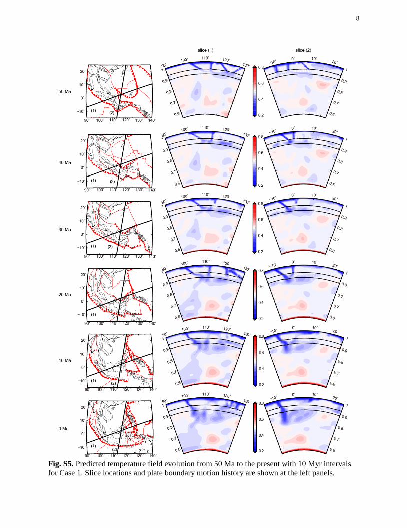
Fig. S5. Predicted temperature field evolution from 50 Ma to the present with 10 Myr intervals

for Case 1. Slice locations and plate boundary motion history are shown at the left panels.

9

Fig. S6. Comparison between observed [Heidbach et al., 2010] regional principal stress direction

(green lines) and predicted present-day mantle flow-induced principal stress direction for case 1

at 10 km depth (yellow).

Reference and Notes:

Becker, T. W., and L. Boschi (2002), A comparison of tomographic and geodynamic mantle models, Geochem.

Geophys. Geosyst., 3(1), 10.129/2001GC000168.

Doust, H., and H. S. Sumner (2007), Petroleum systems in rift basins–a collective approach in Southeast Asian

basins, Pet. Geosci., 13(2), 127-144.

Gudmundsson, Ó., and M. Sambridge (1998), A regionalized upper mantle (RUM) seismic model, J. Geophys. Res.,

103(B4), 7121-7136.

Heidbach, O., M. Tingay, A. Barth, J. Reinecker, D. Kurfeß, and B. Müller (2010), Global crustal stress pattern

based on the World Stress Map database release 2008, Tectonophysics, 482(1), 3-15.

Li, C., R. D. van der Hilst, E. R. Engdahl, and S. Burdick (2008), A new global model for P wave speed variations

in Earth's mantle, Geochem. Geophys. Geosyst., 9(5), Q05018, doi:05010.01029/02007GC001806.

Madon, M. B., and A. Watts (1998), Gravity anomalies, subsidence history and the tectonic evolution of the Malay

and Penyu Basins (offshore Peninsular Malaysia), Basin Res., 10(4), 375-392.

Pigott, J. D., and N. Sattayarak (1993), Aspects of sedimentary basin evolution assessed through tectonic subsidence

analysis. Example: northern Gulf of Thailand, J. Southeast. Asian Earth Sci., 8(1), 407-420.

Ritsema, J., A. Deuss, H. Van Heijst, and J. Woodhouse (2011), S40RTS: a degree-40 shear-velocity model for the

mantle from new Rayleigh wave dispersion, teleseismic traveltime and normal-mode splitting function

measurements, Geophys. J. Int., 184(3), 1223-1236.