supplementary information - images.nature.com · basins traceable (m. moros unpublished loss on...

SUPPLEMENTARY INFORMATIONDOI: 10.1038/NCLIMATE1595

NATURE CLIMATE CHANGE | www.nature.com/natureclimatechange 1

SUPPLEMENTARY INFORMATION

page 1 of 21

Impact of climate change on the Baltic Sea ecosystem over the last 1000 years

Karoline Kabel, Matthias Moros, Christian Porsche, Thomas Neumann, Florian Adolphi, Thorbjørn Joest Andersen, Herbert Siegel, Monika Gerth, Thomas Leipe, Eystein Jansen, Jaap S. Sinninghe Damsté

Contents

Part A: Proxy data page 2

A1. Material and analytical methods page 2

A2. Age model page 4

A3. TEX86 calibration for the Baltic Sea and application page 7

A4. Summer SSTs and cyanobacteria blooms during the last 40 years page 9

A5. Biogenic silica page 11

A6. References page 12

Part B: Modelling approach page 15

B1. Model description and validation page 15

B2. LIA Scenario model adaptation with pristine nutrient loads page 17

B3. LIA scenario with modern nutrient loads page 19

B4. LIA scenario with wind speed variations page 19

B5. References page 20

Impact of climate change on the Baltic Sea ecosystem over the past 1,000 years

© 2012 Macmillan Publishers Limited. All rights reserved.


page 2 of 21

Part A: Proxy data A1. Material and analytical methods

Sampling and sample preparation: For this study sediment cores were taken during

several cruises using a multi corer and a gravity corer (station ID, location, cruises etc. see

Table S1). Most of the multi-cores were sampled by cutting the core from top to bottom in 0.5

or 1 cm slices. The gravity cores and some multi cores were carefully cut into halves before

sampling thus allowing more precise sampling and photographic documentation. The

samples were freeze-dried and grounded for further analyses.

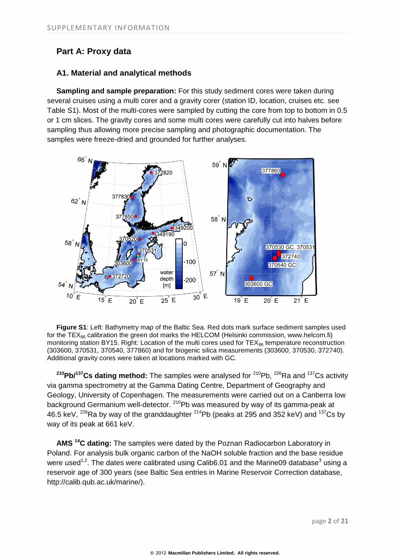
Figure S1: Left: Bathymetry map of the Baltic Sea. Red dots mark surface sediment samples used for the TEX86 calibration the green dot marks the HELCOM (Helsinki commission, www.helcom.fi) monitoring station BY15. Right: Location of the multi cores used for TEX86 temperature reconstruction (303600, 370531, 370540, 377860) and for biogenic silica measurements (303600, 370530, 372740). Additional gravity cores were taken at locations marked with GC.

210Pb/137Cs dating method: The samples were analysed for 210Pb, 226Ra and 137Cs activity

via gamma spectrometry at the Gamma Dating Centre, Department of Geography and

Geology, University of Copenhagen. The measurements were carried out on a Canberra low

background Germanium well-detector. 210Pb was measured by way of its gamma-peak at

46.5 keV, 226Ra by way of the granddaughter 214Pb (peaks at 295 and 352 keV) and 137Cs by

way of its peak at 661 keV.

AMS 14C dating: The samples were dated by the Poznan Radiocarbon Laboratory in

Poland. For analysis bulk organic carbon of the NaOH soluble fraction and the base residue

were used1,2. The dates were calibrated using Calib6.01 and the Marine09 database3 using a

reservoir age of 300 years (see Baltic Sea entries in Marine Reservoir Correction database,

http://calib.qub.ac.uk/marine/).



page 3 of 21

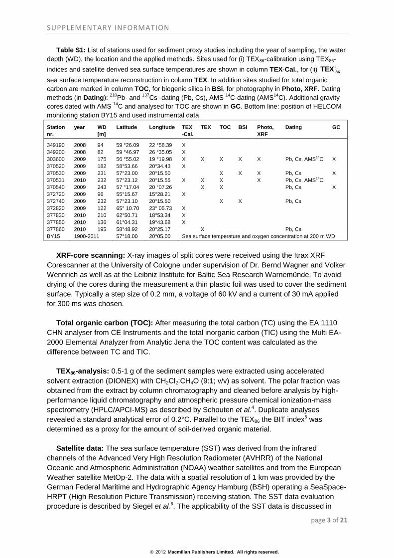
Table S1: List of stations used for sediment proxy studies including the year of sampling, the water

depth (WD), the location and the applied methods. Sites used for (i) TEX86-calibration using TEX86-

indices and satellite derived sea surface temperatures are shown in column TEX-Cal., for (ii) L86TEX

sea surface temperature reconstruction in column TEX. In addition sites studied for total organic

carbon are marked in column TOC, for biogenic silica in BSi, for photography in Photo, XRF. Dating

methods (in Dating): 210

Pb- and 137

Cs -dating (Pb, Cs), AMS 14

C-dating (AMS14

C). Additional gravity

cores dated with AMS 14

C and analysed for TOC are shown in GC. Bottom line: position of HELCOM

monitoring station BY15 and used instrumental data.

Station nr.

year WD [m]

Latitude Longitude TEX-Cal.

TEX TOC BSi Photo, XRF

Dating GC

349190 2008 94 59 °26.09 22 °58.39 X

349200 2008 82 59 °46.97 26 °35.05 X

303600 2009 175 56 °55.02 19 °19.98 X X X X X Pb, Cs, AMS14

C X

370520 2009 182 58°53.66 20°34.43 X

370530 2009 231 57°23.00 20°15.50 X X X Pb, Cs X

370531 2010 232 57°23.12 20°15.55 X X X X Pb, Cs, AMS14

C

370540 2009 243 57 °17.04 20 °07.26 X X Pb, Cs X

372720 2009 96 55°15.67 15°28.21 X

372740 2009 232 57°23.10 20°15.50 X X Pb, Cs

372820 2009 122 65° 10.70 23° 05.73 X

377830 2010 210 62°50.71 18°53.34 X

377850 2010 136 61°04.31 19°43.68 X

377860 2010 195 58°48.92 20°25.17 X Pb, Cs

BY15 1900-2011 57°18.00 20°05.00 Sea surface temperature and oxygen concentration at 200 m WD

XRF-core scanning: X-ray images of split cores were received using the Itrax XRF

Corescanner at the University of Cologne under supervision of Dr. Bernd Wagner and Volker

Wennrich as well as at the Leibniz Institute for Baltic Sea Research Warnemünde. To avoid

drying of the cores during the measurement a thin plastic foil was used to cover the sediment

surface. Typically a step size of 0.2 mm, a voltage of 60 kV and a current of 30 mA applied

for 300 ms was chosen.

Total organic carbon (TOC): After measuring the total carbon (TC) using the EA 1110

CHN analyser from CE Instruments and the total inorganic carbon (TIC) using the Multi EA-

2000 Elemental Analyzer from Analytic Jena the TOC content was calculated as the

difference between TC and TIC.

TEX86-analysis: 0.5-1 g of the sediment samples were extracted using accelerated

solvent extraction (DIONEX) with CH2Cl2:CH4O (9:1; v/v) as solvent. The polar fraction was

obtained from the extract by column chromatography and cleaned before analysis by high-

performance liquid chromatography and atmospheric pressure chemical ionization-mass

spectrometry (HPLC/APCI-MS) as described by Schouten et al.4. Duplicate analyses

revealed a standard analytical error of 0.2°C. Parallel to the TEX86 the BIT index5 was

determined as a proxy for the amount of soil-derived organic material.

Satellite data: The sea surface temperature (SST) was derived from the infrared

channels of the Advanced Very High Resolution Radiometer (AVHRR) of the National

Oceanic and Atmospheric Administration (NOAA) weather satellites and from the European

Weather satellite MetOp-2. The data with a spatial resolution of 1 km was provided by the

German Federal Maritime and Hydrographic Agency Hamburg (BSH) operating a SeaSpace-

HRPT (High Resolution Picture Transmission) receiving station. The SST data evaluation

procedure is described by Siegel et al.6. The applicability of the SST data is discussed in



page 4 of 21

Siegel et al.7 and systematic studies on seasonal and inter-annual variations in SST are

published by Siegel et al.6,8. The yearly development of SST in the Baltic is described in the

German assessment of the state of the Baltic Sea9 and in the HELCOM indicator fact

sheets10.

Ocean colour satellite data from SeaWiFS (Sea-viewing Wide Field-of-view Sensor) and

MODIS (Moderate Resolution Imaging Spectroradiometer) is implemented to study the inter-

annual differences in the development of cyanobacteria in summer. The chlorophyll

concentration of the summer months was derived using algorithms, based on channels 4 and

5. SeaWiFS considers the scattering properties7. In summer the light scattering of the water

is dominated by cyanobacteria. For the validation of the inter-annual variation of the

SeaWiFS derived chlorophyll pattern a SeaWiFS/MODIS derived Level 3 product of the

reflectance at 550 nm was applied. This parameter represents the spectral maximum of

reflectance in the Baltic Sea and variations are produced by backscattering of particle, i.e.

cyanobacteria in summer. The spatial resolutions of the data were different: SeaWiFS

derived chlorophyll: 1 km; reflectance at 550 nm from SeaWiFS and MODIS 9 and 4 km,

respectively.

Time series of instrumental SST: The instrumental SST data for the HELCOM

monitoring station BY15 was retrieved from the ICES oceanographic database11 for the time

period 1969-2011. A 5-year moving average was calculated for August-September

measurements for the period 1971-2008 using only years where sufficient data was

available. The data before 1969 was retrieved from the Baltic Environmental Database

(BED)12 and average August-September SST values were calculated for years where

sufficient data was available.

Biogenic silica (BSi): 0.1 g of sediment was used to extract BSi with 100 ml 1 M NaOH

for 40 min. at 85°C. The extract was decanted after centrifugation and BSi was detected

using the Molybdate-blue method, for the composition of specific reagents see Müller &

Schneider13. 6 ml of molybdate reagent was added to 1 ml of extract and mixed for 5 min and

then 6 ml of oxalic acid reagent and 6 ml of ascorbic acid reagent were added and mixed for

15 min. BSi was detected with a SPEKOL 1100 photometer from “Analytik Jena” measuring

the absorbance at a wavelength of 660 nm.

A2. Age model

Modern Warm Period / Little Ice Age: The multi cores showed a clear tendency for

exponential decline of unsupported 210Pb with depth (typically back to around 1880-1900)

and no signs of mixing (bioturbation) of the top laminated section. The chronologies were

supported by the 1986 peak in 137Cs (Chernobyl accident) but the peak was often less well-

defined due to continued supply of the isotope to the Baltic Sea after 1986 (Figure S2). In

addition, a basin-wide traceable soft, water-rich diatom layer dilutes the 137Cs signal at a

certain depth interval (Figure S2). This marked layer was deposited during massive diatom

blooms between 1988 and 199014. The diatom layer, therefore, provides an additional datum

level to our age models. In cores from deeper basin sites (high sedimentation rates) high-

resolution 137Cs measurements did also pick up the atmospheric 1963 peak in 137Cs due to

nuclear weapons testing. AMS 14C of bulk organic carbon and of two organic carbon fractions



page 5 of 21

Figure S2: X-radiographs,

137Cs and organic carbon profiles of multi cores taken in the Gotland

basin at different water depth. Stratigraphic marker horizons are indicated and dating methods used

for certain depths/time intervals (see box). Please note the appearance of a very water rich diatom

layer (X-radiograph) which was deposited during massive diatom blooms 1988-1990 and which dilutes

the 137

Cs signal.

(NaOH soluble fraction and base residue), respectively, agree with the 210Pb/137Cs age model

where bomb/modern radiocarbon was measured in the organic carbon rich laminated

sediments deposited after 1963 (Figure S2). Additional proof of the age model quality is

provided by traceable manganese-carbonate layers (Figure S2). The age model was



page 6 of 21

extrapolated to the Little Ice Age (LIA, back to 1850). The term LIA is used in the broader

sense from ~1350-1850 here.

Medieval Climatic Anomaly: The widely recognized and over all the deeper Baltic Sea

basins traceable (M. Moros unpublished loss on ignition and organic carbon data) second

organic carbon-rich laminated section (Figure S2, S3 and 2 main text) was deposited during

the Medieval Climatic Anomaly15,16,17,18 (MCA). The organic carbon maximum of these

laminated sediments (marked organic carbon spike in multi and gravity cores) were dated to

c. 1240 ± 30 14C years in cores from the central Gotland basin (Table S2, Figure S3). This is

clearly in the time span of the MCA: calibrated age is A.D. 1004-1154 one sigma range using

a reservoir age of 300 years (see Baltic Sea entries in Marine Reservoir Correction

database, http://calib.qub.ac.uk/marine/). A rather low reservoir age is very likely as the high

organic carbon content is due to massive cyanobacteria blooms at the sea surface during

Figure S3: Total organic carbon (TOC) content of gravity cores from sites with different

sedimentation rates in the Gotland Basin (see Figure1). The TOC spike represents the Medieval

Climate Anomaly (MCA) (laminated) as shown by AMS 14

C-dating (marked by a star) and is followed

by lower values during the Little Ice Age (LIA) (homogenous). Due to the sampling technique the

sediment surface including the Modern Warm Period is missing.

Table S2: AMS

14C dates of the organic carbon maximum of the laminated section deposited

during the Medieval Climatic Anomaly from multi cores (MUC) and gravity cores (GC) from the

Gotland Basin.

Lab. code Core ID depth

(cm) Raw AMS 14C date (BP 1950) Material dated

Poz-37518 370530GC 33.5 1260 ± 30 bulk, NaOH

Poz-20706

Poz-20734

280290-3MUC 49 1235 ± 30

1255 ± 30

bulk, NaOH

bulk, residue

Poz-20735

Poz-20792

303600GC 17 1230 ± 30

1275 ± 30

bulk, NaOH

bulk, residue

Poz-31577 370540GC 43.5 1260 ± 30 bulk

Poz-38099 303600MUC 44.5 1225 ± 30 bulk



page 7 of 21

Modern Warm Period (MoWP) and MCA19 (see main text). The fine lamination results from

calm deposition under anoxic conditions and weak input of old organic carbon at the studied

sites which is also evidenced by the modern ages for the recent/sub-recent sediments from

the same sites (Figure S2). In addition, atmospheric lead pollution data evidence an age of

A.D. 1200 for this laminated section18.

A3. TEX86 calibration for the Baltic Sea and application

Comparison of sediment surface TEX-indices with satellite derived SSTs: The

TEX86-index reflects temperature-induced changes in the composition of membrane lipids of

Thaumarchaeota20, former mesophilic Crenarchaeota21. Correlation of the index with sea

surface temperature (SST) has been shown for worldwide data sets22 as well as for regional

data sets23,24. Here we establish a local calibration, which – for the first time – allows past

SST reconstructions for the Baltic Sea. Established methods for marine temperature

reconstructions like Mg/Ca ratio of planktonic foraminifera and Uk’37 of alkenones

(haptophytes) do not work because the specific organisms are absent (i.e. foraminifers) in

the brackish Baltic Sea or their distribution (alkenones) is too much influenced by brackish

haptophytes that have an unknown SST-Uk’37 relationship.

Nine surface sediment samples (0-1 cm) from the Baltic Sea (Figure S1, Table S1) were

analyzed for TEX86 and the data was compared with satellite derived SST data. The sites

were carefully chosen in order to obtain high-quality surface samples (i.e. of modern age)

and are spread over the whole Baltic Sea to cover the largest temperature range possible.

The samples were checked for soil organic matter input (which may influence TEX86 ) using

Table S3: Satellite derived monthly averaged sea surface temperatures (SST) for the last six years

prior to year of sediment sampling at the nine stations. TEX-indices were calculated: TEX86 (Ref. 20),

H86TEX and L

86TEX (Ref. 22). In addition, the determination coefficient, R

2, of linear regression of TEX-

indices with monthly as well as July-to-October satellite derived SST is shown.

Monthly mean SSTs [°C] of the stations: Determination Coefficient:

303600 349190 349200 370520 370531 372720 372820 377830 377850

R2 TEX86

R2 L86TEX

R2 H86TEX

May 7.5 5.9 6.4 6.7 7.2 8.3 1.5 4.5 3.5 0.51 0.71 0.53

Jun 13.1 11.9 12.9 12.1 13.0 13.5 8.2 10.8 10.0 0.51 0.74 0.58

Jul 17.7 18.1 18.5 17.5 18.6 17.9 15.0 15.7 16.3 0.75 0.87 0.76

Aug 18.9 19.1 19.6 18.6 19.0 18.5 16.2 16.5 17.4 0.81 0.84 0.81

Sep 15.9 15.9 15.6 15.0 15.7 16.2 11.7 13.0 13.4 0.71 0.81 0.71

Oct 12.3 11.8 11.3 12.4 12.6 13.0 8.3 8.6 9.7 0.61 0.86 0.62

Nov 8.8 7.3 6.4 8.5 8.8 9.2 4.9 5.3 5.9 0.44 0.75 0.46

Jul-Oct 16.2 16.2 16.2 15.9 16.5 16.0 12.8 13.4 14.2 0.89

TEX-indices of sediment surface samples of the stations:

Tex86 0.42 0.43 0.42 0.41 0.42 0.38 0.35 0.35 0.34 L86TEX

-0.59 -0.62 -0.61 -0.61 -0.58 -0.62 -0.69 -0.69 -0.64

H86TEX

-0.38 -0.36 -0.38 -0.39 -0.38 -0.42 -0.45 -0.46 -0.47



page 8 of 21

Figure S4: Correlation of L86TEX with July to October satellite-derived sea surface temperatures

using the bootstrapping method including the 95% confidence interval. The blue shaded area

represents the range of L86TEX values from the central Baltic for the Little Ice Age (LIA).

the BIT index. BIT values < 0.1 indicate almost no soil organic matter input25 at most sites,

the exception being site 377850 in the southern Bothnian Sea. At site 377850 we found a

BIT index of 0.3 which indicates some terrestrial influence but with no apparent influence on

the calibration. We chose satellite derived SST data for the calibration due to its higher

temporal resolution compared to in-situ measurements. For the satellite derived SSTs we

used monthly averaged values of the last six years prior to the year of sediment sampling.

Only the ice-free months (May-November) are used as winter SSTs are biased by ice cover.

The R² value of the three different TEX indices TEX86 (Ref.4), H86TEX and L

86TEX (Ref. 22)

were compared to identify the index with the best correlation to monthly SST (Table S3). As

expected for the temperate Baltic Sea the highest correlation coefficient was reached by L86TEX , with the best single month correlation in July with R2=0.87. A combination of several

months (July to October) was found to improve the correlation for L86TEX (R2=0.89, Figure

S4). We applied the bootstrapping method on these July-October SSTs to check the quality

of and to improve the regression SST model. The bootstrapping method is based on re-

sampling of a data set and allows the assessment of quantities associated with the sampling

distribution. The 95% confidence interval for the regression model is shown in Figure S4.

Please note that for the TEX86 values during the LIA the uncertainty of the estimated SST is

max +-0.5°C based on the 95% confidence interval.

Comparison of subsurface sediment derived SSTs with instrumental data: The new

calibration was applied on four multi cores with sound chronological control (one from the

Northern Gotland Basin and three from the Eastern Gotland Basin, Figure S5). The BIT index

at all sites is less than 0.1 indicating no soil-derived organic matter bias. All cores show the

same temperature pattern over the past 170 years, a marked temperature increase of about

2°C (Figure S5).

A comparison of instrumental and proxy down core SST data is shown in Figure S5. The

mean L86TEX -SST (TEX-mean) is used calculated as the mean of annual resolved splines for

each of the four cores studied. The instrumental data from central Gotland Basin shown is a



page 9 of 21

Figure S5: To the left: comparison of TEX86-temperature reconstructions of the past 170 years of

the surface sediment cores 370531, 370540N-B, 303600N and 377860-1 from the central Baltic. To

the right: TEX86-temperature reconstruction ensemble/core mean (TEX-mean) with TEX-mean ±

standard deviation (Std) and 5-year moving average instrumental SSTs for August to September since

1971 at HELCOM monitoring station BY15 (Ref. 11), measurements before 1971 (single dots) are

presented for years when August and September SST data are available12

. The trends in instrumental

and proxy TEX86 SSTs are indicated by straight lines. A vertical grey bar marks the suggested

minimum summer SST needed to enable cyanobacteria blooms in the Baltic Sea27, 28

. Note that during

the cold summers in the 1980s (arrow) cyanobacteria blooms did not occur26

.

5-year running average of mean SSTs (0-5 m water depths) from1971-2008. Since the

sampling resolution for October is rather poor only August to September mean SST values

were used. Before 1971 only for a few years SST measurements are available for August

and September (Figure S5).

The instrumental and proxy SST data compare well for the time period 1971 to 2008. In

particular, the cold years of the late 1980s, during which no cyanobacteria blooms were

observed26 in the Baltic Sea, are reproduced well. Although the reliability of the longer-term

warming trend in the instrumental SST data is low due to scarce data available before 1969,

the trend fits to the SST increase reconstructed by our proxy data since the LIA. Noteworthy

is the strong inter-annual summer SST variability evident from the instrumental data of the

last 40 years (see Figure S7). However summer SSTs above 16°C the threshold for

cyanobacteria blooms27, 28 were not reached during the LIA.

In addition, further instrumental temperature measurements of sea water beginning 1900

(discontinuous) at the Gotland basin monitoring station BY15 (Ref. 29) display a similar

temperature rise at 80 m water depth, as well as air temperature records (Tallinn30,

Stockholm31, 32) and tree ring data33. The similar temperature range in other instrumental

data/ reconstructions supports our reconstruction.

Very little is known about Thaumarchaeota in the Baltic Sea regarding their seasonal

occurrence and their preferred living depth in the water column. Their presence at the



page 10 of 21

chemocline at about 80m water depth has been reported34, but it remains impossible

presently to consider ecological factors in the Baltic Sea TEX86 calibration.

A4. Summer SSTs and cyanobacteria blooms during the last 40 years

Monthly mean satellite derived SST, chlorophyll-a (Chl-a), and reflectance at 550 nm for

the summer months were used to investigate inter-annual variations in the intensity of

cyanobacteria development and SST, which are also strongly related to wind mixing. During

low wind conditions a diurnal thermocline is established, which supports a faster heating, and

due to the buoyancy the cyanobacteria flow up to the surface and to the light. This intensifies

the cyanobacteria growth and the development of surface scum and increases the spectral

reflectance of the water. Wind mixing distributes the incoming heat flux and the

cyanobacteria in the top layer and, consequently, reduces the surface temperature and

cyanobacteria abundance. Examples from the period 1998-2001 are presented for the month July in Figure S6. SST

in the Baltic Sea was characterized by colder summers in 1998 and 2000 and warmer in

Figure S6: Monthly mean satellite derived SST, Chl-a and reflectance at 550 nm for the summer

month July of period 1998 to 2001 representing the inter-annual differences in the surface

temperature and in the development of cyanobacteria.



page 11 of 21

1999 and 2001. Clear inter-annual differences occurred in the satellite derived Chl-a

concentration and in the reflectance at 550 nm. Both parameters consider particle scattering

dominated by cyanobacteria in summer in the Baltic Sea. More intense cyanobacteria

blooms developed in the warmer years 1999 and 2001 (Ref. 35). These inter-annual

variations are in a good agreement with the results published by Kahru et al.36. Monthly mean

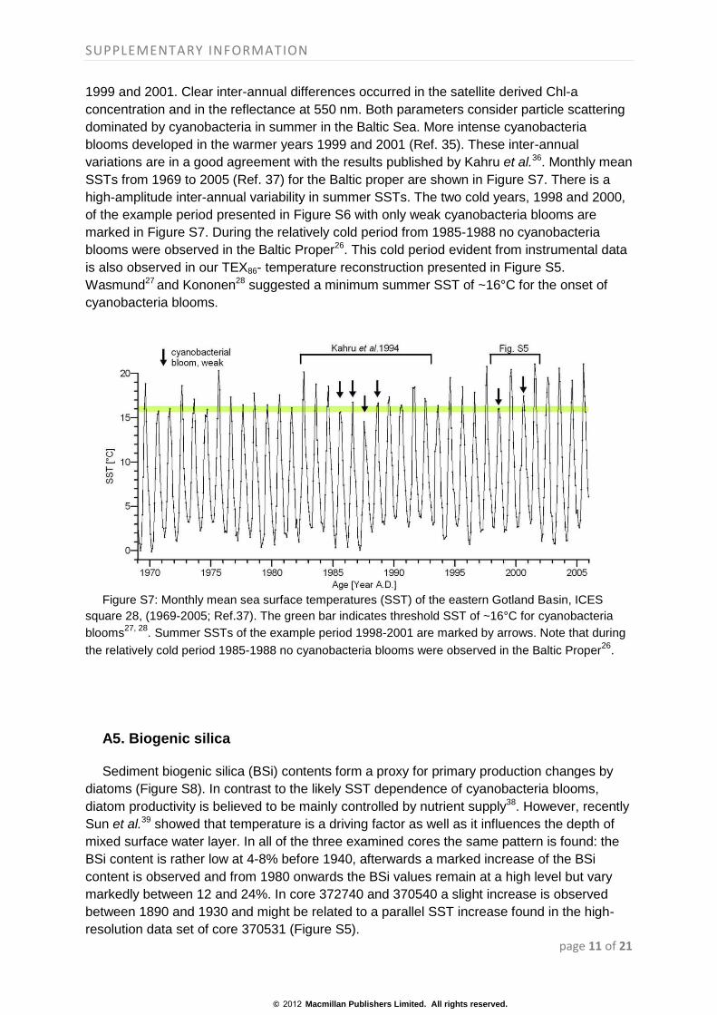
SSTs from 1969 to 2005 (Ref. 37) for the Baltic proper are shown in Figure S7. There is a

high-amplitude inter-annual variability in summer SSTs. The two cold years, 1998 and 2000,

of the example period presented in Figure S6 with only weak cyanobacteria blooms are

marked in Figure S7. During the relatively cold period from 1985-1988 no cyanobacteria

blooms were observed in the Baltic Proper26. This cold period evident from instrumental data

is also observed in our TEX86- temperature reconstruction presented in Figure S5.

Wasmund27 and Kononen28 suggested a minimum summer SST of ~16°C for the onset of

cyanobacteria blooms.

Figure S7: Monthly mean sea surface temperatures (SST) of the eastern Gotland Basin, ICES

square 28, (1969-2005; Ref.37). The green bar indicates threshold SST of ~16°C for cyanobacteria

blooms27, 28

. Summer SSTs of the example period 1998-2001 are marked by arrows. Note that during

the relatively cold period 1985-1988 no cyanobacteria blooms were observed in the Baltic Proper26

.

A5. Biogenic silica

Sediment biogenic silica (BSi) contents form a proxy for primary production changes by

diatoms (Figure S8). In contrast to the likely SST dependence of cyanobacteria blooms,

diatom productivity is believed to be mainly controlled by nutrient supply38. However, recently

Sun et al.39 showed that temperature is a driving factor as well as it influences the depth of

mixed surface water layer. In all of the three examined cores the same pattern is found: the

BSi content is rather low at 4-8% before 1940, afterwards a marked increase of the BSi

content is observed and from 1980 onwards the BSi values remain at a high level but vary

markedly between 12 and 24%. In core 372740 and 370540 a slight increase is observed

between 1890 and 1930 and might be related to a parallel SST increase found in the high-

resolution data set of core 370531 (Figure S5).



page 12 of 21

Figure S8: Biogenic silica (% of dry weight) profiles of three cores from the Eastern Gotland Basin

versus age. Please note the marked increase after 1940.

A6. References

1. Kigoshi, K., Suzuki, N. & Shiraki, M. Soil dating by fractional extraction of humic acid.

Radiocarbon. 22, 853–857 (1980).

2. Brock, F., Higham, T., Ditchfield, P. & Bronck Ramsey, C. Current pretreatment

methods for AMS radiocarbon dating at Oxford Radiocarbon Accelerator Unit

(ORAU). Radiocarbon 52, 103–112 (2010).

3. Stuiver, M. & Reimer, P. J. Extended 14C database and revised CALIB radiocarbon

calibration program. Radiocarbon 35, 215–230 (1993).

4. Schouten, S., Huguet, C., Hopmans, E. C., Kienhuis, M. V. M. & Sinninghe Damsté,

J. S. Analtytical Methodology for TEX86 Paleothermometry by High-Performance

Liquid Chromatography/Atmospheric Pressure Chemical Ionization-Mass

Spectrometry. Anal. Chem. 79, 2940–2944 (2007).

5. Hopmans, E. C., Weijers, W. H., Schefuß, E., Herfort, L., Sinninghe Damsté, J. S. &

Schouten, S. A novel proxy for terrestrial organic matter in sediments based on

branched and isoprenoid tetraether lipids. Earth Planet. Sc. Lett. 224, 107–116

(2004). 6. Siegel H., Gerth M. & Tschersich G. in: State And Evolution Of The Baltic Sea, 1952-

2005. A Detailed 50-year Survey Of Meteorology And Climate, Physics, Chemistry,

Biology, And Marine Environment. (eds Feistel R., G. Nausch & Wasmund N.) Ch. 9

(Wiley, 2008).

7. Siegel, H., Gerth, M. & Gade, M. Remote Sensing Of The Pomeranian Bight By

Different Optical And Microwave Sensors During The Oder Flood In August 1997.

IGARSS '99: proceedings IEEE International, 308–310 (1999).

8. Siegel, H., Gerth, M. & Tschersich, G. Sea surface temperature development of the

Baltic Sea in the period 1990-2004. Oceanologia 48, 119–131 (2006).



page 13 of 21

9. Nausch, G., Feistel R., Umlauf, L., Mohrholz, V. & Siegel, H. Hydrographisch-

chemische Zustandseinschätzung der Ostsee 2010. Marine Science Reports 84, Warnemünde: Leibniz-Institut for Baltic Sea Research. (2011).

10. Siegel, H. & Gerth, M. Development of Sea Surface Temperature in the Baltic Sea in

2009. HELCOM Indicator Report (2010). 11. ICES Oceanographic Database http://ocean.ices.dk/ (2012). 12. Baltic Nest Institute Baltic Environmental Database (BED) http://nest.su.se/bed/

(2011). 13. Müller. J. P. & Schneider, R. An automated leaching method for the determination of

opal in sediments and particulate organic matter. Deep-Sea Res. Pt. I 40, 425–444

(1993). 14. Wasmund, N., Polehne, F., Postel, L., Siegel, H. & Zettler, M. L. Biologische

Zustandseinschätzung der Ostsee im Jahr 2004. Marine Science Reports 84, Warnemünde: Leibniz-Institut for Baltic Sea Research. (2005).

15. Harff, J. et al. in The Baltic Sea Basin (eds Harff, J., Björk, S. & Hoth, P.) Ch. 5

(Springer, 2011).

16. Zillén L., Conley D. J., Andrén T., Andrén E. & Björck S. Past occurrences of hypoxia

in the Baltic Sea and the role of climate variability, environmental change and human

impact. Earth-Sci. Rev. 91, 77–92 (2008).

17. Andrén, E. & Andrén, T. Holocene history of the Baltic Sea as abackground for

assessing records of human impact in the sediments of the Gotland Basin. Holocene

10, 687–702 (2000).

18. Lougheed, B. C. et al. Using an independent geochronology based on

palaeomagnetic secular variation (PSV) and atmospheric Pb deposition to date Baltic

Sea sediments and infer 14C reservoir age. Quat. Sci. Rev. 42, 43–58 (2012).

19. Kowalewska, G. Algal pigments in Baltic sediments as markers of ecosystem and

climate changes. Clim. Res. 88, 89–96 (2001).

20. Schouten, S., Hopmans, E. C., Schefuß, E. & Sinninghe Damsté, J. S. Distributional

variations in marine crenarchaeotal membrane lipids: A new organic proxy for

reconstructing ancient sea water temperatures? Earth Planet. Sci. Lett. 204, 265–

274 (2002).

21. Brochier-Armanet, C., Boussau, B., Gribaldo, S. & Forterre, P. Mesophilic

crenarchaeota: proposal for a third archaeal phylum, the Thaumarchaeota. Nature 6, 245–252 (2008).

22. Kim, J.-H. et al. New indices and calibrations derived from the distribution of

crenarchaeal isoprenoid tetraether lipids: implications for past sea surface

temperature reconstructions. Geochim. Cosmochim. Acta 74, 4639–4654 (2010).

23. Leider, A., Hinrichs, K.-U., Mollenhauer, G. & Versteegh, G. J. M. Core-top

calibration of the lipid-based UK′37 and TEX86 temperature proxies on the southern

Italian shelf (SW Adriatic Sea, Gulf of Taranto), Earth Planet. Sc. Lett. 300, 112–124

(2010).

24. Shevenell A. E., Ingalls A. E., Domack E. W. & Kelly, C. Holocene Southern Ocean

surface temperature variability west of the Antarctic Peninsula. Nature 470, 250–254

(2011) 25. Weijers, J. W. H., Schouten, S., Spaargaren, O. C. & Sinninghe Damsté, J. S.

Occurrence and distribution of tetraether membrane lipids in soils: Implications for

the use of the TEX86 proxy and the BIT index. Org. Geochem. 37, 1680–1693

(2006).


http://ocean.ices.dk/

http://nest.su.se/bed/


page 14 of 21

26. Kahru, M., Horstmann, U. & Rud, O. Statellite Detection of Increased Cyanobacteria

Blooms in the Baltic Sea: Natural Fluctuation or Ecosystem Change? Ambio 23, 469–472 (1994).

27. Wasmund, N. Occurrence of Cyanobacteria Blooms in the Baltic Sea in Relation to

Environmental Conditions. Int. Rev. Ges. Hydrobiol. 82, 169–184 (1997).

28. Kononen, K. Dynamics of the toxic cyanobacteria blooms in the Baltic Sea. Finn.

Mar. Research 261, 3–36 (1992).

29. Fonselius, S. & Valderrama, J. One hundred years of hydrographic measurements in

the Baltic Sea. J. Sea Res. 49, 229–241 (2003).

30. Tarand, A. & Nordli, P. Ø. The Tallinn temperature series reconstructed back half a

millennium by use of proxy data. Clim. Change 48, 189–99 (2001).

31. Moberg, A., Bergström, H., Ruiz Krigsman, J. & Svanered, O. Daily air temperature

and pressure series for Stockholm (1756–1998) Clim. Change 53, 171–212 (2002).

32. Leijonhufvud L., Wilson R. & Moberg A. Documentary data provide evidence of

Stockholm average winter to spring temperatures in the eighteenth and nineteenth

centuries. The Holocene 18, 333–343 (2008).

33. Esper, J., Büntgen, U., Timonen, M. & Frank, D. C. Variability and extremes of

northern Scandinavian summer temperatures over the past two millennia. Global

Planet. Change 88–99, 1–9 (2012).

34. Labrenz, M., Jost, G. & Jürgens, K. Distribution of abundant prokaryotic organisms in

the water column of the central Baltic Sea with an oxic-anoxic interface. Aquat.

Microb. Ecol. 46, 177–190 (2007).

35. Siegel, H. & Gerth, M. In: Remote Sensing of European Seas. (eds Barale, V., Gade,

M.) 91–102 (Springer, 2008). 36. Kahru, M., Savchuk, O. P. & Elmgren, R. Satellite measurements of cyanobacteria

bloom frequency in the Baltic Sea: interannual and spatial variability. Mar. Ecol.

Prog. 343, 15–23 (2007).

37. Lehmann, A. & Hinrichsen, H.-H. Trends of temperature in the Baltic Sea for the

period 1969-2005 and long-term variability in winter water mass formation. BALTEX

Newsletter 10, 7–10 (2007).

38. Weckström, K., Korhola, A. & Weckström, J. Impacts of Eutrophication on Diatom

Life Forms and Species Richness in Coastal Waters of the Baltic Sea. Ambio 36, 155-160 (2007).

39. Sun, X. et al. Climate dependent diatom production is preserved in biogenic Si

isotope signatures. Biogeosci. 8, 3491–3499 (2011).



page 15 of 21

Part B: Modelling approach

B1. Model description and validation

The model used for the simulation of the Modern Warm Period (MoWP) and the Little Ice

Age (LIA) is composed of a three dimensional circulation model with an integrated biological

geochemical ecosystem model which is based on a nine component model, called Ecological

Regional Ocean Model (ERGOM)40,41. The physical part of the circulation model is based on

the Modular Ocean Model (MOM) version 3.1 (Ref. 42). The grid structure of the used model

has 222 longitudinal, 240 latitudinal, and 77 depth levels. Whereas the longitudinal resolution

is 0.1 degree and the latitudinal resolution is 0.05 degree that corresponds to about three

nautical miles. The vertical resolution is about 1.5 m for the upper 28 m and increases with

depth to 5 m in more than 100 m depth. So the model covers the Baltic Sea with a total area

of 0.443E12 m2 and a total volume of 0.244E14 m3. At the western border of the Skagerrak an

open boundary condition with prescribed mean sea level, salinity, temperature, and

biogeochemical variables was applied43. Furthermore, the inflow of riverine freshwater loaded

with nutrients (ammonium, nitrate and phosphate) was included for the runoff of the 20

Figure S9: Taylor diagram, which shows differences in chosen variables of the model and

observations. The circular arc around the point of origin prescribes the normalized standard deviation,

whereas the observational data set are represented by a dot on the abscissa at normalized standard

deviation of 1.0. The grey circles around this reference point show the deviation of the centred root

mean square (cRMS) and the dotted lines refer to the rank correlation coefficient by Spearman. The

shapes of the points represent the different periods and the colours correspond to the different

variables (c(DIN): Dissolved Inorganic Nitrogen, σ(O2): oxygen concentration, c(PO43-

). phosphate

concentration, S: salinity, T: temperature).



page 16 of 21

largest rivers along the Baltic Sea coastline. Ice cover, thickness and extent were simulated

by a thermodynamic ice model44. Finally the model was driven with realistic atmospheric

forcing including atmospheric deposition of nutrients as well. The data for these realistic

forcing was derived from the ERA-40 project45. With these forcing data it was possible to

simulate the MoWP scenario for 47 years from 1961 to 2007 which serves as the reference.

Because the model ecosystem has to adapt to the external conditions and so to avoid a spin

off effect new initial conditions were calculated from the last time step of the first model

simulation. Furthermore the model was started again for another two times with different

initial conditions taken from the second model run. Finally there are three simulations which

do not have a strong spin off effect and which vary only in their initial conditions. The

ensemble results of these simulations with their realistic forcing are the basis to validate the

model by comparing it with instrumental data. This will provide confidence to the used model.

The validation of the model was carried out for selected variables which are temperature,

salinity, concentration of oxygen, dissolved inorganic nitrogen (ammonium and nitrate), and

phosphate. For this purpose the instrumental values of chosen variables were averaged over

the month in every accordant model grid cell. The distribution of the variables was checked

to conclude the next steps of statistical analyses which should provide information about the

confidence of the model. After a first descriptive statistical analysis of the observed and

modelled data, both data sets are not normally distributed. Figure S9 summarizes some

important statistical values in form of a Taylor diagram46. The circular arcs around the point of

origin prescribe the normalized standard deviation, whereas the observational data set are

represented by a dot on the abscissa at normalized standard deviation of 1.0. The grey

circles around this reference point show the deviation of the centred root mean square

(cRMS) and the dotted lines refers to the rank correlation coefficient by Spearman. A prove

of the model validation with respect to the instrumental data of oxygen concentration (the

focus here) is presented in Figure S10. In Figure S10 the modelled bottom oxygen

concentration at the Gotland deep (station BY15, Figure S1) together with instrumental data

for the reference time interval is shown. The model reflects the instrumental data very well,

although the model underestimates the variability. This is probably due to the patchy

distribution of the measurements in space and time while model data represent monthly

means. Nevertheless, periods with frequent inflows as well as the stagnation period1980 until

1993 of the last 40 years are reproduced in a realistic way by the model and therefore this

model should be able to provide reasonable results for other experiments like the LIA

scenario.

Figure S10: Model results and observations of bottom water oxygen concentrations in the eastern

Gotland Basin



page 17 of 21

B2. LIA scenario model adaptation with pristine nutrient loads

The model scenarios for the LIA scenario were driven by changed external forcing data,

which derived from a delta change approach. A delta change approach is often applied when

e.g. meteorological data is not available in a sufficient spatial and temporal resolution to force

an ocean model. In this case, climatic mean changes are added to an existent forcing data

set. The delta change approach shifts the mean value of the data set while other statistical

properties such as the variance are maintained. This approach has been successfully

applied for meteorological forcing data e.g. by Meier47. In our study the original forcing data

set of the reference model (MoWP) was changed by parameters derived from modelled and

proxy data as well as from literate sources. The modified variables are air temperature,

relative humidity, cloudiness, precipitation, wind speed (u & v vectors), global solar constant,

Skagerrak mean sea level, river runoff, and atmospheric and riverine nutrient loads. The

delta change values were calculated as monthly mean differences between a time slice of

the Maunder Minimum (1657 to 1704) and a time slice of the Modern Warm Period (1947 to

1994). The data set for the atmospheric parameters of air temperature, relative humidity,

cloudiness, precipitation, and wind speed was derived from Hansson & Omstedt48 at a

temporal resolution of three hours. The data set for the Skagerrak mean sea level was

adapted from the Kattegat sea level data from Hansson & Omstedt48 on a daily time scale.

This data set is mainly based on the reconstructions of Luterbacher et al.49,50. The data from

Hansson & Omstedt48 is subdivided in 13 sub basins51, which required an area weighted

mean calculation of the atmospheric differences between the LIA and the MoWP.

Furthermore the air temperatures needed an adjustment of -1 K due to the results from the

TEX86 studies and the long term air temperature measurements from Stockholm and Tallinn

which point to a colder climate as the calculated delta change values. The resulting delta

change values of the atmospheric forcing parameters and the differences in the Skagerrak

mean sea level for the LIA scenario are listed in Table S4. The correlation of reconstructed

solar irradiance and Northern Hemisphere (NH) surface temperature is 0.86 in the

preindustrial period from 1610 to 1800 (Ref. 52). So it is worthy to modify the global solar

constant for the LIA experiment too. The estimate of 0.24 % by Lean et al.52 is often used as

a conservative view of total solar irradiance changes during the Maunder Minimum53. The

river runoff to the different sub basins with a temporal resolution of one month was calculated

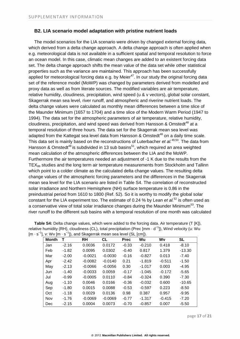
Table S4: Delta change values, which were added to the forcing data. Air temperature (T [K]),

relative humidity (RH), cloudiness (CL), total precipitation (Prec [mm · d−1

]), Wind velocity (u: Wu

[m · s−1

], v: Wv [m · s−1

]), and Skagerrak mean sea level (SL [cm]). Month T RH CL Prec Wu Wv SL Jan -2.16 0.0036 0.0172 -0.33 -0.210 0.418 -8.10

Feb -1.82 0.0095 0.0302 -0.40 0.817 1.379 -13.30

Mar -2.00 -0.0021 -0.0030 -0.16 -0.827 0.013 -7.40

Apr -2.42 -0.0082 -0.0140 0.21 -1.819 -0.511 -1.50

May -2.13 -0.0066 -0.0056 0.30 -1.017 0.003 -4.95

Jun -1.40 -0.0033 0.0059 -0.17 -1.045 -0.172 -5.65

Jul -0.99 -0.0005 0.0110 -0.84 -0.324 0.390 -7.30

Aug -1.10 0.0046 0.0166 -0.36 -0.032 0.600 -10.65

Sep -1.80 0.0015 0.0088 -0.53 -0.597 0.223 -8.50

Oct -1.18 0.0029 0.0136 0.98 0.387 0.957 -9.95

Nov -1.76 -0.0069 -0.0069 -0.77 -1.317 -0.415 -7.20

Dec -2.15 0.0004 0.0073 -0.70 -0.857 0.007 -5.50



page 18 of 21

from Hansson et al.54. The twenty rivers included in the model were assigned to the sub

basins and the relative change in the mass flow between the LIA and MoWP was calculated.

The model river runoff was adapted to the LIA scenario by multiplication of the river data with

the appropriate factor. The resulting delta change factors are listed in Table S5. For the LIA

scenario the riverine and atmospheric nutrient input was adapted by multiplication with

factors (Table S6) derived from Schernewski & Neumann55. Due to a lack of robust data the

atmospheric nutrient loads to the Baltic Sea during the LIA were assumed to be in the order

of 10% of the input during the MoWP55. The experimental LIA scenario model was driven

with these changed forcing data. Similar to the MoWP scenario the model was started with

initial conditions derived from the first LIA scenario version to eliminate the spin off effect.

This LIA scenario was simulated only once because the differences of the ensemble

members of the formerly mentioned MoWP model scenario are very small and do not have Table S5: Delta change factors of riverine freshwater inflow, which were multiplied to the river

runoff data. sub basin river factor Arkona Basin Oder, Peene 1.002099 Belt Sea Schwentine, Trave, Warnow 1.002152 Bornholm Basin Helgeå 1.002125 Bothnian Bay Kemijoki, Lule älv, Ume älv 0.904573 Bothnian Sea Ångerman River, Kokemäenjoki 0.904573 E Gotland Basin Neman, Pregolya, Vistula 1.002118 Gulf of Finland Narva, Neva 1.011357 Gulf of Riga Daugava 1.002122 Kattegat Göta älv 1.002113 NW Gotland Basin Emån-Motala, Mälaren 1.002134

Table S6: Delta change factors of the preindustrial riverine nutrient loads.

river NH4 NO3 PO4 Ångerman River 0.363636 0.545455 1.000000

Daugava 0.078125 0.211640 0.307692

Emån-Motala 0.256410 0.362319 0.500000

Göta älv 0.129870 0.183486 0.500000

Helgeå 0.263158 0.277008 1.000000

Kemijoki 0.088889 0.363636 0.200000

Kokemäenjoki 0.095238 0.253807 0.153846

Lule älv 0.285714 0.972973 1.000000

Mälaren (Norrström) 0.013793 0.120482 0.012384

Narva 0.144928 0.228311 0.222222

Neman 0.093897 0.233463 0.571429

Neva 0.089286 0.444444 0.400000

Oder 0.101754 0.395389 0.101695

Peene 0.101754 0.395389 0.101695

Pregolya 0.093897 0.233463 0.571429

Schwentine 0.101754 0.395389 0.101695

Trave 0.101754 0.395389 0.101695

Ume älv 0.500000 0.857143 1.000000

Vistula 0.063319 0.559543 0.461538

Warnow 0.101754 0.395389 0.101695



page 19 of 21

significance influence on the statistical results. To analyse the consequences of the changed

external forcing on the Baltic Sea model the results from the LIA scenario were statistically

compared with the ones from the reference MoWP scenario.

B3. LIA scenario with modern nutrient loads

The impact of nutrient loads on the oxygen concentration of the Baltic Sea has been

calculated with an additional model experiment. For this experiment the same external

forcing was chosen as for the LIA scenario (cf. Table S4, S5) but nutrient loads were kept at

the same level as in the MoWP scenario.

B4. LIA scenario with wind speed variations

The impact of wind speed on oxygen concentrations in the Eastern Gotland Basin was

studied by two additional LIA scenarios. In the original LIA scenario the delta change

according to Table S4 resulted in a wind speed increased of ~2 % compared to the MoWP

scenario. The additional scenarios were driven (a) by the original wind fields from the MoWP

scenario and (b) by wind fields changed with doubled delta change values compared to the

values presented in Table S4 resulting in an increase of ~4 % compared to the MoWP

scenario.

Figure S11 shows the median oxygen concentration at the central Eastern Gotland station

for the three LIA scenarios. It is obvious, that wind speed changes in the range of the

reconstructions48 do not impact the deep water oxygen concentrations in the LIA scenario.

Furthermore, reconstructions of the North Atlantic Oscillation (NAO) suggest a reduced

NAO for the LIA56 which is related to less strong wind speeds. Decreased wind speed causes

increased age of the deep water57, which is an indicator for less ventilation and low oxygen.

Figure S11: Median oxygen profiles in the central Eastern Gotland Basin for the LIA scenario.

Thick black line: the LIA scenario, thick blue line: LIA scenario with MoWP wind, thick red line: LIA

scenario with doubled delta change in wind fields (cf. Table S4). Shaded area shows the +-1 standard

deviation range.



page 20 of 21

concentrations. These sensitivity studies provide further support to our finding that

temperature decrease is the most important meteorological driver for high oxygen

concentrations during the LIA.

B5. References

40. Neumann, T., Fennel, W. & Kremp, C. Experimental simulations with an ecosystem

model of the Baltic Sea: A nutrient load reduction experiment. Global Biogeochem.

Cy. 16, 7.1–7.19 (2002).

41. Neumann, T. & Schernwski, G. Eutrophication in the Baltic Sea and shifts in nitrogen

fixation analyzed with a3d ecosystem model. J. Mar. Sys. 74, 592–602 (2008).

42. Pacanowski, R. C. & Griffies, S. M. Mom 3.0 manual. Tech. rep., Geophysical Fluid

Dynamics Laboratory (2000).

43. Mutzke, A. Open boundary condition in the gfdl-model with free surface. Ocean

Model. 116, 2–6 (1998).

44. Neumann, T. Climate-change effects on the Baltic Sea ecosystem: A model study. J.

Mar. Sys. 81, 213–224 (2009).

45. Uppala, S. M., Kållberg, P. W., Simmons, A. J., Andrae, U., Da Costa Bechtold, V.,

Fiorino, M., Gibson, J. K., Haseler, J., Hernandez, A., Kelly, G. A., Li, X., Onogi, K.,

Saarinen, S., Sokka, N., Allan, R. P., Andersson, E., Arpe, K., Balmaseda, M. A.,

Beljaars, A. C. M., Van De Berg, L., Bidlot, J., Bormann, N., Caires, S., Chevallier, F.,

Dethof, A., Dragosavac, M., Fisher, M., Fuentes, M., Hagemann, S., Hólm, E.,

Hoskins, B. J., Isaksen, L., Janssen, P. A. E. M., Jenne, R., McNally, A. P., Mahfouf,

J.-F., Morcrette, J.-J., Rayner, N. A., Saunders, R. W., Simon, P., Sterl, A.,

Trenberth, K. E., Untch, A., Vasiljevic, D., Viterbo, P. & Woollen, J. The era-40

reanalysis. Q. J. R. Meteor. Soc. 131, 2961–3012 (2005).

46. Taylor, K. E. PCMDI Report No. 55 - Summarizing multiple aspects of model

performance in a single diagram. Technical report, University of California, Lawrence

Livermore National Laboratory (2000).

47. Meier, M. Baltic Sea climate in the late twenty-first century: a dynamical downscaling

approach using two global models and two emission scenarios. Clim. Dyn. 27, 39–68

(2006).

48. Hansson, D. & Omstedt, A. Modelling the Baltic Sea ocean climate on centennial

time scale: temperature and sea ice. Clim. Dyn., 30, 763–778 (2008).

49. Luterbacher, J. et al. Reconstruction of sea level pressure fields over the Eastern

North Atlantic and Europe back to 1500. Clim. Dyn., 18, 545–561 (2002).

50. Luterbacher, J., Dietrich, D., Xoplaki, E., Grosjean, M. & Wanner, H. European

Seasonal and Annual Temperature Variability, Trends, and Extremes Since 1500.

Science 303, 1499–1503 (2004).

51. Omstedt, A. Modelling the Baltic Sea as thirteen sub-basins with vertical resolution.

Tellus 42, 286–301 (1990).

52. Lean, J., Beer, J. & Bradley, R. Reconstruction of solar irradiance since 1610:

Implications for climate change. Geophys. Res. Let. 22, 3195–3198 (1995).

53. Bard, E., Raisbeck, G., Yiou, F. & Jouzel, J. Solar irradiance during the last 1200

years based on cosmogenic nuclides. Tellus 52, 985–992 (2000).

54. Hansson, D., Eriksson, C., Omstedt, A. & Chen, D. Reconstruction of river runoff to



page 21 of 21

the Baltic Sea, AD 1500–1995. Int. J. Climatol. 31, 696–703 (2011).

55. Schernewski, G. & Neumann, T. The trophic state of the Baltic Sea a century ago: a

model simulation study. J. Mar. Syst. 53, 109–124 (2005).

56. Trouet, V. et al. Persistent Positive North Atlantic Oscillation Mode Dominated the

Medieval Climate Anomaly. Science 324, 78–80 (2009).

57. Meier M. E. H. Modeling the age of Baltic Seawater masses: Quantification and

steady state sensitivity experiments. J.Geophys. Res., 110, C02006,

doi:10.1029/2004JC002607 (2005).


supplementary information - images.nature.com · basins traceable (m. moros unpublished loss on...

Documents