substitution elasticities and investment dynamics … · substitution elasticities and investment...
TRANSCRIPT

WORKING PAPER SERIES
Substitution Elasticities and Investment Dynamics in Two-Country Business Cycle Models
Michael R. Pakko
Working Paper 2002-030B http://research.stlouisfed.org/wp/2002/2002-030.pdf
November 2002 Revised November 2003
FEDERAL RESERVE BANK OF ST. LOUIS Research Division 411 Locust Street
St. Louis, MO 63102
______________________________________________________________________________________
The views expressed are those of the individual authors and do not necessarily reflect official positions of the Federal Reserve Bank of St. Louis, the Federal Reserve System, or the Board of Governors.
Federal Reserve Bank of St. Louis Working Papers are preliminary materials circulated to stimulate discussion and critical comment. References in publications to Federal Reserve Bank of St. Louis Working Papers (other than an acknowledgment that the writer has had access to unpublished material) should be cleared with the author or authors.
Photo courtesy of The Gateway Arch, St. Louis, MO. www.gatewayarch.com

Substitution Elasticities and Investment Dynamics inTwo-Country Business Cycle Models
1. Introduction
Two country applications of equilibrium business cycle methodology — international
real business cycle (IRBC) models — have been successful in matching many features of
cyclical fluctuations and comovements across countries. One-commodity, two-county models
[e.g. Cantor and Mark (1988), Baxter and Crucini (1993), Backus, Kehoe and Kydland (1992),
do reasonably well in matching within-country patterns of volatility, persistence and
comovement among macroeconomic variables. Two-good extensions of the baseline model,
as in Backus, Kehoe and Kydland (1994, 1995) [hereafter, BKK] have extended these results
to replicating some of the patterns of trade flows and terms-of-trade fluctuations. For
example, the baseline two-good model in BKK (1995) predicts persistence of terms-of-trade
fluctuations, the correlation between the terms of trade and net exports, and the
countercyclicality of net exports that are generally consistent with the data. BKK (1994) also
show that the lagged cross-correlation function between the terms of trade and net exports
displays a “J-curve” relationship that is similar to that seen in the data.
Table 1 summarizes some of the empirical regularities that have been the focus of
the IRBC literature. For example, domestic output, consumption and investment are
positively correlated, and show a consistent pattern of relative variability. Fluctuations in
net exports are consistently countercyclical and generally negatively correlated with the
terms of trade. IRBC models have been successful at matching these general features of
the data.

1Pakko (1998) suggests that comparing the correlations of consumption with domesticoutput to correlations of consumption with world output (as in Lewis, 1996) provides a morerobust characterization of the quantity puzzle. The conventional characterization will beconsidered in this paper, however.
Table 1 also shows properties of international business cycles which have been
more difficult to generate in typical IRBC models. BKK (1995) refer to two of these
anomalies as the “quantity puzzle” and the “price puzzle”. First, models tend to predict
very high cross-country consumption correlations, whereas the data in Table 1 show that
consumption correlations tend to be lower than output correlations.1 The price puzzle
refers to the variability of the terms of trade. Models tend to predict a standard deviation
for the terms of trade that is much lower than in the data.
An additional discrepancy—the “international comovement puzzle” (Baxter,
1995)—refers to the cross-country correlations of factor inputs. In the data, investment and
employment are positively correlated across countries, whereas models tend to imply
negative correlations. The data in Table 1 show that for each of the countries considered,
domestic investment is positively correlated with investment in the rest of the OECD.
Table 2A illustrates the robustness of this empirical regularity, showing bilateral cross
country investment correlations. Only two of the bilateral correlations in Table 2A have a
negative sign, and in each case the magnitude is insignificantly different from zero. Table
2B shows that the corresponding bilateral correlations for employment also display a
marked tendency toward positive comovement. However, IRBC models driven by shocks
to relative productivity tend to predict negative correlations for these variables.
In this paper, I address the international comovement puzzle of cross-country
investment correlations directly by introducing investment adjustment costs, and in so
doing, identify an additional anomaly that is related to a basic dynamic property of typical
models: The model dynamics that generate countercyclical net exports and negative co-
movement between net exports and the terms of trade – as seen in the data – are also
related to the counterfactual prediction of negative cross-country investment and
employment correlations. When investment adjustment costs are introduced to reverse the
cross-country investment correlation, the implications for net exports and the terms of trade
cyclicality are reversed, and the J-curve pattern is no longer a feature of the simulated
dynamics. In this sense, the ability of standard models to replicate key empirical
regularities is shown to be fragile for typical calibrations.
An important parameter for generating more robust implications of the model is
the elasticity of substitution between foreign and domestic goods. If the two types of goods
are compliments instead of being substitutes, productivity shocks are associated with
demands for domestic goods and imports being tied more tightly to relative shares. This
magnifies the positive response of import demand when consumption rises following a
positive productivity shock, enhancing the tendency of the model to predict countercyclical
trade balance dynamics. Assuming a low substitution elasticity, the model with investment
adjustment costs is shown to be capable of generating positive cross-country correlations
of investment and work effort, as well as countercyclical net exports and a negative
correlation between net exports and the terms of trade— retaining the J-curve pattern. This
specification moves the model closer toward more realistic implications with regard to the
quantity and price puzzles as well.
The outline of the paper’s exposition is as follows: Section 2 describes a baseline
model and shows how the introduction of investment adjustment costs affects cross-country
investment correlations and the dynamics of the terms of trade and net exports. Section 3
explores the sensitivity of these results to the elasticity of substitution between foreign and

Et ��
t�0βtU(Ct,1�Nt)
Xt � AtF(Kt,Nt) � AtKαt N 1�α
t ,
Yt � A �
t F(K �
t ,N �
t ) � A �
t K �αt N �1�α
t .
H(xt, yt) � Ct � It (1)
H �(x �
t , y �
t ) � C �
t � I �
t (1*)
domestic goods, showing that an assumption of complementarity provides a more robust fit
between the model and the data. Section 4 presents some basic empirical estimates of the
relevant elasticity parameter to support the relevance of this finding. Section 5 concludes.
2. Baseline Economy
2.1 Preferences and Technology
The baseline model economy is that used by BKK (1994, 1995). It consists of two
countries, each of which is inhabited by an infinitely-lived representative agent. Both
agents have expected utility functions of the form
where Ct and Nt are consumption and work effort, and U(Ct,1-Nt)=[Ctθ (1-Nt)1-θ]1-γ/(1-γ).
Production takes place in each country using capital and labor. The home country
produces Xt of the x-good while the foreign country produces Yt of the y-good:
Consumption and investment are composites of domestic goods and imports,
where H(x,y) and H*(x*,y*) are Armington aggregator functions of the CES form:
H(xt, yt) � [ax 1�ηt � (1�a)y 1�η
t ]1
1�η H �(x �
t , y �
t ) � [(1�a)x �1�ηt � ay �1�η
t ]1
1�η

2Papers departuring from the assumption of complete asset markets include Baxterand Crucini (1995), Arvanitis and Mikkola (1996), Kollman (1996), Heathcote and Perri(2002), and Kehoe and Perri (2002).
Kt�1 � (1�δ)Kt � It (2)
K �
t�1 � (1�δ)K �
t � I �
t (2*)
Pt � [�H(xt,yt)/�yt]/[�H(xt,yt)/�xt] ,
NXt � xt� � Pt yt .
AA
AA
t
t
xx
yx
xy
yy
t
t
t
t
�
�
�
�
�
��
�
�� �
�
��
�
���
�
��
�
�� �
�
��
�
��
1
1
1
1* * * .
The elasticity of substitution between domestic goods and imports is 1/η. The parameter a
determines the relative shares of domestic goods and imports in consumption and
investment.
Capital stocks in the two countries evolve according to
where δ is the depreciation rate of capital.
The equilibrium relative price of the home country’s import (the terms of trade) can
be computed from the marginal rate of substitution implicit in the Armington aggregator:
and the trade balance for the home country can be expressed in units of the domestic good as
The exogenous technology shock variables A and A* follow a joint AR(1) process,
International asset markets are assumed to be complete in the sense that agents have
access to a complete array of state-contingent assets, so the equilibrium will be Pareto
optimal and can be found as the solution to a social-planner’s problem.2 With two equal-
sized countries, the social planner’s objective can be represented as maximizing the simple

3E.g. King, Plosser and Rebelo (1988).
AtF(Kt,Nt) � xt � x �
t (3)
A �
t F(K �
t ,N �
t ) � yt � y �
t (3*)
sum of the two agents’ discounted expected utility, subject to constraints (1), (1*), (2), (2*)
and the resource constraints:
2.2 Model Dynamics
Dynamic simulations of the model are calculated as the solution to a log-linear
approximation of the nonlinear system of optimality conditions and constraints, using
standard methods.3 For all the second-moment results reported in this paper, the HP filter
is applied using a frequency-domain representation of the HP filter’s variance transfer
function to the model’s implied population moments [as in King and Rebelo (1993)].
The model is calibrated using the baseline parameter values given in Table 3, with
most parameter values following those used in BKK (1995). Assuming quarterly time
periods, the discount factor is consistent with a 4% real interest rate and an annual capital
depreciation rate of 10%. The Cobb-Douglas parameters in utility and production are set
so that the fraction of time spent working is 0.3 and that labor’s share of output is 0.64.
The parameters of the Armington aggregator are chosen to imply an import share of 0.15
and a baseline value for the elasticity of substitution between domestic goods and imports
of 1.5. The parameters governing technology process are those estimated by BKK (1992):
ρxx=ρyy=0.906, ρxy=ρyx=0.088, and var(ε)=var(ε*)=.08325.
The row labeled “baseline” in Table 4 reports some of the key implications of this
specification of the model. Consumption and investment are both highly correlated with

4Table 1 shows that the U.S. is the exception to the general regularity that net exportsand the terms of trade are negatively correlated.
output, the cross-country output correlation is positive, and net exports are negatively
correlated with both output and the terms of trade.4
The IRBC “puzzles” are also clear: Cross-country consumption correlations are
higher than corresponding output correlations, the standard deviation of the terms of trade
is far lower than seen in the data, and the model implies negative correlations of investment
and employment across countries.
The interrelatedness of these features of the model is illustrated in Figure 1, which
shows impulse-response functions for a positive technology shock to the home country’s
production function. The increase in the home country’s marginal product of capital attracts
investment, absorbing resources from abroad (hence, inducing countercyclical net exports).
However, this fundamental feature of the dynamics also is responsible for the negative cross-
country investment correlation. The terms of trade respond to changes in the relative supply
of home- and foreign-produced goods, which is magnified by the response of work-effort to
the change in the relative marginal product of labor across countries. Given the assumption
of complete asset markets, consumption would co-move perfectly if not for the substitution
of leisure for consumption implied by the patterns of work-effort in response to marginal
products of labor. However, this feature also generates the counterfactual implication of
negative co-movement of employment across countries.
The initial responses of investment and work-effort to productivity shocks dominate
the dynamics summarized by the cross-country correlations shown in Table 4. Nevertheless,
the impulse-response functions in Figure 1 show that the longer-run dynamics of these
variables are characterized by positive comovement. As the direct effects of the productivity

Kt�1 � (1�δ)Kt � φ(It/Kt)Kt (2a)
K �
t�1 � (1�δ)K �
t � φ(I �
t /K �
t )K �
t (2a*)
shock dissipate, accumulated capital is optimally shared more equally across countries
giving rise to a longer-run component of dynamics associated with a positive cross-country
investment correlation. Moreover, the effect of these capital-stock dynamics on the marginal
product of labor also imply a longer-run positive comovement of work-effort across
countries. The introduction of a friction to dampen the initial impact-responses of
investment and work effort to relative productivity shocks should therefore work toward
generating positive (or at least, less negative) cross-country correlations of these variables.
One direct approach to dampening the initial response of investment is the introduction of
investment adjustment costs.
2.3 Investment Adjustment Costs
Investment adjustment costs are modeled as a friction that reduces the
effectiveness of investment in proportion to deviations from the steady-state path. In
particular I employ the specification for investment adjustment costs used by Baxter and
Crucini (1993, 1995), modifying the capital accumulation equations to:
where the adjustment cost function has the properties φ(·)>0, φ�(·)>0, φ�(·)<0. The
function φ(·) is calibrated so that the steady state investment/capital ratio is the same as in
the model without adjustment costs and the steady-state value of Tobin’s q is 1, leaving
one free parameter, which can be described as the elasticity of the investment/capital ratio
with respect to Tobin’s q, ζ=[φ�(·)/φ�(·)](I/K). The results reported below use an elasticity

value of ζ=-4, which is sufficient to generate positive cross-country investment correlations
with all other parameters unchanged from the baseline case.
The second row of figures in Table 4 report the implied moments of the model with
investment adjustment costs. Note that this added friction has the intended result: The
volatility of investment is lower and the cross-country correlation of investment spending
is now positive. The addition of investment adjustment costs also raises the variability of
the terms of trade and lowers that of output. Moreover, cross country-consumption
correlations are lower and cross-country output correlations are higher in the adjustment-
cost economy. These modifications work in the direction of resolving both the quantity
puzzle and the price puzzle. However, net exports are now significantly procyclical, and
the terms of trade covaries positively with net exports. A small dampening of the
investment-flow channel of the model results in a complete reversal of the cyclical
behavior of these two variables.
Figures 2 and 3 illustrates how the introduction of investment adjustment costs
alters the dynamic response of the model. A positive productivity shock in the home
country gives rise to a much smaller increase in investment (as expected). Net exports now
rise, rather than fall as an immediate consequence of the shock. Moreover, note that the J-
curve pattern observed in the impulse-response function for the terms of trade in the
baseline case is no longer a feature of the simulation with investment adjustment costs.
3. The Role of the Substitution Elasticity
An important parameter governing the model’s implied dynamics is the elasticity of
substitution between foreign and domestic goods. The sensitivity of model dynamics to
changes in the substitution elasticity has been noted in the literature. For example, the role

of this elasticity parameter in endowment economies has been considered by Hagiwara
(1994) [terms of trade fluctuations] and Pakko (1997) [the quantity puzzle]. BKK (1995)
conduct a sensitivity analysis of the substitution elasticity in regard to both the quantity and
price puzzles, and Heathcote and Perri (2002) found it to be an important parameter in their
investigation of international comovements in environments with limited asset-trade.
Lowering the elasticity of substitution has the effect of increasing the volatility of
the terms of trade—directly addressing the price puzzle. And because lower
substitutability between domestic goods and imports reduces incentives to substitute
production locations, cross-country correlations of output are higher, as are cross-country
correlations of investment and labor—addressing both the quantity puzzle and the
international comovement puzzle.
The rows of Table 4 labeled “unit elasticity” and “low elasticity” correspond to
simulations of the model for values of 1/η=1 and 2/3, respectively. The baseline versions
of these case is similar are many respects to the high-elasticity version already considered.
The performance of the model is improved marginally along the lines found by BKK, but
their puzzles remain. Other implied second moments are roughly the same.
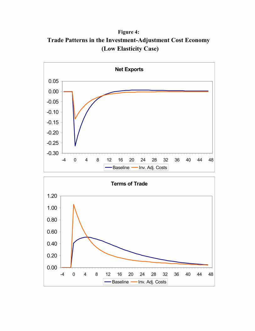
After introducing investment adjustment costs, there are some striking differences
between the high-elasticity and lower-elasticity economies. It is still true that adjustment
costs lower the volatility of investment and can reverse the negative cross-country
correlation between investment levels. In the lower elasticity cases, however, net exports
remain countercyclical and continue to covary negatively with the terms of trade. Figure 4
illustrates the trade dynamics in response to a home-country productivity shock for the low
elasticity case. The non-monotonic path for net exports is retained in this case, even after

5For example, with an elasticity as low as 0.025, the model with investmentadjustment costs generates a cross-country consumption correlation of 0.48 and a cross-country output correlation of 0.50.
the introduction of investment adjustment costs. Hence, the model continues to generate
the J-curve relationship between net exports and the terms of trade.
Note also that the introduction of investment adjustment costs tends to reinforce
the low-elasticity version’s ability to remedy the BKK quantity and price puzzles.
Consumption correlations are higher while output correlations lower; term of trade
variability is higher while output variability is lower. BKK (1995) show that lowering the
elasticity of substitution can only go so far in resolving the quantity puzzle in the baseline
model. In the model with investment adjustment costs, however, very low elasticity
parameterizations are associated with consumption correlations that are lower than output
correlations.5
4. Realistic Values for the Elasticity of Substitution
The low-elasticity version of the model with investment adjustment costs performs
well with respect to a number of issues, but how realistic is that parameterization? There
exists a large body of literature measuring import demand and export supply elasticities
[e.g. Stern et al., (1976); Whalley (1985)]. This work suggests elasticities in the range of
one to two, providing the baseline estimate used in standard models.
However, these measures are not conceptually identical to the substitution elasticity
parameterized in the model. Empirical elasticity studies have tended to be conducted on a
highly disaggregated basis, whereas the relevant empirical counterparts to the commodities
represented in the model are bundles of goods. Some goods may be very close substitutes,

6In a model with nontraded goods modeled explicitly, Tesar (1993) Stockman andTesar (1995) found that the elasticity of substitution between traded and nontraded goods wasa crucial parameter, with low values generating more realistic simulation results.
other highly differentiated, some nontraded, some subject to trade distortions, etc. The
relevant elasticity to consider is not a pure preference or technological parameter, but a
composite that reflects a mixture of factors.6 The appropriate elasticity might be
considerably lower than the measured substitutability of specific categories of traded
goods.
Table 5 presents some simple regression estimates of the substitution elasticity
using aggregate OECD data. Two measures of empirical counterparts to the ratio y/x ratio
(along with the associated relative prices) are used: The first is simply the ratio of imports
to exports, the second is the ratio of imports to output minus net exports, as literally
implied by the Armington aggregator specification in the model. The estimates are found
using ordinary least-squares regression of the quantity ratio on the price ratio, in which the
variables are logged and first-differenced. An AR(1) term is included to adjust for serially
correlated error terms.
The elasticity estimates suggest that the low-elasticity calibration of the model is a
reasonable specification. Using the import/export ratio as the relevant measure, point
estimates of the substitution elasticity are uniformly less than one. Using the alternative
measure of relative quantities and prices, estimates of substitution elasticities are even lower.
In fact, the estimated elasticity for this specification yields estimates that are not significantly
different from zero for most of the countries in the sample.

5. Discussion and Conclusions
This paper has demonstrated the importance of inter-country capital flows for the
dynamics of a standard two country real business cycle model, and the resulting sensitivity
of the models predictions to the introduction of a friction to cross-country investment flows.
The addition of investment adjustment costs to the model reverses the implied cyclical
behavior of net exports and the terms of trade for a baseline parameterization. However, the
model with investment adjustment costs is capable of generating countercyclical net exports
and negative comovement between net exports and the terms of trade for calibrations that
assume a low elasticity of substitution between foreign and domestic goods.
The introduction of investment adjustment costs is a very simple and straightforward
approach to resolving the model’s implications for cross-country investment correlations.
Other approaches to resolving the IRBC puzzles similarly address the margin of
substitutability, particularly with respect to investment. Baxter and Farr (2001) consider the
role of variable factor utilization, allowing for substitutability along intensive margins to
dampen substitution along extensive margins. Maffezzoli (2000) models human capital as
an additional factor of production that tends to dampen cross-country fluctuations in capital
accumulation. Heathcote and Perri (2002) examine a model of “portfolio autarky” that
relaxes the connection between the marginal products of capital in the home and foreign
countries, lowering cross-country investment correlations.
Investment adjustment costs have been introduced in this paper not necessarily as
an alternative solution to the puzzles of the IRBC literature, but to illustrate a more general
feature of a wide class of models than can help resolve those puzzles. That is, the
assumption of complementarity between domestic goods and imports provides a more

robust specification of the model which can better match the data in the adjustment-costs
model, and is likely to help in other settings as well. Indeed, Heathcote and Perri (2002)
found that their model of “portfolio autarky” matched the data best for values between 0.5
and 1.0, and used an estimated value of 0.9.
The model simulations and aggregate elasticity estimates presented in this paper
suggest that complementary between domestic goods and imports in this range are realistic,
and provide for a more parsimonious fit between model dynamics and the data.

References
Arvanitis, Athanasios V. and Anne Mikkola, “Asset-Market Structure and International TradeDynamics,” AEA Papers and Proceedings (1996), 67-70.
Backus, David, Patrick Kehoe, and Finn Kydland, "Dynamics of the Trade Balance and theTerms of Trade: The J-Curve?", American Economic Review 84 (1994): 84-103.
__________, "International Real Business Cycles," Journal of Political Economy 100 (1992):745-75.
__________, "International Business Cycles: Theory and Evidence," in, Thomas F. Cooley,ed., Frontiers of Business Cycle Research, (Princeton: Princeton University Press,1995).
Backus, David K. and Gregor W. Smith. “Consumption and Real Exchange Rates in Dynamic Economies with Non-Traded Goods.” Journal of International Economics 35(November 1993), 297-316.
Baxter, Marianne, “International Trade and Business Cycles,” in G. Grossman and K. Rogoff,Eds., Handbook of International Economics III, Amsterdam: North-Holland, pp. 1801-64.
__________ and Dorsey D. Farr, “Variable Factor Utilization and International Business Cycles,”NBER Working Paper 8392 (July 2001).
__________ and Mario J. Crucini, "Business Cycles and the Asset Structure of Foreign Trade",International Economic Review 36 (1995): 821-854.
__________ "Explaining Saving-Investment Correlations," The American Economic Review 83(1993): 416-436.
Cantor, Richard and Nelson C. Mark, "The International Transmission of Real Business Cycles," International Economic Review 29 (1988): 493-507.
Devereux, Michael B., Allan W. Gregory, and Gregor W. Smith, "Realistic Cross-CountryConsumption Correlations in a Two-Country, Equilibrium, Business Cycle Model,"Journal of International Money and Finance 11 (1992): 3-16.
Hagiwara, May, "Volatility in the Terms of Trade with Non-Identical Preferences," Journal ofInternational Money and Finance 13 (1994): 319-341.
Heathcote, Jonathan and Fabrizio Perri, “Financial Autarky and International Business Cycles,”Journal of Monetary Economics 49:3 (2002), 601-627.
Kehoe, Patrick J. and Fabrizio Perri, “International business Cycles With EndogenousIncomplete Markets,” Econometrica 70:3 (2002), 907-928.

King, Robert G., and Sergio T. Rebelo, “Low Frequency Filtering and Real Business Cycles,”Journal of Economic Dynamics and Control 20 (1993), 207-31.
Kollmann, Robert, "Incomplete Asset Markets and the Cross-Country Consumption CorrelationPuzzle," Journal of Economic Dynamics and Control 20 (1996), 945-961.
Lewis, Karen K., “What can Explain the Apparent Lack of International Consumption RiskSharing? Journal of Political Economy 104 (1996), 218-240.
Lucas, Robert E, Jr. “Interest Rates and Currency Prices in a Two-Country World.” Journal ofMonetary Economics 10 (November 1982), 335-359.
Maffezzoli, Marco. “Human Capital and International Real Business Cycles,” Review ofEconomic Dynamics 3 (2000), 137-65.
Obstfeld, Maurice. “Are Industrial-Country Consumption Risks Globally Diversified?” inLeonardo Leiderman and Assaf Razin, eds., Capital Mobility: The Impact on Consumption, Investment and Growth, (Cambridge University Press, 1994), 13-44.
Pakko, Michael R. "Characterizing Cross-Country Consumption Correlations," Review ofEconomics and Statistics 80 (1998), 169-174.
__________, "Low Cross-Country Consumption Correlations and International Risk Sharing: AreThey Really Inconsistent?” Review of International Economics 5 (1997), 386-400.
Stern, Robert, Jonathan Francis, and Bruce Shumacher, Price Elasticities in International Trade:An Annotated Bibliography, London: Macmillan, 1976.
Stockman, Alan C., and Harris Dellas, "International Portfolio Non-diversification andExchange Rate Variability," Journal of International Economics 26 (1989): 271-89.
Stockman, Alan C., and Linda Tesar, "Tastes and Technology in a Two-Country Model of theBusiness Cycle: Explaining International Comovements," The American EconomicReview 85 (1995): 168-85.
Tesar, Linda L., "International Risk-Sharing and Non-Traded Goods," Journal of InternationalEconomics 35 (1993): 69-89.
Wen, Yi, “Demand-Driven Business Cycles: Explaining Domestic and InternationalCovovements,” Unpublished Manuscript, Cornell University (April 17, 2001).
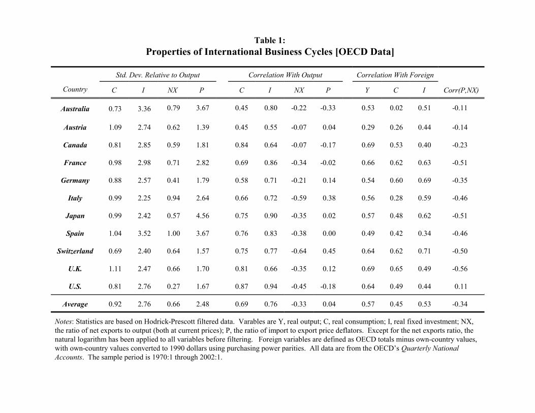
Table 1: Properties of International Business Cycles [OECD Data]
Std. Dev. Relative to Output Correlation With Output Correlation With Foreign
Country C I NX P C I NX P Y C I Corr(P,NX)
Australia 0.73 3.36 0.79 3.67 0.45 0.80 -0.22 -0.33 0.53 0.02 0.51 -0.11
Austria 1.09 2.74 0.62 1.39 0.45 0.55 -0.07 0.04 0.29 0.26 0.44 -0.14
Canada 0.81 2.85 0.59 1.81 0.84 0.64 -0.07 -0.17 0.69 0.53 0.40 -0.23
France 0.98 2.98 0.71 2.82 0.69 0.86 -0.34 -0.02 0.66 0.62 0.63 -0.51
Germany 0.88 2.57 0.41 1.79 0.58 0.71 -0.21 0.14 0.54 0.60 0.69 -0.35
Italy 0.99 2.25 0.94 2.64 0.66 0.72 -0.59 0.38 0.56 0.28 0.59 -0.46
Japan 0.99 2.42 0.57 4.56 0.75 0.90 -0.35 0.02 0.57 0.48 0.62 -0.51
Spain 1.04 3.52 1.00 3.67 0.76 0.83 -0.38 0.00 0.49 0.42 0.34 -0.46
Switzerland 0.69 2.40 0.64 1.57 0.75 0.77 -0.64 0.45 0.64 0.62 0.71 -0.50
U.K. 1.11 2.47 0.66 1.70 0.81 0.66 -0.35 0.12 0.69 0.65 0.49 -0.56
U.S. 0.81 2.76 0.27 1.67 0.87 0.94 -0.45 -0.18 0.64 0.49 0.44 0.11
Average 0.92 2.76 0.66 2.48 0.69 0.76 -0.33 0.04 0.57 0.45 0.53 -0.34
Notes: Statistics are based on Hodrick-Prescott filtered data. Varables are Y, real output; C, real consumption; I, real fixed investment; NX,the ratio of net exports to output (both at current prices); P, the ratio of import to export price deflators. Except for the net exports ratio, thenatural logarithm has been applied to all variables before filtering. Foreign variables are defined as OECD totals minus own-country values,with own-country values converted to 1990 dollars using purchasing power parities. All data are from the OECD’s Quarterly NationalAccounts. The sample period is 1970:1 through 2002:1.

Table 2A: Cross-Country Investment Correlations
Australia Austria Canada France Germany Italy Japan Spain Sweden U.K. U.S.
Australia 1.00
Austria 0.12 1.00
Canada 0.60 0.19 1.00
France 0.38 0.26 0.42 1.00
Germany 0.15 0.51 0.14 0.54 1.00
Italy 0.18 0.29 0.36 0.72 0.45 1.00
Japan 0.23 0.30 0.27 0.61 0.56 0.57 1.00
Spain 0.15 0.03 0.33 0.69 0.11 0.61 0.41 1.00
Sweden 0.46 0.38 0.43 0.77 0.55 0.60 0.56 0.44 1.00
U.K. 0.32 -0.08 0.18 0.32 0.21 0.22 0.29 0.26 0.32 1.00
U.S. 0.43 0.38 0.16 0.23 0.51 0.22 0.39 -0.01 0.48 0.44 1.00
Averages 0.30 0.24 0.31 0.49 0.37 0.42 0.42 0.30 0.50 0.25 0.32
Notes: See Notes to Table 2.
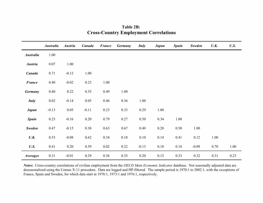
Table 2B: Cross-Country Employment Correlations
Australia Austria Canada France Germany Italy Japan Spain Sweden U.K. U.S.
Australia 1.00
Austria 0.07 1.00
Canada 0.71 -0.12 1.00
France 0.40 -0.02 0.23 1.00
Germany 0.40 0.22 0.35 0.49 1.00
Italy 0.02 -0.14 0.05 0.46 0.36 1.00
Japan -0.13 0.05 -0.11 0.23 0.33 0.29 1.00
Spain 0.23 -0.16 0.20 0.79 0.27 0.50 0.34 1.00
Sweden 0.47 -0.15 0.38 0.63 0.67 0.49 0.20 0.50 1.00
U.K. 0.53 -0.08 0.62 0.34 0.18 0.10 0.14 0.41 0.12 1.00
U.S. 0.41 0.20 0.59 0.02 0.22 -0.13 0.18 0.18 -0.09 0.70 1.00
Averages 0.31 -0.01 0.29 0.36 0.35 0.20 0.15 0.33 0.32 0.31 0.23
Notes: Cross-country correlations of civilian employment from the OECD Main Economic Indicator database. Not seasonally adjusted data aredeseasonalized using the Census X-11 procedure. Data are logged and HP-filtered. The sample period is 1970:1 to 2002:1, with the exceptions ofFrance, Spain and Sweden, for which data start in 1978:1, 1973:1 and 1976:1, respectively.

Table 3:Benchmark Parameter Values
Description Symbol Value
Preferences Discount factor � 0.99
Intertemporal substitution � 2.0
Consumption share � 0.34
Technology Capital’s share � 0.36
Depreciation rate of capital � 0.025
Trade Substitution Elasticity 1/η 1.50
Import Share sy = sx* 0.15
Forcing Processes AR Coefficient Matrix A0 906 0 0880 088 0 906. .. .
�
��
�
��
Cross-Correlation of Shocks �XY 0.258
Shock Variance �ε2 0.08325

Table 4:International Business Cycle Properties of Theoretical Economies
Std, Dev. Relative to Output Correlation With Output Correlation With Foreign
C I NX P C I NX P Y C I N Corr(P,NX)
Data* 0.92 2.76 0.66 2.48 0.69 0.76 -0.33 0.04 0.57 0.45 0.53 0.26† -0.34
Normal Elasticity (3/2)
Baseline 0.48 3.28 0.30 0.34 0.90 0.93 -0.61 0.49 0.10 0.81 -0.53 -0.49 -0.37
Inv. Adj. Costs 0.67 1.62 0.07 0.81 0.96 0.99 0.61 0.63 0.22 0.72 0.19 -0.41 0.99
Unit Elasticity
Baseline 0.49 3.24 0.31 0.42 0.91 0.93 -0.63 0.51 0.13 0.78 -0.51 -0.42 -0.59
Inv. Adj. Costs 0.69 1.72 0.06 0.98 0.97 0.99 -0.59 0.60 0.27 0.67 0.11 -0.04 -0.97
Low Elasticity (2/3)
Baseline 0.50 3.22 0.34 0.50 0.92 0.93 -0.64 0.52 0.16 0.75 -0.48 -0.35 -0.72
Inv. Adj. Costs 0.72 1.81 0.17 1.14 0.99 0.99 -0.58 0.58 0.33 0.62 0.04 0.48 -0.99
* The “Data” row refers to averages of the statistics reported in Table 1. † Average of bilateral correlations reported in Table 2B.

Table 5:Estimates of Substitution Elasticities*
Relative Quantity Definition:
Country IM/EX IM/(Y-EX)
Australia -0.68(0.194)
-0.27(0.093)
Austria -0.63(0.141)
-0.35(0.122)
Canada -0.77(0.157)
-0.00(0.145)
France -0.34(0.095)
-0.08(0.060)
Germany -0.82(0.123)
-0.11(0.089)
Italy -0.50(0.139)
-0.04(0.099)
Japan -0.38(0.095)
-0.02(0.061)
Spain -0.64(0.142)
-0.33(0.073)
Switzerland -0.55(0.101)
-0.10(0.090)
U.K -0.35(0.145)
0.09(0.082)
U.S. -0.49(0.172)
-0.14(0.109)
(Standard errors in parentheses.)
*Regressions of quantity ratios on relative prices (loggedfirst-differences), usingOLS with first-order autocorrelationadjustment.

Output
-0.40
0.00
0.40
0.80
1.20
1.60
-4 0 4 8 12 16 20 24 28 32 36 40 44 48Home Foreign
Investment
-3.00
-2.00
-1.00
0.00
1.00
2.00
3.00
4.00
5.00
-4 0 4 8 12 16 20 24 28 32 36 40 44 48Home Foreign
Consumption
0.00
0.40
0.80
-4 0 4 8 12 16 20 24 28 32 36 40 44 48Home Foreign
Work Effort
-0.30
0.00
0.30
0.60
-4 0 4 8 12 16 20 24 28 32 36 40 44 48Home Foreign
Home Net Exports
-0.25
-0.20
-0.15
-0.10
-0.05
0.00
0.05
0.10
-4 0 4 8 12 16 20 24 28 32 36 40 44 48
Home Terms of Trade
0.00
0.05
0.10
0.15
0.20
0.25
0.30
0.35
0.40
-4 0 4 8 12 16 20 24 28 32 36 40 44 48
Figure 1:Responses to a Positive Productivity Shock in the Home Country

Home and Foreign Investment
-2.00
-1.00
0.00
1.00
2.00
3.00
4.00
5.00
-4 0 4 8 12 16 20 24 28 32 36 40 44 48
Home Baseline Home w/Inv. Adj. CostsForeign Baseline Foreign w/Inv. Adj. Costs
Figure 2:Investment Dynamics with Adjustment Costs

Net Exports
-0.25
-0.20
-0.15
-0.10
-0.05
0.00
0.05
0.10
-4 0 4 8 12 16 20 24 28 32 36 40 44 48Baseline Inv. Adj. Costs
Terms of Trade
0.000.100.200.300.400.500.600.700.800.90
-4 0 4 8 12 16 20 24 28 32 36 40 44 48
Baseline Inv. Adj. Costs
Figure 3:Trade Patterns in the Investment-Adjustment Cost Economy
Net Exports
-0.30
-0.25
-0.20
-0.15
-0.10
-0.05
0.00
0.05
-4 0 4 8 12 16 20 24 28 32 36 40 44 48Baseline Inv. Adj. Costs
Terms of Trade
0.00
0.20
0.40
0.60
0.80
1.00
1.20
-4 0 4 8 12 16 20 24 28 32 36 40 44 48Baseline Inv. Adj. Costs
Figure 4:Trade Patterns in the Investment-Adjustment Cost Economy
(Low Elasticity Case)