dual elasticities of substitution - economicseconomics.ucr.edu/papers/papers01/01-26.pdf · dual...
TRANSCRIPT

April 2004
Dual Elasticities of Substitution
by
Kusum MundraSan Diego State University
and
R. Robert RussellUniversity of California, Riverside1
Abstract
We argue that, for more than two inputs, different elasticity of substitution con-
cepts must be used to answer different questions about substitutability among in-
puts. To assess the effects of price changes, direct elasticities should be used; to as-
sess the effects of quantity changes, dual elasticities should be used. (Direct) Allen-
Uzawa elasticities are ubiquitous; (direct) Morishima elasticities are gradually
working their way into the literature. Dual Allen-Uzawa and Morishima elastici-
ties (for multiple-output, non-homogeneous technologies) have been formulated but
have not yet been applied. We show that the dual Allen-Uzawa elasticity is identical
to the Hicks elasticity of complementarity (for a single output) iff there are con-
stant returns to scale, an assumption we easily reject when we apply each of these
these elasticity concepts to the Swiss labor market for domestic and guest workers.
J.E.L. classification numbers: D2 and J0.
1 Email addresses: [email protected] and [email protected]. We are grateful to ChrisNichol for useful comments and to Aman Ullah for valuable advice. We have also benefited fromthe discussion of our paper in the UCR Theory Colloquium.

1. Introductory Remarks.
The elasticity of substitution was introduced by Hicks [1932] as a tool for analyzing capital
and labor income shares in a growing economy with a constant-returns-to-scale technology
and neutral technological change. Defined as the logarithmic derivative of the capital/labor
ratio with respect to the technical rate of substitution of labor for capital, the elasticity is
higher the “easier” is the substitution of one input for the other (the lesser is the degree
of “curvature” of the isoquant). Under the assumption of cost-minimizing, price-taking
behavior, it is the logarithmic derivative of the capital/labor ratio with respect to the factor-
price ratio (the ratio of the wage rate to the rental rate on capital), and it yields immediate
(differential) qualitative and quantitative comparative-static information about the effect on
relative income shares of changes in factor price ratios.
Under the Hicks predicates, the inverse of the elasticity—the logarithmic derivative of
the technical rate of substitution of labor for capital (the factor shadow-price ratio) with
respect to the capital/labor ratio—contains the same information, but larger values indi-
cate “less easy” substitution of the two factors for one another (greater “curvature” of
the isoquant). Under the assumption of competitive factor markets, it yields immediate
comparative-static information about the effect on (absolute and relative) income shares of
changes in factor quantity ratios.
Thus, whether one is interested in the effects of changes in factor-price ratios on factor-
quantity ratios or the effects of changes in quantity ratios on price ratios (and in each
case the effects on relative factor shares), the Hicksian two-factor elasticity of substitution
provides complete (differential) qualitative and quantitative comparative-static information.
But matters get more complicated when one’s analysis of substitutability and the compara-
tive statics of relative income shares entails more than two factors of production. Prominent
examples in the literature include the analyses of
1

• the effect of energy-cost explosions using KLEM (capital, labor, energy, materials) data
(e.g., Berndt and Wood [1975], Davis and Gauger [1996], and Thompson and Taylor
[1995]),
• the effect of increases in human capital (or in educational attainment) on the relative
wages of skilled and unskilled labor, with capital as a third important input (e.g.,
Griliches [1969], Johnson [1970], Kugler, Muller, and Sheldon [1989], and Welch [1970]),
• the substitutability of (multiple) monetary assets (e.g., Barnett, Fisher, and Serletis
[1992], Davis and Gauger [1996], and Ewis and Fischer [1985]),
• the effect of increases in the number of guest workers on resident and non-resident labor,
with capital and other inputs as well (e.g., Kohli [1999]),
and
• the effect of immigration on the relative wages of domestic and immigrant labor (e.g.,
Grossman [1982], Borjas [1994], and Borjas, Freeman, and Katz [1992, 1996]).
The first issue that arises is that there exist more than one generalization of the Hicksian
two-variable elasticity of substitution. Allen and Hicks [1934] and Allen [1938] suggested two
generalizations. One, further analyzed by McFadden [1963], eventually lost favor because it
does not allow for optimal adjustment of all inputs to changes in factor prices. The other,
further analyzed by Uzawa [1962], became the dominant concept; perhaps tens of thousands
of “Allen-Uzawa elasticities” have been estimated. Later, Morishima [1967] and Blackorby
and Russell [1975, 1981, 1989] proposed an alternative to the Allen-Uzawa elasticity; the
latter argued that this “Morishima elasticity” has attractive properties not possessed by the
Allen-Uzawa elasticity. Recently, the Morishima elasticity has been gaining favor (see e.g.,
Davis and Gauger [1996], de la Grandville [1997], Klump and de la Grandville [2000], Ewis
and Fischer [1985], Flaussig [1997], and Thompson and Taylor [1995]).
Second, when one advances to more than two inputs, the measurement of the effect
of changes in price ratios on quantity ratios and the effect of changes in quantity ratios on
2

price ratios are not simple inverses of one another. The Allen-Uzawa elasticity is formulated
in terms of effects of price changes on input demands, but many issues revolve around the
effect of quantity changes on price ratios (e.g., the effect of immigration or of increases in
the number of guest workers on relative wages or the effect of increases in the number of
skilled workers relative to unskilled workers on relative wages or return to education). Hicks
[1970] suggested a dual to the Allen-Uzawa elasticity, formulated in terms of a scalar-valued,
linearly homogeneous production function. The Allen-Uzawa elasticity, however, is well de-
fined for non-homogeneous production technologies with multiple outputs as well as multiple
inputs. Blackorby and Russell [1981] formulated duals to both the Allen-Uzawa and the Mor-
ishima elasticity using the distance function, which is symmetrically dual to the cost function
employed by Uzawa to reformuate the Allen elasticity.1 These dual elasticities are well de-
fined for multiple-output, non-homogeneous production technologies. Non-homogeneity is
an especially important property when more than two inputs are employed, because it is
typically easy to reject homogeneity for production technologies with more than two inputs.
In addition, many papers employ the direct elasticity when the dual elasticity is the appro-
priate concept. To our knowledge, neither of these elasticities has heretofore been applied.
Thus, a principal objective of this paper is to illustrate the use and implementation of dual
elasticities.
The next section summarizes the relevant literature on elasticity-of-substitution con-
cepts (alluded to above). Section 3 describes a method of estimating these elasticities using,
alternatively, a translog cost function and a translog distance function and applies these
concepts to the issue of substitutability of resident and non-resident (guest) labor (and other
inputs) in the Swiss economy using a data base provided by Kohli [1999].2 Section 4 con-
cludes.
1 Formally, the Blackorby-Russell concepts were formulated for a single-output production technology,but in fact all of their results go through for multiple-output technologies.
2 There is current talk of a more-elaborate guest worker program in the U.S.; whether our results forSwitzerland provide any insights into the possible consequences of the proposed policy for the U.S. labormarket is a speculative question we leave to the reader.
3

2. Elasticities of Substitution and Income Shares.
2.1 Representations of Technologies.
Input and output quantity vectors are denoted x ∈ Rn+ and y ∈ Rm
+ , respectively. The
technology set is the set of all feasible 〈input, output〉 combinations:
T :={〈x, y〉 ∈ Rn+m
+ | x can produce y}.
While the nomenclature suggests that feasibility is a purely technological notion, a more
expansive interpretation is possible: feasibility could incorporate notions of institutional and
political constraints, especially when we consider entire economies as the basic production
unit. An input requirement set for a fixed output vector y is
L(y) :={x ∈ Rn
+ | 〈x, y〉 ∈ T}. (2.1)
We assume throughout that L(y) is closed, strictly convex, and twice differentiable3 for all
y ∈ Rm+ and satisfies strong input disposability,4 output monotonicity,5 and “no free lunch.”6
The (input) distance (gauge) function, a mapping from7
Q :={〈x, y〉 ∈ Rn+m
+ | y 6= 0(m) ∧ x 6= 0(n) ∧ L(y) 6= ∅}
into the positive real line (where 0(n) is the null vector of Rn+), is defined by
D(x, y) := max{λ | x/λ ∈ L(y)
}. (2.2)
Under the above assumptions, D is well defined on this restricted domain and satisfies
homogeneity of degree one, positive monotonicity, concavity, and continuity in x and negative
3 These assumptions are stronger than needed for much of the conceptual development that follows, butin the interest of simplicity we maintain them throughout.
4 L(y) = L(y) + Rn+ ∀ y ∈ Rm
+ .5 y ≥ y ⇒ L(y) ⊂ L(y).6 y 6= 0(m) ⇒ 0(n) /∈ L(y).7 We restrict the domain of the distance function to assure that it is globally well defined. An alternative
approach (e.g., Fare and Primont [1995]) is to define D on the entire non-negative (n + m)-dimensionalEuclidean space and replace “max” with “sup” in the definition. See Russell [1997] for a comparison of theseapproaches.
4

monotonicity in y. We assume, in addition, that it is continuously twice differentiable in x.
(See, e.g., Fare and Primont [1995] for proofs of these properties and most of the duality
results that follow.8)
The distance function is a representation of the technology, since (under our assump-
tions)
〈x, y〉 ∈ T ⇐⇒ D(x, y) ≥ 1.
In the single-output case (m = 1), where the technology can be represented by a production
function, f : Rn+ → R+, D
(x, f(x)
)= 1 and the production function is recovered by
inverting D(x, y) = 1 in y. If (and only if) the technology is homogeneous of degree one
(constant returns to scale),
D(x, y) =f(x)
y. (2.3)
The cost function, C : Rn++ × Y → R+, where
Y ={y | 〈x, y〉 ∈ Q for some x
}, (2.4)
is defined by
C(p, y) = minx
{p · x | x ∈ L(y)
}or, equivalently, by
C(y, p) = minx
{p · x | D(x, y) ≥ 1
}. (2.5)
Under our maintained assumptions, D is recovered from C by
D(x, y) = infp
{p · x | C(p, y) ≥ 1
}, (2.6)
and C has the same properties in p as D has in x. On the other hand, C is positively
monotonic in y. We also assume that C is twice continuously differentiable in p.
8 Whatever is not there can be found in Diewert [1974] or the Fuss/McFadden [1978] volume.
5

By Shephard’s Lemma (application of the envelope theorem to (2.5)), the (vector-
valued, constant-output) input demand function, δ : Rn++ × Y → Rn
+, is generated by
first-order differentiation of the cost function:
δ(p, y) = ∇pC(p, y). (2.7)
Of course, δ is homogeneous of degree zero in p. The (normalized) shadow-price vector,
ρ : Q→ R+, is obtained by applying the envelope theorem to (2.6):
ρ(x, y) = ∇xD(x, y). (2.8)
As is apparent from the re-writing of (2.6) (using homogeneity in p) as
D(x, y) = infp/c
{pc· x | C(p/c, y) ≥ 1
}= inf
p/c
{pc· x | C(p, y) ≥ c
}, (2.9)
where c can be interpreted as (minimal) expenditure (to produce output y), the vector ρ(x, y)
in (2.8) can be interpreted as shadow prices normalized by minimal cost.9 In other words,
under the assumption of cost-minimizing behavior,
ρ(∗x, y) := ρ(δ(p, y), y
)=
p
C(p, y). (2.10)
Clearly, ρ is homogeneous of degree zero in x.
2.2 Direct Elasticities of Substitution.
The direct Allen-Uzawa elasticity of substitution between inputs i and j is given by
σAij(p, y) : =C(p, y)Cij(p, y)
Ci(p, y)Cj(p, y)
=εij(p, y)
sj(p, y),
(2.11)
where subscripts on C indicate differentiation with respect to the indicated variable(s),
εij(p, y) :=∂ ln δi(p, y)
∂ ln pj(2.12)
9 See Fare and Grosskopf [1994] and Russell [1997] for analyses of the distance function and associatedshadow prices.
6

is the (constant-output) elasticity of demand for input i with respect to changes in the price
of input j, and
sj(p, y) =pjδj(p, y)
C(p, y)(2.13)
is the cost share of input j.
The direct Morishima elasticity of substitution of input i for input j is
σMij (p, y) :=∂ ln
(δi(pi, y
) /δj(pi, y
))∂ ln(pj/pi)
= pj
(Cij(p, y)
Ci(p, y)− Cjj(p, y)
Cj(p, y)
)= εij(p, y)− εjj(p, y),
(2.14)
where pi is the (n − 1)-dimensional vector of price ratios with pi in the denominator and
(with the use of zero-degree homogeneity of δ in p)
δ(pi, y
):= δ(p, y). (2.15)
The Morishima elasticity, unlike the Allen-Uzawa elasticity, is non-symmetric, since the
value depends on the normalization adopted in (2.14)—that is, on the coordinate direction
in which the prices are varied to change the price ratio, pj/pi (see Blackorby and Russell
[1975, 1981, 1989]).
If σAij(p, y) > 0 (that is, if increasing the jth price increases the optimal quantity of
input i), we say that inputs i and j are direct Allen-Uzawa substitutes; if σAij(p, y) < 0, they
are direct Allen-Uzawa complements.10 Similarly, if σMij (p, y) > 0 (that is, if increasing the
jth price increases the optimal quantity of input i relative to the optimal quantity of input
j), we say that input j is a direct Morishima substitute for input i; if σMij (p, y) < 0, input j
is a direct Morishima complement to input i. As the Morishima elasticity of substitution is
non-symmetric, so is the taxonomy of Morishima substitutes and complements.
10 It would, of course, be historically more accurate to refer to a pair of inputs as “direct Hicks substitutes”if σAij(p, y) > 0, since σAij(p, y) has the same sign as the Hicksian cross price elasticity εij(p, y), but we attempthere to keep the nomenclature simple by making it consistent with that of the elasticities of substitution.
7
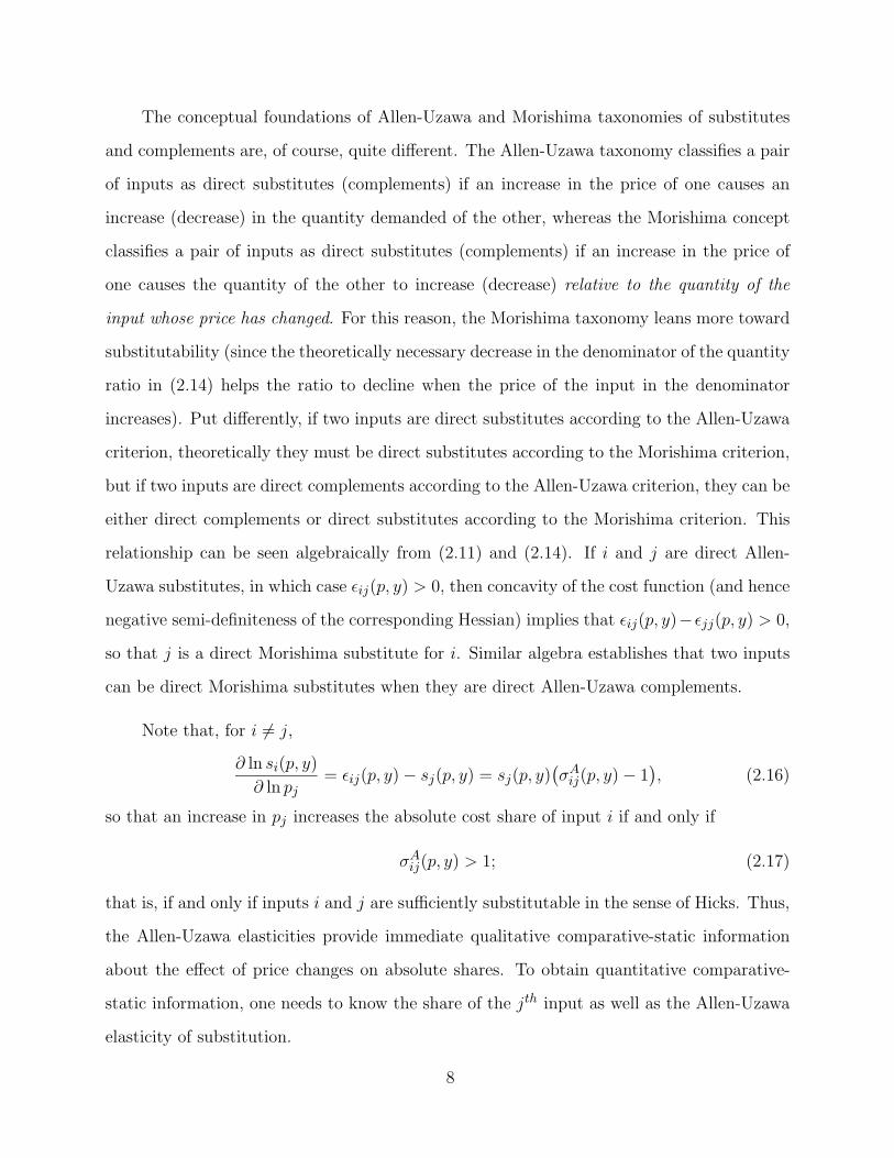
The conceptual foundations of Allen-Uzawa and Morishima taxonomies of substitutes
and complements are, of course, quite different. The Allen-Uzawa taxonomy classifies a pair
of inputs as direct substitutes (complements) if an increase in the price of one causes an
increase (decrease) in the quantity demanded of the other, whereas the Morishima concept
classifies a pair of inputs as direct substitutes (complements) if an increase in the price of
one causes the quantity of the other to increase (decrease) relative to the quantity of the
input whose price has changed. For this reason, the Morishima taxonomy leans more toward
substitutability (since the theoretically necessary decrease in the denominator of the quantity
ratio in (2.14) helps the ratio to decline when the price of the input in the denominator
increases). Put differently, if two inputs are direct substitutes according to the Allen-Uzawa
criterion, theoretically they must be direct substitutes according to the Morishima criterion,
but if two inputs are direct complements according to the Allen-Uzawa criterion, they can be
either direct complements or direct substitutes according to the Morishima criterion. This
relationship can be seen algebraically from (2.11) and (2.14). If i and j are direct Allen-
Uzawa substitutes, in which case εij(p, y) > 0, then concavity of the cost function (and hence
negative semi-definiteness of the corresponding Hessian) implies that εij(p, y)− εjj(p, y) > 0,
so that j is a direct Morishima substitute for i. Similar algebra establishes that two inputs
can be direct Morishima substitutes when they are direct Allen-Uzawa complements.
Note that, for i 6= j,
∂ ln si(p, y)
∂ ln pj= εij(p, y)− sj(p, y) = sj(p, y)
(σAij(p, y)− 1
), (2.16)
so that an increase in pj increases the absolute cost share of input i if and only if
σAij(p, y) > 1; (2.17)
that is, if and only if inputs i and j are sufficiently substitutable in the sense of Hicks. Thus,
the Allen-Uzawa elasticities provide immediate qualitative comparative-static information
about the effect of price changes on absolute shares. To obtain quantitative comparative-
static information, one needs to know the share of the jth input as well as the Allen-Uzawa
elasticity of substitution.
8

The Morishima elasticities immediately yield both qualitative and quantitative infor-
mation about the effect of price changes on relative input shares:
∂ ln(si(pi, y
)/sj(pi, y
))∂ ln(pj/pi)
= εij(p, y)− εjj(p, y)− 1 = σMij (p, y)− 1, (2.18)
where (with the use of zero-degree homogeneity of si in p) si(pi, y) := si(p, y) for all i. Thus,
an increase in pj increases the share of input i relative to input j if and only if
σMij (p, y) > 1; (2.19)
that is, if and only if inputs i and j are sufficiently substitutable in the sense of Morishima.
Moreover, the degree of departure of the Morishima elasticity from unity provides immediate
quantitative information about the effect on the relative factor shares.
2.3. Dual Elasticities of Substitution.
The (natural) dual to the Morishima elasticity of substitution (proposed by Blackorby
and Russell [1975, 1981]) is given by
∗σMij (x, y) : =∂ ln
(ρi(xi, y
) /ρj(xi, y
))∂ ln(xj/xi)
= xj
(Dij(x, y)
Di(x, y)− Djj(x, y)
Dj(x, y)
)= ∗ε ij(x, y)− ∗ε jj(x, y),
(2.20)
where xi is the (n−1)-dimensional vector of input quantity ratios with xi in the denominator
and
∗ε ij(x, y) =∂ ln ρi(x, y)
∂ ln xj(2.21)
is the (constant-output) elasticity of the shadow price of input i with respect to changes in
the quantity of input j. Analogously, Blackorby and Russell [1981] proposed the following
as the natural dual to the Allen-Uzawa elasticity:
∗σAij(x, y) =D(x, y)Dij(x, y)
Di(x, y)Dj(x, y)
=∗ε ij(x, y)∗s j(x, y)
,
(2.22)
9

where
∗s j(x, y) = ρj(x, y) · xj (2.23)
is the cost share of input j (assuming cost-minimizing behavior).
If ∗σAij(p, y) < 0 (that is, if increasing the jth quantity decreases the shadow price of
input i), we say that inputs i and j are dual Allen-Uzawa substitutes; if ∗σAij(p, y) > 0, they
are dual Allen-Uzawa (net) complements. Similarly, if σMij (p, y) < 0 (that is, if increasing the
jth quantity increases the shadow price of input i relative to the shadow price of input j), we
say that input j is a dual Morishima substitute for input i; if σMij (p, y) > 0, input j is a dual
Morishima complement to input i. Primal and dual substitutability and complementarity are
fundamentally different concepts; indeed, signs in these definitions of dual substitutability
and complementarity are reversed from those in the definitions of direct Allen-Uzawa and
Morishima substitutes and complements. Thus, if n = 2, the two inputs are necessarily
direct substitutes and dual complements.11
Interestingly, since the distance function is concave in x, and hence ∗ε jj(x, y) in (2.20)
is non-positive, the dual Morishima elasticity leans more toward dual complementarity than
does the dual Allen-Uzawa elasticity (in sharp contrast to the primal taxonomy). Similarly, if
two inputs are dual Allen-Uzawa complements, they must be dual Morishima complements,
whereas two inputs can be dual Allen-Uzawa substitutes but dual Morishima complements.
There exist, of course, dual comparative-static results linking factor cost shares and
elasticities of substitution.12 Consider first the effect of quantity changes on absolute shares
(for i 6= j):
∂ ln ∗s i(x, y)
∂ ln xj= ∗ε ij(x, y) = ∗σAij(x, y) ∗s(x, y), (2.24)
11 The direct Allen-Uzawa and Morishima elasticities are idential when n = 2, as are the dual Allen-Uzawaand Morishima elasticities.12 While shadow prices and dual elasticities are well defined even if the input requirement sets are not
convex, the comparative statics of income shares using these elasticities requires convexity (as well, of course,as price-taking, cost-minimizing behavior), which implies concavity of the distance function in x. By wayof contrast, convexity of input requirement sets is not required for the comparative statics of income sharesusing direct elasticities, since the cost function is necessarily concave in prices. See Russell [1997] for adiscussion of these issues.
10

so that an increase in xj increases the absolute share of input i if and only if
∗ε (x, y) > 0 (2.25)
or, equivalently,
∗σAij(x, y) > 0; (2.26)
that is, if and only if inputs i and j are dual Allen-Uzawa complements. Thus, the dual Allen-
Uzawa elasticities provide immediate qualitative comparative-static information about the
effect of quantity changes on (absolute) shares. To obtain quantitative comparative-static
information, one needs to know the share of the jth input as well as the dual Allen-Uzawa
elasticity of substitution. Of course, the (constant-output) dual elasticity ∗ε ij(x, y) yields the
same qualitative and quantitative comparative-static information.
Dual comparative-static information about relative income shares in the face of quantity
changes can be extracted from the dual Morishima elasticity concept:
∂ ln(si(xi, y
)/sj(xi, y
))∂ ln(xj/xi)
= ∗ε ij(x, y)− ∗ε jj(x, y)− 1 = ∗σMij (x, y)− 1, (2.27)
where (with the use of zero-degree homogeneity of ∗x in x) si(xi, y) := ∗s i(x, y). Thus, an
increase in xj increases the share of input i relative to input j if and only if
∗σMij (x, y) > 1; (2.28)
that is, if and only if inputs i and j are sufficiently complementary in terms of the dual Mor-
ishima elasticity. Moreover, the degree of departure from unity provides immediate quanti-
tative information about the effect on the relative factor share. Thus, the dual Morishima
elasticities provide immediate quantitative and qualitative comparative-static information
about the effect of quantity changes on relative shares.
11

2.4. Scalar-Output Dual Elasticities of Substitution.
An earlier literature (Hicks [1970] and Sato and Koizumi [1973]) analyzed duals to the
Allen elasticity under the assumptions of a single output (m = 1) and constant returns to
scale. The Hicksian “elasticity of complementarity” between inputs i and j is defined as
∗σHij (x, y) :=f(x)fij(x)
fi(x)fj(x), (2.29)
where subscripts on the production function f indicate differentiation with respect to the
indicated variable(s). The symmetry with the Allen elasticity of substitution (2.11) is ob-
vious. This formulation relies critically, however, on homogeneity of degree one (as well as
m = 1), as shown by the following theorem.
Theorem: Suppose m = 1. Then the Hicks elasticity of complementarity (2.29) is equivalent
to the dual Allen-Uzawa elasticity of substitution (2.22) if and only if the production function
is homogeneous of degree one (i.e., (2.3) holds).
Proof: Sufficiency is easily established by differentiating (2.3) and substituting the resulting
identities intof(x)fij(x)
fi(x)fj(x)=D(x, y)Dij(x, y)
Di(x, y)Dj(x, y). (2.30)
To prove necessity, differentiate the identity,
D(f(x), x
)= 1, (2.31)
with respect to xi and substitute the result into (2.30) to obtain
f(x)fij(x) =D(x, y)Dij(x, y)[
Dy(x, y)]2 . (2.32)
Now multiply both sides of (2.32) by xj and sum over j to arrive at
f(x)∑j
fij(x)xj =D(x, y)[Dy(x, y)
]2 ∑j
Dij(x, y) xj = 0, (2.33)
12

where the last identity follows from the first-degree homogeneity of D in x (and hence zero-
degree homogeneity of Di in x). This implies that∑j
fij(x)xj = 0, (2.34)
which in turn, by the converse of Euler’s theorem,13 implies that f is homogeneous of degree
one.
3. Empirical Implementation.
3.1. Specification of functional form.
Parametric application of the concepts in Section 2 requires specification of a cost
function or a distance function. We adopt translog specifications, incorporating technological
change (proxied by a time index t) of each:14
lnC(p, y, t) = α0 +n∑i=1
αi ln pi +m∑i=1
βi ln yi +1
2
n∑i=1
n∑j=1
αij ln pi ln pj
+1
2
m∑i=1
m∑j=1
βij ln yi ln yj +n∑i=1
m∑j=1
γij ln pi ln yj
+ θt +n∑i=1
νit ln pi +m∑i=1
τi t ln yi
(3.1)
and
lnD(x, y, t) = α0 +n∑i=1
αi ln xi +m∑i=1
βi ln yi +1
2
n∑i=1
n∑j=1
αij ln xi ln xj
+1
2
m∑i=1
m∑j=1
βij ln yi ln yj +n∑i=1
m∑j=1
γij ln xi ln yj
+ θt +n∑i=1
νit ln xi +m∑i=1
τit ln yi,
(3.2)
13 See, e.g., Simon and Blume [1994, pp. 672–3].14 We choose these two specifications because of their flexibility (in the sense of both Diewert [1971] and
Jorgenson and Lau [1975]). The two specifications represent different technologies; that is, the translog is notself-dual. Moreover, it is not possible to find closed-form duals to either of these specifications, unless theydegenerate to representations of a Cobb-Douglas technology (which is self-dual). Of course, the stochasticstructure is also quite different in the two specifications.
13

where the last three terms in each specification reflect technological change. The correspond-
ing systems of share equations are given by
si(p, y, t) =∂ lnC(p, y, t)
∂ ln pi= αi +
n∑j=1
αij ln pj +m∑j=1
γij ln yj + νit, i = 1, . . . , n, (3.3)
and
∗s i(x, y, t) =∂ lnD(x, y, t)
∂ ln xi= αi +
n∑j=1
αij ln xj +m∑j=1
γij ln yj + νit, i = 1, . . . , n. (3.4)
The homogeneity restrictions on C and D imply the following restrictions in each of these
two specifications:∑i
αi = 1 and∑i
αij =∑i
γij =∑i
νi = 0 ∀ j. (3.5)
The above specifications of the cost and distance functions impose no restrictions on
returns to scale. Constant returns to scale imposes the following additional restrictions on
(3.1) or on (3.2): ∑i
βi = 1 and∑j
βij =∑j
γij = 0 ∀ i. (3.6)
Thus, one tests for constant returns to scale by testing for these parametric restrictions.
3.2. Application: Resident and Non-Resident Workers in Switzerland.
We illustrate the application of the foregoing concepts using annual data on resident
and non-resident workers in Switzerland for the 1950–1986 time period.15 This data base
has only a single (aggregate) output, along with four inputs—resident labor, non-resident
labor, imports, and capital. Gross output and import figures are derived from the Swiss
National Income and Product Accounts. The quantity of labor is the product of total
employment and the average length of the work week. The quantity of capital is calculated
as the Tornqvist quantity index of structures and equipment. The income shares of labor
and capital are derived from the National Income and Product Accounts, and the prices of
15 We thank Ulrich Kohli for providing these data.
14

labor and capital are obtained by deflation. The resident-worker category comprises natives
as well as foreign workers who are residents of Switzerland. Nonresident workers are holders
of seasonal permits, annual permits, or transborder permits. We use a time trend with unit
annual increments for technological change.
Tables 1 and 2 contain estimates of the systems of share equations, (3.3) and (3.4),
respectively, under alternative assumptions about returns to scale.16 The subscripts of the
coefficients in the first column, L, N, M , K, and Y , represent resident labor, non-resident
labor, imports, capital, and output, respectively.
We first test for positive linear homogeneity of the production function under each of
these specifications. In each case, the critical value of the Wald test statistic for constant
returns to scale, under the null of γLY = γNY = γMY = γKY = 0, is 9.31. The Wald
statistic for the estimates of the systems (3.3) and (3.4) are 100.2 and 29.1, respectively;
thus, positive linear homogeneity is decisively rejected in each case. It appears, therefore, in
the light of the above Theorem, that the dual-elasticity concept suggested by Hicks [1970]
and Sato and Koizumi [1973] (and adopted by Kohli [1999]), which relies on constant returns
to scale, is inappropriate (at least in the case of the Kohli data set).
Tables 3 and 4 contain estimates of the direct Allen-Uzawa and Morishima elasticities
of substitution (equations (2.11) and (2.14)), and Tables 5 and 6 contain estimates of the
dual elasticities (equations (2.22) and (2.20)), all evaluated at the means of the variables
and under alternative assumptions about returns to scale.
16 Zellner’s SURE technique was used to estimate the systems of factor-share equations, and the capital-share equation was deleted for the estimation. Because of possibile simultaneous-equations bias, we alsoran three-stage least squares; the coefficients were substantially unchanged in each case. Hausman testsrejects the hypothesis of endogenity of input quantities in the estimation of the share equations in the directspecification and of endogenity of prices in the dual specification. Tests for concavity of the cost function(whence the system (3.3) is derived) were satisfied for 32 of the 37 observations. Concavity of the distancefunction (whence (3.4) is derived) was satisfied at 23 of the 37 observations. Concavity of the cost functionis a theoretical imperative. Concavity of the distance function is implied by convexity of input requirementsets L(y), but the distance function is well defined, as are the shadow price functions given by (2.10), even ifinput requirement sets are not convex. On the other hand, the comparative statics of income shares underperfectly competitive pricing of inputs, reflected in (2.24) and (2.27), require convexity of input requirementsets as does the estimation of the share equations (2.10) using price data.
15

Let us first evaluate the qualitative information in these tables. Recall that two factors
are classified as direct (Allen-Uzawa or Morishima) substitutes if the direct elasticity is
positive and as complements if it is negative, and the reverse is true for the dual elasticities.
Of course, the non-symmetry of the Morishima elasticities raises the possibility of ambiguities
in the Morishima taxonomy. Examination of the tables, however, reveals that there are only
two qualitative asymmetries, for capital and imports in the dual homogeneous case (Table
5) and for capital and nonresident labor in the dual non-homogeneous framework (Table 6),
and in each case one of the two elasticity estimates is statistically insignificant. Hence, it
is possible to construct an unambiguous taxonomy of (direct and dual) substitutability and
complementarity for the Morishima elasticities as well as the Allen elasticities (evaluated at
the means of the data). This taxonomy is summarized in Table 7, where S signifies (direct
or dual) substitutability and C signifies (direct or dual) complementarity.
The strongest priors exist for resident and non-resident labor, and, indeed, the two are
substitutes under either assumption about returns to scale, in either the primal or dual spec-
ification, and with respect to either elasticity definition.17 Thus, an increase in the number
of non-resident workers lowers the wage rate of resident workers, both absolutely and rela-
tively to the wage rate of non-resident workers. And an increase in the wage rate of resident
workers increases the demand for non-resident workers, both absolutely and relatively to the
demand for resident workers.
Some differences emerge with other pairs of inputs. First, regarding the assumption
about returns to scale, there are a couple of reversals using the direct Allen elasticity def-
inition and one reversal in the dual under both elasticity definitions. As the above test
indicates that the constant-returns-to-scale cost and distance functions are mispecified, we
would conclude that non-resident labor and imports are direct Allen-Uzawa substitutes and
that imports and capital are direct Allen-Uzawa complements. Similarly, we would conclude
that non-resident labor and capital are dual substitutes under either elasticity definition.
17 Cf. the finding of substitutability between immigrant and native workers by Grossman [1982].
16

Hence, an increase in the number of non-resident workers lowers the rental rate on capital,
both absolutely and relatively to the wage rate of non-resident workers.
It should be re-emphasized that contrasts in the classification of pairs as substitutes
or complements in the primal and the dual do not constitute any kind of theoretical or
econometric inconsistency: the direct and dual elasticities measure conceptually distinct
phenomena when there are more than two inputs.18 The direct elasticities measure the
effect on quantities of price changes whereas the dual elasticities measure the effect on prices
of changes in quantities.
Finally, regarding the difference in taxonomies induced by the two elasticity concepts,
it is clear that the direct Morishima elasticity concept is more conducive to substitutability
than the direct Allen-Uzawa elasticity, as shown theoretically in Section 2 above. In some
(direct elasticity) cases, pairs are classified as complements by the Allen elasticity concept
but as substitutes by the Morishima concept. Interestingly, however, there is no difference
in the classification scheme in the dual. Again, we wish to re-emphasize that there is no
theoretical or econometric reason why the two elasticity concepts should yield comparable
qualitative conclusion about substitutability/complementarity; they are measuring different
concepts, as discussed in Section 2 above.
To consider the quantitative elasticity results, we take note of the fact that the Allen-
Uzawa elasticity of substitution has no meaningful quantitative interpretation, as pointed out
by Blackorby and Russell [1975, 1989]. The size of the simple cross price elasticity εij(p, y)
is meaningful, but dividing by the share of input j, as in (2.11), to obtain the Allen-Uzawa
elasticity, σAij(p, y), undermines this quantitative content. Thus, to facilitate consideration
of quantitative comparative statics, we list the price elasticities and their duals, defined by
(2.12) and (2.21) and evaluated at the means of the data, in Table 8. Of course, these
elasticities are non-symmetric.
18 As noted earlier, they require different theoretical and stochastic specifications of the technology as well.
17

Let us focus now on the quantitative relationships between the two types of labor under
the (preferred) non-homogeneous specification of the technology. The estimated cross price
elasticities in Table 8 indicate that a 1-percent increase in the wage rate of non-resident
workers would increase the employment of resident labor by 0.3 percent (at the means of
the data), whereas a 1-percent increase in the wage rate of resident labor would increase
the employment of non-resident labor by 1.8 percent.19 Table 3 indicates that a 1-percent
increase in the price of non-resident labor would increase the quantity ratio of resident labor
to non-resident labor by 1.7 percent, while a 1-percent increase in the wage rate of resident
labor would increase the quantity ratio of non-resident to resident labor by 2.5 percent.20
The dual price elasticity estimates in Table 8 suggest that a 1-percent increase in the
number of nonresident workers would lower the wage rate of resident workers by 0.1 percent,
while a 1-percent increase in the number of resident workers would lower the wage rate of
non-resident workers by 0.6 percent. From Table 6, it appears that a 1-percent increase in
the number of non-resident workers would lower the relative wage rate (of non-resident to
resident workers) by just 0.1 percent, while a 1-percent increase in the number of resident
workers would lower the relative wage rate (of resident to non-resident workers) by 0.5
percent.
The estimated direct Allen-Uzawa elasticity of substitution does provide immediate
qualitative information about absolute shares, as reflected in (2.16). Thus, the elasticity
of 4.3 in Table 4 indicates that the share of either type of labor input is enhanced by an
increase in the wage rate of the other labor type. Similarly, from (2.24) and Table 6, we see
from the negative sign of the dual Allen-Uzawa elasticity that an increase in the quantity
of either input decreases the absolute share of the other labor input. Equations (2.22) and
(2.27), along with the estimates of Morishima elasticities in Tables 4 and 6, provide both
19 It is interesting to note here that, under the (apparently mispecified) homogeneous technology, a 1-percent increase in the wage rate of resident labor would increase the employment of non-resident labor bya whopping 4.4 percent, an estimate that strains credibility.20 Again, note that under the mispecified homogeneous technology, a 1-percent change in a wage rate
generates an estimated 3-percent or 6-percent change in the quantity ratio, again challenging our intuition.
18
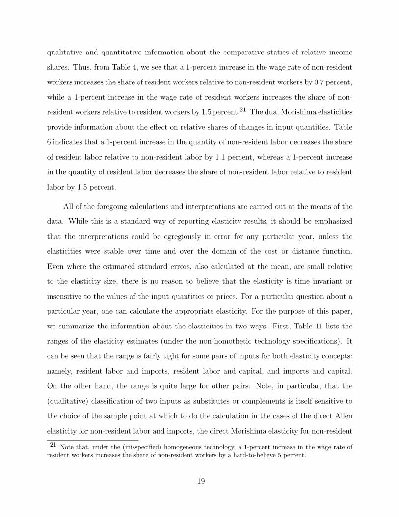
qualitative and quantitative information about the comparative statics of relative income
shares. Thus, from Table 4, we see that a 1-percent increase in the wage rate of non-resident
workers increases the share of resident workers relative to non-resident workers by 0.7 percent,
while a 1-percent increase in the wage rate of resident workers increases the share of non-
resident workers relative to resident workers by 1.5 percent.21 The dual Morishima elasticities
provide information about the effect on relative shares of changes in input quantities. Table
6 indicates that a 1-percent increase in the quantity of non-resident labor decreases the share
of resident labor relative to non-resident labor by 1.1 percent, whereas a 1-percent increase
in the quantity of resident labor decreases the share of non-resident labor relative to resident
labor by 1.5 percent.
All of the foregoing calculations and interpretations are carried out at the means of the
data. While this is a standard way of reporting elasticity results, it should be emphasized
that the interpretations could be egregiously in error for any particular year, unless the
elasticities were stable over time and over the domain of the cost or distance function.
Even where the estimated standard errors, also calculated at the mean, are small relative
to the elasticity size, there is no reason to believe that the elasticity is time invariant or
insensitive to the values of the input quantities or prices. For a particular question about a
particular year, one can calculate the appropriate elasticity. For the purpose of this paper,
we summarize the information about the elasticities in two ways. First, Table 11 lists the
ranges of the elasticity estimates (under the non-homothetic technology specifications). It
can be seen that the range is fairly tight for some pairs of inputs for both elasticity concepts:
namely, resident labor and imports, resident labor and capital, and imports and capital.
On the other hand, the range is quite large for other pairs. Note, in particular, that the
(qualitative) classification of two inputs as substitutes or complements is itself sensitive to
the choice of the sample point at which to do the calculation in the cases of the direct Allen
elasticity for non-resident labor and imports, the direct Morishima elasticity for non-resident
21 Note that, under the (misspecified) homogeneous technology, a 1-percent increase in the wage rate ofresident workers increases the share of non-resident workers by a hard-to-believe 5 percent.
19

labor and capital, and the dual Morishima elasticity for resident and non-resident labor and
for non-resident labor and imports.
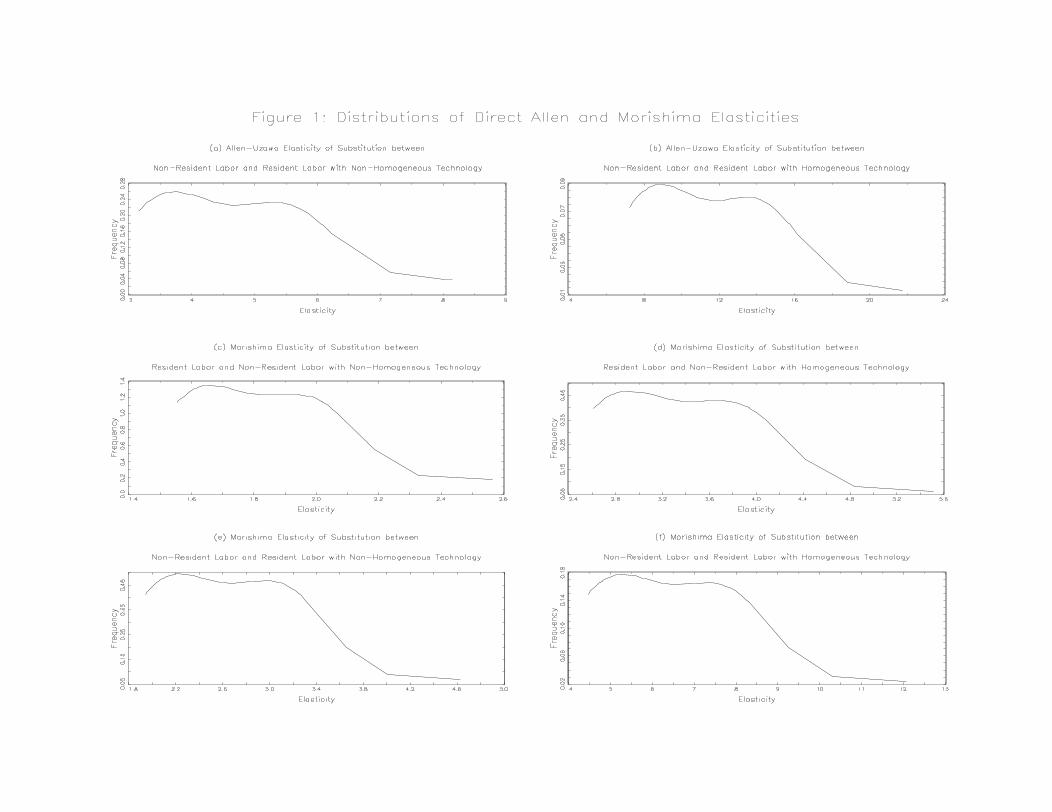
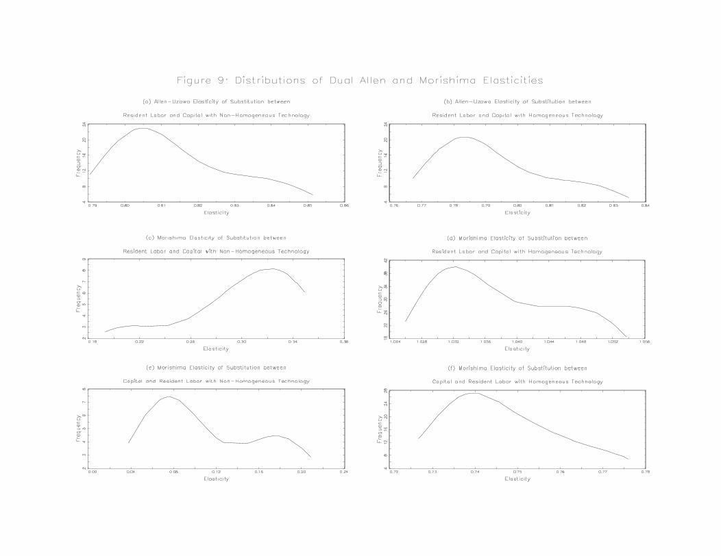
A second way to summarize the information about the elasticity values over the entire
sample space is to plot frequency distributions. We have constructed nonparametric, kernel-
based density estimates of the distributions of each of the elasticities (essentially “smoothed”
histograms of elasticity values) over the entire sample (numbering 72 distributions).22 [These
distributions are attached as a not-for-publication appendix to this draft for the convenience
of the editor and referees. They will be made available online.] While many of the distri-
butions look radically different for the homogeneous and non-homogeneous cases, some look
similar. This raises the possibility that, even though the hypothesis of constant returns to
scale is easy to reject (at least for this data set), the apparent mispecification might have
little effect on estimated elasticity values and hence on qualitative and quantitative com-
parative statics of price, quantities, and income shares. Using some recent developments in
nonparametric methods, we can test this hypothesis formally by testing for the difference
between the elasticity distributions under homogeneous vs. non-homogeneous technologies.
In particular, Fan and Ullah [1999] have proposed a nonparametric (time series) test for the
comparison of two unknown distributions, say f and g—that is, a test of the null hypothesis,
H0 : f(x) = g(x) for all x, against the alternative, H1 : f(x) 6= g(x) for some x.23 Tables
10 and 11 contain the results of carrying out these tests. The hypothesis that the two dis-
tributions are identical is rejected in every case but one: the direct Allen elasticity between
non-resident labor and capital. Thus, it is safe to say that the mispecification of constant
returns to scale, required for the Hicks [1970] and Sato-Koizumi [1973] dual elasticity concept
(see the Theorem in Section 2.4), results in serious errors in elasticity estimates and hence
in serious errors in the comparative statics of prices, quantities, and income shares.
22 See the Appendix for the particulars.23 See the Appendix for an exact description of the test statistic.
20

4. Summary and Concluding Remarks.
In this paper we have argued that different elasticity of substitution concepts—direct and
dual Allen-Uzawa elasticities and direct and dual Morishima elasticities—must be used to
answer different questions about substitutability among multiple (more than two) factors of
production. To assess the effects of price changes, direct elasticities should be used; to assess
the effects of quantity changes, dual elasticities should be used. But there is a tendency
in the literature to rely on a single elasticity concept regardless of the question: typically
the (direct) Allen-Uzawa elasticity but increasingly the (direct) Morishima elasticity. Hicks
[1970] did formulate a dual concept, the elasticity of complementarity, under the assumptions
of a single output and constant returns to scale. Blackorby and Russell [1981] proposed a
generalization of the Hicks notion, a dual Allen-Uzawa elasticity, to encompass multiple-
output and non-homothetic technologies. This concept runs parallel to the formulation of
the dual Morishima elasticity by Blackorby and Russell [1981].
This generalization of Hicks elasticity might be important not only because of the
increasing use of data bases with multiple outputs, but also because constant returns to scale
is not difficult to reject when there are more than two factors of production. Indeed, using a
data base on the Swiss labor market, we definitively reject the hypothesis of homotheticity
under two different specifications of the technology: a translog cost function and a translog
distance function. Moreover, maintaining a non-homogeneous translog (cost or distance
function) technology, we find that mispecification of the technology as homogeneous of degree
one results in statistically significant errors in the estimated elasticities of substitution and
hence in assessments of the effects on input demands, prices, or shares of changes in quantities
or prices.
21
APPENDIX
Each of the distributions in Figures 1–12 is a kernel-based estimate of a density function,
f(·), of a random variable x, based on the standard normal kernel function and optimal
bandwidth:
f(x) =1
nh
J∑j=1
k
(xj − xh
),
where∫∞−∞ k(ψ)dψ = 1 and ψ = (xj − x)/h. In this construction, h is the optimal window
width, which is a function of the sample size n and goes to zero as n→∞. We assume that
k is a symmetric standard normal density function, with non-negative images. See Pagan
and Ullah (1999) for details.
The statistic used to test for the difference between two distributions, predicated on the
integrated-square-error metric on a space of density functions, I(f, g) =∫x
(f(x)−g(x)
)2dx,
is
T =nh1/2I
σ∼ N(0, 1), (A.1)
where
I =1
n2h
n∑i=1
(i6=j)
n∑j=1
[k
(xi − xjh
)+ k
(yi − yjh
)− 2k
(yi − xjh
)− k(xi − yjh
)](A.2)
and
σ2 =2
n2h
n∑i=1
n∑j=1
[k
(xi − xjh
)+ k
(yi − yjh
)+ 2k
(xi − yjh
)]∫k2(Ψ)dψ. (A.3)
As shown by Fan and Ullah [1999], the test statistic asymptotically goes to the standard
normal, but the sample in our study is only 37 years. Thus, we do a bootstrap approximation
with 2000 replications to find the critical values for the statistic at the 5-percent and 1-percent
levels of significance (see Tables 10–13).
22

REFERENCES
Allen, R. G. D. [1938], Mathematical Analysis for Economists, London: Macmillan.
Allen, R. G. D., and J. R. Hicks [1934], “A Reconsideration of the Theory of Value, II,”Economica 1, N.S. 196–219.
Barnett, W. M., D. Fisher, and A. Serletis [1992], “Consumer Theory and the Demand forMoney,” Journal of Economic Literature 30: 2086–2119.
Berndt, E. R., and D. O. Wood [1975], “Technology, Prices, and the Derived Demand forEnergy,” Review of Economics and Statistics 57: 376–384.
Blackorby, C., and R. R. Russell [1975], “The Partial Elasticity of Substitution,” DiscussionPaper No. 75-1, Department of Economics, University of California, San Diego.
Blackorby, C., and R. R. Russell [1981], “The Morishima Elasticity of Substitution: Symme-try, Constancy, Separability, and Its Relationship to the Hicks and Allen Elasticities,”Review of Economic Studies 48: 147–158.
Blackorby, C., and R. R. Russell [1989], “Will the Real Elasticity of Substitution PleaseStand Up? (A Comparison of the Allen/Uzawa and Morishima Elasticities),” AmericanEconomic Review 79: 882–888.
Borjas, G. J. [1994], “The Economics of Immigration,” Journal of Economic Literature 32:1667–1717.
Borjas, G. J., R. B. Freeman, and L. F. Katz [1992], “On the Labor Market Effects ofImmigration and Trade,” in G. Borjas and R. Freeman (eds.), Immigration and TheWork Force, Chicago: University of Chicago Press, 213-44.
Borjas, G. J., R. B. Freeman, and L. F. Katz [1996], “Searching for the Effect of Immigrationon the Labor Market,” AEA Papers and Proceedings 86: 246–251.
Davis, G. C., and J. Gauger [1996], “Measuring Substitution in Monetary-Asset DemandSystems, Journal of Business and Economic Statistics 14: 203–209.
de la Grandville, O. [1997], “Curvature and the Elasticity of Substitution: Straightening ItOut,” Journal of Economics 66: 23–34.
Diewert, W. E. [1971], “An Application of the Shephard Duality Theorem: A GeneralizedLeontief Production Function,” Journal of Political Economy 79: 481-507.
Diewert, W. E. [1974], “Applications of Duality Theory,” in Frontiers of QuantitativeEconomics , Vol. 2, edited by M. Intriligator and D. Kendrick, Amsterdam: North-Holland.
Diewert, W. E. [1982], “Duality Approaches to Microeconomic Theory,” in Handbook ofMathematical Economics , Vol. II, edited by K. Arrow and M. Intriligator, New York:North-Holland.
23

Ewis, N., and D. Fischer [1984], “The Translog Utility Function and the Demand for Moneyin the United States,” Journal of Money, Credit, and Banking 16: 34–52.
Fan, Y., and A. Ullah [1999], “On Goodness-of-fit Tests for Weakly Dependent ProcessesUsing Kernel Method,” Journal of Nonparametric Statistics 11: 337–360.
Fare, R., and S. Grosskopf [1994], Cost and Revenue Constrained Production, Berlin:Springer-Verlag.
Fare, R., and D. Primont [1995], Multi-Output Production and Duality: Theory and Appli-cations, Boston: Kluwer Academic Press
Flaussig, A. R. [1997], “The Consumer Consumption Conundrum: An Explanation,” Journalof Money, Credit, and Banking 29: 177–191.
Fuss, M., and D. McFadden (eds.) [1978], Production Economics; A Dual Approach to Theoryand Applications , Amsterdam: North-Holland.
Griliches, Z. [1969], “Capital-Skill Complementarity,” Review of Economic and Statistics 51:465–468.
Grossman, J. [1982], “The Substitutability of Natives and Immigrants in Production,” Reviewof Economics and Statistics 64: 596–603.
Hicks, J. R. [1932], Theory of Wages, London: Macmillan.
Hicks, J. R. [1970], “Elasticity of Substitution Again: Substitutes and Complements,” OxfordEconomic Papers 22: 289–296.
Johnson, G. E. 1970], “The Demand for Labor by Educational Category,” Southern EconomicJournal 37: 190–204.
Jorgenson, D. C., and L. J. Lau [1975], “Transcendental Logarithmic Utility Functions,”American Economic Review , 65: 367-383.
Klump, R., and O. de la Grandville [2000], “Economic Growth and the Elasticity ofSubstitution: Two Theorems and Some Suggestions,” American Economic Review 90:282–291.
Kohli, U. [1999], “Trade and Migration: A Production Theory Approach,” in Migration: TheControversies and the Evidence, edited by R. Faini, J. de Melo, and K. F. Zimmermann,Cambridge: Cambridge University Press.
Kugler, P., U. Muller, and G. Sheldon [1989], “Non-Neutral Technical Change, Capital,White-Collar and Blue-Collar Labor,” Economics Letters 31: 91–94.
McFadden, D. [1963], “Constant Elasticity of Substitution Production Functions,” Reviewof Economic Studies 30: 73–83.
Morishima, M. [1967], “A Few Suggestions on the Theory of Elasticity” (in Japanese), KeizaiHyoron (Economic Review) 16: 144–150.
24

Pagan, A., and A. Ullah, Nonparametric Econometics. London: Cambridge University Press,1999.
Russell, R. R. [1997], “Distance Functions in Consumer and Producer Theory,” Essay 1 inIndex Number Theory: Essays in Honor of Sten Malmquist, Boston: Kluwer AcademicPublishers, 7–90 .
Sato, R., and T. Koizumi [1973], “On the Elasticities of Substitution and Complementarity,”Oxford Economic Papers 25: 44–56.
Simon, C. P., and L. Blume [1994], Mathematics for Economists, New York: Norton.
Thompson, P., and T. G. Taylor [1995], “The Capital-Energy Substitutability Debate: ANew Look,” Review of Economics and Statistics 77: 565–569.
Uzawa, H. [1962], “Production Functions with Constant Elasticities of Substitution,” Reviewof Economic Studies 30: 291–299.
Welch, F. [1970], “Education in Production,” Journal of Political Economy 78: 35–59.
25

Table 1: Estimated Coefficients of the Translog Cost Function
(Standard error in parentheses)
CoefficientsHomogeneousTechnology
Non-HomogeneousTechnology
αL
0.433(0.008)
3.469(0.405)
α N
0.045(0.004)
-1.556(0.229)
α M
0.309(0.004)
0.024(0.343)
αK
-0.787(0.002)
1.937(0.187)
α LL
-0.424(0.065)
-0.051(0.059)
α LN
0.258(0.038)
0.089(0.034)
α LM
0.078(0.032)
-0.023(0.041)
α LK
0.088(0.113)
-0.015(0.110)
α NN
-0.101(0.029)
-0.035(0.025)
α NM
-0.101(0.022)
-0.012(0.025)
α NK
-0.056(0.07)
-0.042(0.125)
α MM
0.081(0.029)
0.033(0.045)
α MK
-0.058(0.067)
0.002(0.105)
α KK
-0.026(0.069)
0.055(0.083)
Lv 0.007(0.002)
0.002(0.001)
Nv -0.008(0.001)
-0.005(0.001)
Mv 0.003(0.001)
0.004(0.001)
Kv -0.002(0.005)
-0.001(0.001)
γ LY
-0.248(0.033)
γ NY
0.131(0.019)
γ MY
0.023(0.028)
γ KY
0.094(0.065)

Table 2: Estimated Coefficients of the Translog Distance Function
(Standard error in parentheses)
CoefficientsHomogeneousTechnology
Non-HomogeneousTechnology
αL
0.291(0.007)
0.431(0.034)
α N
0.156(0.005)
0.146(0.017)
α M
0.27(0.009)
0.275(0.033)
αK
0.283(0.01)
0.148(0.02)
α LL
0.070(0.009)
0.084(0.011)
α LN
-0.068(0.005)
-0.068(0.006)
α LM
-0.021(0.01)
0.002(0.01)
α LK
-0.02(0.01)
-0.018(0.04)
α NN
0.039(0.003)
0.039(0.004)
α NM
-0.004(0.006)
0.01(0.006)
α NK
0.033(0.01)
0.019(0.01)
α MM
0.11(0.017)
0.105(0.016)
α MK
-0.085(0.03)
-0.118(0.02)
α KK
0.138(0.02)
0.117(0.02)
Lv -0.0002(0.001)
-0.001(0.001)
Nv -0.001(0.0004)
-0.002(0.0005)
Mv -0.001(0.001)
0.001(0.0009)
Kv 0.002(0.001)
0.002(0.002)
γ LY
-0.102(0.23)
γ NY
0.004(0.011)
γ MY
0.001(0.023)
γ KY
-0.097(0.232)

Table 3: Direct Elasticities of Substitution: Homogeneous Technology
(Standard errors in parentheses)
Allen-Uzawa Elasticity of Substitution Morishima Elasticity of Substitution
L N M K L N M K
L -3.72(0.619)
10.44(3.903)
1.66(0.067)
1.89(0.085)
3.15(2.009)
0.89(0.082)
1.32(0.221)
N -38.41(44.82)
-4.67(3.317)
-2.73(2.089
6.00(0.771)
-0.87(0.813)
0.24(0.811)
M -1.54(0.132)
0.11(0.053)
2.28(0.035)
2.18(0.822)
0.90(0.18)
K -3.78(0.256)
2.38(0.022)
2.30(0.455)
0.46(0.014)
Table 4: Direct Elasticities of Substitution: Non-Homogeneous Technology
(Standard errors in parentheses)
Allen-Uzawa Elasticity of Substitution Morishima Elasticity of Substitution
L N M K L N M K
L -1.65(0.031)
4.26(0.404)
0.81(0.027)
0.85(0.007)
1.74(0.195)
0.83(0.002)
0.73(0.017)
N -22.69(0.004)
0.33(0.002)
-1.8(0.064)
2.50(0.002)
0.70(0.001)
0.11(0.002)
M -2.16(0.014)
-0.81(0.009)
1.04(0.016)
1.48(0.007)
0.34(0.008)
K -2.28(0.122)
1.06(0.007)
1.35(0.040)
0.38(0.037)

Table 5: Dual Elasticities of Substitution: Homogeneous Technology
(Standard errors in parentheses)
Dual Allen-UzawaElasticity of Substitution
Dual MorishimaElasticity of Substitution
L N M K L N M K
L -0.41(0.02)
-1.49(0.26)
0.82(0.03)
0.80(0.01)
-0.12(0.126)
0.32(0.256)
0.23(0.016)
N 0.33(0.99)
0.78(0.01)
0.80(0.06)
-0.46(0.028)
0.31(0.025)
0.23(0.024)
M -0.33(0.01)
-0.32(0.01)
0.52(0.015)
0.15(0.016)
-0.04(0.001)
K -0.17(0.03)
0.51(0.034)
0.03(0.015)
0.003(0.007)
Table 6: Dual Elasticities of Substitution: Non-Homogeneous Technology
(Standard errors in parentheses)
Dual Allen-UzawaElasticity of Substitution
Dual MorishimaElasticity of Substitution
L N M K L N M K
L -0.38(0.031)
-1.50(0.027)
1.02(0.027)
0.82(0.007)
-0.08(0.195)
0.51(0.002)
0.21(0.017)
N -0.32(0.004)
1.55(0.002)
-0.28(0.064)
-0.47(0.002)
0.15(0.001)
-0.04(0.002)
M -0.81(0.014)
-0.82(0.009)
0.59(0.008)
0.12(0.007)
-0.17(0.001)
K -0.10(0.02)
0.51(0.036)
0.003(0.037)
-0.003(0.037)
Table 7: Taxonomy for Substitutes and Complements
Direct DualHomogeneous
TechnologyNon-
HomogeneousTechnology
HomogeneousTechnology
Non-HomogeneousTechnology
AES MES AES MES AES MES AES MES
LN S S S S S S S S
LM S S S S C C C C
LK S S S S C C C C
NM C S S S C C C C
NK C S C S C C S S
MK S S C S S S S S

Table 8: Price and Quantity Elasticities (ε ij and ∗ε ij )
Direct Price Elasticity: Homogeneous Technology
L N M K
L -1.577 0.674 0.463 0.44
N 4.423 -2.5 -1.286 -0.636
M 0.703 -0.297 -0.431 0.025
K 0.802 -0.176 0.030 -0.879
Direct Price Elasticity: Non-Homogeneous Technology
L N M K
L -0.697 0.275 0.225 0.197
N 1.803 -1.477 0.093 -0.418
M 0.341 0.022 -0.603 0.240
K 0.359 -0.116 0.288 -0.531
Dual Quantity Elasticity: Homogeneous Technology
L N M K
L -0.411 -0.096 0.230 0.185
N -0.631 -0.33 0.217 -0.279
M 0.348 0.050 -0.327 -0.072
K 0.338 -0.077 -0.086 -0.853
Dual Quantity Elasticity: Non-Homogeneous Technology
L N M K
L -0.614 -0.096 0.284 0.19
N -0.631 -0.33 0.434 0.527
M 0.431 0.1 -0.345 -0.190
K 0.346 0.146 -0.228 -0.105

Table 9: Range for the Direct and Dual Elasticity
DIRECT DUALNon-Homogeneous Technology Non-Homogeneous Technology
AES MES AES MESMin Max Min Max Min Max Min Max
LN 3.15 8.15 1.56 2.56 -4.46 -0.64 -0.68 0.47
NL 1.94 4.63 -1.86 0.16LM 0.78 0.84 0.81 0.85 1.01 1.02 0.55 0.69ML 1.00 1.06 0.78 0.84LK 0.83 0.88 0.81 0.85 0.79 0.85 0.19 0.35KL 1.04 1.08 0.04 0.21
NM -0.96 0.61 0.39 0.77 1.32 2.63 -0.5 0.68
MN 1.27 2.34 -0.5 0.68
NK -6.32 -0.59 -0.91 0.39 1.72 4.31 0.52 1.11
MK 1.03 1.04 0.73 0.79 -0.64 -0.8 -0.16 -0.03

Table 10: Distribution Hypothesis Test Between Homogeneous and Non-Homogeneous Direct Allen Elasticity
Test Statistic 5% Significance Level 1% Significance Level
LowerCriticalValue
UpperCriticalValue
LowerCriticalValue
UpperCriticalValue
LN 0.402 0.1534 0.2292 0.1402 0.2439 Reject
ML 27.56 0.0024 0.0035 0.0023 0.0036 Reject
MK 330.49 0.0002 0.0004 0.0002 0.0004 Reject
NK 0.081 0.0426 0.0913 0.0396 0.1062 Fail to Reject
NM 1.67 0.0411 0.0918 0.0348 0.0988 Reject
Table 11: Distribution Hypothesis Test Between Homogeneous and Non-Homogeneous Direct Morishima Elasticity
TestStatistic
5% Level of Significance 1% Level ofSignificance
LowerCriticalValue
UpperCriticalValue
LowerCriticalValue
UpperCriticalValue
LN 2.19 0.0295 0.0511 0.0269 0.0546 Reject
NL 0.802 0.0792 0.1300 0.0723 0.1381 Reject
MK 30.78 0.0023 0.0034 0.0021 0.0036 Reject
KM 51.74 0.0013 0.0021 0.0012 0.0036 Reject
ML 39.83 0.0017 0.0028 0.0015 0.0031 Reject
LM 50.97 0.0011 0.0018 0.001 0.0018 Reject
NK 0.324 0.0066 0.0167 0.0057 0.0182 Reject
KN 1.762 0.0271 0.0461 0.0251 0.0495 Reject
MN 1.24 0.0207 0.0340 0.0192 0.0364 Reject
NM 6.06 0.0107 0.0206 0.0097 0.0221 Reject

Table 12: Distribution Test for Allen Dual Elasticity
TestStatistic
5% Significance Level 1% Significance Level
LowerCriticalValue
Upper CriticalValue
LowerCritical Value
UpperCriticalValue
NM 5.00 0.0134 0.0311 0.0117 0.0332 RejectNL 0.4 0.1498 0.2287 0.1360 0.2439 RejectLK 14.38 0.0007 0.0019 0.0007 0.0023 RejectNK 0.81 0.0078 0.0197 0.0068 0.0236 RejectMK 7.78 0.0089 0.0161 0.0076 0.0175 RejectML 316.98 0.0002 0.0003 0.0002 0.0003 Reject
Table 13: Distribution Hypothesis Test for Dual Morishima Elasticity
TestStatistic
5% Level of Significance 1% Level of Significance
LowerCriticalValue
UpperCriticalValue
Lower CriticalValue
UpperCriticalValue
NM 12.42 0.0057 0.0115 0.0042 0.0122 RejectMN 0.03 0.0006 0.0016 0.0005 0.0019 RejectLN 2.19 0.0286 0.0509 0.0261 0.0541 RejectNL 0.8 0.0766 0.1296 0.0697 0.1378 RejectLK 65.49 0.0011 0.0016 0.001 0.0017 RejectKL 41.2 0.0017 0.0025 0.0015 0.0027 RejectNK 1.94 0.007 0.0159 0.0061 0.0177 RejectKN 0.43 0.0078 0.0197 0.0068 0.0236 RejectMK 16.03 0.0038 0.0051 0.0035 0.0054 RejectKM 23.69 0.0026 0.0044 0.0023 0.0047 RejectML 37.18 0.0017 0.0021 0.0016 0.0022 RejectLM 9.8 0.0027 0.0038 0.0026 0.004 RejectNK 1.94 0.007 0.0159 0.0061 0.0177 RejectKN 0.43 0.0078 0.0197 0.0068 0.0236 Reject