1

STRUCTURED MARKETS: Derivative Markets, Risk Management, and Actuarial Methods

Binyomin B. Brodsky

2

BINYOMIN B. BRODSKY

SENIOR RESEARCH PROJECT IN MATHEMATICS - MAT 493

IN CONJUNCTION WITH

PROFESSOR DR. BASIL RABINOWITZ

HEAD OF ACTUARIAL DEPARTMENT

TOURO COLLEGE

LANDER COLLEGE OF ARTS AND SCIENCES

BROOKLYN, NY

JANUARY 2017

3

CONTENTS

1. ABSTRACT --------------------------------------------------------------------------------------- 4

1.1. An introduction to Derivatives ------------------------------------------------------------ 5

2. OPTION POSITIONS AND STRATEGIES ------------------------------------------------- 6

2.1. An introduction to Forwards and Options ----------------------------------------------- 6

2.2. Insurance, Hedging, and other strategies ------------------------------------------------- 8

2.3. An introduction to Risk Management ---------------------------------------------------- 10

3. FORWARDS, FUTURES, AND SWAPS ---------------------------------------------------- 12

3.1. Financial Forwards and Futures ----------------------------------------------------------- 12

3.2. Currency Forwards, And Futures --------------------------------------------------------- 17

3.3. Eurodollar Futures -------------------------------------------------------------------------- 19

3.4. Commodity Forwards and Futures -------------------------------------------------------- 20

3.5. Interest Rate Forwards and Futures ------------------------------------------------------- 22

3.6. Commodity and Interest Rate Swaps ----------------------------------------------------- 24

4. OPTION THEORIES AND PRICING MODELS ------------------------------------------- 28

4.1. Parity ------------------------------------------------------------------------------------------ 28

4.2. Binomial Option Pricing ------------------------------------------------------------------- 33

4.3. Lognormal Distributions for Stock Prices ----------------------------------------------- 36

4.4. Black Scholes -------------------------------------------------------------------------------- 39

5. INSURANCE AND RISK MANAGEMENT STRATEGIES ----------------------------- 41

5.1. Premiums ------------------------------------------------------------------------------------- 41

5.2. Deductibles ----------------------------------------------------------------------------------- 42

5.3. Investment Strategies And Asset Liability Management ------------------------------ 46

5.4. Risk assumptions and classes -------------------------------------------------------------- 49

6. CONCLUSION ----------------------------------------------------------------------------------- 52

7. Bibliography-Works Cited ---------------------------------------------------------------------- 53

STRUCTURED MARKETS

4

1. ABSTRACT

Structured Markets is so titled because it attempts to research the structure of both

the derivative markets and insurance principles, to consider, hypothesize, and

discuss alternative measures of consideration that can be taken by investors with

respect to loss and risk distributions.

We begin with an introduction to the financial derivatives markets, followed by

general option positions and strategies. We expand on the topic of option markets,

and explain their use in the context of risk management and where they may differ

from insurance. We consider various financial instruments such as forwards,

futures, swaps, and discuss how these instruments are constructed, with respect to

global financial markets, commodities, currencies, and interest rates. Finally, we

examine and discuss insurance features such as premiums, and deductibles, and

explain their relevancy to investments, and asset liability management. We

conclude the paper with some general remarks on risk assumptions and classes.

Our discussions are theoretically relevant to various different industries and can

therefore be thought of as all-inclusive. For the purposes of our discussion, we

refrain from choosing some specific industry, or asset portfolio, since this would

not affect any measure of pertinence, and would differ only with regard to

circumstantial applicability. An industry varies from another only with respect to

its particular key performance indicator(s) and its inherent nature(s) of risk; but

remains identically equivalent with respect to the constitution of the strategic

factors involved in its data analytics and performance.

5

1.1 An Introduction To Derivatives

Financial instruments are the essential backbones of all financial institutions, and

among these financial instruments are the derivative markets. Derivative markets

can include, but are not limited to, puts, call, forwards, futures, options, and swaps.

These instruments have numerous characteristics, including their financial

structure, and how they can be used to strategically implement procedures for

financial optimization. There can be many advantages to investing in derivatives as

opposed to investing in outright ownership of a specific asset or index, including

tax reductions, and lower transaction costs.

Clearly, there may be numerous differences between investing in derivatives and

investing in an underlying asset. One such distinction is that investing in

derivatives is generally a less costly investment, being that it can only be exercised

at a particular performance indicator, and in many cases, actually expire

unexercised.

Another distinction is that an investor who holds a position in derivatives is

generally concerned with optimizing his or her strategies and hedging techniques,

and can therefore becomes more fixated on long term and out of the money

positions. An investor in assets or indexes, on the other hand, may be more focused

on day to day trading, and in the money action. This is an important distinction.

Because derivatives are more heavily involved in positions that lie outside the

money, they also afford their investors the time to be able to change a position, and

thereby dramatically defer the risk exposure of these assets.

6

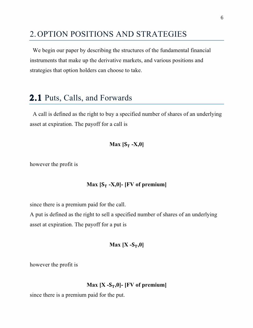
2. OPTION POSITIONS AND STRATEGIES

We begin our paper by describing the structures of the fundamental financial

instruments that make up the derivative markets, and various positions and

strategies that option holders can choose to take.

2.1 Puts, Calls, and Forwards

A call is defined as the right to buy a specified number of shares of an underlying

asset at expiration. The payoff for a call is

Max [𝐒𝐓 -X,0]

however the profit is

Max [𝐒𝐓 -X,0]- [FV of premium]

since there is a premium paid for the call.

A put is defined as the right to sell a specified number of shares of an underlying

asset at expiration. The payoff for a put is

Max [X -𝐒𝐓,0]

however the profit is

Max [X -𝐒𝐓,0]- [FV of premium]

since there is a premium paid for the put.

7

A seller of these derivatives would have the corresponding negative payoffs and

profits for both of these positions, and would be expressed as

-{Max [𝐒𝐓 -X,0]}

-{Max [𝐒𝐓-X,0]- [FV of premium]}

-{Max [X -𝐒𝐓,0]}

-{Max [X -𝐒𝐓,0]- [FV of premium]}

for calls and puts respectively.

Forwards are defined as an agreement to the purchase of an asset at a later point

in time at an agreed upon price and have equal profits and payoffs which are

𝐒𝐓 − 𝐅𝟎,𝐓

for a long position in the forward, and

𝐅𝟎,𝐓 − 𝐒𝐓

8

for a short position in the forward. We will have more to say about forwards later.

2 .2 Insurance, Hedging, and Option Strategies

We will proceed with some examples of option strategies that have insurance and

risk management features which are created using calls, puts, and forwards, and

underlying assets.

Synthetic forward: A long synthetic forward can be created through a long call

together with a short put since

Max [𝐒𝐓 -X,0] + -{Max [X -𝐒𝐓,0]}= 𝐒𝐓 - 𝐅𝟎,𝐓

and similarly a short synthetic forward can be created through a short call together

with a long put since

-{Max [𝐒𝐓 -X,0]} + Max [X -𝐒𝐓,0] = 𝐅𝟎,𝐓 − 𝐒𝐓

Covered Call: This position can be created by buying an asset in order to protect

against the sale of a call, and resembles the sale of a put since

-{Max [𝐒𝐓 -X,0]} + 𝐒𝐓 = -{Max [X -𝐒𝐓,0]}

Covered Put: This position can be created by selling an asset in order to protect

against the sale of a put, and resembles the sale of a call since

9

-{Max [X -𝐒𝐓,0]} – S = -{Max [𝐒𝐓 -X,0]}

Straddle1: This position consists of the purchase of a call and a put at the same

strike price and is entered into in order to profit from any movement in the price of

the stock.

Strangle: This position consists of the purchase of a call and a put where the call is

at a greater strike price than the put and is entered into in order to profit from large

movement in the price of the stock.

Collar: This position consists of the purchase of a put and the sale of a call where

the put is at a lower strike price than the put, and is entered if one believes that the

stock will either remain near the current price or go down, but not go up.

Box Spread: This position consists of a combination of a synthetic long forward,

and a synthetic short forward, or regular long and short forward, at the same strike.

Bull Spread: This can be created either with a long call and a short call where the

long call is at a lower strike price, and the short call is at a higher strike price, or

through a long put and a short put where the long put is at a lower strike price, and

the short put is at the higher strike price.

Bear Spread: This can be created either with a long call and a short call where the

long call is at a higher strike price, and the short call is at a lower strike price, or

through a long put and a short put where the long put is at a higher strike price, and

the short put is at the lower strike price.

Butterfly: This can be created either with a long call at a low strike price, 2 short

calls at a higher strike price, and a long call at an even higher strike price. 1 Note that we do not explicitly provide formulas for the following 7 option strategies, as they are merely

combined option positions. The reader should also note that all of these positions can be written/sold, and

thus reversed.

10

Alternatively, this is created with a long put at a low strike price, 2 short puts at a

higher strike price, and a long put at an even higher strike price.

Occasionally, investors also engage in what is known as cross hedging2 which

entails hedging an asset that is highly correlated with the underlying asset, but is

still not identical to it.

2 .3 An Introduction to Risk Management

The position of an insurer to meet its liabilities in the events of peril(s) is most

similar to an option market position of a short put. The insurance company

guarantees payment to the insured for losses below a predetermined loss amount.

As the price of the loss increases, the price of the asset decreases, and the insurance

company’s payout increases. Profits for the insurance company are only realized in

the event that the total payout to the pool of insured parties does not exceed a

certain calculated amount. The insurance company profits by receiving the amount

of the premium paid by the insured, and in doing so obligates itself to undertake

some risk that can be potentially associated with some underlying asset.

The position of the insured in an insurance contract is most similar to that of

someone who has a long position on some underlying asset, where he or she can

either gain from an increase in value of the asset or lose from a decrease in value to

the asset. The insured will enter into a contract with the insurance company in

order to be protected from the financial uncertainty and risk that would result in a

decrease in value to the underlying asset and in doing so, is essentially entering

into a position that is most similar to that of a long put. A notable point of

comparison, therefore, between the writer of a put and that of an insurer is that

2 See Burnrud (pp.490) for an elaborate discussion on the topic of cross hedging.

11

neither of them will gain as the asset increases; they are affected and face exposure

to risk solely by decreases in the prices of the asset. Consequently, any insurance

company is interested to estimate the probability distributions of the potential loss

amounts of the underlying asset and how they may compare to the probability

distributions of the expected payout for any policy that they may market, in order

to be able to correctly calculate and manage its exposure to risk.

There are additional factors that should be of primary concern and considerations

to investors, even in the option market. Consider for example what an investor

should do if the possibility of an asset increasing or decreasing is not monotonous,

but that for some increase we anticipate that it will do so according to some

particular distribution.

Another example for an investor to consider when managing risk is if an analysis

predicts some estimation that for a company there is a likelihood that the price will

go in some particular direction, yet the investor is willing to pay some minimal

amount if the stock price doesn’t move a certain amount. This would resemble the

structure of an insurance deductible. We will discuss this topic in Chapter 5.

In these types of scenarios, using Calls, Puts, and the simple strategies that we

have mentioned, or variations thereof, would seem to be inadequate, as they do not

allow for the aforementioned adjustments and do not lend themselves towards any

increased revenue for general models of loss distributions. Such possibilities

should be at the forefront of an investors strategy to manage risk.

12

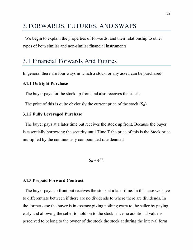
3. FORWARDS, FUTURES, AND SWAPS

We begin to explain the properties of forwards, and their relationship to other

types of both similar and non-similar financial instruments.

3.1 Financial Forwards And Futures

In general there are four ways in which a stock, or any asset, can be purchased:

3.1.1 Outright Purchase

The buyer pays for the stock up front and also receives the stock.

The price of this is quite obviously the current price of the stock (S!).

3.1.2 Fully Leveraged Purchase

The buyer pays at a later time but receives the stock up front. Because the buyer

is essentially borrowing the security until Time T the price of this is the Stock price

multiplied by the continuously compounded rate denoted

𝐒𝟎 ∗ 𝐞𝐫𝐓.

3.1.3 Prepaid Forward Contract

The buyer pays up front but receives the stock at a later time. In this case we have

to differentiate between if there are no dividends to where there are dividends. In

the former case the buyer is in essence giving nothing extra to the seller by paying

early and allowing the seller to hold on to the stock since no additional value is

perceived to belong to the owner of the stock the stock at during the interval form

13

Time 0 to Time T. Even assuming that the return on the stock will be some

calculated return, denoted (α), we then discount this return to Time 0 and are left

with the original price of the Stock, because,

𝐒𝟎 ∗ 𝐞𝛂𝐓 ∗ 𝐞!𝛂𝐓= 𝐒𝟎.

Thus the price of the Prepaid Forward will be the same as the current stock Price,

or

𝐅𝟎,𝐓𝐏 = 𝐒𝟎.

Additionally, since if the price of one was greater than the other one could easily

construct a portfolio which contains arbitrage, buy buying the one that is lower,

and selling the one that is higher.

In the scenario where there are dividends on the stock that is being purchased

under a prepaid forward contract, however, the above logic does not hold true. In

this case, the buyer should be paying less than the Stock Price. Because he is only

receiving the stock at a later date, he is not receiving the dividends that are paid

during that interim, and thus the value of the stock to the buyer is decreased by the

amount of the value of those dividends.

In the case of discrete dividends, the value of the Prepaid Forward can therefore

be written as

14

𝐅𝟎,𝐓𝐏 = 𝐒𝟎 – 𝐃𝐢𝐯 ∗ 𝐞!𝐫𝐢𝐧𝐢!𝟎 .

In the case of continuous dividends, where δ is the continuous dividend yield

from that particular index, this can be written as

𝐅𝟎,𝐓𝐏 = 𝐒𝟎*𝐞!𝛅𝐓.

In both of these cases the value of the Prepaid Forward is calculated as the stock

price deducted by the amount of the dividends that the buyer of the Prepaid

Forward is forgoing by receiving the stock at time T.

3.1.4 Forward Contract

The buyer pays at a later time and the buyer receives the stick at al a later time.

Essentially, this is the exact same thing as the Prepaid Forward Contract except

that the payment is made at Time T, and therefore we can calculate the price of a

Forward by simply calculating the Future value of the Prepaid Forward Contract.

Thus,

𝐅𝟎,𝐓 = 𝐅𝟎,𝐓𝐏 𝐞𝐫𝐓

and since

𝐅𝟎,𝐓𝐏 = 𝐒𝟎*𝐞!𝛅𝐓

15

we can rewrite

𝐅𝟎.𝐓 = 𝐅𝟎,𝐓𝐏 𝐞𝐫𝐓

as

𝐅𝟎,𝐓 =𝐒𝟎*𝐞!𝛅𝐓*𝐞𝐫𝐓

= 𝐒𝟎*𝐞(𝐫!𝛅)𝐓

Therefore there are two equivalent equations that we can use to calculate the Price

of a Forward Contract:

𝐅𝟎,𝐓 = 𝐅𝟎,𝐓𝐏 𝐞𝐫𝐓 = 𝐒𝟎𝐞(𝐫!𝛅)𝐓

We can therefore understand the configuration of a synthetic forward. In order to

duplicate the structure of the long forward which has a payoff of

𝐒𝐓 - 𝐅𝟎,𝐓

16

we create the same payoff by borrowing

𝐒𝟎𝐞!𝛅𝐓

and using the borrowed funds to buy an index in the stock. Then at time T the

borrower has to pay back

𝐒𝟎𝐞(𝐫!𝛅)𝐓

but keeps the amount of the stock, ( S!), so that his net total will be

𝐒𝐓 − 𝐒𝟎𝐞(𝐫!𝛅)𝐓

= 𝐒𝐓 - 𝐅𝟎,𝐓

This formula provides the ability and understanding that one can do what is

known as asset allocation which means that if one believes that the index that is

held may go down, rather than sell the position on the index, one can keep the

stock and short the forward. Because

17

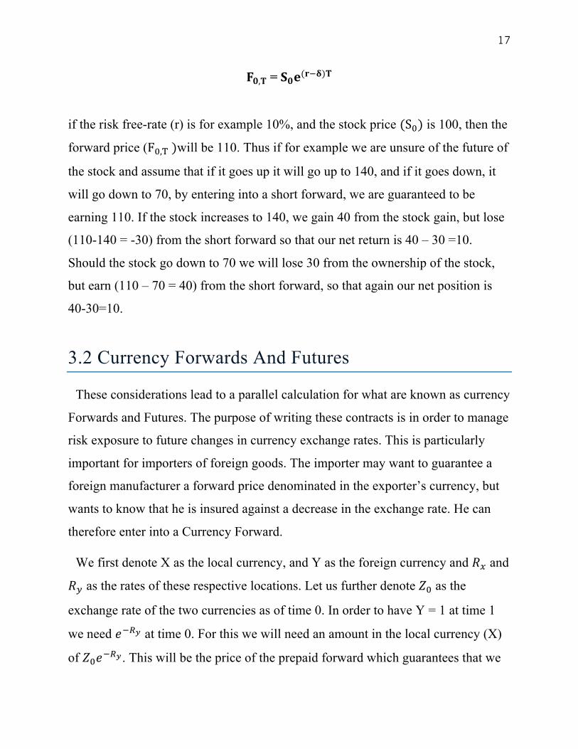
𝐅𝟎,𝐓 = 𝐒𝟎𝐞(𝐫!𝛅)𝐓

if the risk free-rate (r) is for example 10%, and the stock price (S!) is 100, then the

forward price (F!,! )will be 110. Thus if for example we are unsure of the future of

the stock and assume that if it goes up it will go up to 140, and if it goes down, it

will go down to 70, by entering into a short forward, we are guaranteed to be

earning 110. If the stock increases to 140, we gain 40 from the stock gain, but lose

(110-140 = -30) from the short forward so that our net return is 40 – 30 =10.

Should the stock go down to 70 we will lose 30 from the ownership of the stock,

but earn (110 – 70 = 40) from the short forward, so that again our net position is

40-30=10.

3.2 Currency Forwards And Futures

These considerations lead to a parallel calculation for what are known as currency

Forwards and Futures. The purpose of writing these contracts is in order to manage

risk exposure to future changes in currency exchange rates. This is particularly

important for importers of foreign goods. The importer may want to guarantee a

foreign manufacturer a forward price denominated in the exporter’s currency, but

wants to know that he is insured against a decrease in the exchange rate. He can

therefore enter into a Currency Forward.

We first denote X as the local currency, and Y as the foreign currency and 𝑅! and

𝑅! as the rates of these respective locations. Let us further denote 𝑍! as the

exchange rate of the two currencies as of time 0. In order to have Y = 1 at time 1

we need 𝑒!!! at time 0. For this we will need an amount in the local currency (X)

of 𝑍!𝑒!!! . This will be the price of the prepaid forward which guarantees that we

18

have this amount of foreign currency at time T. We can thus write the following

equation for the prepaid forward:

𝐅𝟎,𝐓𝐏 = 𝒁𝟎𝒆!𝑻𝑹𝒚

Because the importer is giving money towards this contract at time 0 he is

forfeiting otherwise possible interest gains. The formula reflects this loss just as in

the parallel stock equivalent the formula reflects an absence of the stock dividends

that the buyer of the prepaid forward is forfeiting.

We can also use this information to calculate the forward price of such a contract

by calculating the future value of the prepaid forward since as we have seen in the

case of a stock,

𝐅𝟎,𝐓 = 𝐅𝟎,𝐓𝐏 𝐞𝐫𝐓 = 𝐒𝟎𝐞(𝐫!𝛅)𝐓

Thus here as well,

𝐅𝟎.𝐓 = 𝐅𝟎,𝐓𝐏 𝐞𝐫𝐓 = 𝒁𝟎𝒆 𝑹𝒙!𝑹𝒚 𝑻

It is interesting to note that whenever

𝑹𝒙 > 𝑹𝒚

the forward currency price (F!.!) will be greater than the exchange rate (Z).

19

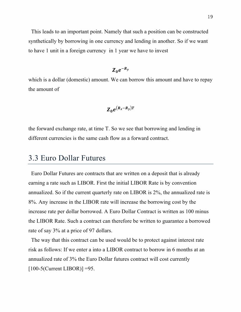
This leads to an important point. Namely that such a position can be constructed

synthetically by borrowing in one currency and lending in another. So if we want

to have 1 unit in a foreign currency in 1 year we have to invest

𝒁𝟎𝒆!𝑹𝒚

which is a dollar (domestic) amount. We can borrow this amount and have to repay

the amount of

𝒁𝟎𝒆 𝑹𝒙!𝑹𝒚 𝑻

the forward exchange rate, at time T. So we see that borrowing and lending in

different currencies is the same cash flow as a forward contract.

3.3 Euro Dollar Futures

Euro Dollar Futures are contracts that are written on a deposit that is already

earning a rate such as LIBOR. First the initial LIBOR Rate is by convention

annualized. So if the current quarterly rate on LIBOR is 2%, the annualized rate is

8%. Any increase in the LIBOR rate will increase the borrowing cost by the

increase rate per dollar borrowed. A Euro Dollar Contract is written as 100 minus

the LIBOR Rate. Such a contract can therefore be written to guarantee a borrowed

rate of say 3% at a price of 97 dollars.

The way that this contract can be used would be to protect against interest rate

risk as follows: If we enter a into a LIBOR contract to borrow in 6 months at an

annualized rate of 3% the Euro Dollar futures contract will cost currently

[100-5(Current LIBOR)] =95.

20

6 months later if the LIBOR Rate has increased to 5% our borrowing expense will

have risen [5-3] = 2. However by simultaneously having entered into a short Euro

Dollar Futures Contract which will then be at [100-5(Current LIBOR)] = 95 so that

we will now gain the difference of the Euro Dollar Futures contract as [97-95] = 2.

In a similar way, these positions can of course be reversed by going long in the

Euro Dollar Futures.

3.4 Commodity Forwards And Futures

Essentially commodity forwards and futures reflect those of financial forwards

and therefore their pricing resembles them. If the discount factor for the

commodity is 𝛽, the price of the prepaid forward will be

𝐅𝟎,𝐓𝐏 = 𝒆!𝜷𝑻 * E[S]

where E[S] is the expected spot price at time t, and therefore its forward price is

𝐅𝟎.𝐓 = 𝐅𝟎,𝐓𝐏 𝐞𝐫𝐓 = 𝐄[𝐒]𝐞!(𝜷!𝐫)𝐓

just as with financial forwards.

There are two main differences to note when calculating the forward price of a

commodity. Firstly an adjustment must be made for the storage of the commodity

(which we can denote as s). Storage is an unavoidable cost and cannot be ignored.3

3 See McDonald (pp. 202) who defines this cost as a ‘lease rate’ and explains it in terms of discounted cash flows by letting some variable be the equilibrium discount rate for an asset with the same risk as the commodity.

21

An additional adjustment must be made to the price for what is known as a

convenience yield, which is defined as a non monetary return that the holder of the

commodity gains by merely having physical possession of the commodity. This

possession gives its owner the insurance that in the event that the price of the

commodity rises he will remain unaffected, and it will not disturb his business

cycle although he may be largely reliant on the commodity. The convenience yield

(which we can denote as c) that is gained must also be calculated into the price of

the forward on the commodity so that the ending forward price for a commodity

should be

𝐅𝟎.𝐓 = 𝐒𝟎𝐞(𝐫!𝐜!𝐬)𝐓,

which denotes the total cost to the buyer of the commodity as a reflection of his

paying for the future value of the commodity, including the interest rate, and the

storage cost, less the amount of the convenience yield. This is largely applicable

when wishing to calculate an entire production for a commodity. To do so, we

simply sum the respective forward rates over each period, while compensating for

any additional cost per unit of the commodity and any other initial investments or

fixed costs. If we suppose that, for example ,at each time 𝑡!, where x goes from

1,2…n, we expect to produce 𝑛𝑡! units of the commodity, we can then calculate

the total Net Present Value for the commodity held operation as

𝒏𝒕𝒙 𝐅𝟎.𝐓𝒙 −𝑴𝒈 𝒕𝒙 𝒆!𝒓 𝟎,𝒕𝒙 𝒕𝒙 𝒏

𝒙!𝟏

–𝑪

22

where Mg is the Marginal cost per unit of the commodity that is produced, and C is

the fixed cost of the project. More complicated adjustments for specific

commodities do arise as may be necessary for commodities in the energy market

such as oil, electricity, and natural gas. Although these specific adjustments are

beyond the scope of this paper, we note this so that the reader may be aware that

each commodity may differ with respect to its particular circumstance(s).

3.5 Interest Rate Forwards And Futures

For zero-coupon bonds the price of the bond is the Present Value of the

Redemption Value, which is defined as

𝑷𝒓𝒊𝒄𝒆 = 𝑪𝒆!𝜹𝒕,

where 𝐶 is the redemption value, and 𝛿 is the continuously compounded rate.

This is particularly useful when we observe the price, and want to calculate the

corresponding yield. The yield is then (where 𝐶 is 1), just

𝜹 = 𝐥𝐧 𝟏𝑷𝒓𝒊𝒄𝒆

∗ (𝟏𝒕) .

What is relevant to our discussion is how forward and futures contracts could be

used to protect against changes in the interest rate. These contracts are known as an

FRA, or Forward Rate Agreement, and are written to give a borrower a previously

23

agreed upon rate on a loan regardless of changes in the interest rate. The agreed

upon rate is the implied forward rate. When the actual rate at the time the FRA is

settled, the parties must calculate the difference between the actual rate and the

implied forward rate and the borrower must pay the difference times the principal

amount that is borrowed, which may be positive or negative depending on whether

the interest rate is higher or lower than the implied forward rate that was agreed

upon. The overall agreement for the FRA is thus

(𝒓𝒓𝒆𝒂𝒍 𝒓𝒂𝒕𝒆 𝒐𝒇 𝒊𝒏𝒕𝒆𝒓𝒆𝒔𝒕 − 𝒓𝑭𝑹𝑨 𝒓𝒂𝒕𝒆) ∗ 𝑳

where L is the principal loan amount that is borrowed.

Note that the above is under the assumption that the FRA is settled at the time of

the loan repayment. In the event that the FRA is settled at the time of borrowing of

the funds this amount the borrower would then only be obliged to pay the Present

Value of that amount so that the overall payment for the FRA is

(𝒓𝒓𝒆𝒂𝒍 𝒓𝒂𝒕𝒆 𝒐𝒇 𝒊𝒏𝒕𝒆𝒓𝒆𝒔𝒕 − 𝒓𝑭𝑹𝑨 𝒓𝒂𝒕𝒆) ∗ 𝑳(1 + 𝒓𝒓𝒆𝒂𝒍 𝒓𝒂𝒕𝒆 𝒐𝒇 𝒊𝒏𝒕𝒆𝒓𝒆𝒔𝒕)

24

3.6 Commodity and Interest Rate Swaps

The definition of a swap is a contract that stipulates an exchange of fixed

payments, in exchange for a floating or variable set of payments, and thus can be

an additional strategy that is used to hedge against potential risk inherent in

variability. A swap is a calculated by setting the present value of the variable

payments equal to the present value of a correspondingly fixed set of payments.

The variable that will satisfy the equation of value for the fixed payment would

become the new payment that the buyer of the swap would be responsible to pay

per payment period. Since we would normally calculate the sum of all present

values of numerous forward contracts as

𝑵𝑷𝑽 =𝑭𝟎,𝟏𝟏 + 𝒊𝒕𝟏

+𝑭𝟏,𝟐𝟏 + 𝒊𝒕𝟐

+⋯𝑭𝒕(𝒏!𝟏),𝒕𝒏𝟏 + 𝒊𝒕𝒏

to calculate the swap rate we would similarly calculate a rate which satisfies the

value of x for

𝑵𝑷𝑽 =𝒙

𝟏 + 𝒊𝒕𝟏+

𝒙𝟏 + 𝒊𝒕𝟐

+⋯ .𝒙

𝟏 + 𝒊𝒕𝒏

In contrast to a forward contract, which calls for different payments at time 𝑇! and

time 𝑇!…, the payments of a swap are fixed and in fact identical.

25

Ultimately,

𝑵𝑷𝑽 =𝑭𝟎,𝟏𝟏 + 𝒊𝒕𝟏

+𝑭𝟏,𝟐𝟏 + 𝒊𝒕𝟐

+⋯𝑭𝒕(𝒏!𝟏),𝒕𝒏𝟏 + 𝒊𝒕𝒏

=𝒙

𝟏 + 𝒊𝒕𝟏+

𝒙𝟏 + 𝒊𝒕𝟐

+⋯ .𝒙

𝟏 + 𝒊𝒕𝒏

Swaps can be entered into for commodities and also for interest rate arrangements

in which one party wishes to lock in a particular rate. These will create a fixed rate

for debt instead of an otherwise potentially volatile floating rate debt.

In order to present value the forward rates, these forward rates themselves must

first be calculated. Because these forward rates are an unknown at time 0 we must

calculate them by using the current spot rate to determine what the implied forward

rate for a particular year is. Since in general,

(𝟏 + 𝑺𝟏)(𝟏 + 𝑭𝟎,𝟏) = (𝟏 + 𝑺𝟐)𝟐

the implied forward rate for year 1 can be calculated as

(𝟏 + 𝑭𝟎,𝟏) = (𝟏 + 𝑺𝟐)𝟐

(𝟏 + 𝑺𝟏)

26

This can be repeated to solve for the implied forward rate of any future particular

year by calculating that forward rate as

(𝟏 + 𝑭𝒏!𝟐,𝒏!𝟏) = (𝟏 + 𝑺𝟐)𝒏

(𝟏 + 𝑺𝟏)𝒏!𝟏

Subsequently, these implied forward rates, are discounted by present valuing them

all to time 0, by their respective present value interest rates4.

A significant and noteworthy feature of an interest rate swap is that its cash flows

are in fact identical to buying a bond where there is a fixed stream of payments,

and a redemption payment is made at the time that the bond is redeemed. This is

because the party entering the interest rate swap, by definition, has an outstanding

loan and is now due to make a fixed stream of payments to pay back the loan, in

addition to repayment of the principal at the time that the loan is due. All the future

identical cash flows of a bond are valued by taking the present value of each one at

its respective time of payout and discounting it back to time 0 at its particular rate

of interest. The interest rate swap thus has the same dimensions as that of a bond

whose present value is calculated as

𝑷 = 𝑭𝒓𝒂𝒏 + 𝑪𝒗𝒏

4 Also see Flavell (pp.140) for a discussion on Longevity swaps which at the time written had been under

discussion for some 5 years. The two sides of such a structure would typically be: . . pay an income

stream based upon current longevity expectations; receive an income stream, usually based upon changes

in one of the OTC indices.

27

In both of these cases a stream of identical cash flows are discounted at some rate

to time 0, in order to appropriately calculate the total Net Present Value.5

This concept is also particularly relevant to the actual calculation of spot rates from

zero coupon bond rates or vice-versa, since in general,

[𝒁𝒆𝒓𝒐 𝑪𝒐𝒖𝒑𝒐𝒏 𝑩𝒐𝒏𝒅 𝑷𝒓𝒊𝒄𝒆]𝒏 =𝟏

(𝟏 + 𝑺𝒏)𝒏

5 Technically we have to differentiate between a par swap and a forward start swap. Hunt (pp. 231),

discusses the distinction between them as follows: ”Swaps are usually entered at zero initial cost to both

counterparties. A swap with this property is called a par swap, and the value of the fixed rate K for which

the swap has zero value is called the par swap rate. In the case when the swap start date is spot (i.e. the

swap starts immediately), this is often abbreviated to just the swap rate, and it is these par swap rates that

are quoted on trading screens in the financial markets. A swap for which the start date is not spot is,

naturally enough, referred to as a forward start swap, and the corresponding par swap rate is the forward

swap rate. Forward start swaps are less common than spot start swaps and forward swap rates are not

quoted as standard on market screens.”

28

4. OPTION THEORIES AND PRICING MODELS

We now begin to explain and show some of the underlying theories, structures, and pricing models, within the derivative markets.

4.1 Parity

The definition of Put-Call Parity is

𝑪 − 𝑷 = (𝐅𝟎.𝐓 −𝑲)𝒆!𝒓𝑻

This formula is best understood in the context of a synthetic forward constructed

through the purchase of a call and writing of a put. For any synthetic forward that

is created at a price that is lower than the forward price there is an intrinsic gain of

not having to pay the forward price and instead buying the asset, albeit

synthetically, at a lower price. There must therefore be a corresponding

requirement that the difference between the call and put in this transaction be

exactly equal to the present value of the difference between the forward rate and

the strike price. This philosophy, which is predicated on a no-arbitrage tolerance, is

the basis for the Put-Call Parity formula. We can compare the payoff diagrams of a

long forward and a long asset as follows:

29

We notice that the payoff of the long stock is higher than the payoff of the long

forward for all S(T). To create a synthetic long forward that has the same payoff as

the true long forward, we need to bring the payoff of the long stock down which

can be done by selling a bond, as illustrated in the following graph.

-4

-3

-2

-1

0

1

2

3

4

0 1 2 3 4 5 6 7

Long Forward Payoff

Long Forward

0

1

2

3

4

5

6

7

0 1 2 3 4 5 6 7

Long Stock Payoff

Long Stock

30

Obviously, Put-Call Parity can also be rewritten as

𝑪 − 𝑷 = 𝐅𝟎,𝐓𝐏 −𝑲𝒆!𝒓𝑻

since

𝐅𝟎,𝐓𝐏 = 𝐅𝟎.𝐓 𝒆!𝒓𝑻

because

𝐅𝟎.𝐓= 𝐅𝟎,𝐓𝐏 𝐞𝐫𝐓.

0, -3

3, 0

6, 3

0, 0

3, 3

6, 6

0, -3 3, -3 6, -3

-4

-3

-2

-1

0

1

2

3

4

5

6

7

0 2 4 6 8

Put-Call Parity

Long Stock

Combined

Short Bond

31

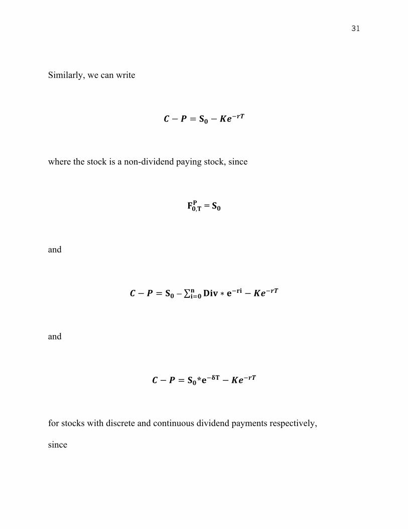
Similarly, we can write

𝑪 − 𝑷 = 𝐒𝟎 −𝑲𝒆!𝒓𝑻

where the stock is a non-dividend paying stock, since

𝐅𝟎,𝐓𝐏 = 𝐒𝟎

and

𝑪 − 𝑷 = 𝐒𝟎 – 𝐃𝐢𝐯 ∗ 𝐞!𝐫𝐢𝐧𝐢!𝟎 −𝑲𝒆!𝒓𝑻

and

𝑪 − 𝑷 = 𝐒𝟎*𝐞!𝛅𝐓 −𝑲𝒆!𝒓𝑻

for stocks with discrete and continuous dividend payments respectively,

since

32

𝐅𝟎,𝐓𝐏 = 𝐒𝟎 – 𝐃𝐢𝐯 ∗ 𝐞!𝐫𝐢𝐧𝐢!𝟎

and

𝐅𝟎,𝐓𝐏 = 𝐒𝟎*𝐞!𝛅𝐓.

The formula for Put-Call Parity also proves that a call is identical to a long position

in an asset, with a purchased put as insurance for the position when the price goes

down since

𝑪 = 𝐒𝟎 −𝑲𝒆!𝒓𝑻 + 𝑷

and that a put is identical to a short position in an asset with a purchased call as

insurance for the position when the price rises since

𝑷 = 𝐂 − (𝐒𝟎 −𝑲𝒆!𝒓𝑻)

Put-Call Parity also allows us to create a synthetic stock by replicating the stock

and thus mimicking its exact cash flows, and performance, since

𝑪 − 𝑷 = 𝐒𝟎 – 𝐃𝐢𝐯 ∗ 𝐞!𝐫𝐢𝐧𝐢!𝟎 −𝑲𝒆!𝒓𝑻

33

therefore,

𝐒𝟎 = 𝑪 − 𝑷 + 𝐃𝐢𝐯 ∗ 𝐞!𝐫𝐢𝐧𝐢!𝟎 +𝑲𝒆!𝒓𝑻

This means we can exactly replicate the stock by buying the call, selling the put,

and lending the present value of both the future dividends and the strike price.

4.2 Binomial Option Pricing

The binomial option model is a calculated approach towards pricing an option.

This model assumes a particular assumption of how the stock prices [namely 𝑆!

and 𝑆! ,where 𝑆! represents the estimated move upward in the stock price and 𝑆!

represents the estimated move downward in the stock price], will move over one or

more periods based on the historical volatility of the stock.6 What becomes

relevant to our discussion is to note that the method for computing these estimated

parameters is in fact based on the aforementioned underlying assumption that

6 This seems contrary to the approach assumed by Benth (pp.110) with regard to weather derivatives

where a classical approach is presented for pricing weather derivatives called Burn analysis, which

‘simply uses the historical distribution of the weather index/event underlying the derivative as the basis

for pricing. For example, to find a price of an option based on the HDD index in a given month, January

say, we first collect historical HDD index values from January in preceding years. Based on these records,

we generate the historical option payoffs, and simply price the option by averaging. The burn analysis

therefore corresponds to pricing by the historical expectation.'

34

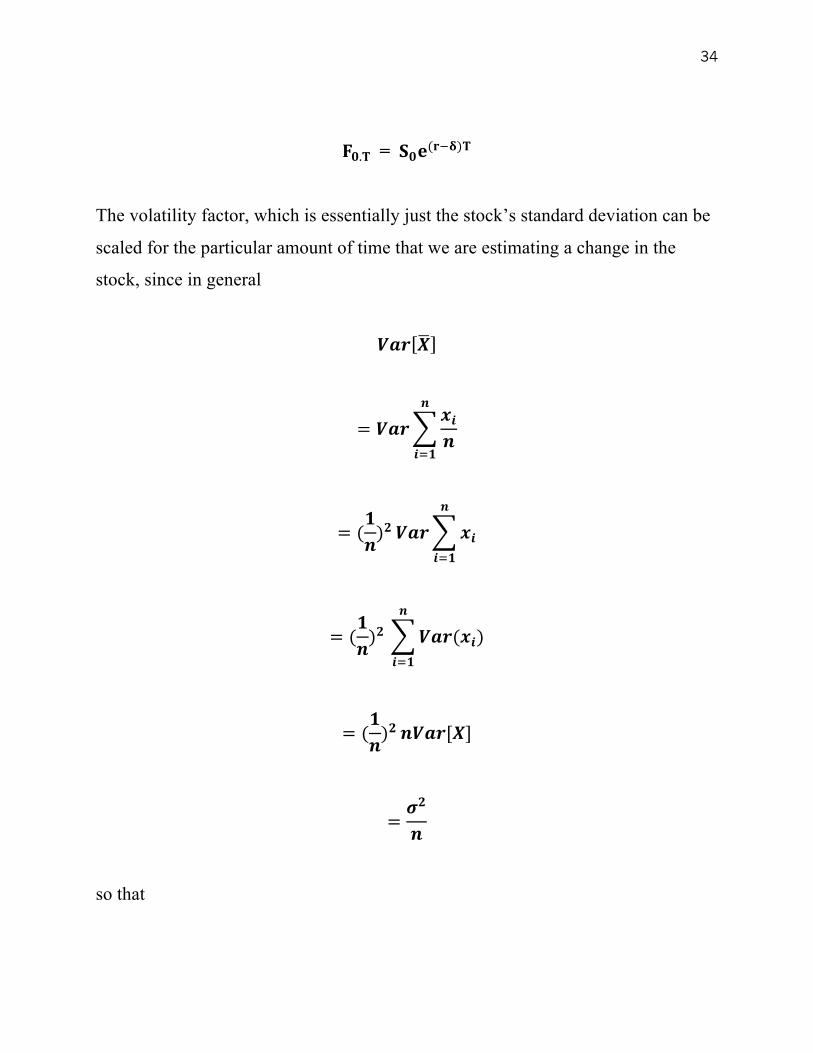
𝐅𝟎.𝐓 = 𝐒𝟎𝐞(𝐫!𝛅)𝐓

The volatility factor, which is essentially just the stock’s standard deviation can be

scaled for the particular amount of time that we are estimating a change in the

stock, since in general

𝑽𝒂𝒓 𝑿

= 𝑽𝒂𝒓𝒙𝒊𝒏

𝒏

𝒊!𝟏

= (𝟏𝒏)𝟐 𝑽𝒂𝒓 𝒙𝒊

𝒏

𝒊!𝟏

= (𝟏𝒏)𝟐 𝑽𝒂𝒓(𝒙𝒊)

𝒏

𝒊!𝟏

= (𝟏𝒏)𝟐 𝒏𝑽𝒂𝒓[𝑿]

=𝝈𝟐

𝒏

so that

35

𝝈 𝑿

= 𝝈𝟐

𝒏

= 𝝈𝒏

When analyzing historic volatility therefore we can calculate the volatility that we

expect to occur during this period as

𝝈𝑻= 𝝈(𝟏 𝑻)

This means that

𝝈(𝟏 𝑻) 𝑻 = 𝝈

It then becomes possible to calculate 𝑆! and 𝑆! as the forward price adjusted by the

volatility since in general

𝐅𝟎.𝐓 = 𝑺𝑻 = 𝐒𝟎𝐞(𝐫!𝛅)𝐓

Consequently,

𝑺𝒖 = 𝐅𝟎.𝐓𝒆(𝝈(𝟏 𝑻) 𝑻)

36

and

𝑺𝒅 = 𝐅𝟎.𝐓𝒆!(𝝈(𝟏 𝑻) 𝑻)

4.3 Lognormal Distributions for Stock Prices

In order to define and dimension the behavior of the movement of a stock we can

initially assume that returns on stocks can be of the form of a normal random

variable. Admittedly this assumption may have inefficiencies, and is in fact a

subject that can and has been disputed historically, in financial literature. In this

paper we proceed with the assumption of this parameter. The mathematical basis

and logic behind the definition of a compounded rate of return is that when as we

compound an infinite amount of times, we have

𝐥𝐢𝐦𝒏→!

𝟏 +𝒓𝒏

𝒏

= 𝒆𝒓𝑻

In the context of stock prices this means that

𝐒𝟎 ∗ 𝐞𝐫𝐓 = 𝑺𝑻

37

Consequently,

𝐥𝐧(𝑺𝑻𝐒𝟎) = 𝒓𝑻

so that once we assume the returns for a stock to be a normal random variable, the

stock price itself becomes dimensioned as that of a lognormal random variable

since,

𝑺𝑻𝐒𝟎= 𝒆𝒙

where

𝑿~𝑵(𝝁,𝝈𝟐)

Since the sum of normal random variables is also normal, by extension, the sum of

lognormal random variables is also lognormal. This means that if we assume stock

returns to be independent over time, this means that the total returns are

38

𝑬 𝑺 = 𝑬[𝑹]𝒕

𝒏

𝒕!𝟎

since in general

𝑬 𝒏𝑺 = 𝒏𝑬[𝑺]

and that the variance of the total returns is

𝑽𝒂𝒓 𝑺 = 𝑽𝒂𝒓[𝑹]𝒕

𝒏

𝒕!𝟎

since in general

𝑽𝒂𝒓 𝒏𝑺 =𝒏𝟐𝑽𝒂𝒓[𝑹]𝒕

𝒏= 𝒏𝑽𝒂𝒓[𝑹]𝒕

39

4.2 Black Scholes

The Black-Scholes formula provides an equation of value for the price of an

option. It calculates the price of the option as a consideration of six factors: Stock

Price (S), Strike Price (X), Dividend yield (𝛿), Volatility (𝜎), Interest rate (r),

Time (T), and for a (European) call is written as

𝐒𝒆!𝜹𝑻𝑵(𝒅𝟏) − 𝐊𝒆!𝒓𝑻𝑵(𝒅𝟐)

where

𝒅𝟏 =𝐥𝐧(𝑺𝑲) + (𝒓 − 𝜹 −

𝝈𝟐𝟐 )𝑻

𝝈 𝑻

and

𝒅𝟐 = 𝒅𝟏 − 𝝈 𝑻

and where 𝑁 is (calculated as) the CDF for the standard normal distribution.

Where this formula becomes essential to our previous discussion is that these

formulas can be written to calculate the price of the same option with Prepaid

forward prices since

𝒅𝟏 =𝐥𝐧(𝑺𝑲) + (𝒓 − 𝜹 −

𝝈𝟐𝟐 )𝑻

𝝈 𝑻

40

can also be written as

𝒅𝟏 =𝐥𝐧(𝑺𝒆

!𝜹𝑻

𝐊𝒆!𝒓𝑻) + (𝝈𝟐𝟐 )𝑻

𝝈 𝑻

which can then be written as

𝒅𝟏 =𝐥𝐧(

𝐅𝟎,𝐓𝐏 (𝑺)𝐅𝟎,𝐓𝐏 (𝑿)

) + (𝝈𝟐

𝟐 )𝑻

𝝈 𝑻

and the final Black Scholes Formula can then be written in terms of Prepaid

Forward Prices as

𝐅𝟎,𝐓𝐏 (𝑺)𝑵(𝒅𝟏) − 𝐅𝟎,𝐓𝐏 (𝑿)𝑵(𝒅𝟐)

41

5. INSURANCE AND RISK MANAGEMENT STRATEGIES

We next consider the structure of the insurance pricing models, and discuss their

applicability to the derivative markets, and various extensions of their principles to

risk management, and risk management strategies.

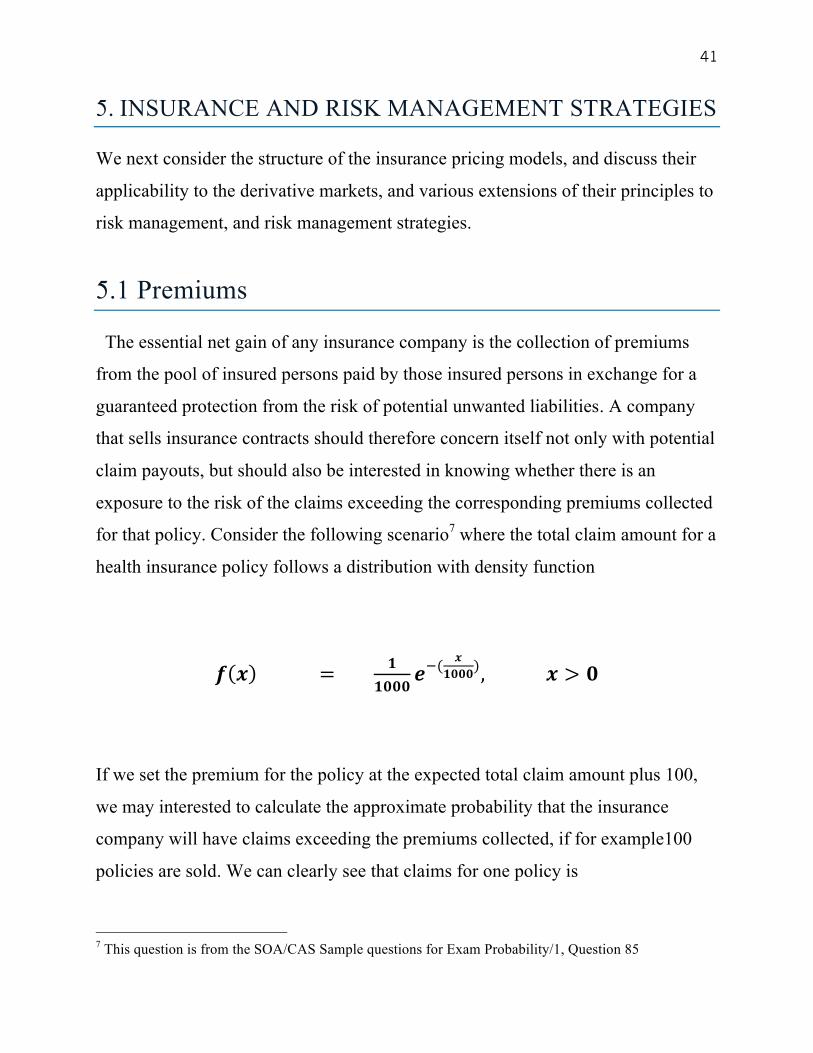
5.1 Premiums

The essential net gain of any insurance company is the collection of premiums

from the pool of insured persons paid by those insured persons in exchange for a

guaranteed protection from the risk of potential unwanted liabilities. A company

that sells insurance contracts should therefore concern itself not only with potential

claim payouts, but should also be interested in knowing whether there is an

exposure to the risk of the claims exceeding the corresponding premiums collected

for that policy. Consider the following scenario7 where the total claim amount for a

health insurance policy follows a distribution with density function

𝒇 𝒙 = 𝟏𝟏𝟎𝟎𝟎

𝒆!(𝒙

𝟏𝟎𝟎𝟎), 𝒙 > 𝟎 ��

If we set the premium for the policy at the expected total claim amount plus 100,

we may interested to calculate the approximate probability that the insurance

company will have claims exceeding the premiums collected, if for example100

policies are sold. We can clearly see that claims for one policy is

7 This question is from the SOA/CAS Sample questions for Exam Probability/1, Question 85

42

Exp. ~ 1000, 1000! , and thus the premium is 1100, the total for all 100 claims is

Exp. ~ 100,000, 10,000! , and the total for all premiums is 110,000. If we

standardize the distribution using the standard normal by subtracting 𝜇 and then

dividing by 𝜎 we get

𝒁 > [(𝒙!𝝁𝝈

) = (𝟏𝟏𝟎,𝟎𝟎𝟎!𝟏𝟎𝟎,𝟎𝟎𝟎𝟏𝟎,𝟎𝟎𝟎

) = 1] = .1587

It is therefore evident by extension, that in order to be able to calculate and manage

the risk inherent in the purchase and sale of options and hedge a position in the

option market, there must be a well-defined distribution model in order to ensure

that the premiums received for the options will produce a positive profit. The

structure of the pricing of premiums in the option market therefore, can be seen as

identical to that of the insurance pricing of premiums.

5.2 Deductibles

A key feature of insurance contracts, is a stipulation of a deductible where the

insurer only makes payment above a particular amount of loss. There can also exist

an upper deductible, where the insurer need not make payment beyond a particular

loss amount. Mathematically, where 𝑦 is the payment, 𝑥 the loss amount, 𝑑 the

deductible, and 𝑢 the upper deductible, these can be written as

𝒇 𝒚 = 𝟎 , 𝒙 < 𝒅𝒙 − 𝒅, 𝒙 > 𝒅

43

and

𝒇 𝒚 = 𝒙 , 𝒙 < 𝒖𝒖 , 𝒙 > 𝒖

respectively.

There can also exist a contract where both of these conditions apply so that the

payment is distributed as

𝒇 𝒚 = 𝟎 , 𝒙 < 𝒅

𝒙 − 𝒅 , 𝒅 < 𝒙 < 𝒖 𝒖 , 𝒖 < 𝒙

This scheme of payment is an essential difference between the insurance market,

and the option market. Seemingly, there can exist the possibility in the financial

markets for an investor to want to purchase insurance for when a particular asset

decreases in value, but is also willing to bear losses that are below a certain fixed

level. This is essentially a deductible in the insurance market, and can in fact exist

in the options market as well8. Suppose for example that one is only concerned

with large losses for a particular asset, either because only large losses are

expected, or because of the lack of funds that would be required to compensate

such a loss. Because small losses are not a concern, there is no logical reason to

pay a premium for small losses and one would rather agree to pay the ‘deductible’,

8 See for example Bellalah Chapter 21, for a discussion on many different types of Exotic Options,

including Pay-later, Chooser, Compound, Forward Start, Gap, Barrier, and Binary Options, and also

options on Maximum, or Minimum of two assets. Under a gap option (pp.906) the structure of the option

would in fact seem to be conceptually reminiscent to a deductible for an insurer.

44

in the event of peril. By extended reasoning, similar discussion is applicable for

that of upper deductibles and from the perspective of the writer of such options.

Another scenario of where the concept of a deductible could be applicable in the

option market is where there is an estimated probability that an asset will go down

to 0, but there is a model for any losses above 0. This is best illustrated by

example9: Suppose that an auto insurance company insures an automobile worth

15,000 for one year under a policy with a 1,000 deductible. During the policy year

there is a 0.04 chance of partial damage to the car and a 0.02 chance of a total loss

of the car. If there is partial damage to the car, the amount of damage (in

thousands) follows a distribution with density function

𝒇 𝒙 = .𝟓𝟎𝟎𝟑𝒆!𝒙𝟐 , 𝟎 < 𝒙 < 𝟏𝟓𝟎, 𝒐𝒕𝒉𝒆𝒓𝒘𝒊𝒔𝒆

�� In order to calculate the expected claim payment we need to consider all the

possible circumstances of peril, and in the case of partial losses perform integration

by parts so that we have:

𝟎.𝟗𝟒 𝟎 + 𝟎.𝟎𝟐 𝟏𝟓 − 𝟏 + 𝟎.𝟎𝟒 𝐱 − 𝟏 𝟎.𝟓𝟎𝟎𝟑𝐞!𝐱𝟐 𝐝𝐱

𝟏𝟓

𝟏

9 This question is from the SOA/CAS Sample questions for Exam Probability/1, Question 54

45

= 𝟎 + 𝟎.𝟐𝟖 + 𝟎.𝟎𝟐𝟎𝟎𝟏𝟐 𝐱 − 𝟏 𝟎.𝟓𝟎𝟎𝟑𝐞!𝐱𝟐 𝐝𝐱

𝟏𝟓

𝟏

= 𝟎 + 𝟎.𝟐𝟖 + 𝟎.𝟎𝟐𝟎𝟎𝟏𝟐[−𝟐𝒆!𝟕.𝟓 𝟏𝟒 − 𝟒𝒆!𝟕.𝟓 + 𝟒𝒆!𝟎.𝟓]

= 𝟎 + 𝟎.𝟐𝟖 + 𝟎(.𝟎𝟐𝟎𝟎𝟏𝟐)(𝟐.𝟒𝟎𝟖)

= 𝟎.𝟑𝟐𝟖 (in thousands)

In the options market, the analysis of an asset based on a model that has a

piecewise function such as this one would be extremely beneficial to an investor

who estimates these probabilities of risk exposure. An optimal strategy that would

follow from this expected claim amount would be to allocate the written put or

selling of the insurance contract, in a way that can resemble and therefore replicate

the possible claim amount. This will not only ensure the insurers capacity for

liability payments in the event of peril but also lower the cost for the investor, and

ultimately provide a customized insurance strategy for the investor just as it would

for any insurance company. By further creativity and modeling, these and other

similar strategies can thus become an integrated and innovative approach to

enhancing and developing the derivative markets.

46

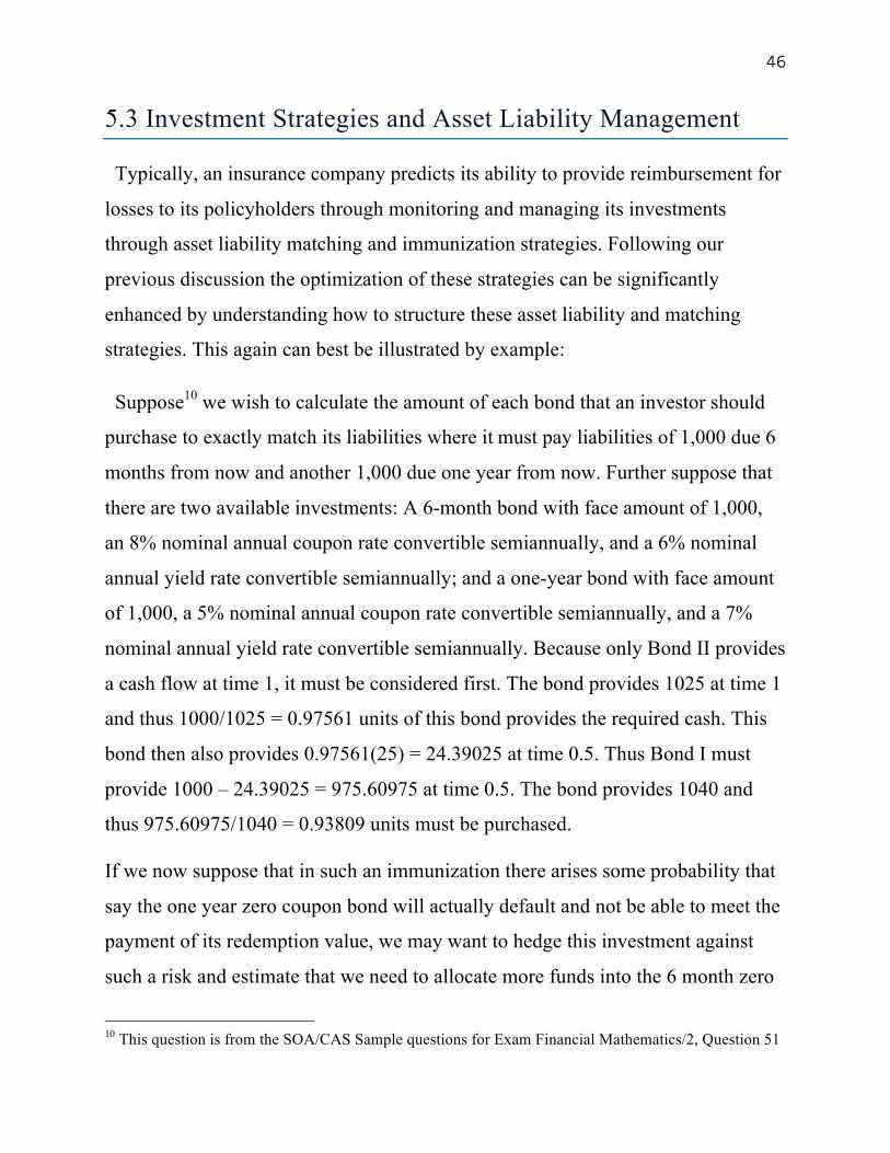
5.3 Investment Strategies and Asset Liability Management

Typically, an insurance company predicts its ability to provide reimbursement for

losses to its policyholders through monitoring and managing its investments

through asset liability matching and immunization strategies. Following our

previous discussion the optimization of these strategies can be significantly

enhanced by understanding how to structure these asset liability and matching

strategies. This again can best be illustrated by example:

Suppose10 we wish to calculate the amount of each bond that an investor should

purchase to exactly match its liabilities where it must pay liabilities of 1,000 due 6

months from now and another 1,000 due one year from now. Further suppose that

there are two available investments: A 6-month bond with face amount of 1,000,

an 8% nominal annual coupon rate convertible semiannually, and a 6% nominal

annual yield rate convertible semiannually; and a one-year bond with face amount

of 1,000, a 5% nominal annual coupon rate convertible semiannually, and a 7%

nominal annual yield rate convertible semiannually. Because only Bond II provides

a cash flow at time 1, it must be considered first. The bond provides 1025 at time 1

and thus 1000/1025 = 0.97561 units of this bond provides the required cash. This

bond then also provides 0.97561(25) = 24.39025 at time 0.5. Thus Bond I must

provide 1000 – 24.39025 = 975.60975 at time 0.5. The bond provides 1040 and

thus 975.60975/1040 = 0.93809 units must be purchased.

If we now suppose that in such an immunization there arises some probability that

say the one year zero coupon bond will actually default and not be able to meet the

payment of its redemption value, we may want to hedge this investment against

such a risk and estimate that we need to allocate more funds into the 6 month zero

10 This question is from the SOA/CAS Sample questions for Exam Financial Mathematics/2, Question 51

47

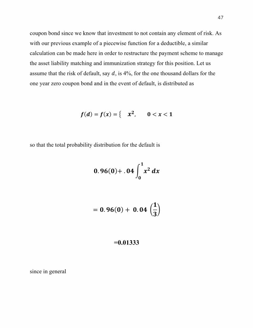
coupon bond since we know that investment to not contain any element of risk. As

with our previous example of a piecewise function for a deductible, a similar

calculation can be made here in order to restructure the payment scheme to manage

the asset liability matching and immunization strategy for this position. Let us

assume that the risk of default, say 𝑑, is 4%, for the one thousand dollars for the

one year zero coupon bond and in the event of default, is distributed as

𝒇 𝒅 = 𝒇 𝒙 = 𝒙𝟐, 𝟎 < 𝒙 < 𝟏

so that the total probability distribution for the default is

𝟎.𝟗𝟔 𝟎 + .𝟎𝟒 𝒙𝟐 𝒅𝒙𝟏

𝟎

= 𝟎.𝟗𝟔 𝟎 + 𝟎.𝟎𝟒 𝟏𝟑

=0.01333

since in general

48

𝑷 𝑨 = 𝑷 𝑨 𝑩 𝑷 𝑩 + 𝑷 𝑨 𝑩′ 𝑷 𝑩′

and

𝑬 𝑿 = 𝒇(𝒙)𝒅𝒙!

!!

We can therefore conclude that in order to ensure the 1025 at time one, a different

amount of the bond must be purchased since it really only has an expected value of

1 - 0.01333 = 0.98666(1025) = 1,011.333

1000/1011.33 = 0.98879 units of this bond provides the required cash. This bond

then also provides 0.98879(25) = 24.71975 at time 0.5. Thus Bond I must provide

1000 – 24.71975 = 975.28025 at time 0.5. The bond provides 1040 and thus

975.28025/1040 = 0.937769 units must be purchased.

We summarize these differences in Table A-1 below:

Before adjusting for

risk exposure

After adjusting for

risk exposure

Amount of units

invested of Bond I 0.93809 0.937769

Amount of units

invested of Bond II 0.97651 0.98879

TABLE A-1. EXAMPLE OF INVESTMENT AND ASSET LIABILITY MATCHING

RISK MANAGEMENT

49

5.4 Risk Assumptions and Classes

We conclude our paper with an important observation about general risk

assumptions and assessments that must be considered by insurers and investors,

since these are an important aspect of actuarial principle. There is an inherent goal

among insurers that on average a policyholder’s premium must be proportional to

his or her particular loss potential, as measured by specific rating variables. A plan

can then categorize potential customers based on the values of the rating variables.

In a competitive insurance market, insurers may constantly be refining their class

plans. Since as we have previously noted, the sale of insurance, is analogous to the

writing of a put option in the options market, we can reason that an investor who

wishes to measure his potential exposure to risk from his writing a put contract on

a selection of any given assets must often be able to class the risk of those assets.

Similarly, an investor who simply wants to short a portfolio of some group of

assets, must also be able to class the risk of those assets. In an optimal risk

management setting, it is important to identify the key risk indicators to use as

rating variables, and the discounts or surcharges based on their value.

These classes and risk variables can prove to be the greatest foundation for any

risk management procedure. For example, consider the following data of losses for

a group of 1000 policyholders, where we class according to age and health:

Age Health

Poor Average

0-50 35% 10%

50-100 30% 25%

TABLE A-2. EXAMPLE OF DATA LOSSES BY AGE AND HEALTH CLASS

50

If we class each group separately, we may be able to model the loss distribution in

a way such as the following:

Age Health

Poor Average

0-50 𝟏𝟏𝟎

𝒆!𝒙𝟏𝟎

𝟏𝟏𝟓

𝒆!𝒙𝟏𝟓

50-100 𝟏𝟐𝟎

𝒆!𝒙𝟐𝟎

𝟏𝟑𝟎

𝒆!𝒙𝟑𝟎

TABLE A-3. EXAMPLE OF LOSS DISTRIBUTION BY AGE AND HEALTH CLASS

Under this assumption the total expected payout would be:

𝟎.𝟑𝟓𝟏𝟏𝟎

𝒆!𝒙𝟏𝟎

𝟓𝟎

𝟎𝒅𝒙 + 𝟎.𝟏𝟎

𝟏𝟏𝟓

𝒆!𝒙𝟏𝟓 𝒅𝒙 +

𝟓𝟎

𝟎𝟎.𝟑𝟎

𝟏𝟐𝟎

𝒆!𝒙𝟐𝟎

𝟏𝟎𝟎

𝟓𝟎𝒅𝒙

+𝟎.𝟐𝟓𝟏𝟑𝟎

𝒆!𝒙𝟑𝟎

𝟏𝟎𝟎

𝟓𝟎𝒅𝒙

= 𝟎.𝟑𝟒𝟕𝟔 + 𝟎.𝟎𝟗𝟑𝟑 + 𝟎.𝟎𝟐𝟐𝟔 + 𝟎.𝟎𝟑𝟖𝟑 = 𝟎.𝟓𝟎𝟏𝟖

We may want to consider a particular age of having some tendency towards lower

losses, for example 0-50, since overall they only account for 45% of all losses.

Because we would be grouping the class in a different way our loss distribution

model would change as would our expected payout. Similarly, we may want to say

51

that a particular level of health is more prone towards a lower level of losses, for

example that of the average health class who account for only 35% of all losses.

This too would require us to choose a new frequency of loss distribution for each

health class. A third consideration may be to want to say that a tendency towards

lower losses due to health factors, may itself be because those health factors

themselves are a result of age. This would again require us to mitigate the original

loss assumption models and would ultimately change our expected payout. We

thus that in order to be able to understand and properly modify model loss

distributions, and thereby assess and manage risk we must also be aware of the

foundational and fundamental importance of risk assumptions and classes.

52

6. CONCLUSION

This paper has been written as a foundational tool to understand the broader

structure of the derivative markets, and in which ways they can be seen as a

parallel to the insurance industry. We have developed and explained the relevance of numerous financial

instruments, in the context of risk management, as well as provided clarification of

actuarial methods and principles.

We have showed significant attention towards understanding the relevancy of

insurance models, including payment and loss distributions, and how these affect

asset liability management and risk classes and assumptions.

We have displayed through mathematical and logical comparison, the effects that

insurance models can have on an asset, and showed that a further understanding of

these principles can platform a more adequate and strategic position held by an

investor in the derivative markets.

53

7. BIBLIOGRAPHY

[1]. Bellalah, Mondher. Derivatives, Risk Management and Value Basic

Theory, Applications and Extensions - From Theory to the Practice of

Derivatives. Singapore, US: WSPC, 2009. ProQuest ebrary. Web. 29

December 2016.

[2]. Benth, Fred Espen, And Benth, Jurate Aealtyte. Advanced Series On

Statistical Science And Applied Probability : Modeling And Pricing In

Financial Markets For Weather Derivatives. Singapore, Us: Wspc, 2012.

Proquest Ebrary. Web. 18 December 2016.

[3]. Benrud, Erik, Filbeck, Greg, And Upton, R. Travis. Derivatives And Risk

Management. Chicago, US: Dearbon Trade, A Kaplan Professional

Company, 2005. Proquest Ebrary. Web. 29 December 2016.

[4]. Flavell, Richard R.. The Wiley Finance Ser. : Swaps and Other

Derivatives (2). Hoboken, GB: John Wiley & Sons, Incorporated, 2011.

ProQuest ebrary. Web. 29 December 2016.

[5]. Hunt, P. J., and Kennedy, Joanne. Financial Derivatives in Theory and

Practice. Hoboken, NJ, USA: John Wiley & Sons, 2004. ProQuest ebrary.

Web. 29 December 2016.

[6]. McDonald, Robert L. Derivatives Markets. Boston: Pearson, 2013. Print.

[7]. N.p., n.d. Web. <https://www.soa.org/Files/Edu/edu-exam-p-sample-

quest.pdf>.

[8]. N.p., n.d. Web. <https://www.soa.org/Files/Edu/2015/edu-2015-exam-fm-

ques-theory.pdf>.