AD-Rl68 531 R-TREES: A M UNANIC INDEX STRUCTURE FOR SPATIAL -liSERRCNING(U) CALIFORNIA UNIV BERKELEY ELECTRONICSRESEARCH LAO A GUTTNAN ET AL. 14 OCT 83 UCB/ERL-M83/64

UNCLASSIFIED RFOSR-TR-86-9337 AFOSR-83-9254 F/O 9/2 NLIiiliiiiiiiiiIIIIIIIIIIIIIIIIIII.

.4.

IIIII-

* . . .'o

L "o" "." *,

.l..'..._..

.* : ' '' 4'"''' ." .- '' .' . ', " ' ". ' """ "°"" . "."•". '4 ,".',",".'." . ". ." ' ,..',' ' " " " " . '32,..'

o. .. ',.... ..-. ,. . .,:.. .. ,, .. ,. ...- .. .... ,. , ., .. ' ,;, .. . : .. ,,.. ,, , .,, ,, ... ..

136..

I77 RT LSICATO OF TH. PAT

( UNCLASSIFIED

REPORT DOCUMENTATION PAGEGo REPORT SECURITY CLASSIFICATION 1b. RESTRICTIVE MARKINGS

to_ UNCLASSIFIED_______________________

SECURITY CLASSIFICATION4 AUTHORITY 3. DISTRIBUTION/AVAI LABILITY OF REPORT

____ ____ ____APPROVED FOR PUBLIC RELEASE;D ECLASSIFICA TIN/ONRDONG RA DUNCEU DISTRIBUTION UNLIMITED

FIPERFORM41IG ORGANIZATION REPOR T NUMBERISI 5. MONITORING ORGANIZATION REPORT NUMBER(S)

_____ ____ ____AFOSR-TR .86-0337NAME OF PERFORMING ORGANIZATION b. OFFICE SYMBOL 7a. NAME OF MONITORING ORGANIZATION

js (If applicable)Electronics Research Lab. jAFOSR/NM

6c. ADDRESS (City. State and ZIP Code) 7b. ADDRESS (City. State and ZIP Code)

College of Engineering Building 410University of California, Berkeley CABolnAFD 203

_________________________ 4720 oln FD 03do. NAME OF FUNOING/SPONSORING 8Sb. OFFICE SYMBO0L 9. PROCUREMENT INSTRUMENT IDENTIFICATION NUMBER

ORGANIZATION (if applicable)

AFOSRJ NMAFOSR-83-0254

Sc. ADDRESS (City. State and ZIP Code) 10. SOURCE OF FUNDING NOS.

Building 410 PROGRAM PROJECT TASK WORK UNIT

Boiling AFB, DC 20332-6448 ELEMENT NO. NO. NO. NO.

______________________ 161102F ,~~C/ A11. TITLE finclude Security Classification)

R-TREES: A DYNAMIC INDEX STRUCTURE-FOR SPATI L SEARCHING12. PERSONAL AUTHOR(SI

Antonin Guttman ,Michael Stonebraker13a. TYPE OF REPORT 13b. TIME COVERED 14 AEO EPORT (Yr.. Mo.. Day) 15. AGE COUNT

Interim FOTO14 Oct 83 30* 16. SUPPLEMENTARY NOTATION

17. COSATI CODES 18. SUBJECT TERMS (Continue on revere iftneceary and identify by block number)

* FIELD GROUP SUB. GR.

19. ABSTRACT (Continue on reverse 'if necessary and identify by block number)

seec/4~~c ELECTE

JUNO 9 0

* DI1I~FILE GOD.* 20. DISTRIBUTION/AVAILABILITY OF ABSTRACT 21. ABSTRACT SECURITY CLASSIFICATION

UNCLASSIFIED/UNLIMITED C2SAME AS RPT. 3OTIC USERS 0 UNCLASSIFIED

22. NAME OF RESPONSIBLE INDIVIDUAL 22b. TELEPHONE NUMBER 22c. OFFICE SYMBOL

CAPT THOMAS(2276507N

DO FORM 1473, 83 APR EDITION OF I JAN 73 IS OBSOLETE. UNCLASSIFIEDSECURITY CLASSIFICATION OF THIS PAGE

J.***

1. Introduction

Spatial data objects often cover areas in multi-dimensional spaces and are not

well represented by point locations. For example, map objects like counties, census

tracts etc. occupy regions of non-zero size in two dimensions. A common operation

on spatial data is to search for all objects in an area. An example would be to find

all the counties that have land within 20 miles of a particular point. This kind of

spatial search occurs frequently in computer aided design (CAD) and geo-data appli-

cations. In such applications it is important to be able to retrieve objects efficiently

according to their spatial location.

An index based on objects' spatial locations is desirable, but classical one-

dimensional database indexing structures are not appropriate to multi-dimensional

spatial searching. Structures based on exact matching of values, such as hash tables,

are not useful because a range search is required. Structures using one-dimensional

ordering of key values, such as B-trees and ISAM indexes, do not work because the

search space is multi-dimensional.

" A number of structures have been proposed for handling multi-dimensional

point data, and a survey of methods can be found ia _.[5 Cell methods [4, 8, 16] are

not good for dynamic structures because the cell boundaries must be decided in

advance. Quad trees [71 and k-d trees [31 do not take paging of secondary memory

into account. K-D-B trees 1131 are designed for paged memory but are only useful

for point data. The use of index intervals has been suggested in [IS1, but this

method cannot be used in multiple dimensions. Corner stitching [121 is an example

of a structure for two-dimensional spatial searching suitable for data objects of non-

: ., ., ,. ' .-_,'. " .' 2.. ' ., "d.. .'-.. .' '. .. "...., .. ., ..',; ." . .". . . .,". , '. .'. .-. ., ." ,.r ! ., , . ./ ,.' *..'.,<. .'. .' .".* I

AFOSR.TR. 86-0337

.

R-TREES: A DY'A iC IN.EX SIRUCTURE

FUR SPATIAL SEARCHING

ft r by "Antonin Guttman and Michael Stonebraker

Menmorandum No. UCB/ERL M83/64

14 October 19 83

°. -

',r-? " :: ..

Approved for pulic release;distribution unliited.

• - -- -1--..-..

'

ELECTRONICS RESEARCI' I-?ArfkAT y ) YCollege of Engineering ,University of California, Berkeley, CA 94720

r~' Ti3/_no rug 9wiT rw!'w!w~nwFIw FwPawV'w"M0 7WKrMa -l-.

R-TREES: A DYNAMIC INDEX STRUCTURE

FOR SPATIAL SEARCHING

by

Antonin Guttman and Michael Stonebraker

This . 4 :IDis ..t r . .

CnbIrr tl n DlVISro

Memorandum No. UCB/ERL M83/64

14 October 1983

h.

ELECTRONICS RESEARCH LABORATORY

College of EngineeringUniversity of California, Berkeley

94720

->."r ".", ,."".. ; . .. .:.' ..> .: . .' . / .: : .. ; : , .. . .:- -.:...,.,-: : ..-: .- :-.' ..;- i-;:.-:-:..v :.4.::-;.-;:-. >:; -;4:.

1. Introduction

Spatial data objects often cover areas in multi-dimensional spaces and are not

well represented by point locations. For example, map objects like counties, census

tracts etc. occupy regions of non-zero size in two dimensions. A common operation

on spatial data is to search for all objects in an area. An example would be to find

all the counties that have land within 20 miles of a particular point. This kind of

spatial search occurs frequently in computer aided design (CAD) and geo-data appli-

cations. In such applications it is important to be able to retrieve objects efficiently

according to their spatial location.

An index based on objects' spatial locations is desirable, but classical one-

dimensional database indexing structures are not appropriate to multi-dimensional

spatial searching. Structures based on exact matching of values, such as hash tables,

are not useful because a range search is required. Structures using one-dimensional

ordering of key values, such as B-trees and ISAM indexes, do not work because the

search space is multi-dimensional.

A number of structures have been proposed for handling multi-dimensional

point data, and a survey of methods can be found in [5]. Cell methods [4,8, 18] are

not good for dynamic structures because the cell boundaries must be decided in

advance. Quad trees [7] and k-d trees [3] do not take paging of secondary memory &

into account. K-D-B trees [13] are designed for paged memory but are only useful .d 1

for point data. The use of index intervals has been suggested in [15], but this

method cannot be used in multiple dimensions. Corner stitching [12] is an example

jbility Codesof a structure for two-dimensional spatial searching suitable for data objects of non-• and/or

O I t Special

• ~~~ € - '','"," .". , e~ .:3,' " "2 2s, " " " "' , ". "" "" ""- - "" " " "" " - ." " """ "" "" "° "" " ", "" '""-INS.""- "" -, "-

2

zero size, but it assumes homogeneous primary memory and is not efficient for ran-

dom searches in very large collections of data. Grid files 1101 handle non-point data

by mapping each object to a point in a higher-dimensional space. In this paper we

describe an alternative structure called an R-tree which represents data objects by

intervals in several dimensions.'

Section 2 outlines the structure of an R-tree and Section 3 gives algorithms for

searching, inserting, deleting, and updating. Results of R-tree index performance

tests are presented in Section 4. Section 5 contains a summary of our conclusions.

2. R-Tree Index Structure

An R-tree is an index structure for n-dimensional spatial objects analogous to a

B-tree [2,81. It is a height-balanced tree with records in the leaf nodes each contain-

ing an n-dimensional rectangle and a pointer to a data object having the rectangle as

a bounding box. Higher level nodes contain similar entries with links to lower nodes.

Nodes correspond to disk pages if the structure is disk-resident, and the tree is

designed so that a small number of nodes will be visited during a spatial search. The

index is completely dynamic; inserts and deletes can be intermixed with searches and

* no periodic reorganization is required.

A spatial database consists of a collection of records representing spatial

objects, and each record has a unique identifier which can be used to retrieve it. We

approximate each spatial object by a bounding rectangle, i.e. a collection of intervals,

one along each dimension:

' ~~~~I ,-(ol,..,_ )

3

where n is the number of dimensions and Ii is a closed bounded interval [a,b]

describing the extent of the object along dimension i. Alternatively Ii may have one

or both endpoints equal to infinity, indicating that the object extends outward

indefinitely.

Leaf nodes in the tree contain index record entries of the form

(I, tuple-identifier)

where tuple-identifier refers to a tuple in the database and I is an n-dimensional*

rectangle containing the spatial object it represents. Non-leaf nodes contain entries

of the form

(I, child-pointer)

where child-pointer is the address of another node in the tree and I covers all rec-

tangles in the lower node's entries. In other words, I spatially contains all data

objects indexed in the subtree rooted at I's entry.

Let M be the maximum number of entries that will fit in one node and let

m < M be a parameter specifying the minimum number of entries in a node. An R--2

tree satisfies the following properties:

(1) Every leaf node contains between m and AM index records unless it is the root.

(2) For each index record (I,tuple-identifier) in a leaf node, I is the smallest rec-

tangle that spatially contains the n-dimensional data object represented by the

indicated tuple.

(3) Every non-le3f node has between m and M children unless it is the root.

(4) For each entry (1,child-pointer) in a non-leaf node, I is the smallest rectangle

that spatially contains the rectangles in the child node.

Jb

4

(5) The root node has at leas. two children unless it is a leaf.

(6) All leaves appear on the same level.

Figure 2.1a and 2.1b show an example R-tree structure and the geometric forms

it represents.

The height of an R-tree containing N index records is at most rlog. N,

because the branching factor of each node is at least m. The maximum number of

nodes is F. i + [r_ + '-+ 1. Worst-case space utilization for all nodes except

the root is -a. Nodes will tend to have more than m entries, and this will decrease

* tree height and improve space utilization. If nodes have more than 3 or 4 entries the

tree will be very wide, and almost all the space will be used for leaf nodes containing

index records. The parameter m can be varied as part of performance tuning, and

different values are tested experimentally in Section 4.

3. Searching and Updating

3.1. Searching

The search algorithm descends the tree from the root in a manner similar to a

B-tree. However when it visits a non-leaf node it may find that any number of sub-

trees from 0 to M need to be searched; hence it is not possible to guarantee good

worst-case performance. Nevertheless with most kinds of data the update algorithms

will maintain the tree in a form that allows the search algorithm to eliminate

irrelevant regions of the indexed space, and examine only data near the search area.

;,'- " , -,- - ", ,,,' . , ' ' .' ' .- '.. .. ' .' '-.' .'. '-. -.- . . .. x -. . '. . -. . . . . - .. -. '-' . .. - _ . . .

I, ,, #, , ,. .t, "- . '. . . , , . , ., . , . - , . - .. ,, - . ' ,,.. - . ' .. ,. . . - . " . - - .. , - .. - ., ' ..

Ir

8 R10 RIo RI 112 R13 R141 R15 JR16 I ]Ri? JR16 R191

I 1 114

- - --- - - - -

-- -- -- --- -- --- -- --- -- -- -(b) 13

Fiur 2.1

I7-a

6

In the following we denote the rectangle part of an index entry E by E.1, and

the tuple-identifier or child-pointer part by E.p.

Algorithm Search. Given an R-tree whose root node is T, find all index records

whose rectangles overlap a search rectangle S.

S1. [Search subtrees.]

If T is not a leaf, check each entry E to determine whether E.1 overlaps S.

For all overlapping entries, invoke Search on the tree whose root node is

pointed to by E.p.

S2. [Search leaf node.]

If T is a leaf, check all entries E to determine whether E.I overlaps S. If so, E

is a qualifying record.

3.2. Insertion

Inserting index records for new data tuples is similar to insertion in a B-tree in

that new index records are added to the leaves, nodes that overflow are split, and

splits propagate up the tree.

Algorithm Insert. Insert a new index entry E into an R-tree.

I1. [Find position for new record.]

Invoke ChooseLea" to select a leaf node L in which to place E.

12. [Add record to leaf node.]

If L has room for another entry, install E. Otherwise invoke SplitNode to

obtain L and LL containing E and all the old entries of L.

7

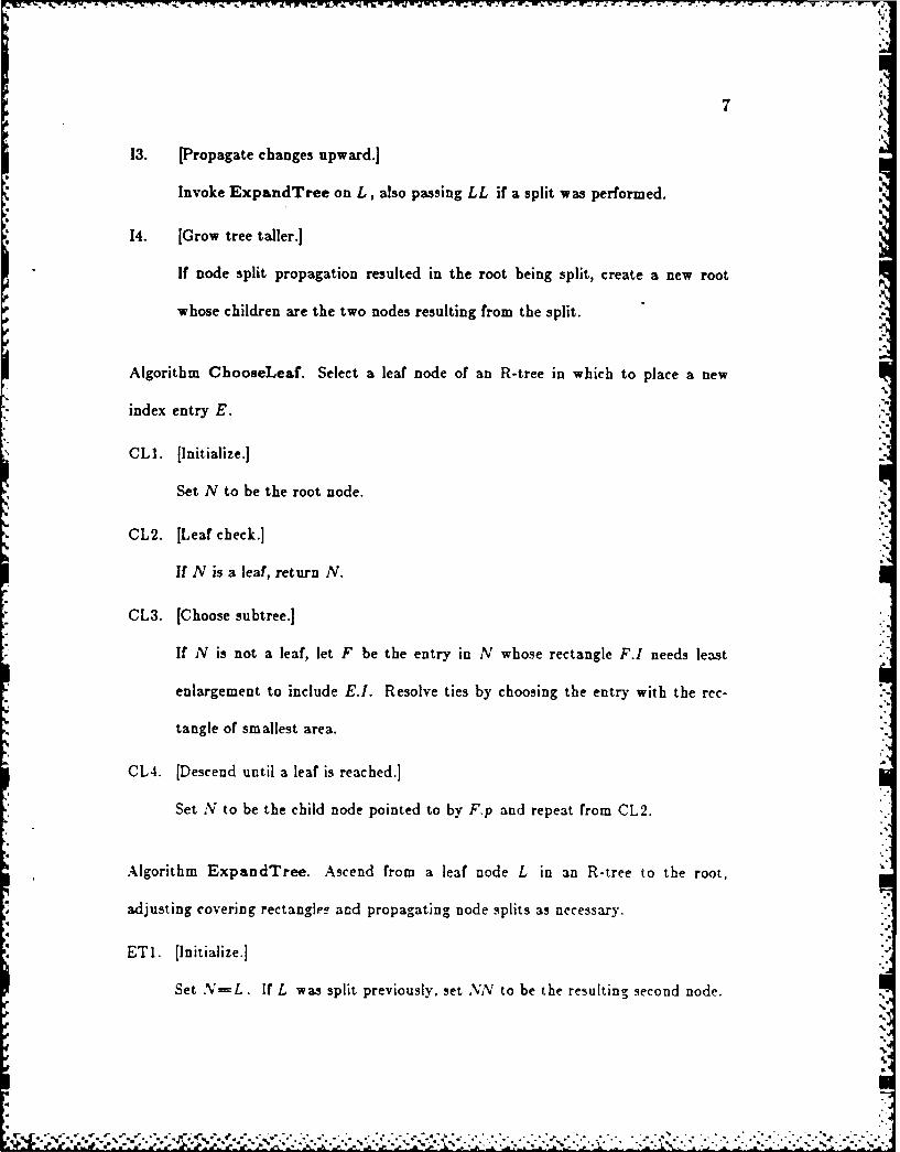
13. [Propagate changes upward.]

Invoke ExpandTree on L, also passing LL if a split was performed.

14. [Grow tree taller.]

If node split propagation resulted in the root being split, create a new root

whose children are the two nodes resulting from the split.

Algorithm ChooseLeaf. Select a leaf node of an R-tree in which to place a new

index entry E.

CLI. [Initialize.]

Set N to be the root node.

CL2. [Leaf check.]

If N is a leaf, return N.

CL3. [Choose subtree.]

If N is not a leaf, let F be the entry in N whose rectangle F.I needs least

enlargement to include E.I. Resolve ties by choosing the entry with the rec-

tangle of smallest area.

CL4. [Descend until a leaf is reached.]

Set N to be the child node pointed to by F.p and repeat from CL2.

Algorithm ExpandTree. Ascend from a leaf node L in an R-tree to the root,

adjusting covering rectangle! and propagating node splits as necessary.

ET1. [Initialize.]

Set N=L. If L was split previously, set NN to be the resulting second node.

d4

" ' . ,'.':, .. ? .y , , , ." ..- .. . , ,- ,,. ;..'. '. X y.' .

-. -, . - -. . ' .- ,,'- " _ ", . ' /." /- .' "- - " "- " ' -- - ",

ET2. [Check if done.]

If N is the root, stop.

ET3. [Adjust covering rectangle in parent entry.l

Let P be the parent node of N, and let EN be N's entry in P. Adjust E.!J

so that it tightly encloses all entry rectangles in N.

ET4. [Propagate node split upward.]

If N has a partner NN resulting from an earlier split, create a new entry ENV

with ENN.p pointing to NN and ENN.J enclosing all rectangles in AN. Add

ENN to P if there is room. Otherwise, invoke SplitNodle to produce P and

PP containing ENN,- and all P's old entries.

ET5. [Move up to next level.)

Set NP and set NN=ZPP if a split occurred. Repeat from ET2.

Algorithm SplitNode is described in Section 3.5.

3.3. Deletion

Algorithm Delete. Remove idxrecord E from an R-tree.

DI. [Find node containing record.]

Invoke FindLeaf to locate the leaf node L containing E. Stop If the record

wa, not round.

D 2. D~eetr e cord.)

Remove E frcm L.

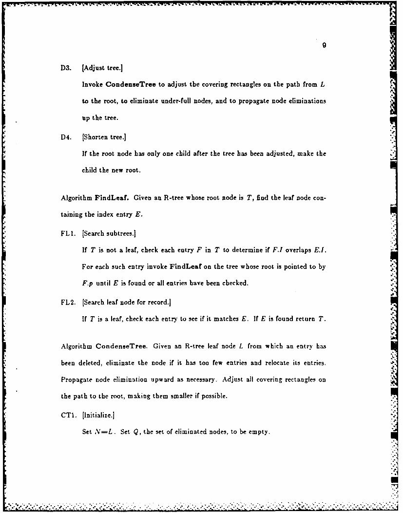
D3. [Adjust tree.]

Invoke CondenseTree to adjust the covering rectangles on the path from L

to the root, to eliminate under-full nodes, and to propagate node eliminations

up the tree.

D4. [Shorten tree.]

If the root node has only one child after the tree has been adjusted, make the

child the new root.

Algorithm FindLeaf. Given an R-tree whose root node is T, find the leaf node con-

taining the index entry E.

FLI. [Search subtrees.]

If T is not a leaf, check each entry F in T to determine if F.! overlaps E.I.

For each such entry invoke FindLeaf on the tree whose root is pointed to by

F.p until E is found or all entries have been checked.

FL2. [Search leaf node for record.]

If T is a leaf, check each entry to see if it matches E. If E is found return T.

Algorithm CondenseTree. Given an R-tree leaf node L from which an entry has

been deleted, eliminate the node if it has too few entries and relocate its entries.

Propagate node elimination upward as necessary. Adjust all covering rectangles on

the path to the root, making them smaller if possible.

CT1. [Initialize.]

Set N=L. Set Q, the set of eliminated nodes, to be empty.

7 -Z1

10

CT2. [Find parent entry unless root has been reached.]

If N is the root, go to CT6. Otherwise let P be the parent of N, and let EN

be N's entry in P.

CT3. [Eliminate under-full node.]

If N has fewer than m entries, delete EN from P and add N to set Q.

CT4. [Adjust covering rectangle.]

If N has not been eliminated, adjust EN. to tightly contain all entries in N.

CT5. [Move up one level in tree.]

Set N=P and repeat from CT2.

CT6. [Re-insert orphaned entries.]

Re-insert all entries of nodes in set Q. Entries from eliminated leaf nodes are

re-inserted in tree leaves as described in Algorithm Insert, but entries from

higher-level nodes must be placed higher in the tree. This is done so that

leaves of their dependent subtrees will be on the same level as leaves of the

main tree.

The procedure outlined above for disposing of under-full nodes differs from the

corresponding operation on a B-tree, in which two or more adjacent nodes are

merged. A B-tree-like approach is possible for R-trees, although there is no adja-

cency in the B-tree sense: an under-full node can be merged with whichever sibling

will have its area increased least, or tOe orphanued entries can be distributed among

sibling node. Either method can cause nodes to be split.

21' ~4 . . .

11

Re-insertion was chosen instead for two reasons: first, it accomplishes the same

thing and is easier to implement because the Insert routine can be used. Efficiency

should be comparable because pages needed during re-insertion usually will be the

same ones visited during the preceding search and will already be in memory. The

second reason is that re-insertion incrementally refines the spatial structure of the

tree, and prevents gradual deterioration that might occur if each entry were located

permanently under the same parent node.

3.4. Updates and Other Operations

If a data tuple is updated so that its covering rectangle is changed, its index

record must be deleted, updated, and then re-inserted, so that it will find its way to

the right place in the tree.

Other kinds of searches besides the one described above may be useful, for

example to find all data objects completely contained in a search area, or all objects

that contain a search area. These operations can be implemented by straightforward

variations on the algorithm given. A search for a specific entry whose identity is

known beforehand is required by the deletion algorithm and is implemented by Algo-

rithm FindLeaf. Variants of range deletion, in which index entries for all data

objects in a particular area are removed, are also well supported by R-trees.

3.5. Node Splitting

When an attempt is made to add an entry to a full node containing ,M entries,

the collection of M+ 1 entries must be divided between two nodes. The division

12

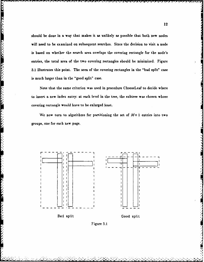
should be done in a way that makes it as unlikely as possible that both new nodes

will need to be examined on subsequent searches. Since the decision to visit a node

is based on whether the search area overlaps the covering rectangle for the node's

entries, the total area of the two covering rectangles should be minimized. Figure

3.1 illustrates this point. The area of the covering rectangles in the "bad split" case

is much larger than in the "good split" case.

Note that the same criterion was used in procedure ChooseLeaf to decide where.

to insert a new index entry: at each level in the tree, the subtree was chosen whose

covering rectangle would have to be enlarged least.

We now turn to algorithms for partitioning the set of M+ 1 entries into two

groups, one for each new page.

11

- - - -t .---- L

Bad split Good split

Figure 3.1

I I I I

I ii I I]

I° I°- • ... .. . . .. . . . ..

"I" - "I " ' ' " " " * '' -"I'' ' '' " " -" -I"" " " -" ' "." ' ' - - - .- b "- ." -;' ". ." -"- . "v .. -.-.. .- 2" "

13 K

K

3.5.1. Exhaustive Algorithm

The most straightforward way to find the minimum area node split is to gen-

erate all alternatives and choose the best. However, the number of possible parti-

tions is approximately 2 M-1 and a reasonable value of M is 50', so the number of

possible splits is very large. We implemented a modified form of the exhaustive node

split algorithm to use as a standard for comparison with other algorithms, but it was

too slow to use with large page sizes.

3.5.2. A Quadratic-Cost Algorithm

This algorithm attempts to find a small-area split, but is not guaranteed to find

one with the smallest area possible. The cost is quadratic in M and linear in the

number of dimensions. The algorithm picks two of the M+ I entries to be the first

elements of the groups which will make up the new nodes. The pair chosen is the

one that would waste the most area if both entries were put in the same group, i.e.

the area of the rectangle covering both entries, minus the areas of the rectangles inr.

the entries, would be greatest. Then the remaining entries are selected one at a time

and assigned to a group. At each step the area expansion required to add each entry

to each group is calculated, and the entry chosen is the one showing the greatest

difference between the two groups in the expansion required to include it.

Algorithm Quadratic Split. Divide a set of M+ 1 index entries into two groups.

A two dimensional rectangle can be represented by four numbers of four bytes each.If a pointer also takes four bytes, each entry requires 20 bytes. A page o 1024 bytes will holdabout 50 entries.

A.

9,'A

14

QSI. [Pick first entry for each group.]

Apply Algorithm PickSeeds to choose two entries to be the first elements of

the groups. Assign each to a group.

QS2. [Check if done.]

If all entries have been assigned, stop. If one group has so few entries that all

the rest must be assigned to it in order for it to have the minimum number

m, assign them and stop.

QS3. [Select entry to assign.)

Invoke Algorithm PickNext to choose the next entry to assign. Add it to

the group whose covering rectangle will have to be enlarged least to accommo-

date it. Resolve ties by adding the entry to the group with smaller area, then

to the one with fewer entries, then to either. Repeat from QS2.

Algorithm PickSeeds. Select two entries to be the first elements of the groups.

PSI. [Calculate inefficiency of grouping entries together.]

For each pair of entries El and E, compose a rectangle J including E1.1 and

E.!. Calculate d=- area(J) - area(El.I) - area(E,.).

PS2. [Choose the most wasteful pair.]

Choose the pair with the largest d to be put in different groups.

Algorithm PickNext. Select one remaining entry for classification in a group.

PN1. [Determine cost of putting each entry in each group.]

For each entry E not yet in a group, calculate d=- the area increase required

in the covering rectangle of Group 1 to include E.I. Calculate d.2 similarly for

Group 2.

PN2. [Find entry with greatest preference for one group.]

Choose the entry with the greatest difference between d, and d2. If more

than one has the same lowest difference pick any of them.

3.5.3. A Linear-Cost Algorithm

This algorithm is linear in M and in the number of dimensions. First it selects

seed entries for the two groups, choosing the two whose rectangles are the most

widely separated along any dimension. Then it processes the remaining entries

without ordering them in any special way, placing each in one of the groups.

Algorithm Linear Split is identical to Quadratic Split but uses a different version

of PickSeeds. PickNext simply chooses any of the remaining entries.

Algorithm LinearPickSeeds. Select two entries to be the first elements of the

groups.

LPSl. [Find extreme rectangles along all dimensions.]

Along each dimension, find the entry whose rectangle has the highest low side,

and the one with the lowest high side. Record the separation.

LPS2. [Adjust for shape of the rectangle cluster.]

Normalize the separations by dividing by the width or the entire set along the

corresponding dimension.

LPS3. [Select the most extreme pair.]

Choose the pair with the greatest normalized separation along any dimension.

16

4. Performance Tests

We implemented R-trees in C under Unix on a Vax 11/780 computer. Our

implementation has been used for a series of performance tests, whose purpose was

to verify the practicality of the structure, to choose values for M and m, and to

evaluate different node-splitting algorithms. This section presents the results.

Five page sizes were tested, corresponding to different values of M:

Bytes per Page Max Entries per Page (M)128 8258 12512 25

1024 502048 102

The minimum number of entries in a node (m) was tested for values At/2, M13, and

2. The three node split algorithms described earlier were implemented in different

versions of the program.

All our tests used two-dimensional data, although the structure and algorithms

work for any number of dimensions. During the first part of each test run the pro-

gram read geometry data from files and constructed an index tree, beginning with an

empty tree and calling Inrert with each new index record. Insert performance was

measured for the last I0% of the records, when the tree was nearly its final size.

During the second phase the program called the function Search with random

search rectangles made up using the local random number generation facility. 100

searches were performed per test run, each retrieving about 5% of the data.

Finally the program read the input files a second time and called the function

Delete to remove the index record for every tenth data item. Thus measurements

' A

17

were taken for scattered deletion of 10% of the index records.

The tests were done using Very Large Scale Integrated circuit (VLSI) layout

data from the RISC-I computer chip. [11]. The first series of tests used the circuit

cell CENTRAL, containing 1057 rectangles (Figure 4.1).Kp

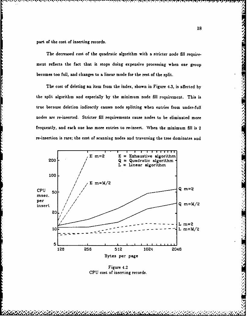
Figure 4.2 shows the cost in CPU time for inserting the last 10% of the records

as a function of page size. The exhaustive algorithm, whose cost increases exponen-

tially with page size, is seen to be very slow for larger page sizes. The linear algo-

rithm is fastest, as expected. With this algorithm CPU time hardly increased with

page size at all, which suggests that node splitting was responsible for only a small

71'

! ..

-,-

Figure 4.1

Circuit cell CENTRAL (1057 rectangles).

r;.

18

part of the cost of inserting records.

The decreased cost of the quadratic algorithm with a stricter node fill require-

ment reflects the fact that it stops doing expensive processing when one group

becomes too full, and changes to a linear mode for the rest of the split.

The cost of deleting an item from the index, shown in Figure 4.3, is affected by

the split algorithm and especially by the minimum node fill requirement. This is

true because deletion indirectly causes node splitting when entries from under-full

nodes are re-inserted. Stricter fill requirements cause nodes to be eliminated more

frequently, and each one has more entries to re-insert. When the minimum fill is 2

re-insertion is rare; the cost of scanning nodes and traversing the tree dominates and

. E m=2 E = Exhaustive algorithm200 / Q = Quadratic algorithm20L = Linear algorithm/

/100 //

mE =M/2/ / Q rn=2CPU 5 / /

perBytes er!paginsertCUcsofisrigrcrs

20./

= .. ..... L mn=2

10- L re=M/2

1 28 256 512 1024 2048

Bytes per page

Figure 4.2

CPU cost of inserting records.

19:

the split algorithm has little effect. The curves are rough because node eliminations

occur randomly and infrequently; there were too few of them in our tests to smooth

out the variations.

Figures 4.4 and 4.5 show that the search performance of the index is very insen-

sitive to the use of different node split algorithms and fill requirements. *The exhaus-

tive algorithm produces a slightly better index structure, resulting in fewer pages

touched and less CPU cost, but even the crudest algorithm, the linear one with

m=M/2, provides reasonable performance. Most combinations of algorithm and

minimum fill come within 10% of the performance achieved with node splits pro-

duced by the exhaustive algorithm.

100 , , a a , i, ., ,E = Exhaustive algorithm

E mM/2 Q = Quadratic algorithm/ L = Linear algorithm

50- L r=M/2CPU Q m=M/2msee. //

perdelete / -

20- / ..-

L m=2

10 E-"" Em=2m2

128 256 512 1024 2048

Bytes per page J.

Figure 4.3CPU cost of deleting records.

*~~~~~~~~ -5 T-7.S - -* . - .. * -

20

.6 E = Exhaustive algorithmQ = Quadratic algorithmL = Linear algorithm

Pages \ E m=2touchedper \ '

qualifying Xrecord .3E- M/ .

.2-

.1 L m=2Q m=M/2

128 256 512 1024 2045

Bytes per page

Figure 4.4Search performance: Pages touched.

E = Exhaustive algorithm500- Q = Quadratic algorithmLmM/

CPU L = Linear algorithm

usec. Q400/perLm=qualifying Q m=2record 30

300.

200 --.

E m=2 E m=M/2

125 256 512 1024 2048

Bytes per page

Figure 4.5Search performance: CPT, cost.

21

Figure 4.8 shows the storage space occupied by the index tree as a function of

algorithm, fill criterion and page size. Generally the results bear out our expectation

that stricter node fill criteria produce smaller indexes. The least dense index con-

sumes about 50% more space than the most dense, but all results for 1/2-full and

1/3-full (not shown) are within 15% of each other.

We performed a second series of tests to measure R-tree performance as a func-

tion of the amount of data in the index. The same sequence of test operations as

before was run on samples containing 1057, 2238, 3295, and 4559 rectangles. The

first sample contained layout data from the same circuit cell CENTRAL as used ear-

lier. The second sample consisted of layout from a larger circuit cell containing 2238

rectangles. The third sample was made by using both CENTRAL and the larger

E = Exhaustive algorithm50kQ = Quadratic algorithm

E m=2 L = Linear algorithm

45k "Q m=2

Bytes 40k _ --

required E m=M/235k L re=M/2

Q m=M/230k

28 256 512 1024 2048Bytes per page

Figure 4.8Space efficiency.

-...,, . ..'.u, .: -, ,,.. .. ... ,.. .. -,... ...,. .....,. . .,,.-. .....-. '.a..- ,... . .,.-.-. .-.. --. " v - a,".".... ',' .

cell, with the two cells effectively placed on top of each other. Three cells were com-

bined to make up the last sample. Because the samples were all composed in

different ways using varying data, performance results would not scale perfectly and

some unevenness was to be expected.

Two combinations of algorithm and node fill requirement were chosen for the

tests: the linear split algorithm with m=2, and the quadratic algorithm with

m=:M/3, both with a page size of 1024 bytes (M=50). Both have good search per-

formance; the linear configuration has about hair the insert cost, and the quadratic

one produces a smaller index.

Figure 4.7 shows the results of tests whose purpose was to determine how insert

and delete performance is affected by tree size. Both test configurations produced

trees with two levels for 1057 records and three levels for the other sample sizes.

The figure shows that the cost of inserts with the quadratic algorithm is nearly con-

*stant except where the tree increases in height, where the curve shows a definite

*jump because the number of levels where an expensive split can occur increases. The

linear algorithm shows no jump, indicating again that linear node splits account for

only a small part of the cost of inserts.

Deletion with the linear configuration has nearly constant cost for fixed tree

* height, and a small jump where the tree becomes taller. The tests involved too few

deletions to cause any node spiits on re-insertion with the relaxed node fill require-

ment. A few splits did occur during deletion with the quadratic configuration. but

only 1 to P3 per re~t nr'i, and the number of nodes eliminated was similarly small.

Varving between 4 and 15. Such small numbers, coupled with the high colt of node

23

Q = Quadratic algorithm, m=M/3L Linear algorithm, m=2

40

CPU msec.

per 30inserto r

Qin

delete 20 Q deleteL delete

.

1000 2000 3000 4000 5000Number of records

Figure 4.7CPU cost of inserts and deletes vs. amount of data.

eliminations, made the quadratic curve very erratic.

When allowance is made for variations due to the small sample size, the tests

show that insert and delete cost is independent of tree width but is affected by tree

height, which grows slowly with the number of data items. This performance is very

similar to that of a B-tree.

The search tests retrieved between 3% and 8% of the data on each search. Fig-

ures 4.8 and 4.9 confirm that the two configurations have nearly the same perfor-

mance. The downward trend of the curves is to be expected, because the cost of .-

processing higher tree nodes becomes less significant as the amount of data retrieved

in each search increases. The decrease would have been more uniform. but an unex-

pected variation in the 2238-item sample raised the cost at the second data point.

....................................

24

.15Q = Quadratic algorithm. m=M/3

L = Linear algorithm, m=2

Pages .1

touchedperqualifyingrecord

.05

1000 2000 3000 4000 5000

Number of records

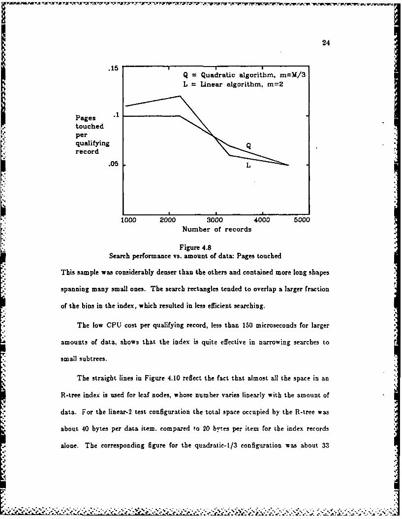
Figure 4.8Search performance vs. amount of data: Pages touched

This sample was considerably denser than the others and contained more long shapes

spanning many small ones. The search rectangles tended to overlap a larger fraction

of the bins in the index, which resulted in less efficient searching.

The low CPU cost per qualifying record, less than 150 microseconds for larger

amounts of data, shows that the index is quite effective in narrowing searches to

small subtrees.

The straight lines in Figure 4.10 reflect the fact that almost all the space in an

R-tree index is used for leaf nodes, whose number varies linearly with the amount of

data. For the linear-2 test configuration the total space occupied by the R-tree was

about 40 bytes per data item, compared to 20 bytes per item for the index records

alone. The corresponding figure for the quadratic-l/3 configuration was about 33

25 :

300

250

CPU usec.per 200-qualifyingrecord

150 -

L100.

50 Q - Quadratic algorithm, m=M/3

L = Linear algorithm, m=2

1000 2000 3000 4000 5000Number of records

Figure 4.9Search performance vs. amount of data: CPU cost

..bytes per item.

5. Conclusions

The R-tree structure has been shown to be useful for indexing spatial data Kobjects that have non-zero size. Nodes corresponding to disk pages of reasonable size

(e.g. 1024 bytes) have values of M that produce good performance. With smaller

nodes the structure should also be effective as a main-memory index; CPU perfor-

mance would be comparable but there would be no I/O cost.

The linear node-split algorithm proved to be as good as more expensive tech-

niques. It was fast, and the slightly worse quality of the splits did not affect search

performance noticeably.

7-.

,eU

26

Preliminary investigation indicates that R-trees would be easy to add to any

relational database system that supported conventional access methods, (e.g.

INGRES [9], System-R [1] ). Moreover, the new structure would work especially well

in conjunction with abstract data types and abstract indexes [14] to streamline the

handling of spatial data.

200kQ = Quadratic algorithm. m=M/3 L

," •L = Linear algorithm. m=2

Hye 150k Q~Bytes

required

100k

50k-

1000 2000 3000 4000 5000

Number of records

Figure 5.10Space required for R-tree vs. amount of data.

REFERENCESi

[1] M. Astrahan, et al., "System R: Relational Approach to Database Manage-ment," ACM Transactions on Database Systems 1(2) pp. 97-137 (June 1978).

[2] R. Bayer and E. McCreight, "Organization and Maintenance of Large OrderedIndices," Proc. 1970 ACM-SIGFIDET Workshop on Data Description andAccess, pp. 107-141 (Nov. 1970).

[3] J. L. Bentley, "Multidimensional Binary Search Trees Used for AssociativeSearching," Communications of the A CM 18(9) pp. 509-517 (September 1975).

[4] J. L. Bentley, D. F. Stanat, and E. H. Williams Jr., "The complexity of fixed-radius near neighbor searching," Inf. Proc. Lett. 8(6) pp. 209-212 (December1977).

[5] J. L. Bentley and J. H. Friedman, "Data Structures for Range Searching,"Computing Surveys 11(4) pp. 397-409 (December 1979).

([] D. Comer, "The Ubiquitous B-tree," Computing Surveys 11(2) pp. 121-138. (1979).[7] R. A. Finkel and J. L. Bentley, "Quad Trees - A Data Structure for Retrieval

on Composite Keys," Acta Informatica 4 pp. 1-9 (1974).

[8] A. Guttman and M. Stonebraker, "Using a Relational Database Management*" System for Computer Aided Design Data," IEEE Database Engineering

6(2)(June 1982).

[9] G. Held, M. Stonebraker, and E. Wong, "INGRES - A Relational Data BaseSystem," Proc. AFIPS 1975 NCC 44 pp. 409-416 (1975).

[101 K. Hinrichs and J. Nievergelt, "The Grid File: A Data Structure Designed to* Support Proximity Queries on Spatial Objects," Nr. 54, Institut fur Informatik,

Eidgenossische Technische Hochschule, Zurich (July 1983).

* [11] M.G.H. Katevenis, R.W. Sherburne, D.A. Patterson, and C.H. S4quin, "TheRISC II Micro-Architecture," Proc. VLSI 83 Conference, (August 1983).

" [12] J. K. Ousterhout, "Corner Stitching: A Data Structuring Technique for VLSILayout Tools," Computer Science Report CSD 82/114, University of California,Berkeley (1982).

[13] J. T. Robinson, "The K-D-B Tree: A Search Structure for Large Multidimen-sional Dynamic Indexes," ACM-SIGMOD Conference Proc., pp. 10-18 (April1981).

114] M. Stonebraker, B. Rubenstein, and A. Guttman, "Application of AbstractData Types and Abstract Indices to CAD Data Bases," Memorandum No.UCB/ERL M83/3. Electronics Research Laboratory, University of California,Berkeley (January 1983).

[15] K. C. Wong and M. Edelberg, "Interval Hierarchies and Their Application to

27

28

Predicate Files," A CM Transactions on Database Systems 2(3) pp. 223-232 (Sep-tember 1977).

1181 G. Yuval, "Finding Near Neighbors in k-dimensional Space," Inf. Proc. Left.3(4) pp. 113-114 (March 1975).

I A

- ~ ~ ~ ~ o N,* -. 5 **.