LAND USE, SPATIAL STRUCTURE, AND REGIONAL ECONOMIC PERFORMANCE: ASSESSING THE ECONOMIC EFFECTS OF LAND USE PLANNING AND REGULATION

BY

JAE HONG KIM

DISSERTATION

Submitted in partial fulfillment of the requirements

for the degree of Doctor of Philosophy in Regional Planning in the Graduate College of the

University of Illinois at Urbana-Champaign, 2010

Urbana, Illinois

Doctoral Committee: Professor Geoffrey J. D. Hewings, Chair and Director of Research

Assistant Professor Brian M. Deal Professor Edward Feser

Professor Kieran P. Donaghy, Cornell University

ii

ABSTRACT

Although it has been readily acknowledged that regional economic growth and structural changes

can directly affect land use patterns within the regions, little is known about the inverse: how a

change or intervention in land use influences regional economic performance. Does land use

planning or regulation promote a region’s economic well-being? Alternatively, does this action

raise barriers to development and thus slow the pace of economic growth or progress? Under

what circumstances and how can we promote the potential contribution and/or minimize

unexpected economic consequences of government interventions in land use?

This dissertation research consists of the following three related studies that analyze the

implications of land use planning and regulation for regional economic performance. The first

study empirically examines the potential negative effects of strict land use regulations on local

housing supply and household residential mobility. The second study looks at the potential

contribution of land use planning to uncertainty reduction and the economically efficient use of

land. The third study assesses the macroeconomic effects of reactive land use regulations,

implemented by some suburban communities in the Chicago metropolitan area, using a new,

improved simulation model. It is expected that the overall research provides better insights into

the connections between regional economic shifts and land use changes and will eventually

contribute to a more systematic coordination of land use policies and economic development

initiatives.

1) Land Use Regulation and Intraregional Population-Employment Interaction

Land use regulation often delays the development process and increases the cost of development,

although it may contribute to addressing market failures and realizing a well-organized spatial

structure. Raising barriers to development may prevent households from responding to job

relocations or job growth at certain locations in a timely manner, by restricting local housing

supply. Further, this situation may result in longer commuting distances, times, and costs as well

as greater spatial mismatches. To examine the possible adverse effect of the regulation, this study

analyzes how intraregional population-employment interaction varies by metropolitan areas

having different degrees of land use regulations. First, through a correlation analysis, the results

reveal that highly regulated regions are likely to show a lower correlation between intraregional

population and employment changes and an increasing mean commuting time between 1990 and

iii

2000. In addition, a spatial econometric analysis using a regional disequilibrium adjustment

framework suggests that intraregional population and employment changes may not be well

integrated in highly regulated metropolitan areas due to the lower household mobility, even

though households and businesses consider accessibility to each other importantly in their

location choices.

2) Land Use Planning as Information Production & Exchange

Local governments’ land use planning practice has been economically justified as an efficient

means of producing and distributing necessary information relevant to land markets and further

reducing the intrinsic uncertainties and transaction costs involved in land development processes.

Although this way of justification, in addition to traditional welfare-economics-based rationales,

has been adopted to give reason for land use planning, not much empirical evidence supporting

the claim has been reported. In order to fill this gap, this study attempts to empirically validate

the argument by focusing on a particular case, namely the urban fringe land markets where the

farmland owners make decisions under uncertainties regarding the timing of potential land

development for urban uses. First, through the exploration of land use data in Oregon, distinct

farmland use patterns are found, consistent with the expectation that the establishment of urban

growth boundaries (UGB) reduces uncertainty and therefore helps farmland owners make

informed decision. Furthermore, cross-sectional regression analysis using 82 single-county

MSAs’ data detects a positive effect of UGB on agricultural investment levels, which may

indicate the real contribution of the UGB to uncertainty reduction. The UGB’s effect is found to

be statistically significant in the MSAs showing relatively larger shares of livestock and fruit

production (as opposed to crops) operations that generally require a greater amount of sunk costs

and a longer period of operation for profits.

3) The Macroeconomic Effects of Suburban Reactive Land Use Regulations: A Simulation Study

using a Spatial REIM (Regional Econometric Input-Output Model)

This study assesses the macroeconomic effects of minimum-lot-size requirements and building

permit caps that have been implemented by some of the suburban municipalities in the Chicago

metropolitan area. This is accomplished by developing a new simulation model, which

overcomes the shortcomings of traditional top-down approach to vertical regional economy –

land use integration. The new framework captures local- and lower-level dynamics and their

effects on regional economic performance by using a modified regional disequilibrium

iv

adjustment model that incorporates the intraregional dynamics into a regional econometric input-

output model in a reciprocal, interactive manner, as opposed to a top-down allocation process.

The model simulation results reveal that the reactive land use regulations (minimum lot size

zoning and permit caps), which bind local housing supply and population growth within the

jurisdictions, 1) dampen the pace of regional economic growth considerably, although the actions

are sometimes favorable to the long-term prosperity of the individual implementing

municipalities; 2) tend to generate disproportionate impacts on different sectors of the economy –

i.e. local sectors, which heavily depend on household expenditures, are affected more

strenuously; and 3) induce effects that vary substantially by location and timing of the

implementation.

v

To My Grandfather

vi

ACKNOWLEDGMENTS

I am indebted to my family, advisors, and colleagues. Particularly, I would like to thank my

committee members: Dr. Geoffrey J. D. Hewings, Dr. Brian Deal, Dr. Edward Feser, and Dr.

Kieran P. Donaghy for their insightful advices and excellent guidance throughout the entire

process of my graduate study at the University of Illinois at Urbana-Champaign. I want to extend

my appreciation to Dr. Varkki George Pallathucheril, Dr. Lewis D. Hopkins, and many other

members of the Department of Urban & Regional Planning, the Regional Economics

Applications Laboratory, and the Land use Evolution and impact Assessment Modeling

laboratory, who have sincerely helped me design my dissertation research and address theoretical

and methodological issues. I also thank Dr. Kun-Hyuck Ahn and my old classmates at Seoul

National University for their encouragement. Finally, I wish to give my deepest thanks to my

parents, my wife Jung Eun, and lovely daughters Jamie and Julianne. It would not be possible to

successfully complete this dissertation without their love, patience, and strong support.

vii

TABLE OF CONTENTS

1. INTRODUCTION......................................................................................................... 1

1.1. Background .............................................................................................................. 1 1.2. Research Objectives, Approaches, and Contributions ............................................. 3 1.3. Dissertation Outline ................................................................................................. 4

2. LITERATURE REVIEW: THE ECONOMIC CONSEQUENCES OF LAND

USE PLANNING AND REGULATION ........................................................................ 5

2.1. Overview.................................................................................................................. 5 2.2. Development Pattern Changes and Spatial Structure Transformation..................... 7 2.3. Land Market Efficiency Improvements ................................................................. 15 2.4. Supply Constraints and Price Increases in Property Markets ................................ 17 2.5. Labor Market Shifts ............................................................................................... 20 2.6. Summary of the Literature Review........................................................................ 22

3. LAND USE REGULATION AND INTRAREGIONAL POPULATION –

EMPLOYMENT INTERACTION ............................................................................... 24

3.1. Introduction ............................................................................................................ 24 3.2. Correlation Analysis............................................................................................... 25 3.3. Spatial Econometric Analysis ................................................................................ 35 3.4. Summary & Discussion ......................................................................................... 47

4. LAND USE PLANNING AS INFORMATION PRODUCTION &

EXCHANGE ................................................................................................................... 49

4.1. Introduction ............................................................................................................ 49 4.2. Behaviors of Farmland Owners & the Establishment of UGBs ............................ 51 4.3. Spatial Data Analysis ............................................................................................. 55 4.4. Regression Analysis ............................................................................................... 63 4.5. Conclusion ............................................................................................................. 74

5. THE MACROECONOMIC EFFECTS OF REACTIVE SUBURBAN LAND

USE REGULATIONS: A SIMULATION STUDY USING A SPATIAL REIM ..... 77

5.1. Introduction ............................................................................................................ 77 5.2. Modeling: A Spatial REIM .................................................................................... 81 5.3. An Application of the Spatial REIM: The Case of Chicago.................................. 94 5.4. Impact Analysis of Reactive Land Use Regulations............................................ 108 5.5. Summary & Discussion ....................................................................................... 118

6. SUMMARY & DISCUSSION ................................................................................. 121

6.1. Summary of the Overall Dissertation Research ................................................... 121 6.2. Policy Implications of the Findings ..................................................................... 122 6.3. Limitations and Future Research ......................................................................... 124

REFERENCES.............................................................................................................. 126

1

1. INTRODUCTION

1.1. Background

Unlike other commodities or production factors, in most societies, the use of land is more or less

out of the owners’ hands and under the control of government, although the property rights

systems and intervention approaches vary significantly across history and culture. Despite never-

ending challenges from a wide ideological spectrum, in the United States land use planning and

regulation have remained at the core of decentralized governmental operations since the 1920s

when zoning was legitimized as an exercise of police power in Euclid vs. Ambler Realty Co.

(1926) and the Standard City Planning Enabling Act of 1928 (Kaiser & Godschalk 1995; Teitz

1996).1 Nowadays, most local and regional government bodies manage or control land use in and

around their jurisdictional areas using a variety of policy instruments in addition to the traditional

zoning techniques (see e.g. Rudel 1989; Platt 1996). According to a fairly recent survey of 50

largest U.S. metropolitan areas conducted by Pendall et al. (2006), 91.5 percent of municipalities

have zoning ordinance; 84.6 percent have comprehensive plans; 37.5 percent have impact fees;

18.6 percent have adequate public facilities ordinance, while 16.4 percent have urban

containment policies.

The prevalent government intervention in land use is certainly based on the notion that proper

land use controls actually enhance public interest, by 1) eliminating negative externalities among

conflicting land uses (see e.g. Bailey 1959; Stull 1975; Lafferty & Frech 1978); 2) protecting

natural environments and consequently promoting the location-specific amenities (see e.g. Correll

et al. 1978; Spalatro & Provencher 2001; Randolph 2004); 3) providing adequate amount of

public goods and services more efficiently (see e.g. Moore 1978; Burchell et al. 1998 and 2005;

Muro & Puentes 2004); and 4) reducing uncertainty and transaction costs involved in the land

development processes (see e.g. Schaeffer & Hopkins 1987; Alexander 1992 and 1994; Dawkins

2000).

1 Governments’ planning practice, including land use planning and regulation, has been criticized by many ideological perspectives: “On the left are the neo-Marxists who argue that planning by the capitalist state was intended not to serve the people but to save capitalism from the crisis it had created. … On the right is the argument that planning is, at best, ineffective and, at worst, counterproductive. … In the center are the post-modernists who argue that planning is part and parcel of the modernization project and, hence, should be rejected as yet another form of social control to implement a hegemonic vision of progress” (p.330, Sanyal 2000).

2

Some previous studies, however, report that: 1) there are undesirable consequences of strict land

use regulations, such as the enhancement of monopoly power of the land owners (see e.g.

Hamilton 1978; Thorson 1996), the rapid increases in land or house price due to limited supply

(see e.g. Rose 1989; Pollakowski & Wachter 1990), and consequent affordable housing problems

(see e.g. Downs 1991; Quigley & Raphael 2004); 2) land use regulations, implemented by one

locality for its own sake, sometimes generate unfavorable external effects on adjacent

communities or the region as a whole (see e.g. Foster 2001; Buzbee 2005; McKinney &

Essington 2006); 3) some types of land use controls (e.g. low-density zoning and building caps)

and the fragmented political system are likely to aggravate sprawl, causing a long list of

undesirable consequences (see e.g. Pendall 1999; Razin & Rosentraub 2000; Carruthers &

Ulfarsson 2002).2

Furthermore, in recent years, it has been suggested that strict regulations on land use might hinder

economic growth by constraining land supply for urban uses excessively, increasing the costs of

housing significantly, and limiting not only land but also labor supply for business activities (see

e.g. Evans 2002; Glaeser et al. 2006; Saks 2008; Vermeulen & Ommeren 2008). In other words,

land use regulations may have negative effects on the performance of economies that offset the

benefits stemming from the correction of the market failures.

Does land use planning or regulation really promote our economic well-being? Alternatively,

does this action raise barriers to development and thus slow the pace of economic growth or

progress? Although it has been readily acknowledged that regional economies and land use are

highly interrelated with each other (see e.g. Parr 1979 and 1987; Knaap & Nelson 1992; Krabben

& Bokema 1994), little is known about the interrelationship, particularly how a change or

intervention in land use influences the behavior of economic systems.3 Typically, economic

2 Numerous studies suggested that sprawl leads to automobile-based longer commuting, disruption of environmentally sensitive areas, central city decline, segregation, inefficient public service provision, etc. (See e.g. Ewing 1996; Burchell et al. 1998 and 2005; Ewing et al. 2002; Carruthers & Ulfarsson 2003; Muro & Puentes 2004), while a few research, such as Gordon and Richardson (1997), contended that the spatial pattern of urban development, called ‘sprawl’, is the natural consequence of economic decentralization and majority Americans’ preference on suburban living environment. It also needs to be noted that some, including Glaeser & Kahn (2003), argued that government intervention in land use is not a main cause of sprawl. 3 According to Parr (1979), “One of the most unsatisfactory features of regional analysis, or for that matter regional science, is the gulf that has emerged between the study of regional economic change on the one hand and the study of regional spatial structure on the other. … Although this division of the field of regional analysis may be legitimate and perhaps even inevitable, it is regrettable fact that the two branches appear to have been developing independently, with

3

development strategies have focused on labor force training, business recruitment, and tax

incentives, rather than seeking a better spatial arrangement of the socio-economic activities

within a region. Moreover, in many planning studies and models, the interactions have been

considered from a ‘top down’ perspective without consideration of ‘bottom up’ connections; that

is, regional economic growth and transformation is only assumed to have significant effects on

land use and the spatial structure of the region. This lack of appreciation of the ‘bottom up’

impacts may limit current land use planning practices and further generate some unintended

conflicts between land use policies and regional economic development initiatives.

1.2. Research Objectives, Approaches, and Contributions

To better understand the interrelationships between land use and regional economies, this

dissertation research analyzes the economic consequences of land use planning and regulation

through the three studies and a literature review. More specifically, the first and second studies

empirically examine the selected causal links between land use and regional economies which

have not been fully investigated: first, the potential negative effect of strict land use regulations

on local housing supply and household residential mobility and, second, the potential contribution

of land use planning to uncertainty reduction and the economically efficient use of land. The

third study assesses the macroeconomic effects of minimum-lot-size requirements and permit

caps, implemented by some of the suburban municipalities in the Chicago metropolitan area,

using a new integrated simulation framework that overcomes the shortcomings of ‘top down’

models. Overall, the research aims to provide better insights into the ‘bottom up’ causal

connections and derive meaningful lessons for planners and policy makers. The dissertation

research seeks to inform local planning practices and land use decision making, not only by

discovering how land use planning and regulation affect regional economic variables but also by

developing a new analytic tool which can be used for the analysis of the macroeconomic effects

of land use policies. Furthermore, it contributes to a more systematic coordination of economic

development and land use planning, which is essential for achieving a more complete realization

of urban development that is ecologically and socio-economically sustainable and prosperous.

remarkably little interaction or cross-fertilisation.” (p.825) In fact, despite Parr’s indication, this unsatisfactory feature has not been completely addressed until now.

4

1.3. Dissertation Outline

The remainder of this dissertation is structured as follows. Chapter 2 provides a review of the

literature, from which the causal links between government interventions in land use and regional

economic performance can be inferred. Chapters 3 through 5 present the three empirical studies.

Chapter 6 concludes the dissertation by summarizing the findings, outlining limitations of the

present studies, discussing the policy lessons, and identifying directions for future research.

5

2. LITERATURE REVIEW: THE ECONOMIC CONSEQUENCES OF LAND

USE PLANNING AND REGULATION

2.1. Overview

Although just a few studies explicitly relate a change or intervention in land use to the

performance of a regional economy, much research has examined the economic effects of land

use regulation or land use planning and suggested that land use may have significant implications

for regional economic performance.4 This chapter attempts to examine how government

interventions in land use can influence the behavior of regional economic systems and to derive

some policy lessons by reviewing relevant literature.

One could argue that the goal of land use planning is not to generate economic benefits. It can

also be claimed that economic development is more efficiently accomplished through appropriate

taxation, labor force training, industrial policies, and so on, rather than through an intervention in

land use. Although such claims are valid to some extent, a better understanding of ‘bottom up’

causality is not trivial because land use planning is one of the most powerful instruments in the

hands of planners; regional economic prosperity is a common goal of planners; and most

importantly, economic prosperity and land use are tightly interrelated.

First, however, some preliminary points should be noted.

1) Land use regulation and land use planning are distinct and different from one another.

Hopkins (2001, p.9-10) clarifies this point by stating that “Regulations [are] …

enforceable assignment and reassignment of rights. Regulations affect the scope of

permissible actions. Plans … provide information about interdependent decisions in

relation to expected outcomes but these plans do not determine directly the scope of

permissible actions.” In this literature review, the effects of governmental actions on land

use are examined, including both land use regulation and planning practices. To some

4 It needs to be noted that some fairly recent studies, such as Nelson & Peterman (2000), Glaeser et al. (2006), and Saks (2008), reviewed in section 2.2 and 2.5, pay explicit attention to the effects of land use policies on regional economic growth. Also, there are some other studies, considering the regional property market as an important factor in the region’s competitiveness and suggesting that land use and development process may have significant implications for regional economic prosperity (see e.g. D’Arcy & Keogh 1999; Gibb et al. 2002; Bramley & Lambert 2002).

6

extent, land use regulation or policies can be regarded as a product of land use planning

practices, although the implementation and enforcement steps are not generally

controlled by planners.

2) The dependent variable of interest in this literature review is the performance of regional

economies. In fact, this is a somewhat elusive concept, as it is associated with both

qualitative improvement in wealth creation process (i.e., economic development) and

quantitative growth in production or employment size (i.e., economic growth). However,

it is useful to employ this inclusive concept, as it is relevant to a common goal: the

economic prosperity of regions.

3) Since different strands of research attempt to probe different causal links between land

use and regional economies, a broad range of literature needs to be reviewed, and a

broad-brush approach needs to be adopted to thoroughly understand how government

actions in land use influences the performance of regional economies. Thus, this review

tries to provide a synthesis of various studies from which ‘bottom up’ causal links can be

inferred. Covering a variety of studies inevitably results in a somewhat incomplete

explanation of each research and the exclusion of some studies that deserve recognition.

The focus of the paper will be on research findings and implications rather than on

detailed research design, data treatment, and methodological improvements as

showcased in individual studies.

4) A synthesis across various literatures is presented along with four categories that

represent the major causal links, namely, the connections through 1) development pattern

changes and spatial structure reformation; 2) land development process efficiency

improvements; 3) supply constraints and price increases in property markets; and 4)

labor market shifts. Subsequent sections will review the studies in each category with an

emphasis on what the findings of the studies imply with respect to the hypothesized

causal link between land use and regional economies.

5) Here, consideration is mainly given to urban and metropolitan areas, rather than rural

settings. Although an intervention in land use probably generates substantial effects in

the context of an agriculture-based rural economy, these areas are less likely to adopt

many types of land use regulations and planning practices as compared with urban

regions. In the latter case, internal changes are often dramatic, which in turn creates

greater demand for the systematic management of land use.

7

6) This literature review does not cover some research that examines the positive effect of

property rights reform on economic development by analyzing transitional economies or

developing countries (Feder and Feeny 1991; Besley 1995; Do and Iyer 2003) because

the objective of this review is not to determine the contribution of stable private property

rights to economic development but rather to understand the economic effects of

prevalent land use policies in the U.S., where the property rights system is firmly

established.

2.2. Development Pattern Changes and Spatial Structure Transformation

Land use regulations are primarily implemented to better manage the spatial arrangement of

various human activities by controlling the associated uses of land for these activities. For

instance, traditional zoning is mainly designed to implement a spatial form that minimizes

negative externalities among different types of urban activities by separating conflicting uses.

Another typical example includes urban growth boundaries (UGB), which have been widely

adopted in the U.S. to promote more compact and contiguous development by allowing land use

for urban purposes only within the boundaries.

Consistent with their primary purpose, these regulations are expected to substantially change

development patterns and further improve the spatial structures of areas. Numerous theoretical

and empirical studies have paid attention to the effectiveness of a variety of land use regulations

in achieving these expected outcomes, i.e., whether or not a particular type of regulation is

actually effective in modifying land development patterns, creating a more desirable spatial

structure, and generating the benefits that are linked with well-managed spatial arrangements. If

land use regulation really contributes to creating a desirable form of socio-economic activity, the

performance of regional economies will be improved thanks to “efficient urbanization,” as argued

by Cervero (2001) and others.

2.2.1. Improving Welfare by Correcting Market Failures

One typical example in the literature involves justifying land use regulations based on welfare

economics and supporting such justification with empirical evidence. Bailey (1959) and Davis

8

(1963) contend that the welfare level of landowners can be increased through appropriate land use

controls, particularly zoning, that eliminate negative externalities among different uses.

According to them, this welfare increase is a major benefit of land use controls. Gardner (1977)

and Moore (1978) argue that land use regulations can also contribute to preserving public goods

that are unlikely to be maintained without government intervention, since the social values of

these public goods are not seriously considered by private agents who focus on pursuing their

own interests. Lee’s (1981) article “Land use planning as a response to market failure” highlights

the same point: residents and the region as a whole should benefit from proper land use planning

practices that address intrinsic market failures in land use and, consequently, lead to a more

economically efficient land use.

Claims that land use regulations can increase the welfare of landowners and even of all residents

by correcting market failures have been mainly buttressed by two sets of empirical analyses. The

first is a set of research showing the virtual existence of negative external effects in the context of

non-managed land use. For instance, Stull (1975) analyzes the property values of single-family

housing units across communities in the Boston metropolitan area and finds that their value is

more likely to be higher when the property is in communities where the proportion of land

devoted to non-single-family uses is low. As argued by the author, this finding may imply that

negative externalities actually do exist between single-family houses and other land uses, and a

separation of different land uses by zoning ordinances is therefore warranted. Lafferty and Frech

(1978, 382) extend Stull’s (1975) research with more detailed land use data from Boston and

conclude that “increases in non-single-family land uses within a town raises property values if

suitably concentrated, but increasing the dispersion of a fixed amount of these land uses reduces

property values.” Although their finding certainly differs from that of Stull’s (1975), the

argument that a greater degree of dispersion of different types of land use results in lower

property values also supports the presence of negative external effects at the neighborhood level

or at more spatially-disaggregated levels. Burnell (1985) tries to differentiate air polluting

activities from other types of commercial and industrial land use to present a more refined

understanding of the main source of negative external effects. He concludes that air-polluting

activities generate statistically significant negative influences on housing values, while other

types of commercial and industrial land use exhibit positive impacts. Hughes and Sirmans (1992)

direct their attention to traffic intensity rather than to a particular type of land use. They examine

single-family house transaction data from Baton Rouge, Louisiana, between 1985 and 1989 and

9

analyze how the amount of traffic on streets can influence the value of individual housing units

using a traditional hedonic formulation. They find a statistically significant negative price effect

of high traffic. Although traffic - as opposed to land use - is their focus, the traffic externality

may justify the need for a zoning protocol that separates commercial and industrial activities,

which in turn leads to a greater amount of traffic from residential uses.

The second group includes empirical studies that demonstrate the positive effects of

environmental amenities, preserved by land use regulations, on housing values.5 Correll et al.

(1978) analyze the effect of the green belt of Boulder, Colorado, on the prices of residential

properties in the region. Conducting a regression analysis, they find that walking distance to the

green belt has a negative effect on property values; i.e., if a property is closer to the green belt, it

is more likely to sell for a higher price. They interpret this result as a quasi-public good effect of

greenbelts. In other words, the preserved open space and the associated higher amenity level

provided by the green belt generate positive effects in terms of resident welfare; this increase in

welfare and a better living environment might be capitalized and thus transformed into an

increase in property price. Spalatro and Provencher (2001) investigate the case of minimum

frontage zoning in northern Wisconsin and also conclude that this regulation generates economic

gains by preserving lakefront amenities rather than constraining development and leading to

economic losses. The significant, positive impacts of amenities preserved by environmental

zoning are also identified by Netusil (2005), who considers the different effects of various types

of amenities.

It should be noted that although a number of studies have provided empirical evidence in support

of the potential welfare gains that may accompany land use regulations as explained above, many

other researchers have been unable to find any statistically significant evidence of these effects.

Crecine et al. (1967) analyze urban property transactions in Pittsburgh, Pennsylvania, and find no

evidence of the externality or interdependence of the property market. Rueter (1973, 336) also

investigates Pittsburgh and concludes that “there is little likelihood that all of the external effects

anticipated by the zoning ordinance actually arise in urban property markets.” In addition, in

their analysis of land prices in Rochester, New York, Maser et al. (1977) detect insignificant

external effects in all but certain exceptional cases. Mark and Goldberg (1986, 257) also argue

5 Although the literature on the amenity effect is voluminous, there are relatively few studies that focus explicitly on the role of land use regulations in preserving such amenities and that measure the benefits of preserved amenities.

10

that “the negative externalities that are generally assumed to exist may in fact not exist … the use

of zoning to control the effects of such presumed externalities may not be justified”, based on

statistical analyses of single-family housing sales price data over a 24-year time period. Although

these results might be attributable to problems associated with data, model formulation, or

estimation, the conclusion regarding insignificance may imply that the extent of conflicts is

narrower than that suggested by received theory. Also, the status quo (i.e., no zoning at all) may

not be a chaotic state with negative externalities that carry significant dead-weight loss.

Accordingly, the true contribution of zoning would not be very substantial.6

I note certain additional points. First, most studies typically focus on the prices of single-family

housing units, assuming that this variable suitably represents the welfare levels of residents.

Although it is true that amenities are capitalized and can thus be represented by housing prices,

these prices are also determined by supply, as discussed later. It seems clear that this supply-side

effect is not appropriately controlled in many of these studies. In fact, a location with a larger

proportion of preserved natural amenities under environmental zoning conditions will inevitably

have a reduced capacity for housing supply within a given area. Thus, it remains to be verified

that higher prices are attributable to the elimination of negative external effects and/or the

preservation of amenities, rather than a relative scarcity in supply.

Second, as a generally static framework, the welfare economics approach may not be perfect in

dealing with the dynamics of urban environments, although the framework and approach are

indeed useful. Within cities and metropolitan areas, a particular location that is initially suitable

for single-family houses can become a desirable site for multi-family housing, businesses, or

public facilities in the future. On the basis of these welfare economics and market failure

approaches, one might question whether zoning or other types of land use planning can really

handle such dynamic problems adequately, and then contribute to the development of a desirable

spatial pattern that promotes inter-temporal economic well-being.

6 It is well known that residential and commercial-industrial land use tends to be segregated in Houston, Texas, even without zoning; see Siegan (1972) and Berry (2001). In other words, private deed covenants or other types of private bargaining in the market system may also mitigate negative effects.

11

2.2.2. Desirable Spatial Structures and Consequent Economic Benefits: Compact

Development versus Sprawl

While the research mentioned above focuses on the benefits of well-managed land use patterns at

the level of neighborhoods or other relatively low levels of geography, another set of research has

emphasized the impact of land use planning and regulations on the spatial structure of an entire

region. These studies attempt to evaluate the desirability of a region’s spatial structure based on

certain criteria and test whether a certain land use policy is effective in improving it.

This literature includes research on urban sprawl versus compact development. Because

sprawling patterns of physical growth can force public service provision to become inefficient

(Ewing 1996; Moe & Wilkie 1997; Burchell et al. 1998 and 2005; Ewing et al. 2002; Carruthers

& Ulfarsson 2003; Muro & Puentes 2004), we can secure fiscal benefits and other favorable

economic impacts at the regional level by curbing sprawl. Also, it has been suggested that

compact development, which promotes agglomeration benefits and increased productivity, may

have additional positive effects on regional economies (Ciccone & Hall 1993; Nelson &

Peterman 2000; Cervero 2001). Thus, the issue is whether a particular type of land use

intervention actually controls sprawl and promotes compact development or whether it in fact

causes a more dispersed spatial structure within the region. Also, attention needs to be paid to the

side effects of regulations that may offset the benefits of compact development.

Although results are mixed, growth management policies have generally been considered

effective in curbing sprawl, particularly when they are implemented with the systematic

cooperation of multiple local governments.7 For instance, Nelson and Moore (1993) assess the

effectiveness of the urban growth boundary (UGB) of Portland, Oregon, by analyzing residential

building permits, residential land divisions, and the density of residential development from 1985

to 1989. They find that almost all new development was directed toward the UGB, although they

did identify problems with the administration of growth management policies. Moore and Nelson

(1994) evaluate the Medford metropolitan statistical area (MSA), another case of growth

management in Oregon, using a similar method. They examine the location and density of new

7 In contrast to many other studies, Jun’s (2004) analysis of Portland’s urban growth boundary suggests that its effectiveness is doubtful. He compares Portland with 31 other metropolitan areas and finds that Portland did not experience less suburbanization or greater infill development between 1980 and 2000. In addition, according to his regression analysis, the presence of the urban growth boundary does not lead to a statistically significant effect on the location of new housing construction.

12

development, including commercial and industrial development, from 1985 to 1989. They

conclude that the policy is somewhat effective in encouraging new development within the UGB

and in facilitating high-density development, although it does not sufficiently contribute to

protecting resource lands. The effectiveness of Portland’s UGB approach is also confirmed by

Kline and Alig (1999). They analyze the conversion of land use from forest or farmland to urban

purposes using the U.S. Department of Agriculture’s (USDA) land use dataset and find that new

development has been concentrated within the designated areas thanks to the UGB.

In addition to the above case studies that look exclusively at a particular growth management

region, some studies compare growth management regions or states with control groups (i.e.,

comparable areas that lack such initiatives) and identify similar outcomes, implying that growth

management does accomplish its mission of sprawl control. Nelson (1999) examines the

effectiveness of state-level growth management in not only preventing urban sprawl but also

preserving farmland, reducing automobile use, improving transit accessibility, supporting energy

conservation, and minimizing tax burdens. Specifically, he compares Florida and Oregon as

representative of growth-management states with Georgia as representative of states without

significant government intervention in this regard. To pinpoint the effect of growth management

on sprawl control, he looks at density changes from 1980 to 1990 and finds that Florida and

Oregon experienced a much smaller density decline than Georgia. Analyzing the spatial pattern

of new residential development, Dawkins and Nelson (2003) also examine the effectiveness of

state-level growth management in preventing sprawl and promoting the revitalization of central

city areas. They conduct a multivariate regression analysis using a panel dataset covering 293

metropolitan areas across 19 time periods and find a statistically significant, positive effect of

state-level growth management on attracting new housing construction into central cities. Similar

to Dawkins and Nelson’s (2003) research, Nelson et al. (2004) examine the effectiveness of

various urban containment policies implemented before 1985 in attracting new development

activities into central cities. Through a simple comparison and regression analysis, it is found

that the central cities in regions with containment programs attracted more development per

capita, although they did not exhibit a greater share of development within their metropolitan

areas than the control cases. In particular, according to their analysis, the effects of containment

policies are strong for the construction of multi-family housing units as well as for the remodeling

or addition of commercial buildings.

13

In contrast to growth management policies, some types of land use regulations that are

implemented by individual communities seem to aggravate the problem of sprawl. Shen (1996)

investigates reactive growth controls enacted by local governments in the San Francisco Bay

Area and finds a significant displacement effect, indicating the spatial dispersion of development

rather than a compact urban development profile. Pendall (1999) examines the effects of various

locally-adopted land use regulations on controlling sprawl. According to his analysis, low-

density-only zoning and building-permit caps are associated with more sprawl, while land use

controls that impose social costs of development on developers, such as adequate public facilities

ordinances, are effective in reducing sprawl. Also, a growing number of recent studies have

investigated the relationship between political fragmentation and sprawl and report that the level

of fragmentation is strongly associated with urban sprawl (Razin & Rosentraub 2000; Glaeser et

al. 2001; Fulton et al. 2001; Carruthers & Ulfarsson 2002; Carruthers 2003; Ulfarsson &

Carruthers 2006). One possible explanation for this correlation is that land use regulations

implemented by fragmented municipalities for their own sake, as opposed to those based on

systematic cooperation among local governments, cause a sprawling pattern of development by

excluding high-density development.

2.2.3. Desirable Spatial Structures and Consequent Economic Benefits: Land Use,

Transportation, and the Regional Economy

While the studies on compact development versus sprawl focus on density improvement and

subsequent environmental, fiscal, and socio-economic benefits, another set of research evaluates

the spatial structure of a region based on transportation-oriented criteria and examines whether

and how land use policies impact the spatial arrangement of socio-economic activities related to

transportation. Although this research typically investigates the relationship between land use

and transportation rather than focusing on regional economies, the effects of land use policies on

regional economies can be inferred because 1) transportation plays an important role in

supporting various economic activities; 2) congestion as well as non-congested auto-based travel

generate significant social costs; and 3) providing a broader range of travel choice options should

be an important factor in residents’ welfare.8 Given that transportation has a significant effect on

8 The relationship between transportation sectors and regional economies has been better documented and established than the relationship between land use and regional economies. See the articles in The Annals of Regional Science Vol 42, No 3, which is a special issue comprised of cutting-edge research on transportation investment and economic development.

14

the performance of regional economies, the major issues related to the effects of land use on

regional economies via transportation include whether or not some types of land use regulation

cause transportation problems (e.g., job-housing imbalances or excess commuting) and whether

such problems can be addressed by implementing appropriate land use policies.

A few studies have wrestled whether a particular type of land use regulation is responsible for

jobs-housing imbalances or excess commuting. Levine’s (1998) article and subsequent book

(Levine 2006) are notable achievements that explore this issue. Based on the outcome of his

analysis of residential locations in Minneapolis, Minnesota, and other cases, he argues that

housing units for low or moderate-income groups may be “zoned out” due to restrictive land use

policies in many suburban communities that exclusively favor low-density development. As a

result, job-housing balance has not been a prominent feature of most U.S. metropolitan areas.

Ihlanfeldt and Sjoquist (2000) also present survey-based evidence from Atlanta, Georgia,

suggesting that job-housing imbalances have persisted due to the limited supply of affordable

housing in suburban communities. Ihlanfeldt (2004) later indicates that exclusionary land use

regulations are a potential cause of this persistence of spatial imbalance, which in turn leads to

undesirable transportation outcomes. According to him, “since land use regulations contribute

to … [the scarcity of affordable housing units in suburban areas] … the implication [of Ihlanfeldt

and Sjoquist’s (2000) finding] is that they also contribute to the spatial mismatch problem”

(p.272).

Overall, the spatial job-housing imbalance may be encouraged by restrictive land use regulations

and thus may lead to elevated transportation costs in the affected region. At the same time, this

mismatch indicates a potential problem for the local labor market. In this sense, residential land

use regulations indirectly affect business location decisions and further distort the spatial structure

of the region. Section 2.5 deals with this adverse effect of land use regulations on the

performance of regional economies with regard to housing and the labor market.

With respect to the second issue, namely whether some other land use policies are effective in

addressing job-housing imbalances, auto-based congestion, and the limited availability of

transportation options, mixed-land-use attracts attention as a policy instrument. Research has

explored the correlation between land use and urban design attributes, on the one hand, and travel

outcomes, on the other; evidence shows that not only a higher density but also a greater degree of

15

mixed land use are negatively associated with the number of auto-based travel miles (Cervero and

Kockleman 1997; Crane 2000; Ewing and Cervero 2001). This correlation can be explained by

the fact that mixed land use reduces trip distances by bringing origins and destinations closer to

one another as well as by reducing the number of auto trips by encouraging people to use

alternatives such as walking or bicycling. Cervero and Duncan (2006) compare the magnitude of

the potential impact of a job-housing balance with that of retail-housing mixing using travel data

from the San Francisco Bay Area. They conclude that improvement in the job-housing balance

may be a more effective way of reducing vehicle traffic.

However, as Crane (2000), Knaap and Song (2004), and some others, point out, this research

typically relates transportation outcomes to certain land use attributes rather than to the

implementation of land use policies.9 In addition, there may be endogeneity problems. For

example, the actual reason for the higher correlation between mixed-use and lower levels of auto

travel may not be that mixed-use policies induce people to walk or use bicycles but rather that a

group of people choose mixed-use areas since they have a lower preference or financial capacity

for driving. For this reason, it is still unclear whether promoting mixed-use policies can improve

transportation conditions. Furthermore, empirical evidence still needs to be assembled regarding

the extent of transportation and economic benefits that can be generated by mixed-use zoning or

similar measures.

2.3. Land Market Efficiency Improvements

Government interventions in land use may also have a favorable effect on regional economic

systems by improving land market efficiency. Unlike other market transactions, land

development is a process with a high degree of uncertainty and information asymmetry.

Consequently, it incurs significant and various transaction costs, all over the entire course of

development ranging from land purchases to construction and property transfers (Alexander 2001

and Buitelaar 2004).

9 It needs to be noted that some studies, such as Rodriguez et al. (2006) and Deal et al. (2009), attempt to investigate the effects of land use policies, as opposed to land use attributes, on transportation, although the relationship between land use characteristics and travel behavior is the main subject of research in the literature related to this issue.

16

Throughout the practice of land use planning, information relevant to land use and development

is generated. This includes the analysis of current land use patterns, all estimates of future

demand for new development, and the determination of potentially suitable locations for new

development. In addition, such information is widely distributed and helps the decision-making

process for various actors involved in land development and land use (Friend & Jessop 1969 and

Schaeffer & Hopkins 1987). Furthermore, there is a stronger degree of certainty when local

governments announce future plans regarding land use patterns within and around their

jurisdictional areas. In general, as compared with other institutional arrangements, government

involvement in land use planning and regulation may be a relatively desirable institutional form

for managing the land market and land development process.

The importance of this contribution to land use planning has been emphasized by studies that

draw on transaction cost economic theory. For instance, Alexander (1992, 1994, and 2001)

argues that transactions in a free land market are generally unplanned and spontaneously decided,

and therefore tend to involve substantial unnecessary transaction costs, which could be reduced

by land use planning. In his view, the presence of uncertainty and transaction costs, like the

existence of externalities, is one of the main rationales for government intervention in land use.

Dawkins (2000) also pays attention to this aspect of land use planning and contends that a land

use plan or regulation that serves as an agreement among actors who are involved with land

development can effectively lower uncertainty as well as transaction costs.

However, empirical studies that validate these theoretical suppositions are scarce; little is known

about the magnitude of the effect of land use planning on uncertainty and transaction costs.

Empirical tests to date have been limited as to whether plans or information contained in the plans

have significant effects. Talen (1996a) discusses several approaches as well as critical issues in

evaluating plan implementation; she later conducts an illustrative analysis of Pueblo, Colorado,

using various methods (Talen 1996b). In this case study, she examines the degree to which the

location pattern of parks in 1990 is consistent with patterns suggested by the earlier plan. Overall,

her finding is inconclusive with respect to whether the plan was successfully implemented.

However, she reports that the access pattern in the earlier plan has explanatory power for the

implemented access distribution under certain methods, although other techniques fail to

substantiate this finding. Knaap et al. (2001) investigate whether a light rail plan influences

posterior land development in Washington County, Oregon. By analyzing land sales data, they

17

find that both the timing and the pattern of land development were affected by the announcement

of the plan preceding any investment or legislation. This finding implies that planning practice as

well as information contained in plans really matter for shaping land development patterns.

2.4. Supply Constraints and Price Increases in Property Markets

While land use regulations can enhance the welfare of residents and further promote regional

economic prosperity by creating a better spatial pattern of human activities or by improving land

market efficiency, they often constrain the supply of developable land and delay the development

process, thereby affecting property sectors that are an important and fundamental basis of

regional economies.10 In particular, land use regulations tend to raise the costs of providing

housing and other built structures, and they may elevate prices in the housing and business space

markets.

2.4.1. Housing Price Inflation

The effects of land use regulations on land or housing prices are one of the most popular research

topics in this field. Pogodzinski and Sass (1991), Malpezzi (1996), Quigley and Rosenthal (2005)

and some other studies have comprehensively reviewed the research on price effects.

Theoretically, it seems obvious that land use regulations can induce a certain level of housing

price increases for both supply- and demand-side reasons. Also, the significant price effects of

many types of land use regulations, ranging from zoning to growth management policies, have

been identified in numerous empirical studies, although some exceptions do exist.11 Currently,

10 The importance of property sector for economic growth has long been recognized. Morevoer, recently, in the literature on urban economic competitiveness, a group of studies highlighted the role of the property sector in shaping or determining the performance of regional economies by influencing business environments and controlling the internal changes to external shocks (Begg 1999; D’Arcy and Keogh 1999; Gibb et al. 2002; Bramley and Lambert 2002). 11 However, some empirical studies have reported negligible or small price effects. For example, no consistent and statistically significant effect of zoning on housing prices was identified by Mark and Goldberg (1986); their study analyzed single-family housing price data over a period of time that exceeded 20 years. Philips and Goodstein (2000) analyzed the effect of Portland’s UGB on housing prices in the region by comparing Portland’s housing prices to those in other metropolitan areas using a regression technique. They reported that “the urban growth boundary has created upward pressure on [land and thus] housing prices, but the effect is relatively small in magnitude” (p.334). They argued that the higher level of density induced by the urban growth boundary mitigated the negative impact of the shortage of developable land. Downs (2002) also compared changes in Portland’s housing prices from 1980 to 2000

18

academic attention is increasingly being paid to why prices increase, beyond asking whether a

certain type of land use regulation increases housing prices. That is, does the observed price

increase mainly come from 1) amenity improvements and subsequent increases in demand or 2)

supply constraints and greater costs of development? This issue is critical because a different

conclusion regarding the effect of land use regulations on the performance of regional economies

may be expected, depending on why housing prices increase. If price increases are mainly

attributable to elevated demand induced by a higher quality of life in the area, then one might

posit that the regulation attracts new residents and thus contributes to regional economic

growth.12 In contrast, if housing price increases are stimulated by limited supply, this would

seem to suggest that regulation dampens growth momentum by preventing a region from

satisfying its need for growth. Also, in this case, inflated housing expenses and development

costs may generate significant economic impacts on not only construction but also other

interdependent sectors in regional economies; this can also affect the consumption and investment

patterns of residents. Moreover, as discussed in the following section, these changes further

affect regional labor markets, which are directly linked to the performance of regional economies.

Although a large number of studies claim that land use regulations raise the demand for an area

by improving amenities and thus raising housing prices,13 more recent studies increasingly

suggest that price inflation is mainly caused by the limited supply and higher development costs

under strict land use regulations. A notable study, analyzing the reasons behind price increases is

one by Pollakowski and Wacher (1990). They estimate the effects of zoning restrictions on

housing prices by investigating Montgomery County, Maryland and find significant direct effects

as well as significant spillover effects. This spillover effect is important, because it implies that

the higher price is attributable to supply constraints rather than demand-side dynamics. More

specifically, the spillover effect “could only occur through supply restrictions in a closed rather

than open-city model, unless the adjacent zone restrictions also affected the desirability of living

within the nearby areas” (p. 323), which was not the case in their analysis.

with those of other metropolitan areas to determine the price effect of the UGB. He found a significant price effect only for a limited time period and argues that the increase in housing prices is not an inevitable consequence of this land use regulation. 12 Of course, even in this case, price increases may have macroeconomic implications. Consideration should be given to the magnitude of any increase, in the context of housing supply elasticity as well as the size of demand expansion, in order to precisely analyze the economic impacts of price changes. 13 These include most of the studies mentioned in Section 2-1. However, as indicated above, some of these studies just regard higher prices as an indication of reduced disamenities or a higher level of preserved amenities, rather than identifying the exact cause of price increases through a consideration of supply-side and other effects.

19

The conclusion that the price effects of land use regulations are primarily attributable to supply

constraints is also supported by studies that investigate how the housing supply is affected by

land use regulations. For example, Thorson (1997) analyzes the case of agricultural down-zoning

in McHenry County, Illinois, and finds that housing supply as measured by the number of

building permits significantly declined with a lag after zoning implementation. Levine (1999)

examines the effect of growth controls in California and reports a similar outcome; the policy of

interest (i.e., growth controls) actually reduces housing supply, thereby elevating housing prices.

Mayer and Somerville (2000) and Green et al. (2005) relate the amount of housing supply or

supply elasticity in metropolitan areas to the degree of overall restrictiveness of residential land

use regulation in various regions, based on a variety of survey-based data. Both studies report a

smaller housing supply and lower elasticity in a highly regulated region, which may imply that

land use regulations in general do indeed serve as supply constraints.

2.4.2. Higher Costs for Business Spaces

Since land use regulations can increase the price of developable land in a community or a region,

it is anticipated that businesses will pay commensurately higher costs for the sites or floor spaces

used in their production activities. This probable consequence of land use regulations should be

considered when the macroeconomic impact of land use regulations is of interest, since land

availability and costs are some of the most important factors in industrial location decisions, as

shown in Calzonetti and Walker’s (1991) survey analysis and other studies. In particular,

industries that require large sites for production purposes can be seriously affected by the scarcity

and/or high price of industrial land. Also, such effects, in the form of limited reinvestment or

production expansion, can spread across an entire regional economy through inter-industry

linkages.

In fact, these adverse economic effects of land use regulations are less likely to be documented in

the U.S. literature, where studies on housing price effects have been much more prominent,

compared to many other countries.14 This is probably because the adverse effects are generally

weak due to the favorable attitudes of local governments toward commercial and industrial

development (Cheshire and Hilber 2008). Actually, in the U.S., the tax system as well as various

14 The effect of land use regulations on the price of business space has been more thoroughly researched in the U.K. and other countries where land availability is relatively low and stricter controls of land use exist (Evans 2004; Henneberry et al. 2005; Cheshire and Sheppard. 2005; Cheshire and Hilber 2008).

20

fiscal incentives often forces local and state governments to compete with each other to attract

businesses into their jurisdictions.

Even in the U.S. context, however, land use regulations can cause a serious shortage of business

space or even prevent particular production activities from settling into a region. The 1000

Friends of Oregon (1982) analyze whether a sufficient area of land was made available for

industrial development in Portland, where developable land is limited by the enforcement of the

urban growth boundary as well as by local government zoning. They report that industrial land

supply is much smaller than the estimated demand. They also find that some sites zoned for

industrial use are in flood plains or inaccessible given the existing infrastructure, so that nominal

supply, already failing to meet the demand, overestimates the amount of available land. Also,

according to Hanushek and Quigley (1990), in the 1970s and 1980s, many local governments,

particularly in California, implemented restrictive non-residential zoning ordinances designed to

control industrial growth, since those activities were presumably not fiscally desirable.

2.5. Labor Market Shifts

The effect of housing market changes prompted by land use regulations in the context of the

regional labor pool is not trivial, given that spending for housing comprises a major proportion of

total household expenditures; for example, this figure generally totals about 20 percent in the U.S.

More specifically, higher housing prices and a limited supply of new housing may significantly

increase the cost of living; may make the region less attractive as a place to live; may push the

labor supply curve upward; and eventually may hinder the economic growth of the region.

Recently, a set of studies has highlighted this causal link between land use regulation and the

performance of regional economies via housing and labor markets.

For instance, Glaeser (2006) claims that land use controls seriously constrain housing supply and

adversely affect the economic growth of a region, positing that “No Homes, No People, No Jobs”,

since “the economy cannot grow unless population grows and the population cannot grow

without new housing” (p.2). In another paper, Glaeser et al. (2006) attempt to empirically

support this argument. By conducting a MSA-level econometric analysis, they detect a positive

effect of strict land use regulations on housing prices and a deterrent effect on population growth;

21

that is, in a metropolitan area with strict land use regulations, the population is less likely to grow

in response to labor demand increases, while housing prices are more likely to increase even

though no effect on income is apparent. The magnitude of this effect is substantial: “the effect of

labor demand on population growth is 50% lower in areas with highly regulated housing markets”

(p.85).15 Saks (2008) also investigates this issue empirically by using a three-variable vector auto

regression model. Here consideration is given to not only short-term but also long-term impacts

of land use regulations that restrict the housing supply. Based on this empirical analysis, she

reports that under a given constant labor demand increase, land use regulations tend to lower the

elasticity of housing supply, increase housing prices more rapidly, raise the wage level, and

hinder employment growth. In addition, the adverse effect of land use regulations on

employment growth extends over time. Vermeulen and Ommeren (2008) also examine this issue

using a model of a simultaneous three-equation system that includes the labor force, employment,

and housing. They conclude that employment growth is determined by the labor supply, which is

predominantly affected by the housing supply. Based on these findings, they argue that strict

land use regulations that deter housing and limit the labor supply are responsible for sluggish

regional economic growth.

So far, these studies typically have focused on the aggregate population or workforce, rather than

on discerning different socio-economic groups. Studies such as Downs (1991), Levine (1999),

Anthony (2003), and Quigley & Raphael (2004), for example, identify the serious scarcity of

affordable units as a consequence of restrictive land use controls. This may imply that socio-

economic groups are affected by and react to the tightened housing market differently due to their

different financial capabilities and asset holdings. This disproportionate effect is useful to better

understand the labor market implication of land use regulations. Furthermore, a different

portfolio of industries within a region will generate different qualitative and quantitative labor

demands, and a careful consideration of this disproportionate effect will enable us to better assess

the distinct impact of land use regulations on a particular industry, as well as the overall influence

on the industrial structure of a region.

15 It needs to be noted that interregional variation in many respects other than the degree of land use regulation is not considered to be a potential factor in the lower responsiveness of population to labor demand increases. Likewise, in Saks (2008), no alternative hypothesis is tested to corroborate these claims.

22

2.6. Summary of the Literature Review

With this literature review, a set of complex causal links between land use and regional

economies have been identified (figure 2.1). These links suggest that land use regulation and

planning have countervailing effects on the performance of regional economies. On the one hand,

land use regulations may promote regional economic prosperity 1) by eliminating negative

externalities, preserving public goods, and implementing amenity improvements; 2) by

encouraging compact development, which is associated with a higher efficiency in public service

provision as well as other agglomeration benefits; 3) by improving transportation outcomes or

broadening the potential options for travel choices that have significant implications for regional

economies; and 4) by reducing the uncertainty and transaction costs involved in land

development. On the other hand, land use regulations may affect regional economies negatively

1) by causing a more dispersed or mismatched pattern of development rather than controlling

urban sprawl, if local governments distort market processes through exclusionary land use

regulations; 2) by reducing site availability for urban uses, imposing additional costs on

developers, and dramatically increasing the prices of developable land, housing, and business

spaces; and 3) by preventing regions from satisfying the increasing needs for housing and labor in

a timely manner as regional economies grow.

Land Use Regulation

or Land Use Planning

Labor Market

Performance of

Regional Economies

Land Market

Development Pattern& Spatial Structure

Housing MarketCommercial & Industrial

Building Market

AgglomerationBenefits

Transportation

Amenity & PublicService Provision

Figure 2.1. The Complex Causal Links between Land Use and Regional Economic Performance

23

Given that countervailing effects exist, in all probability, most regional economies will be pushed

and pulled by both the negative and positive effects of land use planning and regulation. The

resultant forces may generate influences on regional growth and development that are dynamic in

nature and that exhibit very complex paths over time. Furthermore, the policy outcome – i.e.,

whether a land use regulation or planning actually promotes or hinders regional economic

prosperity – might depend on the context, including the institutional setting, as well as the timing,

degree of restrictiveness, and the detailed approaches of the intervention.

24

3. LAND USE REGULATION AND INTRAREGIONAL POPULATION –

EMPLOYMENT INTERACTION

3.1. Introduction

Through the literature review, it has been found that land use regulations can bring a considerable

amount of economic benefits by addressing market failures and realizing a well-organized spatial

structure. However, on the other hand, the regulations often delay the development process

(Mayer & Somerville 2000) and sometimes shift the cost of development from the localities to

developers (Quigley & Rosenthal 2005). Raising barrier to development may prevent a region

from satisfying the growing demand for labor and housing in a timely manner, even if there are

significant opportunities for rapid economic growth. As noted in section 2.5, recently Glaeser et

al. (2006) and Saks (2008) highlight this issue and claim that strict land use regulations limit

housing and thus labor supply, thereby hindering regional economic growth.

Is the same claim valid at the intraregional level? Within a highly regulated region, households

could not respond to job growth at certain locations or job relocations, due to the inflexible local

housing supply. This situation may result in longer commuting distances, times, and costs as well

as spatial mismatches. For instance, if the supply of affordable housing units is significantly

limited in suburban communities, many employees working for increasing suburban retailers or

other firms may need to travel long distances everyday to work (probably from a central city,

where housing units for low- or moderate-income households are available, to the suburban

communities) due to the difficulties in moving into the regulated communities. Furthermore,

business relocation may also be influenced by the affected property market conditions or limited

labor supply. Consequently, the spatial structure of the region may be distorted and evolve into a

state that is far from an efficient form.

There are a few studies that have reported some evidence consistent with this possible adverse

effect. The studies include Levine (1998 and 2006) and Ihlanfeldt (2004) that point out that

restrictive land use controls that exclusively favor low-density development, as opposed to

housing units for low or moderate-income groups, may be responsible for intraregional spatial

mismatch. The studies by Shen (1996) and Pendall (2000), indicating the displacement or

25

exclusion as a consequence of some types of regulations, are also relevant. Moreover, some

literature on residential relocation suggests that local housing market conditions have significant

implications for residential mobility of households (see e.g. Cameron & Muellbauer 1998 and

Van der Vlist et al. 2002).

This chapter empirically examines the possible adverse effect of land use regulations in the U.S.

context. The analysis focuses on how intraregional population-employment interaction varies by

metropolitan areas having different degrees of land use regulations using two methods: 1)

correlation analysis and 2) spatial econometric analysis. The first analysis computes the

correlation between disaggregated-level population and employment changes for each of selected

40 large U.S. metropolitan areas and checks whether there is any notable relationship between the

correlation and the degree of regulatory barriers to residential development (measured by a

residential land use regulation index). Here, consideration is also given to mean commuting time

changes, a variable of policy interest that is closely related to this issue. Then, in the second

spatial econometric analysis, by employing a regional disequilibrium adjustment framework, an

attempt is made to estimate some advanced measurements of intraregional population-

employment interaction (i.e. population adjustment rate; employment adjustment rate; magnitude

of job effect on household location choice; and magnitude of population effect on business

location choice) and closely investigate how such measures differ across regions with different

regulation levels. In the process, this study attempts to shed a light on the issue of interest,

namely the potential effect of strict land use regulations on intraregional population-employment

interaction.

3.2. Correlation Analysis

How are land use regulations and intraregional population-employment interactions related to

each other? What if land use regulations freeze local housing markets, thereby preventing people

from following jobs in a timely manner? In this section, these issues are explored through the

examination of the relationships among three variables of interest: 1) the region-wide degree of

regulatory barriers to residential land development, 2) the correlation between disaggregated-

level population and employment changes (hereafter, PCh-ECh Correlation), and 3) mean

commuting time change. If the hypothesis that within a highly regulated region, households are

26

less likely to relocate responding to the changes in job conditions due to the inflexible local

housing supply, there will be an expectation that commuting distances and times tend to increase.

If these assumptions are correct, then the analysis should reveal 1) a negative relationship

between the regulatory level and PCh-ECh Correlation and 2) a positive relationship between the

regulatory level and mean commuting time changes, although the relationship itself does not

necessarily verify that the hypothesis is correct.

3.2.1. Variables & Data

3.2.1.1. Land Use Regulation Index

Pendall et al (2006) and many others have noted that a variety of land use policy instruments,

ranging from traditional zoning ordinances to urban growth boundaries and impact fees, have

been adopted by local or state governments in the U.S. Also, the set of policy actions (e.g. zoning)

is often qualitatively and administratively different in different regions. For this reason, case

studies, analyzing the effect of a government intervention in a particular location for a particular

time period, are a typical format of research, dealing with primarily with land use policies.

Despite the difficulties in comparison and quantification, however, there have been considerable

efforts to synthesize a wide range of land use regulations across states in an attempt to measure

the degree of regulatory actions in a quantitative manner. An underlying rationale of the

synthesis is that such regulations may commonly generate a certain effect, particularly on housing

market, because they mostly raise barriers to land development by delaying the development

process or increasing the cost of development. In addition, the quantification allows comparisons

or other types of analyses, seeking a more generalizable conclusion on the causes and effects of

land use regulations in general like this study.

The Wharton Residential Land Use Regulatory Index (WRLURI; Linneman & Summers 1991;

Gyourko et al. 2008) is a notable accomplishment. By conducting surveys and analyzing other

information (e.g. how long it takes to get subdivision approvals; whether a region or locality

implements some land use policy measures or not) an index has been produced that represents the

level of regulatory barriers, covering metropolitan and some other areas in the U.S.

27

In this study, an index developed by Saks (2008) has been used; this index is primarily based on

an earlier version (late 1980s) of WRLURI. But it also reflects the outcomes of a few additional

surveys, such as one by the Fiscal Austerity and Urban Innovation project (Clark 1988) and by

American Institute of Planners (1976). In other words, the index is designed to represent the

overall degree of various regulatory barriers to residential development, imposed by state as well

as local governments. This index was chosen not only because it considers a broader range of

information but also because 1) it is available for a large number of U.S. metropolitan areas and 2)

it represents the relative level of residential land use regulation in late 1980s, that corresponds to

the time span of this analysis, namely 1990 to 2000.

3.2.1.2. PCh-ECh Correlation (Correlation between disaggregated-level population and

employment changes)

The primary focus of interest is in intraregional population-employment interaction and its

variance across regions having different levels of land use regulations. Here, a simple way of

operationalizing and quantifying this population-employment interaction within each region is

used. In other words, the correlation between population and employment changes for smaller

geographical units is computed and employed.

The Census Transportation Planning Package (CTPP) provides individual census tracts’ 2000

population and employment as well as 1990 population and employment by traffic analysis zone

for most U.S. metropolitan areas. An area-based spatial interpolation technique is used to

construct a dataset having both 1990 and 2000 population and employment for identical

geography (i.e. census tracts) by translating 1990 information by traffic analysis zone to the

values for each tract.

Then, one more step is made to derive a better measurement of intraregional population-

employment interaction. Consider two contrasting cases: (A) responding to a job increase in a

census tract, a group of households locate in a census tract next to the tract having new jobs vs.

(B) despite a job increase in a census tract, households do not or cannot respond to that signal by

moving. If the correlation between population and employment changes is computed at the

census-tract-level, that is generally smaller than the typical scope of labor sheds in metropolitan

areas, it is not possible to distinguish Case (A) from (B). Therefore, alternatively, the correlation

28

between P∆ and EWI ∆⋅+ )( is computed. Here P∆ and E∆ are population and employment

change of individual census tracts respectively. W is a spatial weight matrix constructed based

on tract-level journey to work data (i.e. row-normalized flow matrix in which all diagonal

elements are zero), so that EWI ∆⋅+ )( indicates the employment change in the labor market

centered on each census tract.

Figures 3.1 through 3.3 show the correlations of three largest metropolitan areas in the U.S.: 1)

New York, 2) Los Angeles, and 3) Chicago. According to the regulation index, New York is a

typical highly regulated region, while residential development in Chicago is relatively

unregulated. Los Angeles is between the two in terms of the index.

New York (Regulation Index: 2.21)

-10000

-5000

0

5000

10000

15000

-10000 -5000 0 5000 10000 15000

1990~2000 Employment change in the labor market centered on a census tract

1990~2000 Population change of the cenus tract

Correlation = -0.049

Figure 3.1. PCh-ECh Correlation: New York

29

Los Angeles (Regulation Index: 1.21)

-10000

-5000

0

5000

10000

15000

-10000 -5000 0 5000 10000 15000

1990~2000 Employment change in the labor market centered on a census tract

1990~2000 Population change of the cenus tract

Correlation = 0.071

Figure 3.2. PCh-ECh Correlation: Los Angeles

Chicago (Regulation Index: -1.01)

-10000

-5000

0

5000

10000

15000

-10000 -5000 0 5000 10000 15000

1990~2000 Employment change in the labor market centered on a census tract

1990~2000 Population change of the cenus tract

Correlation = 0.268

Figure 3.3. PCh-ECh Correlation: Chicago

For completeness, the correlation between PWI ∆⋅+ )( and E∆ instead of that between P∆ and

EWI ∆⋅+ )( was also calculated to see how much these two differ from each other. There is no

significant difference (the correlation between the two correlation variables is 0.910). It has been

also confirmed that the outcomes of this analysis are almost same in the two cases.

30

3.2.1.3. Mean Commuting Time Changes

Mean commuting time information is almost readily available for most metropolitan areas. CTPP

provides not only region-wide but also more disaggregated-level mean commuting time data. I

compute the changes in place-of-work-based mean commuting time between 1990 and 2000 for

each region. The place-of-work-based value, as opposed to place-of-residence one, is chosen to

better capture the potential increase in commuting time attributable to the difficulties in moving

towards the job locations due to the limited housing options in and around the place-of-work.

3.2.2. Study Areas

Consideration is given to 40 metropolitan areas in U.S., meeting two conditions: 1) the 1990

(initial year) population is greater than a million, so the number of census tracts (i.e. sample size)

is sufficient for the analysis and 2) the residential land use regulation index is available (table 3.1).

The 1990 Census definitions of metropolitan areas, corresponding to the index, are used here.

Table 3.1. List of the Selected Study Areas

Region 1990POP Regulation Index

New York, NY PMSA 8,546,846 2.21

San Francisco, CA PMSA 1,603,678 2.10

Sacramento, CA MSA 1,481,102 1.89

Riverside--San Bernardino, CA PMSA 2,588,793 1.73

San Jose, CA PMSA 1,497,577 1.65

San Diego, CA MSA 2,498,016 1.60

Seattle, WA PMSA 1,972,961 1.48

Los Angeles--Long Beach, CA PMSA 8,863,164 1.21

Newark, NJ PMSA 1,824,321 1.02

Salt Lake City--Ogden, UT MSA 1,072,227 0.96

Portland, OR PMSA 1,239,842 0.94

Washington, DC--MD--VA MSA 3,923,574 0.86

Boston, MA PMSA 2,870,669 0.86

Baltimore, MD MSA 2,382,172 0.80

Orlando, FL MSA 1,072,748 0.50

Philadelphia, PA--NJ PMSA 4,856,881 0.47

Miami--Hialeah, FL PMSA 1,937,094 0.47

31

Table 3.1 (cont.)

Region 1990POP Regulation Index

Pittsburgh, PA PMSA 2,056,705 0.26

Fort Lauderdale--Hollywood--Pompano Beach, FL PMSA 1,255,488 0.23

Milwaukee, WI PMSA 1,432,149 0.19

Tampa--St. Petersburg--Clearwater, FL MSA 2,067,959 0.16

Cincinnati, OH—KY--IN PMSA 1,452,645 0.16

Oakland, CA PMSA 2,082,914 0.10

Charlotte--Gastonia--Rock Hill, NC--SC MSA 1,162,093 -0.04

Columbus, OH MSA 1,377,419 -0.07

Minneapolis--St. Paul, MN--WI MSA 2,464,124 -0.16

New Orleans, LA MSA 1,238,816 -0.2

Cleveland, OH PMSA 1,831,122 -0.25

Houston, TX PMSA 3,301,937 -0.52

Indianapolis, IN MSA 1,249,822 -0.55

St. Louis, MO--IL MSA 2,444,099 -0.66

San Antonio, TX MSA 1,302,099 -0.66

Denver, CO PMSA 1,622,980 -0.68

Rochester, NY MSA 1,002,410 -0.68

Detroit, MI PMSA 4,382,299 -0.69

Atlanta, GA MSA 2,833,511 -0.77

Phoenix, AZ MSA 2,122,101 -0.91

Kansas City, MO--KS MSA 1,566,280 -0.95

Chicago, IL PMSA 6,069,974 -1.01

Dallas, TX PMSA 2,553,362 -1.18

Note: A higher value of regulation index (Saks 2008) indicates a more severe residential land use regulation.

3.2.3. Analysis Outcomes

Figure 3.4 shows the relationship between the regulation index (on the x-axis) and the PCh-ECh

correlation (on the y-axis). Although the relationship is not very strong, they are negatively

associated with each other (correlation = –0.314). This is consistent with the hypothesis.

32

Relationship between Regulation Index and PCh-ECh Correlation

y = -0.0432x + 0.2569

R2 = 0.0988

-0.1

0

0.1

0.2

0.3

0.4

0.5

0.6

-1.5 -1 -0.5 0 0.5 1 1.5 2 2.5

Regulation Index

Intraregional PCh-ECh Correlation

Correlation = -0.314

Figure 3.4. Relationship between Regulation Index and Intraregional PCh-ECh Correlation

I also relate both the regulation index and PCh-ECh correlation to the mean commuting time

changes. The outcomes are presented in figure 3.5 and 3.6, respectively. As expected, the

commuting time changes show a positive relationship with the regulation index and a negative

relationship with the intraregional PCh-ECh correlation. This suggests that commuting time

tends to increase more in highly regulated regions where generally population and employment

are not strongly tied to each other. It should be noted that commuting time changes are more

strongly associated with the regulation index rather than the PCh-ECh correlation. This may

imply that the real spatial mismatch between a particular class of jobs and the corresponding (or

affordable) housing supply would be more serious than what I captured by using the correlation

between aggregated population and aggregated employment.

33

Relationship between Regulation Index and Mean Commuting Time Change

y = 0.5361x + 3.2259

R2 = 0.2174

0

1

2

3

4

5

6

7

8

-1.5 -1 -0.5 0 0.5 1 1.5 2 2.5

Regulation Index

1990~2000 Mean Commuting Time Change

Correlation = 0.466

Figure 3.5. Relationship between Regulation Index and Mean Commuting Time Change

Relationship between PCh-ECh Correlation and Mean Commuting Time Change

y = -2.7408x + 4.0539

R2 = 0.1075

0

1

2

3

4

5

6

7

8

-0.1 0 0.1 0.2 0.3 0.4 0.5 0.6

Intraregional PCh-ECh Correlation

1990~2000 Mean Commuting Time Change

Correlation = -0.328

Figure 3.6. Relationship between PCh-ECh Correlation and Mean Commuting Time Change

In addition, the analysis probed whether the relationships vary by metropolitan size, measured by

1990 (initial year) population, to explore whether the hypothesis may be more valid in certain size

categories. The selected study regions were grouped into two categories – 1) those greater than

two million and. 2) those between one and two million – and performed a similar analysis. As

34

summarized in table 3.2, the relationships are much stronger in relatively smaller metropolitan

areas, while the relations, except the one between PCh-ECh correlation and commuting time

change, are somewhat maintained in larger regions as well.

Table 3.2. Relationships among the Variables of Interest in Different Sizes of Metropolitan Areas

Category Relationship Type Slope R-Squared Correlation

Regulation Index (X) and PCh-ECh Correlation (Y)

-0.036 0.071 -0.267

Regulation Index (X) and Commuting Time Change (Y)

0.269 0.117 0.342 Greater than two million (n=19)

PCh-ECh Correlation (X) and Commuting Time Change (Y)

0.100 0.000 0.017

Regulation Index (X) and PCh-ECh Correlation (Y)

-0.051 0.136 -0.368

Regulation Index (X) and Commuting Time Change (Y)

0.859 0.351 0.593 Between one and

two million (n=21)

PCh-ECh Correlation (X) and Commuting Time Change (Y)

-5.789 0.311 -0.558

Finally, tests were performed to explore whether a particular type of intervention is more or less

relevant to the lower PCh-ECh correlation and increasing mean commuting time. For this purpose,

four components of the regulation index, which are available, were used – 1) months to approve

subdivision, 2) number of growth management techniques, 3) implementation of development

fees, and 4) state-level regulatory index – individually, as opposed to the aggregated index and

see how the relationships vary by types of intervention.16 Different approaches to land use

control may generate different impacts, although they may commonly raise barriers to land

development within the regions, as mentioned above. Therefore, by checking the intervention-

type-specific relation to the PCh-ECh correlation and commuting time change, we can obtain a

refined understanding of the potential effect from which more informative policy lessons are

eventually drawn. For example, if it is determined that the delay of development (measured in

terms of the months to approve subdivision) only matters, we could say that the potential negative

impact of land use regulations on intraregional population-employment interaction can be

effectively addressed by reducing the delay through appropriate institutional or procedure reform.

16 The original data sources of these components of the index are an earlier version of WRLURI (Linneman & Summers 1991) and a survey by American Institute of Planners (1976). This information is available through Mayer & Somerville (2000) and Malpezzi (1996).

35

In contrast, if the implementation of impact fees is found to have a more significant relationship,

we could recognize that extra development costs imposed on the developers may be related to this

issue and pay further attention to the improvement of the policy instrument.

It is found that the relationships hold in every case (table 3.3). In particular, the relationships

appear most apparent, when a statistic, representing the time delay in development process (i.e.

Months to approve subdivision) is adopted. This may suggest various land use regulations

generally have some potential effects on intraregional population-employment interaction and,

consequently, affect commuting time within the region, although the delay of development matter

most significantly.

Table 3.3. Relationships by Intervention Type

Correlation with Intervention type

PCh-ECh Correlation Mean Commuting Time Change

Months to approve subdivision 1 -0.484 0.359

Number of growth management techniques 1 -0.146 0.391

Implementation of development fees 1 -0.145 0.229

State-level regulatory index 2 -0.251 0.178

Sources: 1) Linneman & Summers (1991) and Mayer & Somerville (2000) 2) American Institute of Planners (1976)

3.3. Spatial Econometric Analysis

Through the correlation analysis, it was found that a highly regulated region is more likely to

show a lower level of intraregional PCh-ECh correlation and an increasing mean commuting time

between 1990 and 2000. However, the findings of the correlation analysis do not necessarily

mean that the hypothesis is valid. It is probable that household location decisions in highly

regulated regions depend less on job locations than those in less-regulated areas. The observed

lower PCh-ECh correlation may also be attributable to the business-side reasons. In other words,

the PCh-ECh correlation has limited usefulness in informing how intraregional population-

employment interaction varies by metropolitan areas having different degrees of land use

regulations.

36

In this section, the investigation focuses on the intraregional population-employment interaction

more closely and checks four possible explanations for the relatively looser connection between

population and employment changes in highly regulated areas.

1) Lower household mobility … This means that households cannot rapidly respond to the

evolving job conditions or other factors within a highly regulated area. This explanation

is consistent with the hypothesis.

2) Smaller magnitude of job effect on household location choice … This means that

households in a more regulated region may consider other factors, such as natural

amenities, public services, etc, more importantly, when they decide their places of

residence.

3) Lower business mobility … Businesses may also follow people. But the mobility may

vary by regions. This explanation means that businesses are hard to locate or relocate

where they want to be, if the metropolitan area is highly regulated. This may be the case,

because residential land use regulations can affect the entire property market, including

business space supply. Another possibility is that commercial-industrial development

may also be much more regulated in the metropolitan areas having higher values of the

residential land use regulation index.

4) Smaller magnitude of population effect on business location choice … This means that

business do consider population distribution as less important in highly regulated regions

for some reasons, such as different industrial structures, different production recipes, and

so on, in their location decision making.

Although these four explanations are neither mutually exclusive nor exhaustive, explanation (2),

(3), and (4) can be regarded as alternative hypotheses. And, by examining what explanation is

the case, we can better understand why highly regulated regions tend to show the relatively

weaker connection between intraregional population and employment changes and, further,

obtain an enhanced insight into the potential negative effect of strict land use regulations,

although this investigation is not a test of causality.17 This is accomplished by conducting a

spatial econometric analysis, using a regional disequilibrium adjustment framework, in which

population and employment interaction is explicitly described in a form of simultaneous equation

system.

17 This investigation approach has bee employed by Sohn (2004) and many other studies, which attempt to draw better insights, understandings, and policy recommendations from the found patterns or correlations.

37

3.3.1. Regional Disequilibrium Adjustment Framework

The regional disequilibrium adjustment model (RDAM) was initially developed by Steinnes &

Fisher (1974) and Carlino & Mills (1987), and then further extended by Boarnet (1994a) to a

spatial econometric version. Because the RDAM framework properly separates population-

employment interaction out of the other factors, it has been used by various studies, 1)

determining whether jobs follow people or people follow jobs or the both (see e.g. Steinnes 1977;

Boarnet 1994b), 2) examining the determinants of growth or location decisions (see e.g. Steinnes

& Fisher 1974; Fisher & Fisher 1975; Carlino & Mills 1987; Boarnet 1994a), 3) investigating

spread vs. backwash effects (Henry et al. 1997 and 2001; Feser & Isserman 2005), and 4)

analyzing the impacts of other events or policies (see e.g. Bollinger & Ihlanfeldt. 1997;

Carruthers & Mulligan 2007).

The RDAM framework assumes that the spatial distributions of population and employment are

at disequilibrium but tending to adjust to an equilibrium point that is moving over time. The

framework regards the adjustment process towards the equilibrium state as the main element of

population and employment changes. It also considers other determinants of household and

business location decisions – i.e. H and B in following RDAM equations –, in accordance with

more traditional urban location theories.

More specifically, an estimable RDAM can be formulated, as follows. First, the equilibrium

levels of population and employment of area i at time t, that are not observable, can be written:

),( *

,,

*

, tititi EHfP = (3-1)

),( *

,,

*

, tititi PBgE = (3-2)

where tiH , and tiB , indicate a vector of household and business location factors of zone i at time

t respectively; and *

,tiP and*

,tiE represent equilibrium population and employment in the labor

market centered on zone i at t.

As noted above, assuming that actual population and employment are adjusting to their

equilibrium points, population and employment changes that can be observed are expressed:

)( 1,

*

,1,,, −− −⋅=−=∆ titiptititi PPPPP λ (3-3)

38

)( 1,

*

,1,,, −− −⋅=−=∆ titiEtititi EEEEE λ (3-4)

where pλ and Eλ are [0,1] adjustment rates of population and employment changes responding

to the gap between t-1 state and equilibrium level at t.

Applying the same logic, the changes in population and employment in the labor market centered

on zone i at time t are:

)( 1,

*

,1,,, −− −⋅=−=∆ titiptititi PPPPP λ (3-5)

)( 1,

*

,1,,, −− −⋅=−=∆ titiEtititi EEEEE λ (3-6)

By rearranging the equations, we can get

)(11,,1,

*

, −− −⋅+= titip

titi PPPP λ (3-7)

)(11,,1,

*

, −− −⋅+= titiE

titi EEEE λ (3-8)

One more required step for making a RDAM is to specify the population and employment in the

labor market centered on each zone. As explained when the method of intraregional PCh-ECh

correlation calculation is presented in the previous section, the census-tract is typically smaller

than the scope of labor sheds in metropolitan areas, so that the population and employment

growth in a particular tract may be directly influenced the employment and population changes in

adjacent areas as well as the changes in the very tract. The RDAM is designed to consider such

effects over the tract boundary by using the population and employment in the labor market

centered on zone i, rather than those in the zone only. More specifically, the population and

employment in the labor market centered on zone i at t is computed by employing a spatial

weight matrix (W), as follows.

titi PWIP ,, )( ⋅+= (3-9)

titi EWIE ,, )( ⋅+= (3-10)

If (3-9) and (3-10) are plugged into (3-7) and (3-8), then

tip

titi PWIPWIP ,1,

*

, )(1)( ∆⋅+⋅+⋅+= − λ (3-11)

39

tiE

titi EWIEWIE ,1,

*

, )(1)( ∆⋅+⋅+⋅+= − λ (3-12)

To finalize the formulation, let’s assume a linear relationship in equation (1) and (2) and

substitute into equation (3) and (4). This generates

titiptipPtiti uPEHP ,1,

*

,,, +⋅−⋅+⋅=∆ −λθβ (3-13)

titiEtiEEtiti vEPBE ,1,

*

,,, +⋅−⋅+⋅=∆ −λθβ (3-14)

where Pβ and Eβ are column vectors of parameters for individual household and business

location factors; pθ and Eθ are scalar parameters; and tiu , and tiv , are i.i.d. errors.

By plugging (3-11) and (3-12) into (3-13) and (3-14), finally, an estimable RDAM can be derived,

as follows.

titipti

E

Pp

tiPpPptiti

uPEWI

EWIHP

,1,,

1,,,

)(

)(

+⋅−∆⋅+⋅⋅

+

⋅+⋅⋅+⋅⋅=∆

−

−

λλ

θλ

θλβλ

(3-15)

titiEti

P

EE

tiEEEEtiti

vEPWI

PWIBE

,1,,

1,,,

)(

)(

+⋅−∆⋅+⋅⋅

+

⋅+⋅⋅+⋅⋅=∆

−

−

λλθλ

θλβλ

(3-16)

In the next section, attention will be directed to the main parameters of interest.

3.3.2. Parameters of Interest

There are four main parameters of interest, which are associated with the four explanations for the

found weaker connection between intraregional population and employment changes in highly

regulated regions, respectively: 1) lower household mobility, 2) smaller magnitude of job effects

on household location choice, 3) lower business mobility and 4) smaller magnitude of population

effect on business location choice. The first one is pλ , which is the rate of population adjustment

responding to the gap between its state and the equilibrium level; and thus represents the level of

household mobility. If the estimated values of pλ for highly regulated areas are significantly

lower than those of relatively unregulated regions, it could be argued that households in a highly

40

regulated region could not respond to new job conditions or other location factors in a timely

manner, so that intraregional population and employment changes are not well connected.

The second parameter of interest is pθ , the magnitude of the effect of employment on population,

relevant to the second explanation. This indicates how strong job conditions influence household

location decision-making in a region. If the estimated values of pθ for highly regulated areas are

smaller than those of less regulated areas, the relatively looser connection between population and

employment changes in the regulated regions can be attributed to the differences in household

location choice preference.

In the same vein, Eλ and Eθ are associated with the third and fourth explanation, respectively.

In other words, it is possible to check whether the third and fourth explanations are the case or not,

by analyzing how Eλ (representing business mobility) and Eθ (meaning the magnitude of

population effect on business location choice) vary by regions having different regulatory levels.

It needs to be noted that each parameter of interest cannot be determined based on a single

estimated coefficient in the RDAM, namely a set of equation (3-15) and (3-16). For instance, pλ

is included in both population and employment change equations, so that can be obtained in two

different ways: 1) from the estimated coefficient of 1, −tiP in population change equation and 2)

from the estimated coefficients of 1,)( −⋅+ tiPWI and tiPWI ,)( ∆⋅+ in employment change

equation. The case of Eλ is similar. In addition, Pθ and Eθ can be derived by using two

estimated coefficients, 1,)( −⋅+ tiEWI & 1, −tiP and 1,)( −⋅+ tiPWI & 1, −tiE respectively. For this

reason, the values of the parameters are accepted only when all these coefficients in each equation

have statistically significant estimates.

3.3.3. Data & Estimation

Like the exploratory analysis presented above, I consider the 40 metropolitan areas; the time span

of analysis is 1990 to 2000; a spatial weight matrix (W), constructed based on tract-level journey

to work data, is used. For the independent variables, the 1990 Census, CTPP, and National

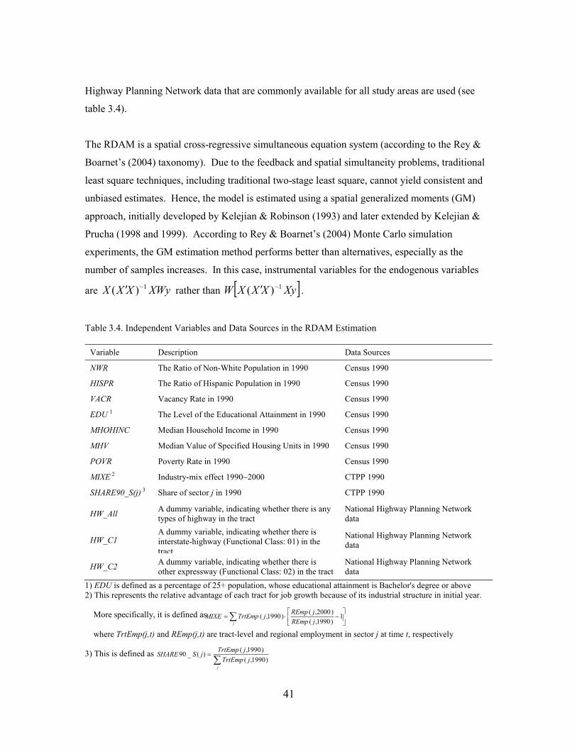
41

Highway Planning Network data that are commonly available for all study areas are used (see

table 3.4).

The RDAM is a spatial cross-regressive simultaneous equation system (according to the Rey &

Boarnet’s (2004) taxonomy). Due to the feedback and spatial simultaneity problems, traditional

least square techniques, including traditional two-stage least square, cannot yield consistent and

unbiased estimates. Hence, the model is estimated using a spatial generalized moments (GM)

approach, initially developed by Kelejian & Robinson (1993) and later extended by Kelejian &

Prucha (1998 and 1999). According to Rey & Boarnet’s (2004) Monte Carlo simulation

experiments, the GM estimation method performs better than alternatives, especially as the

number of samples increases. In this case, instrumental variables for the endogenous variables

are XWyXXX 1)( −′ rather than [ ]XyXXXW 1)( −′ .

Table 3.4. Independent Variables and Data Sources in the RDAM Estimation

Variable Description Data Sources

NWR The Ratio of Non-White Population in 1990 Census 1990

HISPR The Ratio of Hispanic Population in 1990 Census 1990

VACR Vacancy Rate in 1990 Census 1990

EDU 1 The Level of the Educational Attainment in 1990 Census 1990

MHOHINC Median Household Income in 1990 Census 1990

MHV Median Value of Specified Housing Units in 1990 Census 1990

POVR Poverty Rate in 1990 Census 1990

MIXE 2 Industry-mix effect 1990~2000 CTPP 1990

SHARE90_S(j) 3 Share of sector j in 1990 CTPP 1990

HW_All A dummy variable, indicating whether there is any types of highway in the tract

National Highway Planning Network data

HW_C1 A dummy variable, indicating whether there is interstate-highway (Functional Class: 01) in the tract

National Highway Planning Network data

HW_C2 A dummy variable, indicating whether there is other expressway (Functional Class: 02) in the tract

National Highway Planning Network data

1) EDU is defined as a percentage of 25+ population, whose educational attainment is Bachelor's degree or above 2) This represents the relative advantage of each tract for job growth because of its industrial structure in initial year.

More specifically, it is defined as

where TrtEmp(j,t) and REmp(j,t) are tract-level and regional employment in sector j at time t, respectively 3) This is defined as

∑

−⋅=

j jREmp

jREmpjTrtEmpMIXE 1

)1990,(

)2000,()1990,(

∑=

j

jTrtEmp

jTrtEmpjSSHARE

)1990,(

)1990,()(_90

42

3.3.4. Analysis Outcomes

Using the spatial GM approach, the model for each region is estimated. To obtain the final

estimation outcomes, the model specification is repeatedly modified, by excluding the

independent variables that are statistically insignificant (10%-level). Table 3.5 presents the final

estimation outcomes for Cincinnati, as an example.18

Table 3.5. An Example of the Estimation Outcomes: Cincinnati (Regulation Index = 0.16 | n = 346)

Variable Description Coefficient Standard

Error t-statistic P-value

Population Change Equation

C Intercept -673.166 246.842 -2.72712 [.006]

IWECH tiEWI ,)( ∆⋅+ ; This coefficient is EPp λθλ ⋅ 0.611898 0.135464 4.51706 [.000]

P0 1, −tiP ; This coefficient is pλ− -0.082974 0.037665 -2.20298 [.028]

IWE0 1,)( −⋅+ tiEWI ; This coefficient is pp θλ ⋅ 0.046433 0.019877 2.33598 [.019]

MHOHINC Median household income 0.021798 5.00E-03 4.35868 [.000]

MHV Median value of specified housing units -7.59E-03 2.34E-03 -3.24509 [.001]

R-squared = 0.151 | Adjusted R-squared = 0.139

Employment Change Equation

C Intercept -706.856 286.714 -2.46537 [.014]

IWPCH tiPWI ,)( ∆⋅+ ; This coefficient is PEE λθλ ⋅ 0.523736 0.116596 4.4919 [.000]

E0 1, −tiE ; This coefficient is Eλ− -0.142054 0.026769 -5.30675 [.000]

IWP0 1,)( −⋅+ tiPWI ; This coefficient is EE θλ ⋅ 0.099835 0.034612 2.88443 [.004]

MIXE Industry mix effect 0.527012 0.140346 3.7551 [.000]

SHARE90_S2 Share of Construction Sector -2395.78 1131.42 -2.11749 [.034]

SHARE90_S7 Share of Finance, Insurance, and Real Estate

Sector 3111.51 1445.52 2.15252 [.031]

HW_C1 Interstate highway dummy 351.369 135.519 2.59276 [.010]

R-squared = 0.192 | Adjusted R-squared = 0.175

Some of the estimated coefficients, presented in table 3.5, need to be explained. First, the

negative coefficient of MHV may suggest that a greater amount of housing costs tend to push

people out of the area. The positive value of SHARE90_S7’s coefficient can be interpreted as the

18 It needs to be noted that the low values of r-squared, to some extents, are attributable to the model design in which population or employment changes (as opposed to population and employment levels) are dependent variables. In fact, most studies, specifying the RDAM in this way, report r-squared lower than 0.40. Another reason may be a limited number of independent variables considered due to the data availability problem.

43

attracting force of the financial sector. Finally, the negative coefficient of SHARE90_S2 can be

attributed to the temporary construction jobs in the field. In other words, the areas showing a

high share of construction sector in 1990 tend to show a job loss after the completion of

development projects which would not last a decade (i.e. from 1990 to 2000).

Like many other studies employing the RDAM, for some metropolitan areas, statistically

insignificant estimates for key variables are often found: IWECH, P0, and IWE0 in population

change equation and IWPCH, E0, and IWP0 in employment change equation. This may happen,

because all location factors cannot be considered due to the data availability problem. According

to Boarnet et al. (2005), the performance of this model can be improved by considering micro

land use information as explanatory variables. Also, Mulligan and others’ (1999) experiment

suggests that better estimation outcomes would be obtained, if 5 years or shorter time spans are

used in the analysis. However, a shorter time span or sufficient explanatory variables could not

be used in this study, because tract-level population and employment data only available for

decennial years; and the information for many other factors at this level is unavailable.

As mentioned above, in these cases of invalid estimation outcomes, it is impossible to determine

valid values of the four parameters of interest. Therefore, the outcomes of these regions are not

considered. The estimation outcomes of the key coefficients in valid cases are summarized in

table 3.6.

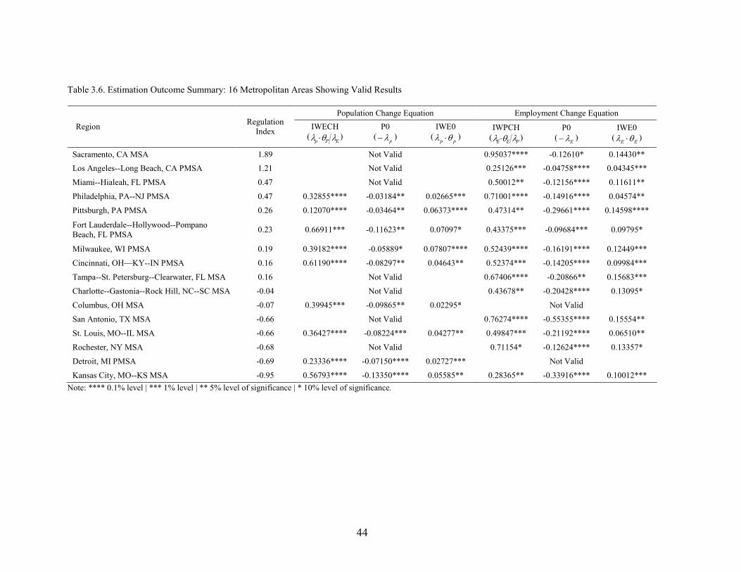
44

Table 3.6. Estimation Outcome Summary: 16 Metropolitan Areas Showing Valid Results

Population Change Equation Employment Change Equation

Region Regulation

Index IWECH

(EPp λθλ ⋅ )

P0

(pλ− )

IWE0

(pp θλ ⋅ )

IWPCH

(PEE λθλ ⋅ )

P0

(Eλ− )

IWE0

(EE θλ ⋅ )

Sacramento, CA MSA 1.89 Not Valid 0.95037**** -0.12610* 0.14430**

Los Angeles--Long Beach, CA PMSA 1.21 Not Valid 0.25126*** -0.04758**** 0.04345***

Miami--Hialeah, FL PMSA 0.47 Not Valid 0.50012** -0.12156**** 0.11611**

Philadelphia, PA--NJ PMSA 0.47 0.32855**** -0.03184** 0.02665*** 0.71001**** -0.14916**** 0.04574**

Pittsburgh, PA PMSA 0.26 0.12070**** -0.03464** 0.06373**** 0.47314** -0.29661**** 0.14598****

Fort Lauderdale--Hollywood--Pompano Beach, FL PMSA

0.23 0.66911*** -0.11623** 0.07097* 0.43375*** -0.09684*** 0.09795*

Milwaukee, WI PMSA 0.19 0.39182**** -0.05889* 0.07807**** 0.52439**** -0.16191**** 0.12449***

Cincinnati, OH—KY--IN PMSA 0.16 0.61190**** -0.08297** 0.04643** 0.52374*** -0.14205**** 0.09984***

Tampa--St. Petersburg--Clearwater, FL MSA 0.16 Not Valid 0.67406**** -0.20866** 0.15683***

Charlotte--Gastonia--Rock Hill, NC--SC MSA -0.04 Not Valid 0.43678** -0.20428**** 0.13095*

Columbus, OH MSA -0.07 0.39945*** -0.09865** 0.02295* Not Valid

San Antonio, TX MSA -0.66 Not Valid 0.76274**** -0.55355**** 0.15554**

St. Louis, MO--IL MSA -0.66 0.36427**** -0.08224*** 0.04277** 0.49847*** -0.21192**** 0.06510**

Rochester, NY MSA -0.68 Not Valid 0.71154* -0.12624**** 0.13357*

Detroit, MI PMSA -0.69 0.23336**** -0.07150**** 0.02727*** Not Valid

Kansas City, MO--KS MSA -0.95 0.56793**** -0.13350**** 0.05585** 0.28365** -0.33916**** 0.10012***

Note: **** 0.1% level | *** 1% level | ** 5% level of significance | * 10% level of significance.

45

Using the valid estimation outcomes, the parameter values are determined for individual

metropolitan areas. Then, they are related to the regulation index to see how they differ across

regions with different regulation levels. Figures 3.7 through 3.10 demonstrate the relationships

between the region-wide land use regulation index and the four parameters.

Relationship between Regulation Index and Household Mobility

y = -0.0374x + 0.0745

R2 = 0.3118

y = -0.0332x + 0.2185

R2 = 0.1149

0

0.05

0.1

0.15

0.2

0.25

0.3

0.35

0.4

-1.5 -1 -0.5 0 0.5 1 1.5 2 2.5

Regulation Index

Household Mobility

from Pop Change Eq

from Emp Change Eq

Linear (from Pop Change Eq)

Linear (from Emp Change Eq)

Correlation = -0.339

Correlation = -0.558

Figure 3.7. Relationship between Regulation Index and Household Mobility (

pλ )

Relationship between Regulation Index and the Magnitude of Job Effect

y = 0.5367x + 0.8105

R2 = 0.2811

0

0.2

0.4

0.6

0.8

1

1.2

1.4

1.6

1.8

2

-1.5 -1 -0.5 0 0.5 1 1.5 2 2.5

Regulation Index

Magnitude of Job Effect

Correlation = 0.530

Figure 3.8. Relationship between Regulation Index and the Magnitude of Job Effect (

pθ )

46

Relationship between Regulation Index and Business Mobility

y = 0.0748x + 0.1622

R2 = 0.0687

y = -0.0944x + 0.2128

R2 = 0.3203

0

0.1

0.2

0.3

0.4

0.5

0.6

-1.5 -1 -0.5 0 0.5 1 1.5 2 2.5

Regulation Index

Business Mobility

from Pop Change Eq

from Emp Change Eq

Linear (from Pop Change Eq)

Linear (from Emp Change Eq)

Correlation = -0.566

Correlation = 0.262

Figure 3.9. Relationship between Regulation Index and Business Mobility (

Eλ )

Relationship between Regulation Index and the Magnitude of Population Effect

y = 0.233x + 0.6536

R2 = 0.3356

0

0.2

0.4

0.6

0.8

1

1.2

1.4

-1.5 -1 -0.5 0 0.5 1 1.5 2 2.5

Regulation Index

Magnitude of Population Effect

Correlation = 0.579

Figure 3.10. Relationship between Regulation Index and the Magnitude of Population Effect (

Eθ )

Although the valid outcomes are obtained only for a limited number of study regions, this set of

the results, as it stands, suggests that a more regulated metropolitan area tends to have:

1) a lower level of household mobility (figure 3.7);

2) a greater magnitude of job effect on household location choice (figure 3.8);

47

3) mixed outcomes regarding business mobility (figure 3.9)19;

4) a greater magnitude of population effect on business location choice (figure 3.10)

Overall, at least, the results may suggest that the alternative hypotheses, particularly a smaller

magnitude of job effect on household location choice and a smaller magnitude of population

effect on business location choice, may not be the case. Rather, intraregional population and

employment may not be well interconnected in regulated metropolitan areas due to the lower

household mobility, even though household and businesses may want to locate closer to each

other, consistent with the hypothesis of this research.

3.4. Summary & Discussion

In this study, I attempt to examine whether or not land use regulations prevent people from

responding to new job conditions or other location factors in a timely manner, by analyzing how

intraregional population-employment interaction varies by regions having different degrees of

land use regulations. Through the correlation analysis, the results revealed that highly regulated

metropolitan areas are more likely to show lower levels of correlation between intraregional

population and employment changes and increasing mean commuting time between 1990 and

2000. Also, the estimation outcomes of the spatial econometric analysis, using a regional

disequilibrium adjustment model, suggest that household mobility is lower in more regulated

areas than relatively less regulated regions, consistent with the hypothesis.

However, the findings rest on limited analysis outcomes and thus are not conclusive. In the

correlation analysis, various other factors that may influence the PCh-ECh correlation or

commuting time changes are not controlled. Also, in the spatial econometric analysis, valid

estimation outcomes were available for only some metropolitan areas. In particular, many highly

19 First, the estimated coefficients of employment change equations indicate a poorer mobility of business in a highly regulated metropolitan area. This can be explained by 1) that commercial-industrial development is also much more regulated in the regions having high values of the index, although the index primarily represents residential land use regulations or 2) that residential land use regulations affects property market, as a whole, so that business mobility is influenced. However, the opposite relationship (i.e. a higher level of business mobility in the region with higher regulation index) is derived from the estimates in the population change equations.

48

regulated regions cannot be considered in the interpretation of the outcomes, due to the problem

of insignificant estimates.

This study is also limited in the sense that aggregated population and employment, as opposed to

households by group and businesses by sector, are modeled. As well presented in housing and

migration literature, household location choice heavily depends on many demographic (e.g.

household size, age, children, etc) and economic (income level, one-earner vs. two-earner

households, etc) factors. A great deal of heterogeneity also exists in business location decision-

making, because of the differences in production recipes, suppliers, and customers. This issue of

aggregation is clearly important as some income groups have no limitations while, for lower

income groups, land use regulation may generate significant impediments to re-location.

Also, the 10 year time span of this analysis may not be ideal for obtaining precise values of

residential or business location mobility, although this is somewhat inevitable due to the limited

availability of disaggregated-level data. Furthermore, the direction of causality has not been

tested especially whether land use regulations are really responsible for the observed inclinations

of highly regulated regions, such as the relatively weak intraregional population-employment

connections and increasing mean commuting time.

Nevertheless, by showing some empirical analysis outcomes corresponding to the hypothesis, the

present research may be able to provide land use planners or policy makers with a meaningful

caution about their regulatory actions. It is probable that strict regulatory barriers make local

housing markets less flexible and dampen household mobility and that may result in the reduced

utility of residents and further reduced profits of businesses. Moreover, the affected intraregional

population-employment interaction may generate longer commuting times, distances and costs

and distort the spatial structure of the region. However, the results should not be interpreted to

imply that planners’ intervention in the land development process is harmful. Rather, it is a claim

for more informed decision-making as well as a balanced view of the benefits and costs of land

use regulations.

49

4. LAND USE PLANNING AS INFORMATION PRODUCTION & EXCHANGE

4.1. Introduction

Government interventions in land use planning have been traditionally justified from an economic

perspective as well as by political theories and environmental rationales. In particular, welfare

economic theory, combined with the demonstration of some market failures that can be traced to

externalities and public goods problems, has been mainly used for the justification. As explained

in the literature review, for example, Bailey (1959) noted that the welfare level of land owners

can be raised by appropriate land use controls that eliminate existing negative externalities. He

argued that this welfare increase is a major benefit of land use planning. Davis (1963) considered

the ideal zoning restriction as a state “under which external diseconomies are simply eliminated”

(p.383), so that land use becomes more economically efficient. In addition to these early studies,

many others have justified government action in the form of land use planning and regulation, in

a similar way – i.e. using welfare economics per se. The studies would include Gardner (1977)

and Moore (1978)’s work that focus on the issue of public goods as well as Lee’s (1981) article,

Land Use Planning as a Response to Market Failure, where the regulations of the land market

process are advocated. Furthermore, such claims have been supported by many empirical studies

that demonstrate the virtual existence of negative externalities in the context of uncontrolled land

use (see e.g. Stull 1975; Lafferty & Frech 1978: Burnell 1985) or the benefits of environmental

amenities, preserved by the regulations (see e.g. Correll et al. 1978; Spalatro & Provencher 2001).

However, there are some critical shortcomings of the justification on the basis of welfare

economic theory and the existence of typical market failures. First, because it is a static

framework, the welfare economics approach has limited usefulness in dealing with land use and

development issues, which are dynamic and irreversible in nature (see e.g. Ohls & Pines 1975;

Arnott & Lewis 1979; Capozza & Helsley 1990). In addition, based on the government vs.

market dichotomy, this approach only considers the possible benefits of land use regulation,

which is just an end-product from a series of land use planning practices, in addressing market

failures and, consequently, achieving a higher level of the efficiency in land allocation among

50

various uses.20 It neglects the other benefits of the entire land use planning process, particularly

the aspect of information production and exchange. Land use planning practice produces

information relevant to land use as well as facilitates the exchange of information, and

consequently may reduce uncertainties and help the decision-making of various actors involved in

the process of land development (Friend & Jessop 1969; Schaeffer & Hopkins 1987; Knaap et al.

1998). In other words, land use planning practice could bring some economic benefits, even if

the final decision – that may or may not be a regulatory action – does not achieve a higher level

of the efficiency in allocation.

The importance of this contribution of land use planning (i.e. information production and

exchange) has been emphasized by studies that draw on transaction-cost economic (TCE) theory.

For instance, as mentioned in the literature review, Alexander (1992, 1994, and 2001) claimed

that land markets generally bear substantial uncertainties and unnecessary transaction costs, thus

requiring government intervention which reduces those costs by providing valuable information

more efficiently. Dawkins (2000) also highlighted this point by arguing that land use planning

practices or regulatory interventions by government can effectively lower uncertainties as well as

transaction costs involved in land development processes.

Notwithstanding these important theoretical discussions, empirical studies that validate the

theoretical suppositions are scarce, so that little is known about the real-world effect of land use

planning on uncertainties and transaction costs.21 The present study attempts to fill this gap.

Here, an examination is made to see whether or not land use planning actually contributes to

reducing the level of uncertainty in land markets as suggested by the TCE-based claims. Rather

than considering various kinds of uncertainties in multi-stage land development and land use

processes, the focus will be on a particular case, namely the urban fringe land markets where

farmland owners are faced with uncertainty regarding the timing of potential land development

for urban uses. Based on an understanding of the strategic behavior of farmland owners under

20 In fact, land use planning is different from the regulatory behavior of government. As noted in chapter 2, Hopkins (2001) makes this point clear by explaining that “Regulations [are] … enforceable assignment and reassignment of rights. Regulations affect the scope of permissible actions. Plans … provide information about interdependent decisions in relation to expected outcomes but these plans do not determine directly the scope of permissible actions” (p.9-10). 21 There are a few empirical studies which examine whether plans or information contained in the plans, as opposed to the regulatory actions, have effects on decision-making of economic agents (See e.g. Talen 1996a and 1996b; Knaap et al. 2001). But they do not test the validity of the TCE-based justification of land use planning.

51

uncertainty, the validity of the TCE-based justification is tested by conducting an exploratory

spatial data analysis first followed by an MSA-level statistical analysis.

The remainder of this chapter is structured as follows. Section 4.2 briefly discusses the choice

problems and decision making of farmland owners for using urban fringe areas until the uncertain

time point of development and the consequences if land use planning, particularly the urban

growth boundary (UGB), reduces the uncertainty as suggested by the TCE-based argument. In

section 4.3, the farmland use pattern in Oregon is explored as an example to see how farmland

owners may exploit or respond to the information in the UGB. Section 4.4 presents a regression

analysis designed to measure the effect of the land use planning practice (i.e. UGB establishment)

on uncertainty reduction, by using the data of 82 single-county MSAs across states. A

concluding section, where the findings are summarized and discussed, completes the paper.

4.2. Behaviors of Farmland Owners & the Establishment of UGBs

Farmland conversion to developed land is a general trend across the states. According to the

1997 National Resources Inventory prepared by USDA Natural Resources Conservation Service

(NRCS), approximately 15 million acres of cropland, pastureland, and rangeland had been

developed for urban uses between 1982 and 1997 (table 4.1). In particular, the farmland at the

urban fringe has been the main target of the new development.

Under this situation with a high pressure or probability of conversion, the farmland owners at the

urban fringe are facing two types of important decision-making every year. The first decision to

be made is a discrete choice on whether to subdivide their lots and convert them for urban uses

right now or keep using the land for agricultural production at least for the current year. 22 The

farmland owners, who seek to maximize their profits, may develop their land, if and only if they

conclude that the conversion at this time brings a greater value in terms of the future stream of

returns than all other alternatives (i.e. no conversion or conversion at all other time points),

22 This (first) decision-making process has been discussed more intensively by many studies on land use changes, such as Bockstael (1996), Irwin & Geoghegan (2001), and Segerson et al. (2006).

52

considering the profitability of continuing agricultural production activities and the expected

returns of the development in future.23

Table 4.1. Land Use Change between 1982 and 1997 in the United States (Unit: 1000 acres)

Land cover/use in 1997

Land

cover/use

in 1982 Cropland CRP land

Pasture-land

Range-land

Forest land

Other rural land

Developed land

Water areas & federal

land

1982

total

Cropland 350,265 30,412 19,269 3,659 5,607 3,159 7,098 1,485 420,954

Pasture-land

15,347 1,330 92,088 2,568 14,091 1,619 4,230 733 132,006

Rangeland 6,968 729 3,037 394,617 3,022 1,703 3,281 3,383 416,739

Forest land 2,037 129 4,168 2,099 380,343 1,755 10,279 2,528 403,338

Other rural land

1,387 93 1,014 719 2,768 42,713 727 228 49,648

Developed Land

197 1 79 111 227 12 72,619 1 73,246

Water areas & federal

land 798 3 337 2,204 898 181 18 443,761 448,198

1997 total 376,998 32,696 119,992 405,977 406,955 51,142 98,252 452,118 1,944, 130

Source: Table 5, 1997 National Resources Inventory, USDA NRCS

The second decision-making option comes when the farmland owners do not convert their land at

this time. If this is the case, a set of decisions need to be made on how to use the land without

development, until the time comes for them to opt for development. In other words, they decide

the items of production, the number of workers to be hired, and the level of capital investment in

order to maximize the profits while using their land for the agricultural production.24

These decisions, particularly production item choice and capital investment, are highly affected

by the farmland owners’ prediction of the timing of land development in the future. Because

cultivating certain items requires a longer period of operation or a larger amount of sunk costs to

23 The assumption of farmland owners’ profit maximization does not mean the homogeneity of the owners. There is a significant amount of variance by individuals in this decision making, as reported by Barnard & Butcher (1989) and many others. 24 It is possible not to use the land for any purposes. However, since there is a considerable amount of financial advantages while using land for agricultural activity in the U.S., the owners may tend to use or pretend to use the land for agricultural production.

53

make an acceptable amount of profit, they are reluctant to choose those items if there is an

enhanced probability of development of his/her parcels within the next few years. Also, since

capital investment is generally irreversible, they are less likely to put capital in agricultural

production if they think the invested capital may not be fully utilized in terms of the return on

investment. In this case, they may give up the improvement of irrigation or other supporting

system or use existing machinery and equipment rather than buying new ones, even if new

investment is required for the optimal agricultural production from a long-term perspective.

These influences of development timing have been investigated by some studies on agricultural

production, although consideration has not been given to the role of land use planning. For

example, Lopez et al. (1988) conducted a longitudinal analysis to examine how agricultural

production in New Jersey is affected by the degree of suburbanization, measured by population in

nonurban counties, and found that fruit and livestock production is discouraged by

suburbanization. Their analysis outcomes also suggest that agricultural production tends to

become more labor intensive (i.e. declining capital and land inputs), as the region is more

suburbanized.

The Farm & Ranch Irrigation Survey, conducted by the USDA National Agricultural Statistics

Service (NASS), also provides some evidence of this behavioral pattern. As a part of the survey,

the farmers were asked about the “barriers to making improvements to reduce energy use or

conserve water”. According to the survey, 5~8 percent of respondents in the entire U.S.

answered “will not be farming this operation long enough to justify improvements” in response to

the question, “why not invest in improvements?” (table 4.2).

54

Table 4.2. Farm & Ranch Irrigation Survey Outcomes: Barriers to the System Improvements

2008 Survey 2003 Survey

Farms % Farms %

1."Investigating improvements not a priority" 46,825 21.7% 9,055 8.0%

2. "Risk of reduced yield or poor crop quality" 18,578 8.6% 9,818 8.7%

3. "Physical field/crop condition limit system improvements"

20,888 9.7% 8,951 7.9%

4. "Improvements will not reduce costs enough to cover installation costs"

33,725 15.7% 21,304 18.8%

5. "Cannot finance improvements" 37,512 17.4% 20,122 17.7%

6. "Landlord will not share in cost" 6,815 3.2% 8,194 7.2%

7. "Uncertainty about future availability of water" 19,536 9.1% 13,790 12.2%

8. "Will not be farming this operation long enough to justify improvements"

17,280 8.0% 6,204 5.5%

9. "Other" 14,272 6.6% 15,995 14.1%

Total 215,431 100.0% 113,433 100.0%

Source: Table 41, 2008 Farm & Ranch Irrigation Survey Report Note: Respondents are allowed to choose more than one barrier to improvement. Here, “Total” is the number of all responses, as opposed to the number of respondents.

In the real world, the farmland owners’ prediction of development timing and the following

decisions are made with uncertainty. Under a higher level of the uncertainty, the owners cannot

predict the exact timing of land development and attach low values of confidence in their

predictions. This may raise the risk of over-investment and alter the item choices and capital

investment decision-making for the agricultural production: i.e. the farmland owners are less

likely to grow the items with a greater amount of sunk costs and are less likely to increase or

continue irreversible investment.

According to the argument of TCE-based justification of planning, these kinds of uncertainties

can be reduced with relevant information, produced and exchanged through effective land use

planning practices. Particularly, the uncertainty in the urban fringe land markets could be

lowered by the establishment of an UGB, a widely used land use planning practice related to such

fringe areas.25 Although the practice qualitatively and administratively differs across regions (see

e.g. Gale 1992; Innes 1992), through the UGB establishment processes, local and regional

government bodies typically 1) conduct population projections, 2) determine the future demand

25 In the United States, an UGB was first adopted by Lexington, Kentucky in 1958 (Nelson & Duncan 1995). As of 1998, more than a hundred regions establish UGBs (Staley et al. 1999). Furthermore, Oregon, Washington, and Tennessee enacted state-level legislation that mandates local and regional government to do this work and to incorporate the UGBs into their comprehensive plans.

55

of new development, 3) investigate suitable or desirable locations for new development, and then

4) draw the boundary, as a proposal (Anderson 1999). In addition, like many other planning

processes, the proposed boundary is publicized and reviewed by various actors at public hearings

or some other forms of public engagement where the ideas and information related to future

development are exchanged. In the end, an UGB, as a final product that reveals the expected

expansion of developed areas for upcoming 20 years or some other periods of time, is established.

From the perspective of farming, the UGB is not a regulation binding item choice, investment, or

detailed operation. Rather, the boundary is valuable information that helps individual farmland

owners obtain a better sense about the probable timing for development of their land, as

characterized by Knaap (1985). In addition to the UGB itself, population projection, new

development demand estimation, site investigation, and opinions of other actors at the place of

collaborative planning may also inform the farmland owners, who make their own decisions

looking forward.

4.3. Spatial Data Analysis

Do uncertainties exist in urban fringe land markets? Does the UGB establishment really inform

farmland owners in the sense of reducing uncertainty and thus transactions costs? In this section,

a data analysis will be conducted using the case of Oregon, in order to explore 1) whether or not

there are any notable relationships between farmland use patterns and the established UGBs and

2) whether the demonstrable relationships suggest a real contribution of the UGB establishment

practice to the uncertainty reduction.

Given that disaggregated-level investment data or other measurements representing the

uncertainty level are not available, the only option is to use the farmland use pattern (i.e. what

items are grown at particular location points), along with the knowledge about the characteristics

of various items, such as the minimum period of operation for the profit and the required level of

sunk costs for production. Although farmland use is determined by many other factors, such as

physical characteristics, the farmer’s capability and preferences, and so on, certain types of

56

agricultural production, with greater time and sunk cost requirements, may be less likely to

appear where land development is expected to happen soon.

4.3.1. Method & Data

The main task of this spatial analysis is to explore how the farmland use patterns vary across

space. To do this, above all, the urban fringe areas of interest are divided according to the

distance to the cities. This is accomplished by using the boundaries of the Census’s Urbanized

Area and Urban Cluster, which well represent the borders of the densely developed territories,

rather than using the administrative city limits. In other words, the fringe areas are first classified

into six categories: 1) between the border and 0.5 mile buffer, 2) 0.5~1.0 mile area, 3) 1.0~1.5

mile area, 4) 1.5~2.0 mile area, 5) 2.0~2.5 mile area, and 6) 2.5~3.0 mile area. Although this way

of space division is useful for capturing the relationship between the farmland use pattern and the

proximity to the cities that had been well discussed in the land use analysis of von Thunen (1826),

the buffer width (i.e. 0.5 mile) may be too large to consider the uncertainty and thus the full

impact of the UGB. Therefore, the first category (i.e. between the border and 0.5 mile buffer) is

sub-divided to 0.1 mile buffer zones: i.e. 1-a) between the borders and 0.1 mile buffers, 1-b)

0.1~0.2 mile area, 1-c) 0.2~0.3 mile area, 1-d) 0.3~0.4mile area, and 1-e) 0.4~0.5 mile area

(figure 4.1). Then, the zones are further classified by overlaying the UGBs. As a result, the areas

Within vs. Out of the UGBs are differentiated, even though the areas have the same distance to

the cities. Finally, by using the Tabulate Area function in ArcGIS as well as high-resolution land

use data, the farmland use patterns in each type of zones are measured in terms of the land use

mix.

57

Figure 4.1. Space Division and Land Uses: The Case of Eugene-Springfield MSA (Lane County, OR)

58

This method of analysis is applied to the state of Oregon where the UGBs have long been

implemented. The availability of GIS data for the analysis is another reason of the choice. The

Oregon Geospatial Enterprise Office provides the UGB shapefiles for recent years; 2007 version

is used for this analysis. For the land use information, the 2007 Cropland Data Layer (CDL) for

Oregon made by USDA NASS is employed. Because the original CDL adopts a very detailed

land use type classification, the uses are aggregated into 10 categories for the analysis, as

presented in figure 4.1. For the boundaries of Census’s Urbanized Area and Urban Cluster, the

Census TIGER (Topologically Integrated Geographic Encoding and Referencing) data are

employed.

4.3.2. Analysis Outcomes

Table 4.3 shows how the land use mixes differ across 0.5-mile buffer zones from the urbanized

area borders in Oregon. Also, the varying farmland patterns are graphically demonstrated in

figure 2, where each item’s share of the sum of all croplands is plotted over the distance to the

cities.

The general trends of farmland use across space are well revealed here. Small grains, such as

corn, rice, and wheat, are more likely to be grown, as the distance to the cities goes up. In

contrast, consistent with our intuition based the lessons from von Thunen, tree fruits and nuts as

well as potatoes, onions, peas, etc, bearing larger per distance transportation costs, tend to be

grown more in the areas with higher accessibility to the cities. The pattern of Fallow/Idle

Cropland (i.e. declining share over distance) is interesting. One possible explanation could be

traced to the farmland owner’s strategic behavior, that is they are less likely to improve the soil

quality by letting their land lie fallow near city edges, because they feel that the land will be

developed soon, so that agricultural production will not continue long enough.26

26 Alternatively, this may happen, because this type of land use (i.e. Fallow / Idle Cropland) is highly associated with small grains, showing the same declining pattern over distance, rather than other items.

59

Table 4.3. Land Use Patterns by 0.5-Mile Buffer Zones in Oregon

Borders ~0.5mile

0.5~1.0 mile

1.0~1.5 mile

1.5~2.0 mile

2.0~2.5 mile

2.5~3.0 mile

Percentage to total

Small grains, including corn, rice, barley, wheat, etc

1.7% 2.4% 2.6% 2.7% 2.7% 2.8%

Hays, including rye, oats, canola, etc 1.2% 1.5% 1.7% 1.7% 1.8% 1.6%

Other crops, including potatoes, onions, peas, etc

1.6% 2.0% 1.7% 1.7% 1.9% 1.6%

Tree fruits and tree nuts 0.6% 0.6% 0.7% 0.6% 0.5% 0.5%

Fallow/Idle cropland 0.4% 0.5% 0.6% 0.8% 0.7% 0.8%

Developed 21.0% 12.2% 10.2% 9.1% 8.4% 7.4%

Grassland, including seed/sod grass, herbs, clover/wildflowers, etc

28.2% 30.2% 29.8% 28.7% 28.1% 27.2%

Forest, woodland, and shrubland 32.4% 40.4% 43.3% 46.7% 49.2% 51.8%

Barren 0.9% 0.9% 0.9% 0.8% 0.7% 0.8%

Water and wetlands 12.0% 9.2% 8.4% 7.2% 6.1% 5.6%

Percentage to the sum of croplands

Small grains, including corn, rice, barley, wheat, etc

30.8% 34.0% 35.3% 36.0% 35.7% 38.2%

Hays, including rye, oats, canola, etc 21.7% 21.5% 23.7% 22.8% 23.4% 21.5%

Other crops, including potatoes, onions, peas, etc

30.0% 27.9% 23.6% 23.0% 24.6% 22.3%

Tree fruits and tree nuts 10.9% 8.9% 9.2% 8.2% 6.3% 6.2%

Fallow/Idle cropland 6.6% 7.7% 8.1% 10.0% 10.0% 11.7%

60

0.0%

5.0%

10.0%

15.0%

20.0%

25.0%

30.0%

35.0%

40.0%

45.0%

50.0%

Border~0.5mile 0.5~1.0mile 1.0~1.5mile 1.5~2.0mile 2.0~2.5mile 2.5~3.0mile

Small grains, including corn, rice, barley, wheat, etc

Hays, including rye, oats, canola, etc

Other crops, including potatoes, onions, peas, etc

Tree fruits and tree nuts

Fallow/Idle cropland

Figure 4.2. Farmland Use Patterns in Oregon’s Urban Fringe Areas

The farmland land use patterns within the 0.5 mile buffer, where a higher level of uncertainty

may exist, are investigated in detail by using the 0.1 mile buffer zones and UGBs. Table 4.4

presents the patterns over distance with respect to UGBs in terms of percentage to the sum of

croplands.

Above all, attention needs to be paid to the pattern of tree fruits and tree nuts. As found in the

previous analysis, generally this item is more likely to occupy the areas close to the cities.

However, since it bears a larger amount of sunk costs, thereby profitable when the operation

continues for a certain period of time, the item may be less likely to appear where development is

expected to occur in few years or development timing is very uncertain. If the UGBs really

inform the farmland owners and help their decision-making as argued by the TCE-based

justification of land use planning practices, we will find the distinct difference in this land use

type between Within-UGBs zones and Out-of-UGBs zones, although the difference does not

necessarily mean the TCE-based argument is valid.

61

Table 4.4. Land Use Patterns within 0.5-Mile Buffer in Oregon

Borders ~0.1mile

0.1~0.2 mile

0.2~0.3 mile

0.3~0.4 mile

0.4~0.5 mile

Percentage to the sum of croplands (Within UGBs)

Small grains, including corn, rice, barley, wheat, etc

23.8% 27.8% 36.4% 37.9% 43.7%

Hays, including rye, oats, canola, etc 20.6% 17.7% 16.1% 14.4% 11.7%

Other crops, including potatoes, onions, peas, etc

37.5% 35.0% 32.1% 31.9% 29.5%

Tree fruits and tree nuts 9.1% 9.9% 7.6% 7.3% 6.1%

Fallow/Idle cropland 9.1% 9.5% 7.9% 8.5% 9.0%

Percentage to the sum of croplands (Out of UGBs)

Small grains, including corn, rice, barley, wheat, etc

28.3% 28.8% 30.1% 30.7% 32.9%

Hays, including rye, oats, canola, etc 19.8% 22.3% 23.7% 23.3% 22.4%

Other crops, including potatoes, onions, peas, etc

30.9% 30.3% 30.0% 29.6% 27.3%

Tree fruits and tree nuts 14.3% 12.3% 10.6% 10.5% 10.5%

Fallow/Idle cropland 6.8% 6.2% 5.7% 5.9% 6.8%

It needs to be noted that the item choice in reality is path-dependent, thus more complicated than

the description here. Suppose a farmland owner who has grown tree fruits in his land a long time

before the emergence of development pressure. Because the trees and other structures for the

operation are sunk costs, he may continue to cultivate the fruits rather than changing the item

with a certain (probably low) level of investment in maintenance, even if his land will be

developed soon. This results in the production of the tree fruits in the farms with high

development probability or uncertainty, in contrast to the noted expectation. However, new fruit

production may be less likely to locate in these farms. It may tend to go to the sites where the

need for accessibility and the required operation period for profits are satisfied. If an UGB

functions as anticipated, it provides valuable information for this site selection. As a result, the

fruit items will be more likely to appear out of UGB, ceteris paribus.

The outcomes of the detailed investigation suggest this is the case. It is apparent that tree fruits

and tree nuts is much important in the farmlands outside of the UGBs (table 4.4 and figure 4.3).

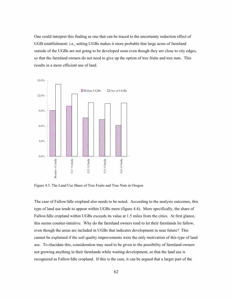
62

One could interpret this finding as one that can be traced to the uncertainty reduction effect of

UGB establishment: i.e., setting UGBs makes it more probable that large acres of farmland

outside of the UGBs are not going to be developed soon even though they are close to city edges,

so that the farmland owners do not need to give up the option of tree fruits and tree nuts. This

results in a more efficient use of land.

0.0%

3.0%

6.0%

9.0%

12.0%

15.0%

Border~0.1mile

0.1~0.2mile

0.2~0.3mile

0.3~0.4mile

0.4~0.5mile

Within UGBs Out of UGBs

Figure 4.3. The Land Use Share of Tree Fruits and Tree Nuts in Oregon

The case of Fallow/Idle cropland also needs to be noted. According to the analysis outcomes, this

type of land use tends to appear within UGBs more (figure 4.4). More specifically, the share of

Fallow/Idle cropland within UGBs exceeds its value at 1.5 miles from the cities. At first glance,

this seems counter-intuitive. Why do the farmland owners tend to let their farmlands lie fallow,

even though the areas are included in UGBs that indicates development in near future? This

cannot be explained if the soil quality improvements were the only motivation of this type of land

use. To elucidate this, consideration may need to be given to the possibility of farmland owners

not growing anything in their farmlands while waiting development, so that the land use is

recognized as Fallow/Idle cropland. If this is the case, it can be argued that a larger part of the

63

urban fringe lands (i.e. the areas outside of the UGBs) is more intensively used as a direct

consequence of the establishment of the UGB that informs the farmland owners that their parcels

are not going to be developed soon.

0.0%

3.0%

6.0%

9.0%

12.0%

Border~0.1mile

0.1~0.2mile

0.2~0.3mile

0.3~0.4mile

0.4~0.5mile

Within UGBs Out of UGBs

Figure 4.4. The Land Use Share of Fallow / Idle Cropland in Oregon

4.4. Regression Analysis

The previous section explored the UGB’s effect in the urban fringe land markets by using high-

resolution land use data. In this section, an examination will be made of the possible contribution

of UGB establishment to uncertainty reduction and to derive a more generalized conclusion on

the validity of TCE-based justification of land use planning practice by conducting a statistical

analysis with single-county MSAs as units of analysis. The idea, explained in section 4.2, is that

the farmland owners may tend to increase the value of investments if the level of the uncertainty

associated with the timing of development of their farmlands is reduced, as they would then be

faced with a lower risk metric with respect to wasting irreversible investments. In other words,

64

the value of investments may to some extent represent the uncertainty level. If the UGB

establishment really reduces the uncertainty consistent with TCE-based arguments, then there

should be a positive effect of UGBs on agricultural investment when other factors are properly

controlled.

4.4.1. Model

For the simplicity, suppose that the agricultural production exhibits constant returns to scale with

a Cobb-Douglas form.

γβαφ LKSX ⋅⋅⋅= (4-1) 1=++ γβα

where X is the output of agricultural production, S is land input, K is capital investment, and

L is labor force for the production. Coefficient φ is the technology parameter, which represents

the efficiency level in production. α , β , and γ are cost share parameters for land, capital, and

labor force, respectively.

In this setting, the optimal levels of land and capital input, that minimizes the production cost for

a certain amount of production, are

Sp

XpS

⋅⋅=α*

(4-2) Kp

XpK

⋅⋅=β*

(4-3)

where p , Sp , and

Kp are the price of final farm product, land, and capital, respectively.

From the equation (4-2) and (4-3), the optimal level of per acre capital investment can be derived,

as below.

K

S

S

K

p

p

pXp

pXp

S

K

S

K

⋅⋅

=⋅⋅

⋅⋅

==

αβ

α

β

*

**

(4-4)

Then, by taking log on both sides of the equation (4-4), a linear form, which is a basis of the

model making, can be obtained.

( ) )log()log()log()log(log*

βα +−−= KS ppS

K (4-5)

65

The equation (4-5) implies that per acre capital investment is a function of land price (Sp ),

capital price (Kp ), and the two cost share parameters (α and β ), in the assumed situation of

agricultural production. Among the four determinants in this equation, land price is the most

important factor to explain the level of per acre capital investment in an empirical analysis using

cross sectional data like this study, since it varies significantly across regions. The two cost share

parameters, representing the character of agricultural production, are also influential ones.

Because these parameters are item- and region-specific, this study tries to capture the influence of

these factors on per acre capital investment by including additional explanatory variables, such as

individual items’ shares in terms of sales and the regional control dummies. Unlike land price

and the two cost share parameters, capital price is assumed to be a constant, since its variance

across regions in the U.S. is not available.

In addition to the above variables, several more factors should be included to precisely explain

the real per acre capital investment and correctly examine the effect of UGB establishment

practice on investment level. Since the farmland owners are able to adjust the level of capital

investment responding to the relative prices of other inputs (i.e. they can substitute capital with

other inputs and vice versa) for the cost minimization as well, here, the price of labor (i.e. wage

level of hired farm labor), which varies by region most significantly, is included in the list of the

independent variables. Also, because the economies of scale may exist in the real agricultural

production and supporting industries, total acre of farmland in each single-county MSA is

included as an explanatory variable in the model.27

Moreover, as noted, the actual level of per acre capital investment may be determined by the

probable development timing of individual farmland properties and uncertainty level. As a MSA

is growing more rapidly, a larger share of farmland is expected to be developed soon with a

higher uncertainty level. Therefore, in this model, the population growth rate is used to reflect

the influences of the development timing and uncertainty. Finally and the most importantly, a

dummy variable, representing whether a region has established an UGB or not, is included in the

27 This is relevant to the “critical mass”, suggested and investigated by many studies on agricultural sector and farmland loss, such as Dhillon & Derr (1974) and Lynch & Carpenter (2003). Because the level of critical mass threshold is uncertain and may not constant across state, total acre of farmland in each county, as opposed to a dummy variable based on a threshold, is used in the estimation.

66

model to examine the effectiveness of such land use planning work in reducing the uncertainty.

As noted in following sections, interactive dummy variables, derived by multiplying the UGB

dummy and other item-related dummies, are also used, because the UGB’s effect on investment

may significantly depend on what items (i.e. one requiring large sunk costs vs. the others) are

mainly cultivated.

4.4.2. Samples & Data

To conduct an empirical analysis using the model presented above, this study selects the single-

county metropolitan statistical areas (MSAs) in the U.S. with year 2000 population ranging

between 100,000 and 500,000, except for Anchorage MSA, Alaska (see table 4.5 and figure

4.5).28 Here, the MSAs that consist of multiple counties or county equivalent areas, are excluded

to measure the presence of the UGB establishment practice more accurately.29 Also, by limiting

the range of population, this sample selection tries to use a set of homogeneous MSAs in size and,

eventually, to minimize the possible unexpected variances and disturbance.

Table 4.5. List of the Samples

No MSA State County Pop in 2000

1 Lakeland--Winter Haven FL Polk County 483,924

2 Melbourne--Titusville--Palm Bay FL Brevard County 476,230

3 Lancaster PA Lancaster County 470,658

4 Modesto CA Stanislaus County 446,997

5 Fort Myers--Cape Coral FL Lee County 440,888

6 Madison WI Dane County 426,526

7 Spokane WA Spokane County 417,939

8 Salinas CA Monterey County 401,762

9 Santa Barbara--Santa Maria--Lompoc CA Santa Barbara County 399,347

10 York PA York County 381,751

11 Reading PA Berks County 373,638

12 Provo--Orem UT Utah County 368,536

28 The geographical delineation of the MSAs follows 1999 definition of U.S. Office of Management and Budget, which is used for Census 2000, found at http://www.census.gov/population/estimates/metro-city/99mfips.txt. 29 Since an UGB is usually established by municipalities or counties, the identification of the UGB practice for such MSAs consisting of a number of counties and municipalities is more likely to generate a larger error than the single-county MSAs.

67

Table 4.5 (cont.)

No MSA State County Pop in 2000

13 Visalia--Tulare--Porterville CA Tulare County 368,021

14 Reno NV Washoe County 339,486

15 Brownsville--Harlingen--San Benito TX Cameron County 335,227

16 Eugene--Springfield OR Lane County 322,959

17 Fayetteville NC Cumberland County 302,963

18 Erie PA Erie County 280,843

19 South Bend IN St. Joseph County 265,559

20 Ocala FL Marion County 258,916

21 Fort Collins--Loveland CO Larimer County 251,494

22 Naples FL Collier County 251,377

23 Lincoln NE Lancaster County 250,291

24 San Luis Obispo--Atascadero--Paso Robles

CA San Luis Obispo County 246,681

25 Lubbock TX Lubbock County 242,628

26 Green Bay WI Brown County 226,778

27 Yakima WA Yakima County 222,581

28 Gainesville FL Alachua County 217,955

29 Waco TX McLennan County 213,517

30 Merced CA Merced County 210,554

31 Chico--Paradise CA Butte County 203,171

32 Myrtle Beach SC Horry County 196,629

33 Laredo TX Webb County 193,117

34 Cedar Rapids IA Linn County 191,701

35 Lake Charles LA Calcasieu Parish 183,577

36 Elkhart--Goshen IN Elkhart County 182,791

37 Medford--Ashland OR Jackson County 181,269

38 Champaign--Urbana IL Champaign County 179,669

39 Tyler TX Smith County 174,706

40 Las Cruces NM Dona Ana County 174,682

41 Fort Walton Beach FL Okaloosa County 170,498

42 Topeka KS Shawnee County 169,871

43 Bellingham WA Whatcom County 166,814

44 Tuscaloosa AL Tuscaloosa County 164,875

45 Redding CA Shasta County 163,256

46 Benton Harbor MI Berrien County 162,453

47 Yuma AZ Yuma County 160,026

48 Jackson MI Jackson County 158,422

49 Bryan--College Station TX Brazos County 152,415

68

Table 4.5 (cont.)

No MSA State County Pop in 2000

50 Janesville--Beloit WI Rock County 152,307

51 Bloomington--Normal IL McLean County 150,433

52 Jacksonville NC Onslow County 150,355

53 Panama City FL Bay County 148,217

54 Monroe LA Ouachita 147,250

55 Punta Gorda FL Charlotte County 141,627

56 Pueblo CO Pueblo County 141,472

57 Jamestown NY Chautauqua County 139,750

58 Columbia MO Boone County 135,454

59 Greenville NC Pitt County 133,798

60 Billings MT Yellowstone County 129,352

61 Altoona PA Blair County 129,144

62 Waterloo--Cedar Falls IA Black Hawk County 128,012

63 Dover DE Kent County 126,697

64 Abilene TX Taylor County 126,555

65 Alexandria LA Rapides Parish 126,337

66 Wausau WI Marathon County 125,834

67 Florence SC Florence County 125,761

68 Rochester MN Olmsted County 124,277

69 Bloomington IN Monroe County 120,563

70 Sharon PA Mercer County 120,293

71 Muncie IN Delaware County 118,769

72 Grand Junction CO Mesa County 116,255

73 Auburn--Opelika AL Lee County 115,092

74 Lawton OK Comanche County 114,996

75 Decatur IL Macon County 114,706

76 Goldsboro NC Wayne County 113,329

77 Sheboygan WI Sheboygan County 112,646

78 Iowa City IA Johnson County 111,006

79 Sherman--Denison TX Grayson County 110,595

80 Sumter SC Sumter County 104,646

81 San Angelo TX Tom Green County 104,010

82 Gadsden AL Etowah County 103,459

Note: “Pop in 2000” is each MSA’s population by Summary File 1, Census 2000, U.S. Census Bureau.

69

Figure 4.5. Study Areas: 82 Single-County MSAs in the U.S.

The necessary agricultural and economic data are derived from the National Agricultural

Statistics Service (NASS), U.S. Department of Agriculture (USDA), namely 2002 Census of

Agriculture data, and Regional Economic Information System (REIS), U.S. Bureau of Economic

Analysis (BEA). In addition, the presence of an UGB in each MSA is identified by not only

reviewing other surveys, particularly Burby et al. (2001), but also modifying the surveys’ results

through an investigation on the official web-sites of the municipalities and counties for each

individual MSA. Table 4.6 lists the measurements for both dependent and independent variables

and the data sources for the measurements. In table 4.7, the statistics of the collected input data

for the 82 MSAs are summarized.

70

Table 4.6. Measurements & Data Sources

Variable Measurement Data Sources

Dependent Variable

Log of per acre capital investment

LPACI = log [ (Value of machinery and equipment in 2002) /

(Land in Farm in 2002) ] NASS, USDA

Independent Variables

Log of land price LLP = log [ (Estimated market value of land and buildings in

2002) / (Land in Farm in 2002) ] NASS, USDA

Log of labor force price LLFP = log [ (Hired Farm Labor Expenses in 2002) /

(Number of Non-proprietors Employment in 2002) ] REIS, BEA

Total acre of farmland TAF = Land in Farms in 2002 NASC, USDA

Share of fruits, tree nuts, and berries in terms of sales 1

SFTB = (Sales of Fruits, Tree Nuts, and Berries in 2002) /

(Total Sales in 2002) NASS, USDA

Share of the crops (except fruits, tree nuts, and berries) in terms of sales

SNFC = (Sales of Crops except Fruits, Tree Nuts, and

Berries in 2002) /(Total Sales in 2002) NASS, USDA

Dummy for the regions showing high shares of non-fruit crop production 2

If the MSA’s SNFC > 0.4, HSNFC1 =1

Otherwise, HSNFC = 0 NASS, USDA

Dummy for the regions showing low shares of non-fruit crop production 2

If the MSA’s SNFC =< 0.4, LSNFC1 =1

Otherwise, LSNFC = 0 NASS, USDA

Regional control dummies for Midwest, South, & West

If the MSA is in the Census Region, MIDWEST, SOUTH, or

WEST = 1; Otherwise, MIDWEST, SOUTH, or WEST = 0 U.S. Census Bureau

Population growth rate PGR = [ (Pop in 2001) – (Pop in 1991) ] / (Pop in 1991) REIS, BEA

Presence of the UGB establishment practice

If the MSA has the UGB establishment practice, UGB=1

Otherwise, UGB=0

Anderson (1999) GOP&R (1999) Burby et al. (2001)

1 The data of Sales of Fruits, Tree Nuts, and Berries in 2002 for some MSAs are suppressed. In these cases, the suppressed values are estimated using 1997 data for the MSAs or state-level data. 2 HSNFC and LSNFC are multiplied by UGB and used as interactive terms, in order to capture the potential difference in UGB’s effect under different contexts. It is expected that the UGB effect may be greater in the regions having relatively lower SNFC (i.e. where NSNFC = 1) thereby having relatively larger shares of live stocks or fruit production which require greater amount of irreversible investments.

71

Table 4.7. Statistics of the Input-data

Variable Description Mean Variance Min Max

LPACI Log of per acre capital investment -1.424 0.531 -4.704 0.001

LLP Log of land price 0.827 0.309 -0.798 2.060

LLFP Log of labor force price 3.428 0.151 2.410 4.615

TAF Total acre of farmland 411,883 1.510E+11 10,863 2,042,680

SFTP Share of fruits, tree nuts, and berries in terms of sales

0.104 0.029 0.0003 0.764

SNFC Share of crops, except fruits, tree nuts, and berries

0.403 0.058 0.947 0.038

HSNFC Dummy for the regions with higher SNFC Number of samples with 1 = 39

LSNFC Dummy for the regions with lower SNFC Number of samples with 1 = 43

MIDWEST Regional control dummy for Midwest Number of samples with 1 = 21

SOUTH Regional control dummy for South Number of samples with 1 = 33

WEST Regional control dummy for West Number of samples with 1 = 21

PGR Population growth rate 0.143 0.015 -0.040 0.613

UGB Presence of the UGB establishment practice Number of samples with 1 = 34

From the estimation, it is anticipated to have the positive estimated coefficients for log of land

price (LLP), as presented in the model: equation (4-5), because the farmland owners may use

expensive land more intensively by making a greater amount of investment per area. A positive

coefficient is also expected for log of labor force price (LLFP), since the farmland owners’

dependence on capital will increase as the price of labor force, which can substitute for capital or

be substituted by capital to some extent, goes up. In contrast, the coefficients for the Share of

fruits, tree nuts, and berries (SFTP) and Total acre of farmland (TAF) may show negative signs,

due to the high labor-intensity (i.e. relatively low dependence on capital) of the production of

FTP items and the benefit of the scale effect in saving expenditures, respectively. The expected

sign for population growth rate (PGR) is negative, which implies that a larger share of total

farmland is under the situation of being developed soon with a higher level of uncertainty, so that

investment level may be generally low in a more rapidly growing MSA. Finally, for the UGB

dummy variable, a positive coefficient will be found, if the establishment of UGB really reduces

uncertainty, consistent with the TCE-based justification of land use planning.

72

4.4.3. Analysis Outcomes

Using the data of the 82 MSAs, the models with different settings are estimated by employing the

ordinary least square regression method. Table 4.8 presents the estimation outcomes of two

model types showing the highest R-squared. In the first one, UGB, the dummy variable of

interest, is included as it stands, whereas the second model uses the interactive dummy variables,

derived by multiplying it by HSNFC and LSNFC, to capture the UGB effects in the relatively

higher- and lower-crop-share MSAs separately.

Table 4.8. Estimation Outcomes of the Regression Analysis

Variable Description Model 1 Model 2

C Intercept -2.221 **** -2.265 ****

LLP Log of land price 0.771 **** 0.762 ****

LLFP Log of labor force price 0.218 * 0.226 *

TAF Total acre of farmland -0.510E-06 **** -0.510E-06 ****

SFTP Share of fruits, tree nuts, and berries to total sales -0.552 ** -0.520 *

MIDWEST Regional control dummy for Midwest -0.170 -0.131

SOUTH Regional control dummy for South -0.229 -0.212

WEST Regional control dummy for West -0.159 -0.165

PGR Population growth rate -1.434 **** -1.411 ****

UGB Presence of the UGB establishment practice 0.150 -

UGB* HSNFC UGB in the regions with higher crop shares - 0.045

UGB* LSNFC UGB in the regions with lower crop shares - 0.233 **

R-squared | Adjusted R-squared 0.764 | 0.734 0.770 | 0.738

Note: **** 0.1% level | *** 1% level | ** 5% level of significance | * 10% level of significance.

The overall models’ explanatory powers seem moderately high, considering the adjusted R-

squared, 0.734 and 0.738. Most control variables, except the three regional control dummies

(MIDWEST, SOUTH, and WEST), show high-level statistical significances as well as the

expected signs in both models. More specifically, the positive estimated coefficients are found

for log of land price (LLP), which indicates the farmland owners’ extensive use of expensive land.

The positive sign of the estimated coefficients for log of labor force price (LLFP) is also the

expected finding, because of the substitution effect between labor and capital as explained above.

The negative coefficients of Share of fruits, tree nuts, and berries (SFTP) and Total acre of

73

farmland (TAF) also correspond to the intuition noted above: i.e. the FTP items’ labor-intensive

character and the economies of scale in agricultural production and supporting activities.

Population growth rate (PGR), that is included in the model to capture the influences of

development timing and uncertainty level, also exhibits the expected sign with 0.1% level of

significance in both models. The negative sign of PGR’s estimated outcome may suggest that

rapid (mostly urban) population growth increases the area of farmlands under the situation of

being developed soon with a higher level of uncertainty and, consequently, has a negative effect

on the average per acre investment level in the region.

Of considerable interest are the estimated coefficients of Presence of the UGB establishment

practice (UGB) in the first model and the UGB-based interactive dummy variables in the second

one. In both models, the signs of these experimental variables’ coefficient are positive which

indicate that the MSAs having an established UGB are more likely to have a higher level of per

acre capital investment. As discussed above, this outcome of the regression analysis may suggest

that the UGB establishment practice actually reduces the uncertainty regarding development

timing of the farmlands at urban fringe and thus increases the per acre capital investment in the

area.

It should be stressed that only UGB* LSNFC in the second model shows a statistically significant

(5%-level) estimation outcome. On the one hand, this implies that the UGB establishment has a

strong effect on per acre capital investment in the MSAs having larger shares of live stock and

fruit production that require greater amount of sunk costs as well as a longer period of operation

for profits to be realized, in contrast to crop production. More specifically, the magnitude of the

coefficient, 0.233, indicates that the UGB establishment raises the per acre capital investment by

about $55.1 [$2.1~$233.1], which is approximately $22.7 million in a medium size single-county

MSA (figure 4.6).30 On the other hand, the result suggests that the UGB’s effect is weak or

neglectable in the MSAs where crop production is dominant. However, this may not mean that

the UGB establishment contributes to uncertainty reduction only in the limited number of regions.

Rather, it may imply that the per capita investment is not much dependent on the level of

30 The unit of PACI in this study is $1000/acre. Therefore, the 0.0551 increase in PACI is interpreted as $55.1 additional investment per acre.

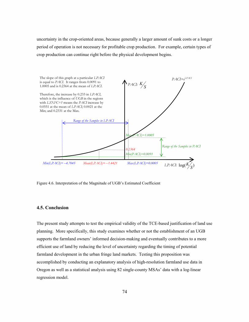
74

PACI: S

K

Max(PACI)=1.0005

LPACI: )log(S

K

Min(PACI)=0.0091

Min(LPACI)= –4.7045 Max(LPACI)=0.0005 Mean(LPACI)= –1.4421

Range of the Samples in LPACI

Range of the Samples in PACI

PACI=eLPACI

0.2364

The slope of this graph at a particular LPACI is equal to PACI. It ranges from 0.0091 to 1.0005 and is 0.2364 at the mean of LPACI. Therefore, the increase by 0.233 in LPACI, which is the influence of UGB in the regions with LSNFC=1 means the PACI increase by 0.0551 at the mean of LPACI; 0.0021 at the Min; and 0.2331 at the Max.

uncertainty in the crop-oriented areas, because generally a larger amount of sunk costs or a longer

period of operation is not necessary for profitable crop production. For example, certain types of

crop production can continue right before the physical development begins.

Figure 4.6. Interpretation of the Magnitude of UGB’s Estimated Coefficient

4.5. Conclusion

The present study attempts to test the empirical validity of the TCE-based justification of land use

planning. More specifically, this study examines whether or not the establishment of an UGB

supports the farmland owners’ informed decision-making and eventually contributes to a more

efficient use of land by reducing the level of uncertainty regarding the timing of potential

farmland development in the urban fringe land markets. Testing this proposition was

accomplished by conducting an explanatory analysis of high-resolution farmland use data in

Oregon as well as a statistical analysis using 82 single-county MSAs’ data with a log-linear

regression model.

75

Through the exploration of farmland use data in Oregon, the results revealed that:

1) Tree fruits and tree nuts, which generally require a larger amount of sunk costs and a

longer period of operation for the profits, is more likely to be grown outside of UGBs

rather than within UGBs, even if the distance to the cities is controlled. This may

suggest that the farmland owners exploit the information contained in UGB plans in their

decision-making, become more certain about the timing of potential land development,

and enjoy a wider range of item choice options if their land is not included in the growth

boundaries (i.e. information is available that the area will not be developed soon.)

2) Fallow/Idle cropland, which may indicate inactive use of farmland while waiting

development rather than soil quality improvements for a long-term agricultural purpose

in this case, is less likely to appear outside of UGBs, compared to the areas within UGBs.

This may also be evidence of the UGB’s effect on uncertainty reduction, thereby offering

support for the TCE-based arguments. In other words, the UGB establishment informs

many farmland owners (having the areas out of the UGBs) that their parcels are not

going to be developed soon and, consequently, induces a more intensive and efficient use

of land.

According to the MSA-level statistical analysis, regressing available independent variables on log

of per acre capital investment (LPACI),

1) For Population growth rate (PGR), negative estimated coefficients are obtained with a

very high level (0.1%) of statistical significance. This may imply that the farmland

owners’ decision making is indeed a strategic choice looking forward and that the

uncertainty, which could be represented by the variable, exists, as argued by TCE-based

justification of land use planning practice.

2) For the variable indicating the Presence of an UGB (UGB), positive coefficients were

found that suggest that the UGB establishment reduces the uncertainty and further

facilitates capital investment for agricultural production. However, the estimated

coefficient is statistically significant (5%-level), only in the MSAs having relatively

larger shares of livestock and fruit production, as opposed to crops; these activities

generally require a greater amount of sunk costs as well as a longer operation period to

be profitable. The insignificance of the estimates for other MSAs may need to be

76

explained by the weak connection between the uncertainty and capital investment, rather

than no or weaker UGB’s effect on uncertainty reduction.

Overall, this study empirically validates the TCE-based justification of land use planning. It is

suggested that uncertainties exist in land markets and prevent economically efficient use of land.

Furthermore, land use planning practice may help land-owners make better land use-related

decisions by proving the relevant information and reducing the level of uncertainties. In this

sense, governments’ involvement in land use and development may be warranted, because of the

higher efficiency of information production and exchange, beyond the appropriateness of

regulatory actions.

Finally, it should be emphasized that this contribution of land use planning may not be trivial.

The UGB’s effect on agricultural investment estimated in this study (i.e. 22.7 million dollars in

the case of a medium size single-county MSA) may turn out to be a very small portion of the full

potential contribution. Land use planning practice may inform not only the farmland owners in

urban fringe areas but also land developers in this particular situation. More generally, a larger

amount of benefits may arise in urban areas where various kinds of uncertainties along with

dramatic internal changes exist, which in turn causes a greater amount of transaction costs and a

greater demand for the systematic management of land use.

77

5. THE MACROECONOMIC EFFECTS OF REACTIVE SUBURBAN LAND USE

REGULATIONS: A SIMULATION STUDY USING A SPATIAL REIM

5.1. Introduction

As summarized in the literature review, the performance of a regional economy is likely to be

influenced by interventions in land development, which significantly affect its property and labor

markets as well as overall spatial structure. It seems that this issue, namely the macroeconomic

effects of land use regulations, has attracted a great deal of attention by planning academics and

the planning profession as a whole. Recently, even a greater deal of attention is paid to the issue,

as policy makers explore the full vision of sustainable development by reconciling the potential

conflicts among economic, environmental, and social goals (Campbell 1996).

How does a particular type of land use regulation affect a regional economy? How can we better

assess the effects? In thinking about the issue, at least two very important dimensions of the

subject need to be considered. The first one is the complexity and dynamics of regional

economies. Generally, a regional economic system is structured by many sectors and

components that are highly interrelated in multiple markets and also linked through non-market

connections. Therefore, the impact of any event or intervention, including land use regulation, is

inevitably system-wide, even if it is directly related to a part of the system (e.g. housing sector).

Furthermore, the system’s behavior is dynamic, so that a shock presenting one time period often

generates long run consequences. For this reason, it would be desirable to use a simulation model

that better characterizes the structure of a regional economic system and further describes the

dynamic behavior of the system, in order to properly assess the effects of land use regulation on a

regional economy.31

31 A simulation model is an excellent instrument that enables scientists to experiment with a system of interest (see. e.g. Frigg & Hartmann 2006). It is more valuable, especially when the system is very complex and cannot be experimented with in the real world. Despite some disadvantages, such as inherent biasedness of modeler, “Modeling and Simulation” has been appreciated in the field of planning, because 1) it enables us to conduct valuable experiments about urban system under various conditions and to answer many “what if?” questions that we frequently asked in the process of planning practice and 2) it allows us to conduct an analysis with a long time frame, which is essential for planning practice dealing with not only short-term but also long-term future.

78

Secondly, consideration needs to be given to the way in which land use regulations are

implemented. In the U.S. context, land use regulations and public goods provisions are typically

under the control of local authorities rather than region-wide planning agencies, although

metropolitan-level or state-level involvement is not absent. Also, a large degree of heterogeneity

is likely to exist within a region.32 Thus, it is necessary to appropriately deal with the spatial

organization of local decision-making and to consider the interaction between local and region-

wide variables over hierarchy. If a simulation model is adopted because of its methodological

advantages for the analysis, it needs to be designed to handle these spatial and multi-level aspects

of the problem.

In the urban economics literature, there are a series of theoretical studies that analyze the

economic consequences of zoning or growth controls by employing a spatial general equilibrium

framework, in which land use and regional economy are interrelated (see e.g. Brueckner 1990;

Engle 1992; Sakashita 1995; Sasaki 1998; Lai & Yang 2002; Sheppard 2004). These studies

have contributed a great deal to improving our understanding of the economic effects of land use

regulation. However, the complexity and dynamics of the problem are too often simplified in

most of these theoretical studies, so their framework, as it stands, has limited usefulness in

simulating the reality. In particular, it is difficult to examine the outcomes of policy options or to

explore for the role of planning practice in complex metropolitan areas.33 For example, many of

the models posit a monocentric spatial structure and single government having the authority of

land use control. Also, the models often lack consideration of detailed industrial structure,

demographics, irregular physical characteristics, and so forth.

Although various operational urban and regional system models have been developed and are

now available for policy and impact analyses, most of them have limited usefulness in analyzing

the effect of local land use policies on regional economic performance, due to the top-down

approach to regional – local integration. In a recent study (Kim & Hewings 2010), an

investigation of the integrated analytic frameworks of 26 large U.S. metropolitan areas’ planning

32 Following Tiebout’s (1956) pioneering examination, a voluminous literature has discussed the variance in local actions (see e.g. Ross & Yinger 1999 for a detailed summary). Also the presence of intraregional heterogeneity has been shown by some empirical studies, such as Heikkila (1996) and McDonald & McMillen (2004). 33 A notable exception is the RELU-Trans model, developed by Anas and his colleagues through their long efforts to integrate regional economy, land use, and transportation within a general equilibrium framework (See e.g. Anas & Kim 1996, Anas & Xu 1999, and Anas & Liu 2007). Their model is considered as one of the most theoretically robust operational urban system models, because of its solid microeconomic foundation.

79

agencies was made and the results revealed that most of them, except Atlanta, Portland, and San

Diego, adopted a strict top down approach to the vertical integration (table 5.1). In these models,

regional variables are typically determined without consideration of local conditions; and then,

the local growth dynamics were strictly bounded by fixed regional totals in most cases. 34

Table 5.1. The Analytic Frameworks of 26 Large U.S. Metropolitan Planning Agencies (As of July 2009)

Representa-tive City

Organization

Regional Growth

Modeling Method

Sub-regional Development Modeling

Method

Approach to Vertical

Integration

Atlanta Atlanta Regional Commission REIM

(REMI) Simulation Model

(PECAS) Feedback

Boston Boston Metropolitan Area Planning Council

Cohort-Component

Share-based Allocation Top-down

Buffalo Greater Buffalo-Niagara Regional Transportation Council

Other Type Share-based Allocation Top-down

Chicago Chicago Metropolitan Agency for Planning

REIM Share-based Allocation Top-down

Cincinnati Ohio-Kentucky-Indiana Regional Council of Governments

External Share-based Allocation Top-down

Cleveland Northeast Ohio Areawide Coordinating Agency

External Share-based Allocation Top-down

Columbus Mid-Ohio Regional Planning Commission

External Share-based Allocation Top-down

Dallas North Central Texas Council of Governments

External Simulation Model (DRAM/EMPAL)

Top-down

Detroit Southeast Michigan Council of Governments

REIM (REMI)

Simulation Model (UrbanSIM)

Top-down

Houston Houston Galveston Area Council Other Type Simulation Model

(UrbanSIM) Top-down

Kansas City Mid-America Regional Council REIM

(REMI) Simulation Model (DRAM/EMPAL)

Top-down

Los Angeles Southern California Association of Governments

Cohort-Component

Other Type Top-Down

Milwaukee Southeastern Wisconsin Regional Planning Commission

Cohort-Component

Other Type Top-down

34 This does not imply that regional as well as local projections used for planning practices are not under local reviews. Rather, this indicates that in the analytic frameworks, the sum of all local-level values is strictly controlled by the regional totals, while regional variables are independent of the local indicators. Although the outcomes of the models, particularly socio-economic forecasts, are the subject of local reviews to some extent before approval, such review processes are generally an adjustment of model outcomes rather than a modification of model structure or formulation. In many metropolitan planning agencies, local level variables are determined by using a share-based allocation approach where attention is paid to the share only, accepting the given totals to be multiplied. The top-down approach is also adopted by the agencies, employing various urban system simulation models for their sub-regional level analysis. This may be attributed to the designs of the simulation models, where regional totals, as exogenous inputs, are required. Under this setting, sub-regional analyses are nothing other than the allocation procedure of regionally-determined growth, so that here the region-wide growth is not influenced by local actions, including land use regulations.

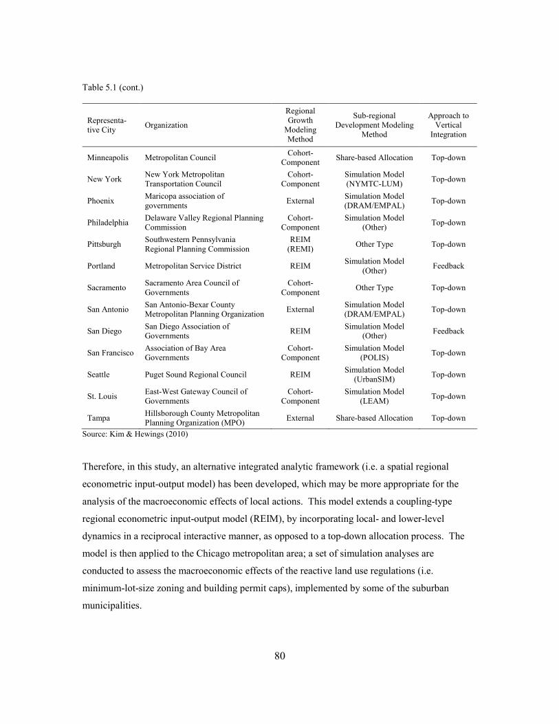
80

Table 5.1 (cont.)

Representa-tive City

Organization

Regional Growth

Modeling Method

Sub-regional Development Modeling

Method

Approach to Vertical

Integration

Minneapolis Metropolitan Council Cohort-

Component Share-based Allocation Top-down

New York New York Metropolitan Transportation Council

Cohort-Component

Simulation Model (NYMTC-LUM)

Top-down

Phoenix Maricopa association of governments

External Simulation Model (DRAM/EMPAL)

Top-down

Philadelphia Delaware Valley Regional Planning Commission

Cohort-Component

Simulation Model (Other)

Top-down

Pittsburgh Southwestern Pennsylvania Regional Planning Commission

REIM (REMI)

Other Type Top-down

Portland Metropolitan Service District REIM Simulation Model

(Other) Feedback

Sacramento Sacramento Area Council of Governments

Cohort-Component

Other Type Top-down

San Antonio San Antonio-Bexar County Metropolitan Planning Organization

External Simulation Model (DRAM/EMPAL)

Top-down

San Diego San Diego Association of Governments

REIM Simulation Model

(Other) Feedback

San Francisco Association of Bay Area Governments

Cohort-Component

Simulation Model (POLIS)

Top-down

Seattle Puget Sound Regional Council REIM Simulation Model

(UrbanSIM) Top-down

St. Louis East-West Gateway Council of Governments

Cohort-Component

Simulation Model (LEAM)

Top-down

Tampa Hillsborough County Metropolitan Planning Organization (MPO)

External Share-based Allocation Top-down

Source: Kim & Hewings (2010)

Therefore, in this study, an alternative integrated analytic framework (i.e. a spatial regional

econometric input-output model) has been developed, which may be more appropriate for the

analysis of the macroeconomic effects of local actions. This model extends a coupling-type

regional econometric input-output model (REIM), by incorporating local- and lower-level

dynamics in a reciprocal interactive manner, as opposed to a top-down allocation process. The

model is then applied to the Chicago metropolitan area; a set of simulation analyses are

conducted to assess the macroeconomic effects of the reactive land use regulations (i.e.

minimum-lot-size zoning and building permit caps), implemented by some of the suburban

municipalities.

81

The remainder of this paper is structured as follows. Section 5.2 first provides a concise

explanation of a REIM, which is the starting point of the spatial REIM development. Then, the

discussion turns to the way in which the spatial REIM has been constructed on the REIM with an

emphasis on the ways in which local variables are incorporated and vertical interaction is handled.

In section 5.3, the model is applied to the Chicago metropolitan area and the baseline projections

for individual municipalities as well as the Chicago region as a whole are generated. The

simulation analyses are presented in section 5.4, followed by a summary and discussion.

5.2. Modeling: A Spatial REIM

5.2.1. Conventional REIM

This study develops an alternative framework that overcomes the shortcomings of existing

models and can be used for the analysis of the macroeconomic effects of local actions,

particularly land use regulations. Before presenting the new framework, in this section, a concise

explanation will be provided of the conventional regional econometric input-output models

(REIMs), particularly the Chicago REIM (Israilevich et al. 1997), on which the new framework is

built.

By integrating regional input-output (hereafter IO) and econometric, the REIMs exploit the

advantages of both methods. In fact, this ‘IO+econometric’ integration offers the possibility of

making the regional IO matrix dynamic and price-responsive and to forecast the growth, decline,

and transformation of the regional economy with the consideration of a disaggregated industrial

structure (see e.g. West & Jackson 1998; Rey 2000).

More specifically, the Chicago REIM (CREIM), here a basis for the new integrated framework

development, is a coupling-type REIM (according to Rey’s (1998) taxonomy) for the Chicago

region. Its structure, most simply, can be demonstrated in figure 5.1.

82

Figure 5.1. Conventional CREIM Structure

The CREIM’s logic starts from the exogenous national economy (and implicitly, the international

economy), driving or constraining Chicago’s economic growth, as a major source of demand for

regional production. As the national economy grows, Chicago’s production is stimulated; this

initial stimulus generates not only the immediate production increase but also ripple effects

through regional inter-industry linkages. This mechanism is simulated by CREIM’s dynamic

input-output module, which is one of the most important features of CREIM.

The module is designed to consider the dynamic nature of inter-industry and final demand

linkages and to update the IO coefficients over time. Adopting the idea presented in Conway

(1990), here, the temporal IO coefficient changes are described by using two types of output that

interact with each other, rather than a rule or function of direct transformation. More specifically,

consideration is given to two different types of output – 1) “actual output” (X): the real values of

production and 2) “expected output” (Z): the expected level of outputs, derived from the base

year’s input-output matrix. By definition, these two variables are related to each other, as follows.

FXAZ +⋅= (5-1)

where A is a base year’s input-output matrix and F represent final demands.

Dynamic IO: Actual Output (X) – Expected Output (Z) Interaction

Employment(E)

Income (Y)

Population (P)

Final Demand(F)Output

National Economy

83

In base year, Z is exactly same as X ( i.e. XFXAZ =+⋅= ), because A is the IO for that year.

Also, if the IO coefficients (A) were not changing over time, the equation Z=X can be maintained

in all other years. In reality, due to the technological shifts and other factors affecting the

production recipe changes, IO coefficients are not constant but evolving over time. Consequently,

Z and X are rarely identical, although they are associated with each other.

Figures 5.2 and 5.3 show Z and X in two sectors as examples – 1) Sector 18: Fabricated metal

products manufacturing and 2) Sector 35: Real Estate.35

Z & X: Sector18 Fabricated Metal Products

0

5,000

10,000

15,000

20,000

25,000

1969

1970

1971

1972

1973

1974

1975

1976

1977

1978

1979

1980

1981

1982

1983

1984

1985

1986

1987

1988

1989

1990

1991

1992

1993

1994

1995

1996

1997

1998

1999

2000

2001

2002

2003

2004

2005

Year

Value (2005 Chained Million$)

Z18 X18

Figure 5.2. Expected Output (Z) and Actual Output (X) in Fabricated Metal Products Manufacturing (1969~2005)

35 The data series Z can be generated by using historical data of actual output (X) by sector and final demands (F) as well as a base year IO matrix (A).

84

Z & X: Sector35 Real Estate

0

10,000

20,000

30,000

40,000

50,000

60,000

1969

1970

1971

1972

1973

1974

1975

1976

1977

1978

1979

1980

1981

1982

1983

1984

1985

1986

1987

1988

1989

1990

1991

1992

1993

1994

1995

1996

1997

1998

1999

2000

2001

2002

2003

2004

2005

Year

Value (2005 Chained Million$)

Z35 X35

Figure 5.3. Expected Output (Z) and Actual Output (X) in Real Estate (1969~2005)

Here, the base year is Year 2005, where Z and X are identical. In all other years, Z is not equal to

X; and sometimes they reveal large differences. More specifically, in the case of Sector 18:

Fabricated metal products manufacturing, X is much greater than Z in 1970s and 1980s, while the

gaps are relatively smaller since 1990 (figure 5.2). This implies that the level of output will be

underestimated, if the base year IO table is used for 1970s and 1980s. In other words, the current

linkages of this industry to other sectors in the Chicago economy are weaker than those in past

(i.e. 1970s and 1980s). This is consistent with the understanding of changes in the Chicago

economy, particularly the increased locational fragmentation of manufacturing activities

(implying declining forward and backward linkages) in that period of time (see Hewings et al.

1998, Okuyama et al. 2002 and 2006). The real estate sector, which is primarily local, shows a

different trajectory of Z and X over time, with little evidence of fragmentation, unlike

manufacturing (figure 5.3).

Finally, Z and X need to be related econometrically. In the process, a dynamic IO, which is

embedded in the model, will be generated; further, it will be possible to obtain actual output (X)

in the future corresponding to the final demands (F) and the updated IO. In CREIM, this is

accomplished in the following form.

85

titig

ti

ti

Z

ti

tig

z

x

z

x,,

1,

1,

0

,

,)ln( εααα +⋅+

⋅+=

−

− (5-2)

where i and t are industry and time subscripts, respectively; and g represent a set of exogenous

variables. It needs to be noted that the lag structure (e.g., first order or second order) varies by

sector depending on the fitness. As demonstrated in Israilevich et al. (1996), this specification

captures the lag effect of any shock in IO coefficients.

Once the output (X) is derived based on the dynamically updated IO module in the model,

employment (E) by industry needs to be projected. This can be accomplished by forecasting

regional labor productivity using national productivity projections, which are exogenous, as

shown below.

ti

ti

tif

e

x,

,

,)()ln( φ+⋅= →

])(exp[ ,

,

,

ti

ti

tif

xe

φ+⋅= (5-3)

where f(·) is industry-specific regional productivity function; and ti,φ is an error term.

Then, based on the employment projection, CREIM generates income (y) by sector in a similar

manner.

ti

ti

tih

e

y,

,

,)()ln( ω+⋅= → ])(exp[ ,,, tititi hey ω+⋅⋅= (5-4)

where h(·) is industry-specific regional wage function; and ti ,ω is an error term. In this case, the

national wage level is used as the main exogenous independent variable.

As income is derived from employment, CREIM sets working age population as a function of

regional employment as well as other factors. In addition, regarding population, birth and death

rates in future are forecast primarily based on historical trends, and also applied to generate the

projections for population by cohort. Net migration is also estimated, completing the

demographic accounting.

Then, using both income and population, the endogenous final demand levels – i.e. various types

of consumption, investment, and state and local government spending – are determined. Finally,

86

the model is brought to closure by linking the endogenously determined final demands back to

the input-output module, particularly F in equation (5-1): FXAZ +⋅= .

The regional economic and population forecasts can be generated, once the entire model is

constructed, through the estimation of all equations in the input-output module as well as

employment, income, population and final demand bloc. Forecasting identifies the solutions for

the entire set of equations and identities for every forecast year. In this sense, it can be stated that

the forecasts represent a sort of general equilibrium state where all markets are balanced. That is

the reason why this type of REIM is sometimes referred to as a Marshallian type of general

equilibrium model in which commodity adjustments (through changes in the IO coefficients)

facilitate market equilibrium at each point in time.

It needs to be emphasized that, although not perfect, the model systematically connects various

macroeconomic variables; and it is designed to describe the dynamic behaviors of the system.

Particularly, detailed inter-industrial linkages are well characterized in a dynamic manner. Also,

the model integrates regional population and employment in a reciprocal manner. One the one

hand, as mentioned above, regional employment is used to explain changes in working age

population. On the other hand, population is linked to the regional economic production (X) via

final demands (i.e. household consumption and expenditure of state and local governments); and

further employment (E), which is derived from the production, creating an endogenous multiplier

process.

5.2.2. Spatial REIM: A Multi-level Integrated Analytic Framework

The REIMs are relatively more sophisticated regional macro-economic tools which support

regional economic forecasting and economic impact analysis based on dynamically updated IO.

This family of the models has been widely employed by applied research since 1980s and has

now become a key analytic tool, competing with Walrasian computable general equilibrium

models (see e.g. West 1995; Rey 2000). According to Kim & Hewings (2010), this technology is

increasingly adopted by metropolitan planning agencies as well to generate region-wide forecasts

and to conduct the analysis of regional economic scenarios.

87

However, the conventional REIMs (including CREIM), as they stand, only focus on the

macroeconomic and region-wide demographic behaviors.36 The models neither support

disaggregated-level analysis or forecasting nor consider the sub-regional-level conditions or the

spatial structure of the region.37 In order to overcome this limitation and further to make a multi-

level framework which is suitable for the analysis of land use regulations, the REIM (particularly

CREIM) will now be developed into a spatial REIM where 1) attention is also paid to the

dynamics within a region and 2) regional- and sub-regional variables are vertically integrated in a

reciprocal interactive form.

The proposed new framework has a hierarchical structure (as opposed to the REIM having

region-wide variables only) that consists of 1) three endogenous layers: region – municipalities –

cell and 2) national economy as an exogenous input remains on the top. Rather than simply

allocating the region-wide totals generated by the conventional REIMs, here the main idea of the

framework development is to establish a reciprocal vertical integration (figure 5.4) – i.e. in every

round of model run (i.e. in each year (t) of the projection) the model is working across the

hierarchy as follows:

1) Using national economic forecasts for year t, the potential (expected) regional

economic growth rate by sector is first derived from the regional layer.

2) The cell-level information (i.e. lowest level conditions) at t-1 for each municipality

is quantified to be taken into account in local level forecasting and analysis at t.

3) Local level population and employment changes are tentatively determined with the

consideration of a) the region-wide potential growth at t, b) the cell-level conditions

at t-1, c) local socio-economic characteristics at t-1, and d) local level ‘population –

employment’ interactions across space.

4) The tentative values of local population and employment changes are sent back to

the regional-level to project macro-economic variables, which are systemically

integrated with each other according to the REIM formulation.

36 There have been the extensions of the conventional REIMs, such as the application to multi-regional contexts or the temporal disaggregation (see e.g. Rey & Dev. 1997; Donaghy et al. 2007). However, the incorporation of intraregional dynamics (i.e. development of the spatial REIM) has not been accomplished. 37 Therefore, when this modeling technology is adopted by metropolitan planning agencies, it is used only for generating regional level forecasts or region-wide impact analysis; and sub-regional level values are separately determined by using share-based allocation techniques or urban simulation models that just allocate the given totals (from REIMs) across space within the region (Kim & Hewings 2010). Again, the combined use of a REIM and a disaggregation tool has been typically made in a top-down manner.

88

*) Then, the potential (expected) growth rate by sector is newly derived based on the

new levels of final demands. (1) – (3) – (4) processes are iterated until convergence,

with given (2).

5) Once the values of all regional and local variables for year t are finally determined

through the iteration, cell level conditions are updated from t-1 to t by employing a

simple logic or a more sophisticated simulation method. The updated cell-level

information is used in the next round (i.e. year t+1).

Figure 5.4. The Spatial REIM Structure, as Opposed to a Traditional REIM & Allocation

Employment Income

Population

Final DemandOutput

National Economy

Sub-regionalEmployment

More disaggregated level variables(e.g. Land use by parcel)

Sub-regional

Population

Employment Income

Population

Final DemandOutput

National Economy

Cell- (or Parcel-)

level Variables

Local-level

Employment

Local-level

Population

PotentialEmployment Growth

Dynamic IO Dynamic IO

Traditional REIM & Allocation: Top-down A Spatial REIM Structure

①

①

② ②

③

⑤ ⑤

④ ④

89

The third step is the most important part of this model formulation and operation. Although

various methods can be adopted for this stage, use here is made of a spatial econometric version

of regional disequilibrium adjustment model (RDAM), that has a following spatial cross-

regressive simultaneous equation system (according to Rey & Boarnet’s (2004) taxonomy), as

explained in detail in section 3.3.1.

ti

k

tp

k

t

E

Pp

k

tPpPp

k

t

k

t

uPEWI

EWIHP

,)(

)(

+⋅−∆⋅+⋅⋅

+

⋅+⋅⋅+⋅⋅=∆

λλ

θλ

θλβλ

(5-5)

ti

k

tE

k

t

P

EE

k

tEEEE

k

t

k

t

vEPWI

PWIBE

,)(

)(

+⋅−∆⋅+⋅⋅

+

⋅+⋅⋅+⋅⋅=∆

λλθλ

θλβλ (5-6)

where k and t denote cross sectional unit (e.g. municipalities) and time, respectively.

The RDAM’s dynamic nature and explicit treatment of disaggregated-level population and

employment changes together with the consideration of their spatial interdependence promote its

use combined with a REIM. In addition, the benefits of using a RDAM could be larger than

expected, since many local or lower level factors, such as social indicators, land use, and

location-specific amenities, can be conveniently included as exploratory variables to determine

local population and employment changes.

However, because it primarily focuses on population and employment changes originating from

the spatial adjustment process and intraregional location factor differentials, a RDAM itself is not

suitable for long-term forecasting, even though the dependent variables are population and

employment changes. To be an effective supporting tool for long-term analysis, the system

would need to consider the fundamental growth drivers. This is the reason why the potential

(expected) growth is derived in step (1) and used in local forecasting and analysis.38

38 It needs to be emphasized that the forecasting accuracy can be improved by the inclusion of upper-level estimates in the model for disaggregated-level variables. Zellner & Tobias (2000) compared seven models which can be classified into three main categories – 1) aggregated-level forecast, 2) disaggregated-level forecast, and 3) using the aggregated-level forecasts in disaggregated-level forecasting as an explanatory variable – and found that the third approach shows the best performance.

90

More specifically, instead of the actual employment change between t-1 and t (i.e. k

tE∆ ), the

dependent variable of the employment change equation is set as below.

k

t

k

t

k

t

k

t

k

t

k

t

k

t

k

t

k

t ZEEEZEEEEZEE −=−−−=−−∆ −−− )()()( 111

where k

tZE is the potential level of employment, calculated based on the region-wide potential

employment growth rate by sector between t-1 and t.

This new dependent variable indicates the number of job increase beyond the potential (expected)

level of growth. If a particular municipality shows actual employment growth larger than

expected for a certain time period, the value of the variable will be positive. In contrast, if it fails

to attain the expected level of growth, the value will become negative.

k

tZE is computed as follows (Step 1 in the model working). First of all, the potential regional-

level employment growth rate by sector is derived using the concept of expected output (Z),

existing in CREIM.

1,

,

1,

1,

0,

1,

,

)(exp

−

−

−

−

⋅−⋅+

⋅+⋅

=ti

tig

ti

ti

Zti

ti

ti

e

fgz

xz

e

zeααα

(5-7)

where tize , is the expected level of regional employment in sector i at time t; and the multiplied

part in the form of exp( ) is industry-specific function which converts Z to employment via X, as

presented in equation (2) and (3). The numerator of this equation indicates the number of

employees that the producers in sector i may hire to meet demand growth. Whereas the

numerator is adopted as the predicted value of employment in sector i at time t in the

conventional CREIM without consideration of local conditions or supply constraints, the new

framework uses it as an indicator that represents the potential employment growth of each

municipality, as further explained below.

Then, this expected rate of employment growth by sector is applied to individual municipality’s

employment at time t-1(k

tie 1, − ) to generate the expected employment level at time t in

municipality k (i.e. k

tZE ), as follows:

91

1,

,

1,,

−− ⋅=

ti

tik

ti

k

tie

zeeze (5-8)

∑=i

k

ti

k

t zeZE , (5-9)

This expected employment level of each municipality can be understood as the sum of growth

and industry-mix effect in the context of shift share analysis, although the “expected” change by

sector in a higher-level, as opposed to the “actual” change, is used. In this sense, the new

dependent variable, which is the residual (i.e. k

t

k

t ZEE − ), represents the competitiveness of each

municipality in terms of job attraction. In other words, given that the new dependent variable is

adopted, the employment change equation tries to capture the variance of the competitiveness

across municipalities by using the changing proximity to population and other business location

factors. This is a feature in various urban system simulation models, ranging from Lowry-type

spatial interaction frameworks to micro-simulation and spatial IO approaches (see e.g. Wegner

1994; Hunt et al. 2005; Kim & Hewings 2010)

In a similar way, the population change equation is modified. Here, the new dependent variable,

used instead of k

tP∆ , is

k

t

k

t

k

t

k

t

k

t

k

t

k

t

k

t

k

t ZPPPZPPPPZPP −=−−−=−−∆ −−− )()()( 111

where k

tZP is the potential (expected) level of population, which is simply computed by

multiplying the natural population growth rate (i.e. the gap between the birth rate and death rate)

and k

tP 1− .

In the present application of the spatial REIM, for simplicity and due to the data availability

problem, the birth rate and death rate are exogenously determined using regional level

information; and no consideration is given to the different rates for different cohort groups.

However, the demographics can be further extended by introducing the logic of the cohort

component survival model as well as exploiting the possibility of using more (spatially) detailed

migration data.

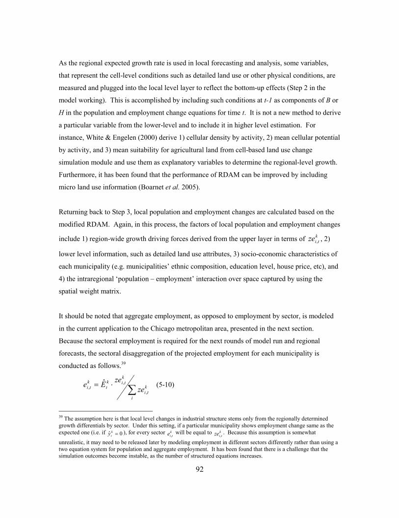
92

As the regional expected growth rate is used in local forecasting and analysis, some variables,

that represent the cell-level conditions such as detailed land use or other physical conditions, are

measured and plugged into the local level layer to reflect the bottom-up effects (Step 2 in the

model working). This is accomplished by including such conditions at t-1 as components of B or

H in the population and employment change equations for time t. It is not a new method to derive

a particular variable from the lower-level and to include it in higher level estimation. For

instance, White & Engelen (2000) derive 1) cellular density by activity, 2) mean cellular potential

by activity, and 3) mean suitability for agricultural land from cell-based land use change

simulation module and use them as explanatory variables to determine the regional-level growth.

Furthermore, it has been found that the performance of RDAM can be improved by including

micro land use information (Boarnet et al. 2005).

Returning back to Step 3, local population and employment changes are calculated based on the

modified RDAM. Again, in this process, the factors of local population and employment changes

include 1) region-wide growth driving forces derived from the upper layer in terms of k

tize , , 2)

lower level information, such as detailed land use attributes, 3) socio-economic characteristics of

each municipality (e.g. municipalities’ ethnic composition, education level, house price, etc), and

4) the intraregional ‘population – employment’ interaction over space captured by using the

spatial weight matrix.

It should be noted that aggregate employment, as opposed to employment by sector, is modeled

in the current application to the Chicago metropolitan area, presented in the next section.

Because the sectoral employment is required for the next rounds of model run and regional

forecasts, the sectoral disaggregation of the projected employment for each municipality is

conducted as follows.39

∑

⋅=

i

k

ti

k

tik

t

k

ti ze

zeEe

,

,,

ˆ (5-10)

39 The assumption here is that local level changes in industrial structure stems only from the regionally determined growth differentials by sector. Under this setting, if a particular municipality shows employment change same as the

expected one (i.e. if 0ˆ =k

ty ), for every sector k

tie , will be equal to k

tize ,. Because this assumption is somewhat

unrealistic, it may need to be released later by modeling employment in different sectors differently rather than using a two equation system for population and aggregate employment. It has been found that there is a challenge that the simulation outcomes become instable, as the number of structured equations increases.

93

Here, k

tE is the projected employment for municipality k, that is equal to k

t

k

t ZEy +ˆ , where k

ty

is the predicted value of the modified RDAM employment equation.

As mentioned above, the calculated values of local population and employment for t are sent back

up to regional-level layer to project macro-economic variables (Step 4 in the model working). In

detail, first region-wide population and sectoral employment are calculated by summing up the

employment and population of all municipalities.40 Then, all other macroeconomic variables are

determined according to the REIM formulation.41 Further, the expected output (Z) will be newly

calculated using the new final demands as well as the actual output (X), based on the equation (5-

1): FXAZ +⋅= .

The newly calculated Z generates a new series of the potential level of employment for individual

municipalities (k

tZE ). In other words, step 1 of the modeling working is repeated. (Step 1) –

(Step 3) – (Step 4) processes need to be iterated until convergence to finally determine local

population and employment as well as regional variables for t.

Once this is done, cell level conditions need to be updated from t-1 to t based on the new local

population and employment (Step 5). For instance, to be consistent with the determined

population and employment increases between t-1 and t, an appropriate number of undeveloped

cells within a municipality need to be converted to residential and commercial-industrial land

uses respectively. This task can be accomplished by simple updating or through the use of a more

sophisticated simulation method. The updated cell-level information is again plugged into the

local level layer as explanatory variables in the population and employment change equations for

time t+1. This is for step 2 of the model flow-chart in the next round.

Suppose that a key sector of the study region is projected to grow very rapidly, according to the

national economic forecasts. Under these national economic forecasts, the REIM tends to

generate a rapid increase in regional employment in many others as well as the sector. If we

40 In real applications, regional and local level may have different levels of sectoral details, because of data availability (i.e. generally, much disaggregated information is only available for regions.) If this is the case, appropriate aggregation and disaggregation process is required when the values are transferred over hierarchy. 41 While the actual output (X) is generated by the equation (2) using Z in the conventional REIM, it is now derived by the equation (3) using the locally determined employment level.

94

adopt the conventional CREIM, a large employment growth will be placed in the region

regardless of local conditions. In contrast, the spatial REIM framework transmits this signal to

the local level, particularly to the municipalities having greater numbers of employment in the

key sector and checks whether or not the rapid demand increase of this sector’s employment can

be satisfied by the existing local and lower level conditions, so that a large amount of multiplier

effects can be realized. If many establishments in this sector are currently located in a very

congested zone where growth cannot be accommodated efficiently, the level of actual

employment growth in the sector may be projected to be lower than the expected level at the local

layer; and the regional employment growth trajectory is also altered according to the modified

employment increase.42 This may be more consistent with the reality that the chance of attaining

the potential growth in the region is influenced by the internal conditions.

This is what the spatial REIM attempts to describe by establishing a feedback link that was

described earlier. More generally, it tries to reflect the probable supply constraints and the effect

of regional spatial structure on the performance of a regional economy, rather than assuming that

all demand increases will be satisfied and that the additional activities to meet the demand

increase will be located somewhere within the region.

5.3. An Application of the Spatial REIM: The Case of Chicago

5.3.1. Study Area

The established framework is applied to the Chicago metropolitan area by extending the 2008

version of CREIM (Base year: Year 2005). In this version of CREIM, the economy of the seven-

county Chicago Metropolitan Agency for Planning (CMAP) region – Cook, DuPage, Kane,

Kendall, Lake, McHenry, and Will in Illinois – is described with a new industrial classification

system that consists of 45 NAICS-based industries and government sectors, listed in table 5.2.

The 2008 CREIM, estimated with historical data between 1969 and 2005, is capable of producing

42 One critical issue in modifying the regional growth trajectory may be whether the unmet potential growth will be deflected to another part of the metropolitan area or outside the region. The spatial REIM does not directly describe this behavior of the system. Rather, in the model, the modified trajectory is determined by solving the entire set of macroeconomic and the RDAM equations under given conditions through the iteration.

95

the macroeconomic forecasts from 2006 up to 2040 by using national economic forecasts for the

corresponding forecast years.

Figure 5.5. Study Area: Seven County CMAP Region

Table 5.2. Industry Classification System of CREIM

Code Description 2002NAICS

01 Livestock and Other Agricultural Products 111, 112

02 Agriculture, Forestry and Fisheries 113, 114, 115

03 Mining 21

04 Utilities 22

05 Construction 23

06 Food and Kindred Products 311

07 Tobacco Product Manufacturing 312

08 Apparel and Textile Products 313, 314, 315

09 Leather and Leather Products 316

10 Lumber and Wood Products 321

11 Paper and Allied Products 322

12 Printing and Publishing 323, 511, 516

Lake Michigan

Chicago

96

Table 5.2 (cont.)

Code Description 2002NAICS

13 Petroleum and Coal Products 324

14 Chemicals and Allied Products 325

15 Rubber and Misc. Plastics Products 326

16 Stone, Clay, and Glass Products 327

17 Primary Metals Industries 331

18 Fabricated Metal Products 332

19 Industrial Machinery and Equipment 333

20 Computer and other Electric product, component manufacturing 334, 335

21 Transportation Equipment Manufacturing 336

22 Furniture and Related Product Manufacturing 337

23 Miscellaneous Manufacturing 339

24 Wholesale Trade 42

25 Retail Trade 44, 45

26 Air Transportation 481

27 Railroad Transportation and Transportation Services 482, 492, 487, 488

28 Water Transportation 483

29 Truck Transportation, Warehousing, Waste & Remediation services 484, 493, 562

30 Transit and Ground Passenger Transportation 485

31 Pipeline Transportation 486

32 Information, except Motion Picture and Sound Recording Industries 515, 517

33 Motion Picture and Sound Recording Industries 512

34 Finance and Insurance 52, 55, 533

35 Real Estate 531

36 Professional and Management services and other support services 54, 518, 561

37 Educational Services 61

38 Health Care 621, 622, 623

39 Social Assistance 624

40 Arts, Entertainment, and Recreation 711, 713

41 Accommodation Services 721

42 Food Services 722

43 Repair and Maintenance 811

44 Personal and Laundry Services 812

45 Memberships Organizations and Private Households 712, 813, 814

FGE Federal Government Enterprises N/A

OFGC Other Federal Government, Civilian N/A

FGM Federal Government, Military N/A

SLGE State and Local Government Enterprises N/A

OSLG Other State and Local Government N/A

97

There are 296 municipalities within this area, as shown in figure 5.5. While most of them are

completely included in the study area, a few municipalities are located across the region’s

boundaries. The partly included municipalities are considered, with their shares of population

and employment within the portions included in the study area. The unincorporated areas of each

county are considered as a municipality to maintain the identity between the regional values and

the sum of all local units. As a result, there are 303 units of local analysis.

5.3.2. Model Calibration

The main tasks of this spatial REIM application are 1) to calibrate the model by estimating the

modified RDAM, 2) to solve the entire set of equations with a feedback loop for every forecast

year and 3) to generate a set of baseline simulation outcomes. First, for the calibration task, data

for five time spans were used, from [2000,2001] to [2004,2005] due to the data availability

problem. Particularly, there is no single source of information, providing annual employment by

municipality, which is the main variable of this analysis. Therefore, an employment dataset was

constructed using three data sources: 1) 2000 Census Transportation Planning Package (CTPP)

data, 2) Zipcode Business Pattern (ZBP) data by U.S. Census, and 3) Regional Economic

Information System (REIS) data by U.S. Bureau of Economic Analysis. More specifically,

employment by sector in 2000 for individual municipalities was identified using CTPP data that

provides employment information for each census tract in decennial years.43 Then, using the ZBP

dataset, that contains annual establishment and employment information at zip-code area level,

the rate of employment changes from 2000 to other years for each zip-code areas are derived. A

series of spatial smoothing is applied to generate a more realistic surface of employment change

rates across the space. Then, by multiplying the values of smoothed employment change rates

with 2000 employment derived from CTPP, employment by municipality is derived for every

year from 2001 to 2005. Finally, the outcome of the former procedure is adjusted to match to the

values provided by REIS (annual employment by sector at county level), when they are

aggregated up to county-level, because REIS has been used as a main source of information for

CREIM development. Since there are some discrepancies in definitions of employment in

43 Local employment information available is disaggregated by 14 sectors based on NAICS, whereas CREIM has a 45-sector classification scheme. For this reason, aggregation and disaggregation work is conducted when the values are

transferred over hierarchy. It needs to be noted that the potential (expected) employment growth (i.e. k

tize ,) for each

municipality is computed based on the 14-sector classification.

98

different datasets, the gaps to be adjusted are inevitable. A similar approach (i.e. using multiple

data sources and trying to mitigate the discrepancies and errors) is used to cope with the data

availability problems of other variables. The variables used in this analysis and data sources are

presented in table 5.3.

Table 5.3. Variables and Data Sources in the RDAM Estimation

Variable Description Data Sources

Main Variables

P Population Annual Population Estimates by US Census

E Employment CTPP, ZBP and REIS

Derived from Regional level

ZE Expected level of employment3 CREIM

Municipality-level Socio Economic Characteristics

NWR The Ratio of Non-White Population Census 2000 and American Community Survey

HISPR The Ratio of Hispanic Population Census 2000 and American Community Survey

VACR Vacancy Rate Census 2000 and American Community Survey

EDU1 The Level of the Educational Attainment Census 2000 and American Community Survey

MHOHINC Median Household Income Census 2000 and American Community Survey

MHV Median Value of Specified Housing Units Census 2000 and American Community Survey

POVR Poverty Rate Census 2000 and American Community Survey

Micro-level Information

HINTERLA2 The Area of Lands for Potential Incorporation

TIGER4

LU_UDL The Area of Developable Land within the Jurisdictional Boundaries

National Land Cover Database by USGS and CMAP’s Land-Use Inventory

OS The Area of Developed Open Space National Land Cover Database by USGS and CMAP’s Land-Use Inventory

RC The Lengths of the Major Arterial Roads TIGER and Annual road mileage data by Illinois Department of Transportation

GOV Presence of Major Government Offices CMAP’s Land-Use Inventory

UNIV Presence of Universities or Colleges CMAP’s Land-Use Inventory

BIZPARK Presence of Business Parks CMAP’s Land-Use Inventory

DISTCBD Distance to CBD GIS data by City of Chicago

DISTOHARE Distance to O’Hare International Airport GIS data by City of Chicago

1) EDU is defined as a percentage of 25+ population, whose educational attainment is Bachelor's degree or above 2) This is a measurement to consider the area of available hinterlands surrounding each municipality. This represents the area of unincorporated land closet to each municipality. 3) See the equation (5-7)~(5-9) for details. 4) TIGER indicates the Topologically Integrated Geographic Encoding and Referencing system provided by U.S. Census.

99

To complete this RDAM estimation, a spatial weight matrix (W) is necessary. The matrix was

constructed using 2000 municipality-level journey to work data contained in CTPP. This way of

constructing the weight matrix is theoretically desirable, because here the matrix is introduced to

consider the labor market areas beyond municipality boundaries. Also, according to the

experiment by Boarnet et al. (2005), a journey-to-work-data-based weight matrix is more likely

to generate reasonable estimation outcomes.

It should be noted that I make a following treatment on many explanatory variables and use the

converted index value (i.e. index(x)k), as opposed to the real magnitude (xk), in the estimation for

a long-run simulation purpose.

t

t

k

tk

tx

xxxIndex

)(

)()(

σ−

= (5-11)

This treatment may be necessary for the situations such as the following case. Suppose that a

positive and statistically significant effect of HISPR (the ratio of Hispanic population) on local

population change is found with given data. This may be probable, because the newly

immigrated Hispanic population may tend to settle down in the communities where many people

in the same ethnic group are living. As the Hispanic population is moving into the region in

increasing numbers over time, the level of HISPR in most municipalities will increase. If the

population change equation is set as a function of the real magnitude of HISPR with a positive

coefficient, the overall population will be growing rapidly simply because of the generally

increasing HISPR in the region. Although this may be the case in the sense that the Chicago has

come to attract more Hispanic immigrants in competition with other regions, this is not very

probable. Rather, it would be more reasonable to think that the location choice of a certain

number of Hispanic residents or new immigrants is influenced by relative level of HISPR and to

use local HISPR variance within the region to capture this effect. The index, which indicates the

relative position of each municipality on a variable’s distribution, is used for this reason. By

adopting this strategy, the overall increase or decrease in the real magnitude of the variables will

affect the region-wide totals in a more realistic fashion.

Because the modified RDAM is also a spatial cross-regressive simultaneous equation system

having the feedback and spatial simultaneity problems, traditional least square techniques,

including traditional two stage least square, cannot provide consistent and unbiased estimates.

100

Therefore, like the spatial econometric analysis in chapter 3, the model is estimated using a

spatial generalized moments approach, initially developed by Kelejian & Robinson (1993) and

later extended by Kelejian & Prucha (1998 and 1999). More specifically, the simultaneous

equation system model is estimated in a constant coefficients model form. Also, to obtain the

final estimates for the simulation, the model specification is modified repeatedly, by excluding

the independent variables that are statistically insignificant at the 5%-level. Table 5.4 presents

the final estimation outcomes.

Table 5.4. Final Estimation Outcomes of the Modified RDAM

Variable Description Coefficient Standard

Error t-statistic P-value

[Population Change Equation] Dependent Variable: P – ZP

C Intercept 201.061 37.9227 5.30186 [.000]

IWECH (I+W) * (Employment Change) 0.018523 8.14E-03 2.27683 [.023]

P0 Population in t-1 -0.012422 1.26E-04 -98.7758 [.000]

IWE0 (I+W) * (Employment in t-1) 2.74E-04 9.28E-05 2.95723 [.003]

Index(HISPR) HISPR Index 109.496 17.0398 6.42593 [.000]

Index(MHOHINC) MHOHINC Index 101.471 44.0884 2.30155 [.021]

Index(EDU) EDU Index 194.153 31.296 6.20377 [.000]

Index(MHV) MHV Index -276.375 38.7214 -7.13754 [.000]

Index(UNIV) UNIV dummy Index 54.7356 15.5275 3.52507 [.000]

Index(LU_UDL) LU_UDL Index 214.496 18.3866 11.6659 [.000]

Index(HINTERLA) HINTERLA Index 256.229 18.8212 13.6138 [.000]

DUMMYREC1 Dummy of recession years 85.9552 41.4773 2.07234 [.038]

R-squared = 0.884617 | Adjusted R-squared = 0.883772

[Employment Change Equation] Dependent Variable: E – ZE

C Intercept 176.177 44.3415 3.97317 [.000]

IWPCH (I+W) * (Population Change) 0.08044 0.024666 3.26123 [.001]

E0 Employment in t-1 -0.01769 2.43E-04 -72.8692 [.000]

IWP0 (I+W) * (Population in t-1) 5.02E-04 1.58E-04 3.17294 [.002]

Index(HISPR) HISPR Index 116.64 24.0711 4.84565 [.000]

Index(EDU) EDU Index 207.491 40.3936 5.13674 [.000]

Index(MHV) MHV Index -142.785 38.3557 -3.72267 [.000]

Index(GOV) GOV dummy Index 74.2272 22.8953 3.24202 [.001]

R-squared = 0.871904 | Adjusted R-squared = 0.870909

1) In the recession years, while employment decreases significantly, generally net-migration is not much affected in spite of the unfavorable economic situation, because of the similar unfavorable situations in other areas. So, employment is hardly matched to population in a RDAM set-up. By including the dummy variables for such recession years, we can better deal with this unusual mismatch. The dummy variables are expected to exhibit positive coefficients in the population change equation.

101

The overall model’s explanatory power is good (adjusted r-squared are 0.87~0.88). Also, the rate

of adjustment, which are the negative values of the estimated coefficients for P0 in population

change equation (i.e. 0.012422) and that for E0 in employment change equation (i.e. 0.01769),

are between 0 and 1 as expected. This means that the model will generate dynamically stable

processes. Moreover, statistically significant reciprocal ‘population –employment’ interactions

are found (see the estimates for IWECH and IWPCH in the two equations).

In addition, the estimation captures the effects of municipality level socio-economic

characteristics and micro-level attributes on household and business location decisions. For

example, the results revealed that population is more likely to grow in the towns showing higher

ratios of Hispanic population, median income, and education level. The presence of any

university is found to be favorable to population increase, while the relative level of housing price

has a negative effect on population growth. Moreover, large areas of developable or

incorporable land are positive factors of population growth.

In similar fashion to population changes, the estimation outcomes suggest that employment tends

to grow faster than expected if the municipality has a higher Hispanic population ratio or

educational attainment level. In the case of employment, the presence of major government

offices also exhibits a statistically positive effect. However, the presence of business parks and

per capita major arterial road shows statistically insignificant effects.

5.3.3 Model Solving

Using the modified RDAM estimated above, the spatial REIM is constructed according to the

structure presented in the previous section. The overall framework has the equations for the

macro-economic variables in the CREIM and the two equation system for local population and

employment as well as the cell-level module.

The entire set of equations is solved through the five step process for each forecast year, as

explained above. More specifically, once the values of all explanatory variables, including the

potential level of employment for individual municipalities (k

tZE ) are prepared in steps 1 and 2,

the two equation system, with 606 unknowns (i.e. population and employment for 303

102

municipalities), interlinked based on the W matrix, is solved by using a simple algorithm, as

demonstrated in figure 5.6. Although it varies by forecast year, generally the convergence

(within 0.001% tolerance) is attained with between 5 and 7 iterations.

Figure 5.6. Algorithm to Solve the Modified RDAM

Start Step 3

Set initial values: k

t

k

t PPini 1][ −∆=∆ k

t

k

t EEini 1][ −∆=∆

Calculate k

tPWI ∆⋅+ )(

and k

tEWI ∆⋅+ )( using

][ k

tPini ∆ and ][ k

tEini ∆

Compute k

tP∆ and k

tE∆

based on the estimated equations and the prepared values of explanatory variables

Are k

tP∆ and k

tE∆

equal to ][ k

tPini ∆

and ][ k

tEini ∆ ?

End Step 3

k

tP∆ and k

tE∆ for all

municipalities (Determined!)

Yes

No

Update the values: k

tPWI ∆⋅+ )( k

tEWI ∆⋅+ )(

Index(LU_UDL) & Index(HINTERLA) at t-1 from Step 2

ZE for each municipality from Step 1

103

The iteration along with the larger loop (i.e. Step 1 – Step 3 –Step 4), mentioned in the previous

section, is conducted in a similar manner. In other words, the ZE calculation (Step 1), RDAM

solving (Step 3), and macroeconomic variable calculations (Step 4) are repeated until Z used for

ZE calculation at starting point is the same as the new Z, calculated with the RDAM solutions and

macroeconomic equations at the end. In the case of this larger loop, the convergence within

0.001% tolerance is also typically attained through with 10 to 15 iterations.

Once the solutions for the all CREIM and RDAM variables are determined, the cell-level

attributes (i.e. LU_UDL and HINTERLA) need to be updated as the final stage of each round of

model run. In this application, for simplicity, updating is accomplished based on following

assumed rules.44

1) Density of new development will be same as the base year level in the future, as long as

undeveloped and incorporable land is available.

2) Each municipality tries to maintain the area of undeveloped land within its jurisdiction at

the base year level, by incorporating hinterland areas as the undeveloped land stock is

decreasing.

3) Pre-developed land will not be converted to undeveloped land even though population

and employment is declining due to assumed irreversibility of changes.

According to these rules, LU_UDL and HINTERLA for each municipality are updated based on

the determined population and employment changes in the municipality. Also, in every year of

the simulation the Index(LU_UDL) and Index(HINTERLA) are calculated again for use in solving

the modified RDAM.

5.3.4. Baseline Simulation

Using this method, the spatial REIM, applied to the Chicago area, is solved for the forecast period,

from 2006 to 2040, and, as a result, baseline simulation outcomes are obtained.45 The

44 Under this setting, if population is growing in a particular municipality, first hinterland area (HINTERLA) is declining by the required land which is new population divided by the base year density. If there is no sufficient hinterland, the stock of undeveloped land starts to decrease. 45 In the baseline run, Index(HISPR), Index(MHOHINC), Index(EDU), Index(MHV), Index(UNIV), and Index(GOV) are fixed at the base year level for every municipality.

104

information generated includes not only the forecasts for detailed macroeconomic forecasts but

also population and employment projections by municipality.

Figures 5.6 and 5.7 demonstrate how the spatial REIM projects the long-term regional growth

differently compared to the conventional CREIM by showing the trajectories of regional

population and total employment. It is found that the overall growth, projected by the spatial

REIM, is similar to the CREIM’s forecast in terms of the pace until 2020, although it fluctuates

less. However, the spatial REIM projects the regional growth rate to be slower than the

conventional CREIM for the time periods beyond 2020; this is especially true for population.

This slower growth after 2020 may be attributable to the potentially emerging shifts in the spatial

structure or other intraregional level conditions, newly considered in the spatial REIM.

Alternatively, it may be caused by some limitations of this application, such as the linear fashion

of the RDAM or a short period of data used for the calibration.

Regional Total Population Forecasts

0

2000000

4000000

6000000

8000000

10000000

12000000

1969

1971

1973

1975

1977

1979

1981

1983

1985

1987

1989

1991

1993

1995

1997

1999

2001

2003

2005

2007

2009

2011

2013

2015

2017

2019

2021

2023

2025

2027

2029

2031

2033

2035

2037

2039

Year

Regional Total Population

Conventional CREIM Forecast

Spatial REIM Forecast

Base Year: 2005

Forecasts

Figure 5.7. Conventional CREIM vs. Spatial REIM: Regional Population Forecasts

105

Regional Total Employment Forecasts

0

1,000,000

2,000,000

3,000,000

4,000,000

5,000,000

6,000,000

7,000,000

1969

1971

1973

1975

1977

1979

1981

1983

1985

1987

1989

1991

1993

1995

1997

1999

2001

2003

2005

2007

2009

2011

2013

2015

2017

2019

2021

2023

2025

2027

2029

2031

2033

2035

2037

2039

Year

Employment (The Number of Full- and Part-time Jobs

in the Chicago Region)

Conventional CREIM Forecast

Spatial REIM Forecast

Base Year: 2005

Forecasts

Figure 5.8. Conventional CREIM vs. Spatial REIM: Regional Total Employment Forecasts

The larger difference between the new projection and existing CREIM forecasts after 2020 is also

revealed in table 5.5, where the forecasts for main macroeconomic indicators in terms of annual

growth rates for different forecast time periods are presented. This table also shows that the gap

is wider especially in the population growth trend, that is largely determined with the

consideration of local conditions in the spatial REIM, rather than directly related to the

employment at regional level. Also, the gap is relatively large in construction, trade (including

retail trade), and some service sectors, which largely depend on local spending, compared to other

industries. This may suggest that the spatial REIM seems to be responding to some constraints in

household sector (especially slower growth rates) and that the effect of such constraints is spread

out over the economy, particularly the local sectors.

106

Table 5.5. Conventional CREIM vs. Spatial REIM: Regional Total Employment Forecasts

Overall Forecast

Period (2005~2040) 2005~2020 2020~2040

Past 35 Years

(1970~ 2005) CREIM

Spatial REIM

CREIM Spatial REIM

CREIM Spatial REIM

GRP 1.78% 2.13% 2.09% 2.08% 2.07% 2.16% 2.10%

Population 0.53% 0.78% 0.57% 0.54% 0.55% 0.96% 0.58%

Total Output 2.57% 2.07% 2.02% 1.49% 1.47% 2.51% 2.42%

Employment 1.17% 0.84% 0.78% 0.53% 0.52% 1.08% 0.97%

Construction (Sector 5) 1.85% 0.62% 0.53% 0.06% 0.05% 1.05% 0.88%

Manufacturing (Sector 6~23) -2.10% -0.74% -0.78% -0.48% -0.49% -0.94% -1.00%

Trade (Sector 24~25) 0.76% 0.61% 0.52% 0.41% 0.40% 0.75% 0.61%

FIRE (Sector 34~35)1 2.23% 0.99% 0.94% 0.87% 0.83% 1.09% 1.03%

Service (Sector 36~45) 3.36% 1.14% 1.07% 0.64% 0.62% 1.52% 1.41%

All Other Sectors 0.55% 1.07% 1.02% 0.98% 0.97% 1.14% 1.06%

Personal Income 2.17% 1.86% 1.83% 1.43% 1.42% 2.19% 2.13%

1) FIRE stands for Finance, Insurance, and Real Estate.

In addition to these region-wide projections, local population and employment forecasts can be

generated by the new framework, that now incorporates municipality and cell-level layers into the

CREIM. Figures 5.9 and 5.10 present historical (2000~2005) and projected (2005~2040)

population and employment changes of individual municipalities, respectively, in terms of annual

growth rates. According to these projections, basically the historical patterns of population and

employment growth will be maintained in future, in the sense that 1) suburban areas attract more

people and jobs compared to the city of Chicago or other municipalities in Cook County and 2)

the population and employment growth are highly correlated at the municipality-level. However,

it can be seen that the employment growth rate will exceed the pace of population growth in most

suburban communities in the future, whereas population had been grown much more rapidly there

in past. This can be attributed to the consideration of population – employment interactions and

dynamic adjustment processes in the new framework. In other words, jobs are more likely to

locate in the suburban areas where people are abundant, while population growth momentum will

not increase continuously until the wide gap between job opportunities and labor supply there

become narrower.

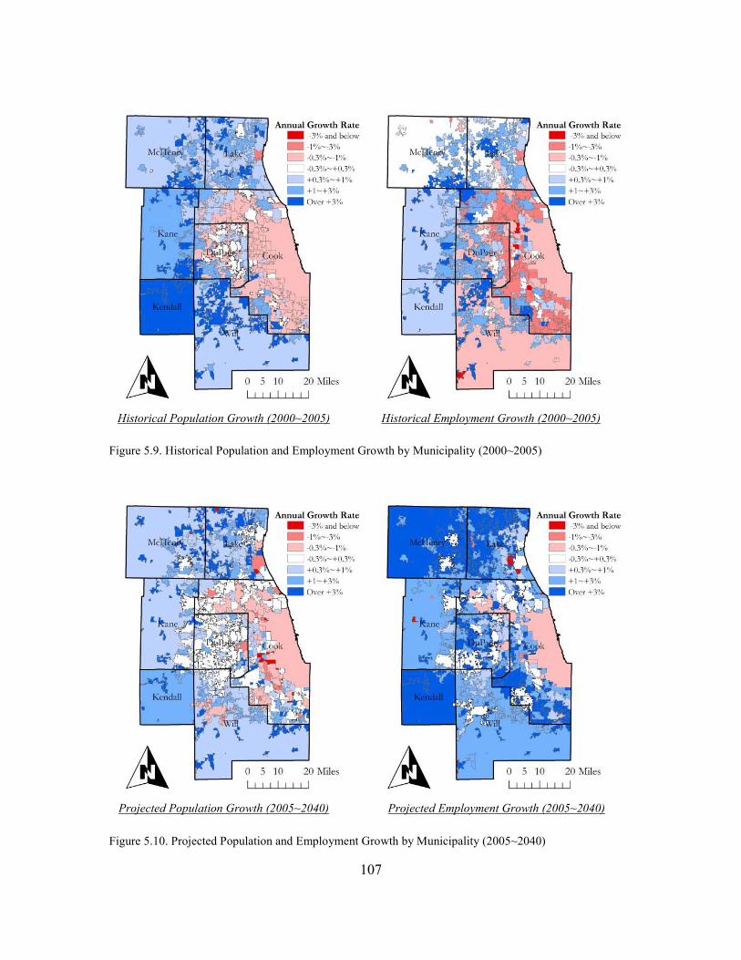
107

Figure 5.9. Historical Population and Employment Growth by Municipality (2000~2005)

Figure 5.10. Projected Population and Employment Growth by Municipality (2005~2040)

Projected Employment Growth (2005~2040) Projected Population Growth (2005~2040)

Historical Employment Growth (2000~2005) Historical Population Growth (2000~2005)

108

5.4. Impact Analysis of Reactive Land Use Regulations

5.4.1. Reactive Land Use Regulations by Suburban Communities

Using the spatial REIM, in this section, a set of impact analyses are conducted to assess the

macroeconomic impacts of some types of reactive land use regulations that limit housing supply

and population growth in the municipalities. Although Chicago has been considered as a less

regulated region compared with many other metropolitan areas, a considerable number of

suburban municipalities have implemented minimum-lot-size zoning ordinances or building

permit caps. According to a recent survey conducted by the Wharton’s residential land use

regulation project in 2005 (Gyourko et al. 2008), among 98 municipalities surveyed (of total 296

entities in this area), 11 cities or towns have at least a two-acre-minimum-lot-size requirement

somewhere within their jurisdictions; and another 5 communities have at least a one-acre-

minimum-lot-size requirement (see figure 5.11). Also, 10 municipalities have one or more

explicit “statutory limits on the number of building permits for single family and multifamily

product, on the number of single-family or multifamily units authorized for construction in any

given year, on the number of multifamily dwellings permitted in the community, or on the

number of units allowed in any given multifamily building” (p.701). Interestingly, there is no

municipality having both restrictions – i.e. 1) two- or one-acre-minimum-lot-size requirement and

2) permit caps – together. This may suggest that the two types of regulations are functioning in a

similar way, that may be limiting population increases as well as housing construction in the

municipality.

As noted, such reactive land use regulations directly affect housing supply and thus population

growth within the jurisdictions; and building permit data shows this deterrent effect.

Municipality-level building permit data were compiled for the Chicago region, provided by U.S.

Census, between 2006 and 2008 to check the effect of the regulations, because the regulation

information is for year 2005. Then, the number of permitted units divided by 2005 population

(on the y-axis) was related to the projected annual population growth rate for the three years (on

the x-axis) for two different groups: 1) municipalities with the minimum-lot-size requirements or

109

permit caps vs. 2) municipalities without such reactive regulations (figure 5.12).46 Two things are

notable. First, x and y show somewhat strong positive relationship, which may imply that the

population growth projected by the spatial REIM correctly forecasts the population changes of

individual municipalities because there appears to be a strong correlation with the observed

building permit data. Secondly, consistent with the expectation, the group of municipalities

having the more reactive regulations shows a flatter slope, which indicates that the number of

building permits tends to be smaller in these communities, when population growth potential is

controlled. In other words, the regulations may have a significant negative effect on local

housing supply.

Figure 5.11. Reactive Land Use Regulations in Chicago

46 Rather than using the number of permitted units as they stand, here I divide the number by the base year population and use the value to control the effects stemming from the size variance. It also needs to be noted that the figure excludes the municipalities where building permit or land use regulation information is not available or 2005 population is smaller than 5,000.

110

Relationship between Population Growth Rate andPer Capita Permitted Units

y = 0.2084x + 0.0091

R2 = 0.2791

y = 0.3373x + 0.0065

R2 = 0.4082

0

0.01

0.02

0.03

0.04

0.05

0.06

0.07

0.08

0.09

0.1

-10.00% -5.00% 0.00% 5.00% 10.00% 15.00% 20.00%

Annual Population Growth Rate (2005~2008)

Number of Permitted Units / 2005 Population Municipalities with the

reactive land useregulations

Municipalities withoutsuch regulations

Linear (Municipalitieswith the reactive landuse regulations)

Linear (Municipalitieswithout suchregulations)

Figure 5.12. Building Permits & Reactive Land Use Regulations

However, the regulations may not always come into effect. There is no reason the regulations

reduce local housing stock or population if there is no demand for new construction. Also, as far

as the new construction plans satisfy the lot-size or permit cap requirements, the regulations will

not limit housing supply and following population increase to that extent. This means that the

presence of the regulations needs to be interpreted in the model as an upper limit of housing stock

or population growth rate rather than a negative shock with a certain magnitude on the variables.

Once the regulations are reflected in this way, mirroring reality, in simulation the potential

negative shock will take effect conditionally with different amounts in different municipalities.47

This issue also highlights that the effects of local land use regulations can be better analyzed by

“modeling and simulation,” particularly a simulation model like the spatial REIM, in which

population by municipality is projected, so that it is possible to identify whether or not the actions

come into effect in a particular locality at a particular time point.

47 The shock will be zero, if a municipality does not satisfy both conditions: 1) the regulations are implemented and 2) population is likely to grow more rapidly than the given upper limit.

111

5.4.2. Prior Experiments: The Effects of a Negative Population Shock at a Particular

Location

As noted, the impact analyses of minimum-lot-size requirements and building caps can be

properly conducted by imposing the upper limit on population increase. Before conducting the

impact analyses, a simple negative population shock to two selected municipalities, one at a time,

will be considered to explore how the impact is spread out over the region’s economy and space

in each case. These experiments will enhance the interpretation of the complicated simulation

outcomes in the main impact analyses, which are a mixture of many different shocks in different

places having the regulations.

More specifically, a negative population shock with the magnitude -1,000 is first given to the

Frankfort village in year 2006; and then the same amount of shock is imposed on the Sugar Grove

village in the same year. According to the Wharton survey, both towns implemented the reactive

regulations as of 2005. At the same time, their population is estimated to grow very rapidly in the

baseline spatial REIM projections.

Figure 13 demonstrates how the population shock affects employment across space in the two

cases. Above all, it is evident that a greater employment loss occurs not only in the very

municipality but also in the places which import the workers from the municipality with a shock,

such as the cities of Chicago, Aurora, and Naperville, because the municipality-level employment

change is linked to the population changes in the labor market areas captured by the spatial

weight matrix based on the journey-to-work data in the modified RDAM. Furthermore, although

small, many other municipalities will experience employment decreases, even though they have

no interaction with the affected municipalities in terms of the journey-to-work flow. This is

attributable not only to the indirect linkages through the power series of spatial weight matrix at

municipality level but also to the systematic interconnections from a municipality to others via

the regional layer.48 In other words, population and employment shock in any part of the region

48 A shock given to a particular municipality first alters the projections of all municipalities with consideration of their spatial interdependence and then changes the values of macroeconomic variables accordingly. In addition, through the iteration of (Step 1) – (Step 3) – (Step 4), population and employment in individual municipalities are further adjusted to determine the probable state of the spatial economic system under the shock which satisfies the modified RDAM as well as all macroeconomic equations at the same time.

112

will alter macroeconomic variables (i.e. decreasing consumption, production, and inter-industry

purchases) and then generate unfavorable effects on all parts of the regional economic system.

Figure 5.13. The Effects of the Population Shock on Employment by Municipality in 2006

Table 5.6 presents the effects of the population shock on regional employment by sector in each

case. First of all, the magnitudes of the impacts in Construction and Trade sectors are larger than

the shares in the base year’s regional employment, listed in table 5.7. In contrast, Manufacturing,

which accounts for 9.5% of regional total employment in the base year, received just about 7.6%

of the total impact in both cases. This is consistent with the intuition that generally a population

shock more profoundly affects the local sectors, that heavily rely on local spending.

In addition, it is clearly shown that the magnitude and composition of overall impacts on regional

employment vary by the location of the shock. Even though the same amount of shock is given

to the population, the effect is greater in the case of Frankfort village than the Sugar Grove village,

probably for two main reasons: 1) Frankfort is more highly interconnected to other places in the

region as a labor supplier and 2) the population shock given to the Frankfort affects the sectors in

The Case of Sugar Grove Village

The Case of Frankfort Village

113

a manner that generates a larger ripple effects on regional employment. The differences in the

composition can be partly explained by the differences in the industry mixes between the two

municipalities and their associated communities (i.e. the places which have tight connections with

the municipality). In other words, the Frankfort’s larger share of Trade sector (18.2%), compared

to that of the Sugar Grove (7.7%) may partly cause the larger impact on Trade sector in the case

of Frankfort village.49

Table 5.6. The Effects of the Population Shock on Regional Employment by Sector

The Case of Frankfort Village The Case of Sugar Grove Village

# % # %

Construction (Sector 5) -63.9 11.5% -54.1 11.3%

Manufacturing (Sector 6~23) -42.4 7.6% -36.3 7.6%

Trade (Sector 24~25) -129.3 23.2% -98.3 20.5%

FIRE (Sector 34~35) -46.5 8.4% -37.5 7.8%

Service (Sector 36~45) -208.1 37.4% -176.8 36.9%

All Other Sectors -66.0 11.9% -76.7 16.0%

Total -556.2 100.0% -479.7 100.0%

Table 5.7. Industry Mixes of the Region and the Two Municipalities

Region as a Whole Frankfort Village Sugar Grove Village

Construction (Sector 5) 5.6% 10.6% 12.5%

Manufacturing (Sector 6~23) 9.5% 12.4% 12.7%

Trade (Sector 24~25) 20.2% 18.2% 7.7%

FIRE (Sector 34~35) 11.3% 8.5% 7.8%

Service (Sector 36~45) 41.2% 40.9% 43.2%

All Other Sectors 12.2% 9.3% 16.0%

Total 100.0% 100.0% 100.0%

Figure 5.14 demonstrates the long-run effect of the shock given in year 2006 on regional

employment. The graph shows that the negative effect on regional employment will be quickly

mitigated in several following years, when a shock is given to a particular year (i.e. Year 2006 in

this case) only. This may be because the regional economic growth is largely determined by the

49 But, for a more complete explanation, consideration needs to be given to the industry mixes of the associated communities and inter-industry linkages of the Chicago economy. In fact, a larger impact on Construction sector is found in the case of Frankfort village, even though the share of the sector is smaller there than the Sugar Grove.

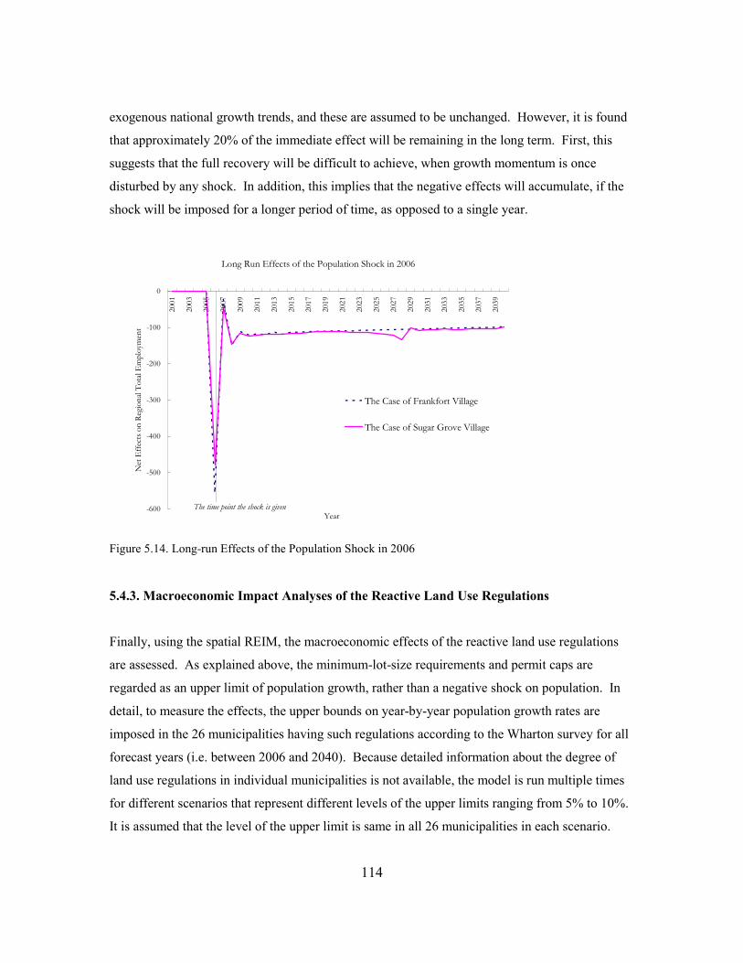
114

exogenous national growth trends, and these are assumed to be unchanged. However, it is found

that approximately 20% of the immediate effect will be remaining in the long term. First, this

suggests that the full recovery will be difficult to achieve, when growth momentum is once

disturbed by any shock. In addition, this implies that the negative effects will accumulate, if the

shock will be imposed for a longer period of time, as opposed to a single year.

Long Run Effects of the Population Shock in 2006

-600

-500

-400

-300

-200

-100

0

2001

2003

2005

2007

2009

2011

2013

2015

2017

2019

2021

2023

2025

2027

2029

2031

2033

2035

2037

2039

Year

Net Effects on Regional Total Employment

The Case of Frankfort Village

The Case of Sugar Grove Village

The time point the shock is given

Figure 5.14. Long-run Effects of the Population Shock in 2006

5.4.3. Macroeconomic Impact Analyses of the Reactive Land Use Regulations

Finally, using the spatial REIM, the macroeconomic effects of the reactive land use regulations

are assessed. As explained above, the minimum-lot-size requirements and permit caps are

regarded as an upper limit of population growth, rather than a negative shock on population. In

detail, to measure the effects, the upper bounds on year-by-year population growth rates are

imposed in the 26 municipalities having such regulations according to the Wharton survey for all

forecast years (i.e. between 2006 and 2040). Because detailed information about the degree of

land use regulations in individual municipalities is not available, the model is run multiple times

for different scenarios that represent different levels of the upper limits ranging from 5% to 10%.

It is assumed that the level of the upper limit is same in all 26 municipalities in each scenario.

115

Figure 5.15 presents the effects of the regulations on employment by municipality, when the

upper limit is set as 5% (i.e. population growth can be attained up to 5%/year in the

municipalities with the regulations.). As shown, in 2006 (the first year with the restriction), the

considerable negative impacts begin to appear in some municipalities, including Frankfort, Sugar

Grove, Chicago, Aurora, Naperville, etc. As discussed in the previous section, these places are

the villages where the projected rapid population growth is limited by the regulations or the cities

that import the workers from the affected villages. Then, in 2040 (the last year in the simulation),

it was found that the employment loss is dramatically expanded across space; most of the

municipalities exhibit employment decline by more than 10 jobs due to the regulations

implemented by a limited number of towns. This expanding negative effect is also clearly

demonstrated in figure 5.16, that shows the long-run effects of the regulations on region-wide

employment level. More specifically, net employment loss in the entire region will reach about

5,500 (approximately 0.1% of total employment) in 2040, if year-by-year population growth rates

are bounded at 5% continuously in the 26 municipalities, due to the regulations. The figure also

indicates that the magnitude of the effect depends on the degree of restrictiveness of the

regulations.

Figure 5.15. The Effects of the Regulations (Upper Limit: 5%) on Employment by Municipality

Figure 5.15. The Long-Run Effects of the Regulations on Regional Employment

The Net Employment Effect in 2040

The Net Employment Effect in 2006

116

Long Run Effects of the Regulations

-6,000

-5,000

-4,000

-3,000

-2,000

-1,000

0

1,000

2001

2003

2005

2007

2009

2011

2013

2015

2017

2019

2021

2023

2025

2027

2029

2031

2033

2035

2037

2039

Year

Net Effects on Regional Total Employment

Upper Limit: 10%

Upper Limit: 9%

Upper Limit: 8%

Upper Limit: 7%

Upper Limit: 6%

Upper Limit: 5%

Forecasts

Figure 5.16. The Long-Run Effects of the Regulations on Regional Employment

Another finding to be noted is that some municipalities appear to achieve employment gains,

compared to the baseline in 2040. Interestingly, the municipality, which achieves the largest job

gain, is the Sugar Grove Village, one of the towns where population growth is limited by its land

use regulation. As demonstrated in figure 5.17, although the village experiences a large negative

effect in a short- and mid-term with a peak loss by about 1,500 in 2025, thereafter, the net effect

starts to decline; and, at the end, its 2040 employment level with the land use regulation is greater

than that in the baseline projection. This can be partly explained when attention is paid to the

population growth trajectories of the village (figure 5.18). In the baseline scenario, its population

rises very rapidly until 2025, but then is stagnant, perhaps due to the depletion of developable

land which is found as an important determinant of local population increase in the modified

RDAM estimation. Given this baseline trajectory, if the pace of population growth is controlled

by the land use regulation, the village will be able to maintain the comparative advantage of

larger developable land, which may be its major growth momentum, for a longer period of time

and achieve extra population and employment growth in the long run. In this sense, the land use

control can be a strategic action to enhance the long-run local growth. However, from the

perspective of the region as a whole, such strategic behaviors of individual local governments

may not be favorable, as confirmed by the found significant regional employment loss.

117

Employment Growth Trajectories of Sugar Grove Village

-4,000

-2,000

0

2,000

4,000

6,000

8,000

10,000

12,000

14,0002001

2003

2005

2007

2009

2011

2013

2015

2017

2019

2021

2023

2025

2027

2029

2031

2033

2035

2037

2039

Year

Employment .

Net Effect

Baseline

Upper Limit: 5%

Forecasts

Figure 5.17. Employment Growth Trajectories of Sugar Grove Village

Population Growth Trajectories of Sugar Grove Village

-30,000

-20,000

-10,000

0

10,000

20,000

30,000

40,000

50,000

2001

2003

2005

2007

2009

2011

2013

2015

2017

2019

2021

2023

2025

2027

2029

2031

2033

2035

2037

2039

Year

Population

.

Net Effect

Baseline

Upper Limit: 5%

Forecasts

Figure 5.18. Population Growth Trajectories of Sugar Grove Village

Table 5.8 summarizes the effects of minimum-lot-size requirements and permit caps on main

macroeconomic variables in the case of 5% upper limit. Consistent with the expectation,

population, which is directly limited by the regulations, show the greatest percentage loss

118

compared to the baseline. Although the magnitudes are smaller, the negative effects are found in

all other variables, such as GRP, production, employment, and income. Particularly, as in the

case of the prior experiments, local sectors’ losses are larger than Manufacturing, which is

relatively less dependent on household spending and local governments’ expenditures. As

demonstrated above, the regional economy will be affected more significantly if the regulations

are implemented in a more restrictive manner. The larger impact is also probable, when a greater

number of municipalities in the region use such reactive land use regulations for their own

interests, as opposed to considering the overall region’s prosperity.

Table 5.8. Macroeconomic Effects of the Regulations: Baseline vs. Upper Limit: 5%

Year 2040

Year 2005

Baseline Upper Limit:

5% Net Effect %

GRP 404,448 832,890 832,451 -438 -0.05%

Population 8,449,379 10,305,923 10,260,947 -44,976 -0.44%

Total Output 921,052 1,851,569 1,850,418 -1,151 -0.06%

Employment 4,813,568 6,309,561 6,304,096 -5,466 -0.09%

Construction (Sector 5) 269,899 324,307 323,968 -338 -0.10%

Manufacturing (Sector 6~23) 455,135 346,076 345,951 -125 -0.04%

Trade (Sector 24~25) 974,122 1,169,071 1,167,585 -1,486 -0.13%

FIRE (Sector 34~35) 541,939 752,546 752,246 -300 -0.04%

Service (Sector 36~45) 1,983,305 2,877,071 2,874,330 -2,741 -0.10%

All Other Sectors 589,168 840,491 840,016 -475 -0.06%

Personal Income 362,000 682,226 681,945 -282 -0.04%

Note: All monetary values are in 2005 chained million dollars.

5.5. Summary & Discussion

This study develops a new integrated multi-level simulation model, a spatial REIM, in which

local- and lower-level dynamics are incorporated into a coupling-type REIM in a reciprocal

interactive manner, as opposed to a top-down allocation process. The integration of the multi-

level variables in a single framework expands the capabilities of the conventional REIM, which is

a macroeconomic tool as it stands by facilitating the development of local-level forecasting and

analysis.

119

In addition, with the established feedback connections from local layer to region-wide variables,

the spatial REIM can support the analysis of the macroeconomic effects of local actions,

particularly land use policies, for which most existing models based on a strict top-down

approach, has limited usefulness.

The spatial REIM was applied to the Chicago metropolitan area in which about three hundred

municipalities with their own local government authorities of, but highly interconnected with

each other as a part of the large single economic system. Furthermore, the applied model is used

to assess the macroeconomic effects of reactive land use regulations (i.e. minimum-lot-size

requirements and building caps), which have been implemented in some suburban communities

in the region. From the impact analyses, it was found that the regulations that bind local housing

supply and population growth within the jurisdictions:

1) generate negative impacts, spread out over space and the economy through the labor

supply chains and inter-industry linkages.

2) dampen the pace of regional economic growth considerably, although the actions are

sometimes favorable to the long-run prosperity of the implementing, individual

municipalities.

3) tend to induce disproportionate impacts on different sectors of the economy – i.e. local

sectors, which heavily depend on household expenditures, are affected more seriously.

4) induce effects that vary substantially by the location of the implementation.

Although the new model and the impact analyses provide additional analytical capabilities for

planning practices and a better understanding of the economic implications of land use

regulations respectively, this study is not without limitations. First of all, when local growth

dynamics are modeled in the Chicago application, attention is only paid to aggregated population

and employment, as opposed to population by group and employment by sector. Without

appropriate consideration of the heterogeneity among various groups of households and

businesses, the model cannot effectively describe the complexity inherent in mobility and

location decision-making processes that vary significantly by industry, firm size, population

cohort, and income group. However, expanding the complexity of the system may generate

instability in the model, as the number of structured equations in the modified RDAM is

increased to capture increased heterogeneity.

120

In addition, the linear fashion of the RDAM formulation, adopted to model the local growth

dynamics, is not ideal for describing the intrinsic non-linearity of a dynamic metropolitan system.

Again, the challenge is the model stability, which is more difficult to be attained with non-linear

forms of dynamic equations.

Moreover, the present version of the spatial REIM employs a modified RDAM, where the spatial

interdependence is represented by a fixed spatial weight matrix, even though it is questionable

that the matrix is a proper representation of true interdependence among municipalities over a

long period of forecast years. The simple cell-level updating module, as opposed to a more

advanced simulation method, is another limitation of the present application. Generally poor

availability of local level economic data is also a challenge to be overcome to better calibrate the

model.

Future research will seek to figure out the effective ways to address these limitations and

challenges in modeling and applications. It is expected that the model will be improved and

become a more competitive analytical tool to fully describe the complexity and dynamics of

spatial economic systems. Then, it will be able to better support various impact and policy

analyses and facilitate informed decision makings.

121

6. SUMMARY & DISCUSSION

6.1. Summary of the Overall Dissertation Research

While changes in the regional economy are sometimes taken into account in connection with land

use changes and the evolution of spatial structure, the reverse connection is rarely, if at all,

studied. To address this shortcoming, throughout the three pieces of research as well as a

literature review in this dissertation, I examine how a regional economy is influenced by

interventions in land development which significantly affect its property markets and overall

spatial structure.

The first study empirically analyzes the potential negative effect of strict land use regulations on

household residential mobility. Here, a correlation analysis first reveals that the metropolitan

areas, where strict land use regulations were implemented in late 1980s, are more likely to exhibit

a lower correlation between intraregional population and employment changes and an increasing

mean commuting time between 1990 and 2000. In addition, the spatial econometric analysis

using a regional disequilibrium adjustment framework shows a lower population adjustment rate

in the regulated regions, which implies lower household mobility in the areas. The findings

suggest that strict regulatory barriers to land development may freeze the local housing supply

and dampen household residential mobility within the region. The affected mobility itself may

indicate the reduced utility of residents. Further, it induces greater spatial mismatches and longer

commuting, which may significantly reduce the efficiency in the operation of the regional

economic system.

In contrast, the second study empirically investigates the potential contribution of land use

planning to uncertainty reduction and a more economically efficient use of land by focusing on

the case of urban fringe land markets where agricultural production is operated under the

uncertainties regarding the timing of potential land development for urban uses. According to the

analysis of land use data in Oregon, the UGBs seem to inform farmland owners’ decision making.

Furthermore, a cross-sectional regression analysis using data for 82 single-county MSAs detects a

positive effect of UGB on agricultural investment levels, suggesting the real contribution of the

122

UGB to uncertainty reduction. The UGB’s effect is found to be statistically significant where

larger shares of livestock and fruit are produced so that farmers are more likely to require

information regarding the timing of development to reduce the risk of overinvestment.

The third study assesses the macroeconomic effects of minimum-lot-size requirements and

building permit caps that have been implemented by some of the suburban communities in the

Chicago metropolitan area. This is accomplished by employing a new integrated simulation

model in which region-wide, local, and cell-level variables are interacted with each other in a

reciprocal manner, as opposed to traditional ‘top down’ approach. The restrictive regulations are

found to impede regional economic growth by constraining local housing supply and population

growth within the places, although the regulations sometimes enhance the long-run prosperity of

the implementing, individual municipalities.

6.2. Policy Implications of the Findings

The implications of the findings for land use planning and policy reform appear great. By

showing some empirical analysis outcomes that suggest the negative effect of strict land use

regulations on local housing supply and household residential mobility, the study on land use

regulations and intraregional job-people interactions cautions land use planners or policy makers.

Also the study raises an important issue: how can we minimize the delay of the development

process and impact on housing supply, while maintaining the contribution of interventions to

addressing market failures and realizing a well-organized spatial structure? Is it desirable to add

another layer of regulation (e.g. mixed use zoning or affordable housing requirements) to deal

with the problem? Alternatively, do we need to remove some of the regulatory barriers? What

type of institutional reform will be effective in shortening the delay of the development process?

Do we need to advocate market-based approaches over traditional location-specific regulations?

Future research that tackles such questions may be helpful for shedding light on this important

issue.

The second study emphasizes the benefits of land use planning practice with respect of

information production and distribution, which have been largely ignored. Given that land

123

markets and development processes generally bear significant transaction costs due to intrinsic

uncertainties, we need to pay more attention to how we can reduce the uncertainty and realize a

more efficient development process and land use effectively through land use planning practice.

In this regard, planners need to make an effort to identify and target the situations in which

uncertainties and transaction costs prevent an efficient use of land resources. For instance, they

need to think about why many brownfield sites are less likely to be redeveloped. Do we have to

facilitate redevelopment only by using financial incentives? Or, can we deal with the problem

effectively by addressing the lack and asymmetry of information regarding the sites? Moreover,

we need to seek a better institutional arrangement in which information is more efficiently

produced and distributed.

The third research also provides some lessons for planners and policy makers. Given that land

use controls in a particular municipality are found to have significant effects on other places and

the overall regional economy, land use planning practice and regulation enforcement at local level

needs to be better coordinated and conducted with proper consideration of region-wide concerns.

This is required not only for unregulated places but also for the municipality itself, because every

locality as a part of the regional economic system, highly interrelated with each other, so that a

negative effect spilling over to others is likely to return. The third study highlights the analytic

needs for dealing with the interrelationships among municipalities and ‘land use – regional

economy’ interactions. Without an analytic tool, in which the behavior of a spatial economic

system is well described, it is difficult to assess the potential effects of various policy options and,

consequently, hard to attain informed policy decision making that is essential not only for

effective land use management but also for regional economic development.

One final point to be stressed is that the economic consequences of land use planning and

regulations are found to highly depend on context. As presented in the study on the contribution

of land use planning to uncertainty reduction, the UGB’s positive effect on agricultural

investment is more likely to be realized in the regions where the items that require a large amount

of sunk costs and a long period of operation are mainly cultivated. The real economic benefits of

the UGB in farmland use may be very small in crop-dominant contexts, although its contribution

with many other aspects would exist. In addition, as discussed and demonstrated in chapter 5, the

124

effect of minimum-lot-size requirements and permit caps significantly vary by the location and

time of the intervention.

This suggests that linking land use planning and regulation to economic development requires

context-based management of land use that promotes potential positive effects and/or dampens

negative effects of interventions rather than simply reducing government interventions in land

development or trying to articulate a one-size-fits-all policy approach. To achieve a more

systematic coordination of economic development and land use planning, attention needs to be

paid to how and why policy outcomes vary by context. In what circumstances are containment

programs more likely to bring a greater efficiency gains in public service provision or

agglomeration benefits, rather than generating housing affordability problems? When does

mixed-use zoning really contribute to reducing auto-based travel, rather than merely acting as an

additional regulatory barrier? To what degree and how can state or regional government bodies

lead and guide local land use planning practices in order to facilitate the systematic cooperation

of localities, rather than harming local autonomy? Future research to answer such questions is

needed in order to fully understand the relationship between land use policies and regional

economic development.

6.3. Limitations and Future Research

The present dissertation research finds a set of significant causal links from land use to the

performance of regional economy. In addition, as explained above, the findings provide

meaningful policy lessons and highlight the issues that need to be considered in order for us to

improve current land use planning practice. However, the studies are not without limitations.

As noted in chapter 3, the first study suffers from the invalid estimation outcomes for many

metropolitan areas, so that the results are not fully conclusive. In addition, the causality (i.e.

whether the strict land use regulations are really responsible for the lower household mobility in

the areas or not) is still remaining untested, although the evidence suggests that this may be the

case. The design of the spatial econometric analysis, where only aggregate population and

employment are considered, also needs to be extended to better assess heterogeneous household

125

and business mobility and their location choices. Moreover, the measurement of the land use

regulations, namely a single index, is another limitation of the study to be improved in the future

research.

Similar limitations exist in the second study. Although the UGB may qualitatively differ by

regions, the UGB establishment practice is considered by using a single dummy variable. The

use of investment in “machinery and equipment” as dependent variable is also an unsatisfactory

feature of the regression analysis, stemming from the data availability, because this type of

investment is relatively less irreversible compared to long-term soil improvement or building

construction for agricultural purposes.

Although the third study develops a new analytic framework, which can be employed for the

economic impact analysis of local land use policies, the Chicago application as well as the model

itself needs to be extended in many respects, as discussed in the discussion part of chapter 5.

Particularly, the spatial REIM can better support planning practices, once it can properly deal

with various groups of households and businesses, the non-linearity of growth dynamics, the

evolving spatial interdependence among the municipalities of interest, etc.

Future research will strive toward overcoming these limitations of each study. Further, attention

also will be paid to the policy questions derived from the findings of these studies. By doing this,

it will be possible to obtain a better understanding of the ‘bottom-up’ causal connections of how a

change or intervention in land use influences regional economic performance. Then, land use

planning practice and economic development initiatives can be coordinated more systematically,

leading a more complete realization of urban development that is economically prosperous and, at

the same time, ecologically sustainable.

126

REFERENCES

Alexander, E.R. 1992. A transaction cost theory of planning. Journal of the American Planning

Association 58 (2):190–200. Alexander, E.R. 1994. To plan or not to plan, that is the question: Transaction cost theory and its

implications for planning. Environment and Planning B: Planning and Design 21 (3): 341–352.

Alexander, E.R. 2001. Why planning vs. markets is an oxymoron: Asking the right question. Planning and Markets 4: 1–6. http://www-pam.usc.edu/volume4/v4i1a2print.html

American Institute of Planners. 1976. Survey of State Land Use Planning Activity, Department of Housing and Urban Development, Washington, DC.

Anas, A. and I. Kim. 1996. General equilibrium models of polycentric urban land use with endogenous congestion and job agglomeration. Journal of Urban Economics 40 (2): 232-256.

Anas, A. and R. Xu. 1999. Congestion, land use, and job dispersion: A general equilibrium model. Journal of Urban Economics 45 (3): 451-473.

Anas, A. and Y. Liu. 2007. A Regional Economy, Land Use, and Transportation model (RELU-TRAN©): Formulation, algorithm design, and testing. Journal of Regional Science 47 (3): 415-455.

Anderson, H. A. 1999. Use and Implementation of Urban Growth Boundaries, Center for Regional and Neighborhood Action, Denver at http://www.colorado.edu/conflict/5010/CRNA-UGBReport.pdf

Anthony, J. 2003. The effects of Florida’s growth management act on housing affordability. Journal of the American Planning Association 69 (3): 282–295.

Arnott, R. J. and F. D. Lewis. 1979. The transition of land to urban use, Journal of Political Economy 87 (1): 161-169.

Bailey, M. J. 1959. Note on the economics of residential zoning and urban renewal. Land Economics 35 (3): 288–292.

Barnard, C. H. and W. R. Butcher. 1989. Landowner characteristics: A basis for locational decisions in the urban fringe. American Journal of Agricultural Economics 71 (3): 679-684.

Begg, I. 1999. Cities and competitiveness. Urban Studies 36 (5–6): 795–809. Berry, C. 2001. Land use regulation and residential segregation: Does zoning matter. American

Law and Economics Review 3 (2): 251–274. Besley, T. 1995. Property rights and investment incentives: Theory and evidence from Ghana.

The Journal of Political Economy 103 (5): 903–937. Boarnet, M. G. 1994a. An empirical model of intrametropolitan population and employment

growth. Papers in Regional Science 73 (2): 135-152. Boarnet, M. G. 1994b. The monocentric model and employment location. Journal of Urban

Economics 36 (1): 79-97. Boarnet, M. G., S. Chalermpong, and E. Geho. 2005. Specification issues in models of population

and employment growth. Papers in Regional Science 84 (1): 21-46. Bollinger, C. and K. R. Ihlanfeldt. 1997. The impact of rapid rail transit on economic

development: The case of Atlanta’s MARTA. Journal of Urban Economics 42 (2): 179-204.

Bockstael, N. E. 1996. Modeling economics and ecology: The importance of a spatial perspective. American Journal of Agricultural Economics 78 (5): 1168-1180.

127

Bramley, G. and C. Lambert. 2002. Managing urban development: Land use planning and city competitiveness. In I. Begg, Ed. Urban competitiveness: Policies for dynamic cities. 283-310. Bristol, UK: The Policy Press.

Brueckner, J. K. 1990. Growth controls and land values in an open city. Land Economics 66 (3): 237-248.

Buitelaar, E. 2004. A transaction-cost analysis of the land development process. Urban Studies 41 (13): 2539–2553.

Burby, R. J., A. C. Nelson, D. Parker, and J. Handmer. 2001. Urban containment policy and exposure to natural hazards: Is there a connection? Journal of Environmental Planning and Management 44 (4): 475-490.

Burchell, R. W., A. Downs, and B. McCann, eds. 2005. Sprawl costs: Economic impacts of unchecked development, Washington, DC: Island Press.

Burchell, R. W., N. A. Shad, D. Listokin, eds. 1998. The costs of sprawl – Revisited. Washington, DC: National Academy Press.

Burnell, J. D. 1985. Industrial land use, externalities, and residential location. Urban Studies 22 (5): 399–408.

Buzbee, W. W. 2005. The regulatory fragmentation continuum, westway and the challenges of regional growth. Journal of Law and Politics 21: 323-364.

Cameron, G. and J. Muellbauer. 1998. The housing market and regional commuting and migration choices. Scottish Journal of Political Economy 45 (4): 420-446.

Campbell, S. 1996. Green cities, growing cities, just cities?: Urban planning and the contradictions of sustainable development. Journal of the American Planning Association 62 (3): 296-312

Calzonetti, F. J. and R. T. Walker. 1991. Factors affecting industrial location decisions: A survey approach. In H.W. Herzog, Jr. and A.M. Schlottmann, Ed. Industrial Location and Public Policy. 221-240. Knoxville, TN: The University of Tennessee Press.

Capozza, D. R. and R. W. Helsley. 1990. The stochastic city. Journal of Urban Economics 28 (2): 187-203.

Carlino, G. A. and E. S. Mills. 1987. The determinants of county growth. Journal of Regional Science 27 (1): 39-54.

Carruthers, J. I. 2003. Growth at the fringe: The influence of political fragmentation in United States metropolitan areas. Papers in Regional Science 82 (4): 475–499.

Carruthers, J. I. and G. F. Ulfarsson. 2002. Fragmentation and sprawl: Evidence from interregional analysis. Growth and Change 33 (3): 312–340.

Carruthers, J. I. and G. F. Ulfarsson. 2003. Urban sprawl and the cost of public services. Environment and Planning B: Planning and Design 30 (4): 503–522.

Carruthers, J. I. and G. F. Mulligan. 2007. Land absorption in U.S. metropolitan areas: Estimates and projections from regional adjustment models. Geographical Analysis 39 (1): 78-104.

Cervero, R. 2001. Efficient urbanisation: Economic performance and the shape of the metropolis. Urban Studies 38 (10): 1651-1671.

Cervero, R. and M. Duncan. 2006. Which reduces vehicle travel more: Jobs-housing balance or retail-housing mixing? Journal of the American Planning Association 72 (4): 475-490.

Cervero, R. and K. Kockelman. 1997. Travel demand and the 3Ds: Density, diversity, and design. Transportation Research Part D: Transport and Environment 2 (3): 199–219.

Cheshire, P. C. and C.A.L. Hilber. 2008. Office space supply restrictions in Britain: The political economy of market revenge. The Economic Journal 118 (529): F185–F221.

Cheshire, P. C. and S. Sheppard. 2005. The introduction of price signals into land use planning decision-making: A proposal. Urban Studies 42 (4): 647–663.

128

Clark, T. N. 1988. The fiscal austerity and urban innovation project. Political Science and Politics 21 (1): 94-98.

Ciccone, A. and R. E. Hall. 1993. Productivity and the density of economic activity. NBER Working Paper No. 4313, National Bureau of Economic Research.

Crecine, J. P., O. A. Davis, and J. E. Jackson. 1967. Urban property markets: Some empirical results and their implications for municipal zoning. Journal of Law and Economics 10: 79–99.

Crane, R. 2000. The influence of urban form on travel: An interpretive review. Journal of Planning Literature 15 (3): 2-23.

Conway, R. S. Jr. 1990. The Washington projection and simulation model: A regional inter-industry econometric model. International Regional Science Review 13 (1-2): 141-166.

Correll, M. R., J. H. Lillydahl, and L. D. Singell. 1978. The effects of greenbelts on residential property values: Some findings on the political economy of open space. Land Economics 54 (2): 207–217.

D’Arcy, E. and G. Keogh. 1999. The property market and urban competitiveness: A review. Urban Studies 36 (5-6): 917–928.

Davis, O. A. 1963. Economic elements in municipal zoning decisions. Land Economics 39 (4): 375–386.

Dawkins, C. J. 2000. Transaction costs and the land use planning process. Journal of Planning Literature 14 (4): 507–518.

Dawkins, C. J. and A. C. Nelson. 2003. State growth management programs and central-city revitalization. Journal of the American Planning Association 69 (4): 381–396.

Deal, B., J. Kim, and A. Chakraborty. 2009. Growth management and sustainable transport: Do growth management policies promote transit use? Journal of Public Transportation 12 (4): 21-40.

Dhillon, P. S. and D. A. Derr. 1974. Critical mass of agriculture and the maintenance of productive open space. Journal of the Northeastern Agricultural Economics Council 3 (1): 23-34.

Do, Q. T. and L. Iyer. 2003. Land rights and economic development: Evidence from Vietnam. World Bank Policy Research Working Paper No. 3120. http://www-wds.worldbank.org/servlet/WDSContentServer/WDSP/IB/2003/09/23/000094946_03091104055746/Rendered/PDF/multi0page.pdf

Donaghy, K. P., N. Balta-Ozkan, and G. J. D. Hewings. 2007. Modeling unexpected events in temporally disaggregated econometric input-output models of regional economies. Economic Systems Research 19 (2): 125-145.

Downs, A. 1991. The advisory commission on regulatory barriers to affordable housing: Its behavior and accomplishments. Housing Policy Debate 2 (4): 1095–1137.

Downs, A. 2002. Have housing prices risen faster in Portland than elsewhere? Housing Policy Debate 13 (1): 7–31.

Engle, R., P. Navarro, and R. Carson. 1992. On the theory of growth controls. Journal of Urban Economics 32 (3): 269-283.

Evans, A. W., 2002. Building Jerusalem: Can Land Use Planning Affect Economic Growth?, Conference Paper CP02A11, Lincoln Institute of Land Policy.

Evans, A. W. 2004. Economics and Land Use Planning. Oxford: Blackwell Publishing. Ewing, R. H. 1996. Characteristics, causes, and effects of sprawl: A literature review.

Environmental and Urban Studies 21 (2): 1–15. Ewing, R. and R. Cervero. 2001. Travel and the built environment: A synthesis. Transportation

Research Record 1780: 87–114.

129

Ewing, R. H., R. Pendall, and D. Chen. 2002. Measuring sprawl and its impact, Washington, DC: Smart Growth America http://smartgrowthamerica.org/sprawlindex/MeasuringSprawlTechnical.pdf

Fair, R. C. and D. M. Jaffee. 1972. Methods of estimation for markets in disequilibrium. Econometrica 40 (3): 497–514.

Feder, G. and D. Feeny. 1991. Land tenure and property rights: Theory and implications for development policy. The World Bank Economic Review 5 (1): 135–153.

Feser, E. and A. Isserman. 2005. Urban spillovers and rural prosperity. http://www.urban.uiuc.edu/faculty/feser/Pubs/Urban_spillovers_and_rural_prosperity.pdf

Fischel, W. A. 1980. Zoning and the exercise of monopoly power: A reevaluation. Journal of Urban Economics 8 (3): 283-293.

Fischel, W. A. 1985. The Economics of Zoning Laws: A Property Rights Approach to American Land Use Controls, Baltimore: The Johns Hopkins University Press.

Fischel, W. A. 1999. Zoning and land use regulation. In B. Bouckaert and G. D. Geest, Ed. The Encyclopedia of Law and Economics. New Jersey: Edward Elgar.

Fisher, W. D. and M. C. L. Fisher. 1975. The spatial allocation of employment and residence within a metropolitan area. Journal of Regional Science 15 (3): 261-276.

Foster, K. A. 2001. Regionalism on Purpose, Cambridge, MA: Lincoln Institute of Land Policy. Friend, J.K. and W.N. Jessop. 1969. Local government and strategic choice: An operational

research approach to the processes of public planning, Beverly Hills: Sage Publications. Frigg, R. and S. Hartmann. 2006. Models in science. Stanford Encyclopedia of Philosophy.

http://plato.stanford.edu/entries/models-science/. Fulton, W., R. Pendall, and M. Nguyen, eds. 2001. Who sprawls the most? How growth patterns

differ across the U.S., Bookings Institution. http://www.brookings.edu/es/urban/publications/fulton.pdf

Gale, D. E. 1992. Eight state-sponsored growth management programs: A comparative analysis. Journal of the American Planning Association 58 (4): 425-439.

Gardner, B. D. 1977. The economics of agricultural land preservation. American Journal of Agricultural Economics 59 (5): 1027–1036.

Gibb, K., D. Mackay, and M. White. 2002. The property sector and its role in shaping urban competitiveness: A selective review of literature and evidence. In I. Begg, Ed. Urban competitiveness: Policies for dynamic cities. 81–100. Bristol, UK: The Policy Press.

Glaeser, E. L. and M. E. Kahn. 2003. Sprawl and urban growth, Discussion Paper No. 2004, Harvard Institute of Economic Research. http://www.economics.harvard.edu/pub/hier/2003/HIER2004.pdf

Glaeser, E. L. 2006. The economic impact of restricting housing supply. Policy Briefs PB-2006-3, Rappaport Institute for Greater Boston, Harvard University. http://www.hks.harvard.edu/rappaport/downloads/policybriefs/glaeserhousing_final.pdf

Glaeser, E. L., J. Gyourko, and R. E. Saks. 2006. Urban growth and housing supply. Journal of Economic Geography 6 (1): 71–89.

Gordon, P. and H. W. Richardson. 1997. Are compact cities a desirable planning goal? Journal of the American Planning Association 63 (1): 95-106.

Governor’s Office of Planning and Research (GOP&R), State of California. 1999. The California Planners’ Book of Lists 1999 http://ceres.ca.gov/planning/bol/1999/

Green, E. K., S. Malpezzin, and S. K. Mayo. 2005. Metropolitan-specific estimates of the price elasticity of supply of housing, and their sources. American Economic Review 95 (2): 334–339.

130

Gyourko, J. Saiz, A. and A. Summers. 2008. A new measure of the local regulatory environment for housing markets: The Wharton residential land use regulatory index. Urban Studies 45 (3): 693-729

Hamilton, B. W. 1978. Zoning and the exercise of monopoly power. Journal of Urban Economics 5 (1): 116-130.

Hanushek, E. A. and J. M. Quigley. 1990. Commercial land use regulation and local government finance. The American Economic Review 80 (2): 176–180.

Heikkila, E. J. 1996. Are municipalities Tieboutian clubs? Regional Science and Urban Economics 26 (2): 203-226.

Henneberry, J., T. McGough, and F. Mouzakis. 2005. Estimating the impact of planning on commercial property markets. In D. Adams, C. Watkins, and M. White, Ed. Planning, Public Policy and Property Markets. 105–127. Oxford: Blackwell Publishing.

Henry, M. S. , B. Schmitt, and V. Piguet. 2001. Spatial econometric models for simultaneous systems: Application to rural community growth in France. International Regional Science Review 24 (2): 171-193.

Henry, M. S. , D. L. Barkley, and S. Bao. 1997. The hinterland’s stake in metropolitan growth: Evidence from selected southern regions. Journal of Regional Science 37 (3): 479-501.

Hewings, G. J. D., M. Sonis, J. Guo, P. R. Israilevich and G. R. Schindler. 1998. The hollowing out process in the Chicago economy, 1975-2015. Geographical Analysis 30 (3): 217-233.

Hopkins, L. D. 2001. Urban development: The logic of making plans. Washington, DC: Island Press.

Hughes, W. T. Jr. and C. F. Sirmans. 1992. Traffic externalities and single-family housing prices. Journal of Regional Science 32 (4): 487–500.

Hunt, J. D., D. S. Kriger, and E. J. Miller. 2005. Current operational urban land use – transport modelling frameworks: A review. Transport Reviews 25 (3): 329-376.

Ihlanfeldt, K. R. 2004. Exclusionary land-use regulations within suburban communities: A review of the evidence and policy prescriptions. Urban Studies 41 (2): 261–283.

Ihlanfeldt, K. R. 2007. The effect of land use regulation on housing and land prices. Journal of Urban Economics 61 (3): 420-435.

Ihlanfeldt, K. R. and T. P. Boehm. 1987. Government intervention in the housing market: An empirical test of the externalities rationale. Journal of Urban Economics 22 (3): 276–290.

Ihlanfeldt, K. R. and D. L. Sjoquist. 2000. Geographic mismatch between jobs and housing. In D. L. Sjoquist, Ed. The Atlanta Paradox. 116–157. New York: Russell Sage Foundation.

Innes, J. E. 1992. Group processes and the social construction of growth management. Journal of the American Planning Association 58 (4): 440-453.

Irwin, E. G. and J. Geoghegan. 2001. Theory, data, methods: Developing spatially explicit economic models of land use change. Agriculture, Ecosystems, and Environment 85 (1-3), 7-23.

Israilevich, P. R., G. J. D. Hewings, G. R. Schindler, and R. Mahidhara. 1996. The choice of input–output table embedded in regional econometric input–output models. Papers in Regional Science 75 (2): 103-119.

Israilevich, P. R., G. J. D. Hewings, M. Sonis, and G. R. Schindler. 1997. Forecasting structural change with regional econometric input-output model. Journal of Regional Science 37 (4): 565-590.

Jaeger, W. K. 2006. The effects of land-use regulations on property values. Environmental Law 26: 105-130.

Jun, M. J. 2004. The effects of Portland’s urban growth boundary on urban development patterns and commuting. Urban Studies 41 (7): 1333–1348.

131

Kaiser, E. J. and D. R. Godschalk. 1995. Twentieth Century land use planning: A stalwart family tree. Journal of the American Planning Association 61 (3): 365-385.

Katz, L. and K. T. Rosen. 1987. The interjurisdictional effects of growth controls on housing prices. Journal of Law and Economics 30: 149-160.

Kelejian, H. H. and D. P. Robinson. 1993. A suggested method of estimation for spatial interdependent models with autocorrelated errors, and an application to a county expenditure model. Papers in Regional Science 72 (3): 297-312.

Kelejian, H. H. and I. R. Prucha. 1998. A generalized spatial two-stage least squares procedure for estimating a spatial autoregressive model with autoregressive disturbances. Journal of Real Estate Finance and Economics 17 (1):99-121.

Kelejian, H. H. and I. R. Prucha. 1999. A generalized moments estimator for the autoregressive parameter in a spatial model. International Economic Review 40 (2): 509-533.

Kim, J. and G. J. D. Hewings. 2010 (forthcoming). Framing urban systems and planning concerns as a multi-level problem: A review of the integrated urban system models with an emphasis on their hierarchical structures. In N. Brooks, K. Donaghy, and G. Knaap, Ed. Oxford University Press Handbook of Urban Economics and Planning.

Kline, J. D. and R. J. Alig. 1999. Does land use planning slow the conversion of forest and farm lands? Growth and Change 30 (1): 3–22.

Knaap, G. J. 1985. The price effects of urban growth boundaries in metropolitan Portland, Oregon. Land Economics 61 (1), 26-35.

Knaap, G. J., C. Ding, and L. D. Hopkins. 2001. Do plans matter? The effects of light rail plans on land values in station areas. Journal of Planning Education and Research 21 (1): 32–39.

Knaap, G. J., L. D. Hopkins, and K. P. Donaghy. 1998. Do plans matter? A game-theoretic model for examining the logic and effects of land use planning. Journal of Planning Education and Research 18 (1): 25-34.

Knaap, G. J. and A. C. Nelson. 1992. The regulated landscape: Lessons on state land use planning from Oregon. Cambridge: Lincoln Institute of Land Policy.

Knaap, G. J. and Y. Song. 2004. The transportation – land use policy connection. Paper prepared for the conference entitled “Access to Destination: Rethinking the Transportation Future of Our Region” http://www.smartgrowth.umd.edu/research/researchpapers-landuseandenvironment.htm

Krabben, E. V. D. and F. Bokema. 1994. Missing links between urban economic growth theory and real estate development processes: Economic growth and building investments in the City of ‘s-Hertogengbosch ., Journal of Property Research 11 (2): 111-129.

Lafferty, R. N. and H. E. Frech. 1978. Community environment and the market value of single family homes: The effect of the dispersion of land uses. Journal of Law and Economics 21 (2): 381-394.

Lai, F. and S. Yang. 2002. A view on optimal urban growth controls. The Annals of Regional Science 36 (2): 229-238.

Lee, D. B. Jr. 1981. Land use planning as a response to market failure. In J. I. de Neufville, Ed. The Land Use Policy Debate in the United States. 149–164. New York: Plenum Press.

Levine, J. 1998. Rethinking accessibility and jobs–housing balance. Journal of the American Planning Association 64 (2): 133-149.

Levine, J. 2006. Zoned out: Regulation, markets, and choices in transportation and metropolitan land-use. Washington, DC: RFF Press.

Levine, N. 1999. The effects of local growth controls on regional housing production and population redistribution in California. Urban Studies 36 (12): 2047–2068.

132

Lichtenberg, E., C. Tra, and I. Hardie. 2007. Land use regulation and the provision of open space in suburban residential subdivisions. Journal of Environmental Economics and Management 54 (2): 199-213.

Linneman, P. and A. Summers. 1991. Wharton Urban Decentralization Project Data Set, Wharton Real Estate Unit, University of Pennsylvania.

Lopez, R. A., A. O. Adelaja, and M. S. Andrews. 1988. The effects of suburbanization on agriculture. American Journal of Agricultural Economics 70 (2), 346-358.

Lynch, L. and J. Carpenter. 2003. Is there evidence of a critical mass in the Mid-Atlantic agriculture sector between 1949 and 1997? Agricultural and Resource Economics Review 32 (1): 116-128

Malpezzi, S. 1996. Housing prices, externalities, and regulation in U.S. metropolitan areas. Journal of Housing Research 7 (2): 209–241.

Mark, J. H. and M. A. Goldberg. 1986. A study of the impacts of zoning on housing values over time. Journal of Urban Economics 20 (3): 257–273.

Maser, S. M., W. H. Riker, and R. N. Rosett. 1977. The effects of zoning and externalities on the price of land: An empirical analysis of Monroe County, New York. Journal of Law and Economics 20 (1): 111–132.

Mayer, C. J. and C. T. Somerville. 2000. Land use regulation and new construction. Regional Science and Urban Economics 30 (6): 639–662.

McDonald, J. F. and D. P. McMillen. 2004. Determinants of suburban development controls: A Fischel expedition. Urban Studies 41 (2): 341-361.

McKinney, M. and K. Essington. 2006. Learning to think and act like a region. Land Lines 18 http://www.lincolninst.edu/pubs/PubDetail.aspx?pubid=1079

Moe, R. and C. Wilkie. 1997. Changing Places: Rebuilding Community in the Age of Sprawl, New York: Henry Holt and Company.

Moore, T. 1978. Why allow planners to do what they do?: A justification from economic theory. Journal of the American Institute of Planners 44 (4): 387–398.

Moore, T. and A.C. Nelson. 1994. Lessons for effective urban containment and resource land preservation policy. Journal of Urban Planning and Development 120 (4): 157–171.

Mulligan, G. F., A. C. Vias, and S. M. Glavac. 1999. Initial diagnostics of a regional adjustment model. Environment and Planning A 31: 855-876.

Muro, M. and R. Puentes. 2004. Investing in a better future: A review of the fiscal and competitive advantages of smarter growth development patterns, Brookings Institution. http://www.brookings.edu/urban/pubs/200403_smartgrowth.pdf

Nelson, A. C. 1999. Comparing states with and without growth management: Analysis based on indicators with policy implications. Land Use Policy 16 (2): 121–127.

Nelson, A. C., R. J. Burby, E. Feser, eds. 2004. Urban containment and central-city revitalization. Journal of the American Planning Association 70 (4): 411–425.

Nelson, A. C. and J. B. Duncan. 1995. Growth Management: Principles and Practice, Chicago: Planners Press.

Nelson, A. C. and T. Moore. 1993. Assessing urban growth management: The case of Portland, Oregon, the USA’s largest urban growth boundary. Land Use Policy 10 (4): 293–302.

Nelson, A. C. and D. R. Peterman. 2000. Does growth management matter? The effect of growth management on economic performance. Journal of Planning Education and Research 19 (3): 277–285.

Netusil, N. R. 2005. The effect of environmental zoning and amenities on property values: Portland, Oregon. Land Economics 81 (2): 227–246.

133

Ohls, J. C. and D. P. Pines. 1975. Discontinuous urban development and economic efficiency. Land Economics 51 (3): 224-234.

Okuyama, Y., G. J. D. Hewings, M. Sonis, and P. R. Israilevich. 2002. An economic analysis of bi-proportional properties in an input-output system. Journal of Regional Science 42 (2): 361-387.

Okuyama, Y., M. Sonis and G. J.D. Hewings. 2006. Typology of structural change in a regional economy: A temporal inverse analysis. Economic Systems Research 18 (2): 133-153.

1000 Friends of Oregon. 1982. Making land use planning a part of the solution to Oregon’s economic recovery: A two year plan, Portland, OR.

Parr, J. B. 1979. Regional economic change and regional spatial structure: Some interrelationships. Environment and Planning A 11: 825-837.

Parr, J. B. 1987. The development of spatial structure and regional economic growth. Land Economics 63 (2): 113-127.

Pendall, R. 1999. Do land-use controls cause sprawl? Environment and Planning B: Planning and Design 26 (4): 555–571.

Pendall, R. 2000. Local land use regulation and the chain of exclusion. Journal of the American Planning Association 66 (2): 125-142.

Pendall, R., R. Puentes, and J. Martin. 2006. From Traditional to Reformed: A Review of the Land Use Regulations in the Nation’s 50 largest Metropolitan Areas, Brookings Institution.

Phillips, J. and E. Goodstein. 2000. Growth management and housing prices: The case of Portland, Oregon. Contemporary Economic Policy 18 (3): 334–344.

Platt, R. H. 1996. Land use and society: Geography, law, and public policy, Washington, DC: Island Press.

Pogodzinski, J. M. and T. R. Sass. 1991. Measuring the effects of municipal zoning regulations: A survey. Urban Studies 28 (4): 597–621.

Pollakowski, H. O. and S. M. Wachter. 1990. The effects of land-use constraints on housing prices. Land Economics 66 (3): 315–324.

Quigley, J. M. and S. Raphael. 2004. Is housing unaffordable? Why isn’t it more affordable? Journal of Economic Perspectives 18 (1): 191–214.

Quigley, J. M. and L. A. Rosenthal. 2005. The effects of land use regulation on the price of housing: What do we know? What can we learn? Cityscape: A Journal of Policy Development and Research 8 (1): 69–137.

Randolph, J. 2004. Environmental Land Use Planning and Management, Washington D.C.: Island Press.

Razin, E. and M. Rosentraub. 2000. Are fragmentation and sprawl interlinked?: North American evidence. Urban Affairs Review 35 (6): 821–836.

Reilly, W. K. [eds.] 1973. The Use of Land: A Citizens’ Policy Guide to Urban Growth, A Task Force Report Sponsored by the Rockefeller Brothers Fund, New York: Thomas Y. Crowell Co.

Rey S. J. 1998. The performance of alternative integration strategies for combining regional econometric and input-output models. International Regional Science Review 21 (1): 1-35.

Rey, S. J. 2000. Integrated regional econometric + input-output modeling: Issues and opportunities. Papers in Regional Science 79 (3): 271-292.

Rey, S. J. and M. G. Boarnet. 2004. A taxonomy of spatial econometric models for simultaneous equations systems. In L. Anselin, R. J. G. M. Florax, and S. J. Rey, Ed. Advances in Spatial Econometrics: Methodology. Springer-Verlag: Berlin.

134

Rey, S. J and B. Dev. 1997. Integrating econometric and input-output models in a multiregional context. Growth and Change 28 (2): 222-243.

Rodriguez, D. A., F. Targa and S. A. Aytur. 2006. Transport implications of urban containment policies: A study of the largest twenty-five U.S. metropolitan areas. Urban Studies 43 (10): 1879-1897.

Rose, L. A. 1989. Urban land supply: Natural and contrived restrictions. Journal of Urban Economics 25 (3): 325-345.

Ross, S. and J. Yinger. 1999. Sorting and voting: A review of the literature on urban public finance. In P. Cheshire and E. S. Mills, Ed. Handbook of Regional and Urban Economics Vol. 3. New York: North-Holland.

Rudel, T. K. 1989. Situations and Strategies in American Land Use Planning, New York: Cambridge University Press.

Rueter, F. H. 1973. Externalities in urban property markets: An empirical test of the zoning ordinance of Pittsburgh. Journal of Law and Economics 16 (2): 313–349.

Sakashita, N. 1995. An economic theory of urban growth control. Regional Science and Urban Economics 25 (4): 427-434.

Saks, R. E. 2008. Job creation and housing construction: Constraints on metropolitan area employment growth. Journal of Urban Economics 64 (1): 178–195.

Sanyal, B. 2000. “Planning’s Three Challenges”, in The Profession of City Planning, Changes, Images, and Challenges 1950–2000. L. Rodwin and B. Sanyal, eds., New Jersey: Center for Urban Policy Research.

Sasaki, K. 1998. Optimal urban growth controls. Regional Science and Urban Economics 28 (4): 475-496.

Schaeffer, P. V. and L. D. Hopkins. 1987. Behavior of land developers: Planning and the economics of information. Environment and Planning A 19 (9): 1221–1232.

Segerson, K., A. J. Plantinga, and E. G. Irwin. 2006. PART II: Determinants of land use change – Theoretical background. In K. P. Bell, K. J. Boyle, and J. Rubin, Ed. Economics of Rural Land Use Change. 77-112. Aldershot: Ashgate.

Shen, Q. 1996. Spatial impacts of locally enacted growth controls: The San Francisco Bay Region in the 1980s. Environment and Planning B: Planning and Design 23 (1): 61–91.

Sheppard, S. 2004. Land use regulation and its impact on welfare. In R. Capello and P. Nijkamp, Ed. Urban Dynamics and Growth: Advances in Urban Economics. 285-316. Amsterdam: Elsevier.

Siegan, B. 1972. Land Use without Zoning. Lexington, MA: Lexington. Sohn, J. 2004. Do birds of a feather flock together?: Economic linkage and geographic proximity.

Annals of Regional Science 38 (1): 47-73. Spalatro, F. and B. Provencher. 2001. An analysis of minimum frontage zoning to preserve

lakefront amenities. Land Economics 77 (4): 469–481. Staley, S. R.., J. G. Edgens, and G. C. S. Mildner. 1999. A Line in the Land: Urban Growth

Boundaries, Smart Growth, and Housing Affordability, Policy Study No. 263, Reason Public Policy Institute.

Steinnes, D. N. 1977. Causality and intraurban location. Journal of Urban Economics 4 (1): 69-79.

Steinnes, D. N. 1982. Do ‘people follow jobs’ or do ‘jobs follow people’? A causality issue in urban economics. Urban Studies 19 (2): 187-192.

Steinnes, D. N. and W. D. Fisher. 1974. An econometric model of intraurban location. Journal of Regional Science 14 (1):65-80.

135

Stull, W. J. 1975. Community environment, zoning, and the market value of single family homes. Journal of Law and Economics 18 (2): 535–558.

Talen, E. 1996a. Do plans get implemented? A review of evaluation in planning. Journal of Planning Literature 10 (3): 248–259.

Talen, E. 1996b. After the plans: Methods to evaluate the implementation success of plans. Journal of Planning Education and Research 16 (2): 79–91.

Teitz, M. B. 1996. American planning in the 1990s: Evolution, debate, and challenge. Urban Studies 33 (4-5): 649-671.

Tiebout, C. M. 1956. A pure theory of local expenditures. Journal of Political Economy 64 (5): 416-424.

Thorson, J. A. 1996. An examination of the monopoly zoning hypothesis. Land Economics 72 (1): 43-55.

Thorson, J. A. 1997. The effect of zoning on housing construction. Journal of Housing Economics 6 (1): 81-91.

Ulfarsson, G. F. and J. I. Carruthers. 2006. The cycle of fragmentation and sprawl: A conceptual framework and empirical model. Environment and Planning B: Planning and Design 33 (5): 767-788.

Van der Vlist, A. J., C. Gorter, P. Nijkamp, and P. Rietveld. 2002. Residential mobility and local housing-market differences. Environment and Planning A 34: 1147-1164.

Vermeulen W. and J. van Ommeren. 2008. Does land use planning shape regional economies? A simultaneous analysis of housing supply, internal migration and local employment growth

in the Netherlands, Tinbergen Institute Discussion Paper TI 2008-004/3 http://www.tinbergen.nl/discussionpapers/08004.pdf

von Thunen, J. 1826. The Isolated State. London: Pergamon. Wegener, M. 1994. Operational urban models: State of the art. Journal of the American Planning

Association 60 (1): 17-29. West, G. R. 1995. Comparison of input-output, input-output+econometric, and computable

general equilibrium impact models at the regional level. Economic Systems Research 7 (2): 209-227.

West, G. R. and R. W. Jackson. 1998. Input-output + econometric and econometric + input-output: Model differences or different models? Journal of Regional Analysis and Policy 28 (1): 33-48.

White, R. and G. Engelen. 2000. High-resolution integrated modelling of the spatial dynamics of urban and regional systems. Computers, Environment, and Urban Systems 24 (5): 383-400.

Zellner, A. and J. Tobias. 2000. A note on aggregation, disaggregation and forecasting performance. Journal of Forecasting 19: 457-469.