structural stability and hyperbolicity violation in …sprott.physics.wisc.edu/pubs/paper287.pdf ·...
TRANSCRIPT
INSTITUTE OF PHYSICS PUBLISHING NONLINEARITY
Nonlinearity 19 (2006) 1801–1847 doi:10.1088/0951-7715/19/8/005
Structural stability and hyperbolicity violation inhigh-dimensional dynamical systems
D J Albers1,2,3,4 and J C Sprott2
1 Max Planck Institute for Mathematics in the Science, Leipzig 04103, Germany2 Physics Department, University of Wisconsin, Madison, WI 53706, USA3 Santa Fe Institute, 1399 Hyde Park Road, Santa Fe, NM 87501, USA4 Computational Science and Engineering Center, University of California, Davis, One ShieldsAve, Davis, CA 95616, USA
E-mail: [email protected] and [email protected]
Received 24 October 2005, in final form 6 June 2006Published 7 July 2006Online at stacks.iop.org/Non/19/1801
Recommended by B Eckhardt
AbstractThis report investigates the dynamical stability conjectures of Palis and Smaleand Pugh and Shub from the standpoint of numerical observation and laysthe foundation for a stability conjecture. As the dimension of a dissipativedynamical system is increased, it is observed that the number of positiveLyapunov exponents increases monotonically, the Lyapunov exponents tendtowards continuous change with respect to parameter variation, the number ofobservable periodic windows decreases (at least below numerical precision)and a subset of parameter space exists such that topological change is verycommon with small parameter perturbation. However, this seemingly inevitabletopological variation is never catastrophic (the dynamic type is preserved) ifthe dimension of the system is high enough.
PACS numbers: 05.45.−a, 89.75.−k, 05.45.Tp, 89.70.+c, 89.20.Ff
1. Introduction
Much of the work in the fields of dynamical systems and differential equations has, for thelast hundred years, entailed the classification and understanding of the qualitative featuresof the space of differentiable mappings. A primary focus is the classification of topologicaldifferences between different systems (e.g. structural stability theory). One of the primarydifficulties of such a study is choosing a notion of behaviour that is not so strict such thatit differentiates on too trivial a level, yet is strict enough that it has some meaning (e.g. thePalis–Smale stability conjecture uses topological equivalence whereas the Pugh–Shub stability
0951-7715/06/081801+47$30.00 © 2006 IOP Publishing Ltd and London Mathematical Society Printed in the UK 1801
1802 D J Albers and J C Sprott
conjecture uses stable ergodicity). Most stability conjectures are with respect to any Cr (rvaries from conjecture to conjecture) perturbation in the set of bounded Ck diffeomorphismswhich allows for variation of the functional form of the mapping with respect to the WhitneyCr topology (there are no real notions of parameters in a practical sense). In this framework,perturbations refer to perturbations of the graph of the mapping—from a practical standpointinfinitely many ‘parameters’ are needed for arbitrary perturbations of the graph of the mapping.This tactic is employed both for ease of generalization to many mappings and because of thegeometrical argument styles that characterize mathematical dynamical systems. This differsfrom the more practical construction used by the non-mathematics dynamics community wherenearly all dynamical systems studied have a finite number of parameters. We will concernourselves with a practical construction where we vary a finite number of parameters—yetstudy mappings that are ‘universal approximators’ and can approximate to arbitrary accuracygeneral Cr mappings and their derivatives in the limit where there exist infinitely manyparameters. Unlike much work involving stability conjectures, our work is numerical andit focuses on observable asymptotic behaviour in high-dimensional systems. Our chief claimis that generally, for high-dimensional dynamical systems in our construction, there exist largeportions of parameter space such that topological variation inevitably accompanies parametervariation, yet the topological variation happens in a ‘smooth’, non-erratic manner. Let usstate our results without rigour or particular precision, noting that we will save more precisestatements for section 3.
Statement of results 1 (Informal). Given our particular impositions (sections 2.1.4 and2.1.1) upon a space of Cr discrete-time maps from compact sets to themselves relative toa measure and an invariant (SRB) measure (used for calculating Lyapunov exponents), in thelimit of high dimension, there exists a subset of parameter space such that strict hyperbolicityis violated (implying changes in the topological structure) on a nearly dense (and henceunavoidable), yet low-measure (with respect to Lebesgue measure), subset of parameter space.
A more refined version of this statement will contain all of our results. For mathematicians,we note that although the stability conjecture of Palis and Smale [1,2] is quite true (as provedby Robbin [3], Robinson [4] and Mane [5]), we show that in high dimensions this structuralstability may occur over such small sets in the parameter space that it may never be observed inchaotic regimes of parameter space. Nevertheless, this lack of observable structural stabilityhas very mild consequences for applied scientists.
1.1. Outline
As this paper is attempting to reach a diverse readership, we will briefly outline the work forease of reading. Of the remaining introduction sections, section 1.2 can be skipped by readersfamiliar with the stability conjecture of Smale and Palis, the stable ergodicity of Pugh andShub and the results from previous computational studies.
Following the introduction we will address various preliminary topics pertaining to thisreport. Beginning in section 2.1.1, we present mathematical justification for using time-delaymaps for a general study of d > 1 dimensional dynamical systems. This section is followed bya discussion of neural networks, beginning with their definition in the abstract (section 2.1.2).Following the definition of neural networks, we carefully specify the mappings that neuralnetworks are able to approximate (section 2.1.3), and by doing so, the space of mappingswe study. In section 2.1.4 we give the specific construction (with respect to the neuralnetworks) we will use in this paper. In section 2.1.5 we tie sections 2.1.1–2.1.4 together.Those uninterested in the mathematical justifications for our models and only interested in
Structural stability and hyperbolicity violation in high-dimensional dynamical systems 1803
our specific formulation should skip sections 2.1.1 through 2.1.3 and concentrate on sections2.1.4 and 2.1.5. The discussion of the set of mappings we will study is followed by relevantdefinitions from hyperbolicity and ergodic theory (section 2.2). It is here where we define theLyapunov spectrum, hyperbolic maps and discuss relevant stability conjectures. Section 2.3provides justification for our use of Lyapunov exponent calculations on our space of mappings(the neural networks). Readers familiar with topics in hyperbolicity and ergodic theory canskip this section and refer to it as is needed for an understanding of the results. Lastly, in section2.4, we make a series of definitions we will need for our numerical arguments. Without anunderstanding of these definitions, it is difficult to understand both our conjectures and ourarguments.
Section 3 discusses the conjectures we wish to investigate formally. For those interestedin just the results of this report, reading sections 2.4, 3 and 7 will suffice. The next section,section 4, discusses the errors present in our chief numerical tool, the Lyapunov spectrum.This section is necessary for a fine and careful understanding of this report, but this sectionis easily skipped upon first reading. We then begin our preliminary numerical arguments.Section 5 addresses the three major properties we need to argue for our conjectures. For anunderstanding of our arguments and why our conclusions make sense, reading this section isnecessary. The main arguments regarding our conjectures follow in section 6. It is in thissection that we make the case for the claims of section 3. The summary section (section 7)begins with a summary of our numerical arguments and how they apply to our conjectures.We then interpret our results in light of various stability conjectures and other results from thedynamics community.
1.2. Background
The goal of this paper is three-fold. First, we want to construct a framework for pursuing aqualitative, numerical study of dynamical systems. Second, utilizing diagnostics availableto numericists, we want to analyse and characterize behaviour of the space of functionsconstrained by a measure on the respective function space. Finally, we want to relate, to theextent possible, the qualitative features we observe with results from the qualitative dynamicalsystems theory. To set the stage for this, and because the mathematical dynamics resultsprovide the primary framework, language set and motivation for this study, it is important tounderstand both the development of the qualitative theory of dynamical systems as constructedby mathematicians as well as numerical results for constructions similar to the one we willutilize.
From the perspective of mathematics, the qualitative study of dynamical systems wasdevised by Poincare [6] and was motivated primarily by a desire to classify dynamicalsystems by their topological behaviour. The hope was that an understanding of the spaceof mappings used to model nature would provide insight into nature (see [7–11]). Forphysicists and other scientists, a qualitative understanding is three-fold. First, the mathematicaldynamics construction provides a unifying, over-arching framework—the sort of structurenecessary for building and interpreting dynamics theory. Second, the analysis is rooted inmanipulation of graphs and, in general, the geometry and topology of the dynamical systemwhich is independent of, and yet can be related to, the particular scientific application. It isuseful to have a geometric understanding of the dynamics. Third, from a more practicalperspective, most experimentalists who work on highly nonlinear systems (e.g. plasmaphysics and fluid dynamics) are painfully aware of the dynamic stability that mathematicianseventually hope to capture with stability conjectures or theorems. Experimentalists have beenattempting to control and eliminate complex dynamical behaviour since they began performing
1804 D J Albers and J C Sprott
experiments—it is clear from experience that dynamic types such as turbulence and chaos arehighly stable with respect to perturbations in highly complicated dynamical systems; the whyand how of the dynamic stability, and defining the right notion of equivalence to capture thatstability, is the primary difficult question. The hope is that, if the geometric characteristics thatallow chaos to persist can be understood, it might be easier to control or even eliminate thosecharacteristics. At the very least, it would be useful to know very precisely why we cannotcontrol or rid our systems of complex behaviour.
In the 1960s, to formulate and attack a stability conjecture (see [12,13]) that would achievea qualitative description of the space of dynamical systems, Smale introduced axiom A(nosov).Dynamical systems that satisfy axiom A are strictly hyperbolic (definitions (6) and (7)) andhave dense periodic points on the non-wandering set5. A further condition that was neededwas the strong transversality condition—f satisfies the strong transversality condition when,for every x ∈ M , the stable and unstable manifolds Ws
x and Wux are transverse at x. Using
axiom A and the strong transversality condition, Palis and Smale stated what they hopedwould be a relatively simple qualitative characterization of the space of dynamical systemsusing structural stability (i.e. topological equivalence (C0) under perturbation, see ‘volume14’ [1], which contains many crucial results). The conjecture, stated most simply, says,‘asystem is Cr stable if its limit set is hyperbolic and, moreover, stable and unstable manifoldsmeet transversally at all points’ [9]. That axiom A and strong transversality imply Cr structuralstability was shown by Robbin [3] for r � 2 and Robinson [4] for r = 1. The other directionof the stability conjecture was much more elusive, yet in 1980 this was shown by Mane [5]for r = 1. Nevertheless, due to many examples of structurally unstable systems being denseamongst many ‘common’ types of dynamical systems, proposing some global structure fora space of dynamical systems became much more unlikely (see ‘volume 14’ [1] for severalcounter-examples to the claims that structurally stable dynamical systems are dense in thespace of dynamical systems). Newhouse [14] was able to show that infinitely many sinksoccur for a residual subset of an open set of C2 diffeomorphisms near a system exhibiting ahomoclinic tangency. Further, it was discovered that orbits can be highly sensitive to initialconditions [15–18]. Much of the sensitivity to initial conditions was investigated numericallyby non-mathematicians. Together, the examples from both pure mathematics and the sciencessealed the demise of a simple characterization of dynamical systems by their purely topologicalproperties. Nevertheless, despite the fact that structural stability does not capture all that wewish, it is still a very useful, intuitive tool.
Again, from a physical perspective, the question of the existence of dynamic stability isnot open—physicists and engineers have been trying to suppress chaos and turbulence in high-dimensional systems for several hundred years. In fact, simply being able to make a consistentmeasurement implies persistence of a dynamic phenomenon. The trick in mathematics iswriting down a relevant notion of dynamic stability and then the relevant necessary geometricalcharacteristics to guarantee dynamic stability. From the perspective of modelling nature, theaim of structural stability was to imply that if one selects (fits) a model equation, small errorswill be irrelevant since small Cr perturbations will yield topologically equivalent models. Thisdid not work because topological equivalence is too strong a specification of equivalence forstructural stability to apply to the broad range of systems we wish it to apply to. In particular, itwas strict hyperbolicity that was the downfall of the Palis–Smale stability conjecture becausenon-hyperbolic dynamical systems could be shown to persist under perturbations. To combatthis, in the 1990s Pugh and Shub [19] introduced the notion of stable ergodicity and with it astability conjecture that includes measure-theoretic properties required for dynamic stability
5 �(f ) = {x ∈ M|∀ neighbourhood U of x, ∃n � 0 such that f n(U) ∩ U �= 0}.
Structural stability and hyperbolicity violation in high-dimensional dynamical systems 1805
and a weakened notion of hyperbolicity introduced by Brin and Pesin [20]. A thesis fortheir work was [19], ‘a little hyperbolicity goes a long way in guaranteeing stably ergodicbehaviour’. This thesis has driven the partial hyperbolicity branch of dynamical systems andis our claim as well. A major thrust of this paper is to, in a practical, computational context,investigate the extent to which ergodic behaviour and topological variation (versus parametervariation) behave given a ‘little bit’ of hyperbolicity. Further, we will formulate a methodto study, and subsequently numerically investigate, one of the overall haunting questions indynamics: how much of the space of bounded Cr (r > 0) systems is hyperbolic, and howmany of the pathologies found by Newhouse and others are observable (or even existent) inthe space of bounded Cr dynamical systems, all relative to a measure. The key to this proposalis a computational framework utilizing a function space that can approximate Cr and admitsa measure relative to which the various properties can be specified.
One of the early numerical experiments of a function space akin to the space we study wasperformed by Sompolinksky et al [21], who analysed neural networks constructed as ordinarydifferential equations. The primary goal of their construction was the creation of a mean fieldtheory for their networks from which they would deduce various relevant properties. Theirnetwork architecture allowed them to make the so-called local chaos hypothesis of Amari,which assumes that the inputs are sufficiently independent of each other such that they behavelike random variables. In the limit of infinite dimensions, they find regions with two typesof dynamics, namely fixed points and chaos with an abrupt transition to chaos. Often, thesefindings are argued using random matrix theory using results of Girko et al [22], Edelman [23]and Bai [24]. In a similar vein, Doyon et al [25,26] studied the route to chaos in discrete-timeneural networks with sparse connections. They found that the most probable route to chaoswas a quasi-periodic one regardless of the initial type of bifurcation. They also justified theirfindings with results from random matrix theory. Cessac et al [27] came to similar conclusionswith slightly different networks and provided a mean-field analysis of their discrete-time neuralnetworks in much the same manner as Sompolinsky et al did for the continuous-time networks.A primary conclusion of Cessac [28], a conclusion that was proved in [29] by an analysis giventhe local chaos hypothesis, was that in the space of neural networks in the Cessac construction,the degrees of freedom become independent, and thus the dynamics resemble Brownianmotion.
The network architecture utilized in this paper is fundamentally different from thearchitectures used by Sompolinsky, Cessac or Doyon. In particular, the aforementioned studiesuse networks that map a compact set in Rd to itself, and there is no time-delay. This paperutilizes feed-forward, discrete time, time-delayed neural networks. The difference in therespective architectures induces some very important differences. The local chaos hypothesis,the property that allows the mean field analysis in the aforementioned studies, is not valid fortime-delayed networks. Moreover, the construction we utilize induces correlations in time andspace, albeit in a uniform, random manner; the full effects of which are a topic of ongoingwork. However, current intuition suggests that the chaotic regime of the systems we study haveturbulent-like dynamics rather than Brownian-motion-like dynamics. The choice of time-delayneural networks was motivated by the relative ease of computation for the derivative map, theapproximation theorems of Hornik et al [30], the fact that time-delay neural networks are a verypractical tool for time-series reconstruction and that the embedology (and the associated notionof prevalence) theory of Sauer et al [31] can be used to construct a means of connecting abstractand computational results. It is likely that all these systems can be shown to be equivalentvia an embedding, but the implied measures on the respective spaces of mappings could be(and probably are) rather different. In the end, it is reassuring that many of the results for thedifferent architectures are often similar despite the networks being fundamentally different.
1806 D J Albers and J C Sprott
Other noteworthy computational studies of similar flavour, but using other frameworks, canbe found in [18, 32, 33].
Finally, general background regarding the dynamics of the particular space of mappingswe utilize can be found in [34] and [35]. In particular, studies regarding bifurcations fromfixed points and the route to chaos can be found in [36–38], respectively. In this work wewill discuss, vaguely, taking high-dimension, high-number-of-parameter limits. This can be avery delicate matter, and some of the effects of increasing the number of dimensions and thenumber of parameters are addressed in [34].
2. Definitions and preliminaries
In this section we will define the following items: the family of dynamical systems we wishto investigate, the function space we will use in our experiments, Lyapunov exponents anddefinitions specific to our numerical arguments.
2.1. The space of mappings
The motivation and construction of the set of mappings we will use for our investigation ofdynamical systems follows from the embedology of Sauer et al [31] (see [39,40] for the Takensconstruction) and the neural network approximation theorems of Hornik et al [30]. We willuse embedology to demonstrate how studying time-delayed maps of the form f : Rd → R
is a natural choice for studying standard dynamical systems of the form F : Rd → Rd .In particular, embedding theory shows an equivalence via the approximation capabilities ofscalar time-delay dynamics with standard, xt+1 = F(xt ) (xi ∈ Rd ) dynamics. However, thereis no mention of, in a practical sense, the explicit functions used for the reconstruction of thetime-series in the Takens or the embedology construction. The neural network approximationresults show in a precise and practical way what a neural network is and what functions it canapproximate ( [41]). In particular, it says that neural networks can approximate the Cr(Rd)
mappings and their derivatives (and indeed are dense in Cr(Rd) on compacta), but there is nomention of the time-delays or reconstruction capabilities we use. Thus, we need to discussboth the embedding theory and the neural network approximation theorems.
Those not interested in the justification of our construction may skip to section 2.1.4 wherewe define, in a concrete manner, the neural networks we will employ.
2.1.1. Dynamical systems construction. In this paper we wish to investigate dynamicalsystems mapping compact sets (attractors) to themselves. Specifically, begin with an open setU ⊂ Rq (q ∈ N ), a compact invariant set A such that A ⊂ U ⊂ Rq where boxdim(A) = d � q
and a diffeomorphism F ∈ Cr(U) for r � 2 defined as
xt+1 = F(xt ) (1)
with xt ∈ U . However, for computational reasons, and because practical scientists workwith scalar time-series data, we will be investigating this space with neural networks that canapproximate (see section 2.1.3) dynamical systems f ∈ Cr(Rd, R) which are time-delay mapsgiven by
yt+1 = f (yt , yt−1, . . . , yt−(d−1)), (2)
where yt ∈ R. Both systems (1) and (2) form dynamical systems. However, since we intend touse systems of the form (2) to investigate the space of dynamical systems as given in equation(1), we must show how mappings of the form (2) are related to mappings of the form (1).
Structural stability and hyperbolicity violation in high-dimensional dynamical systems 1807
The relationship between a dynamical system and its delay dynamical system is not oneof strict equivalence; the relationship is via an embedding. In general, we call g ∈ Ck(U, Rn)
an embedding if k � 1 and if the local derivative map (the Jacobian—the first order term in theTaylor expansion) is one-to-one for every point x ∈ U (i.e. g must be an immersion). The ideaof an embedding theorem is that, given a d-dimensional dynamical system and a ‘measurementfunction’, E : A → R (E is a Ck map), where E represents some empirical style measurementof F , there is a ‘Takens map’ (which does the embedding) g for which x ∈ A can be representedas a 2d+1 tuple (E(x), E◦F(x), E◦F 2(x), . . . , E◦F 2d(x)) where F is an ordinary differenceequation (time evolution operator) on A. Note that the 2d + 1 tuple is a time-delay map of x.The map that iterates the time-delay coordinates, denoted the delay coordinate map, is givenby F = g ◦F ◦g−1. There is no strict equivalence between dynamical systems and their time-delay maps because many different measurement functions exist that yield an embedding of A
in R2d+1, thus destroying any one-to-one relationship between equations (1) and (2). Whethertypical measurement functions will yield an embedding (and thus preserve the differentialstructure) was first undertaken by Takens [39, 40]. In the Takens construction, the originalmapping (F ) is of Ck manifolds to themselves, not attractors with fractal dimensions, and thenotion of typical is of (topological) genericity (i.e. a countable union of open and dense sets)that is compatible with Cr where no meaningful notion of measure can be directly imposed.This framework was generalized by Sauer et al [31,42] to a more practical setting by devisinga practical, measure-theoretic notion of typical, and proving results applicable to invariantsets (attractors) instead of just manifolds. The key to the generalization of the notion oftypical from generic to a measure-theoretic notion lies in the construction of the embedding.An embedding, in the particular circumstance of interest here, couples a space of dynamicalsystems with a space of measurement functions. In the Takens construction, the embeddingwas g ∈ S ⊂ Diff(M) × Ck(M, R) where F ∈ Diff(M) and the measurement function wasin E ∈ E ⊂ Ck(M, R). Because E ⊂ Ck(M, R), the only notion available to specify typicalis genericity. However, the measurement function space, E , can be replaced with a (finite-dimensional) function space that can yield a measure—such as polynomials of degree up to2d + 1 with d variables. Equipped with a measurement function space that yields a measure,a new notion of typical, devised in [31] and discussed in [43–45], prevalence, can be definedand utilized.
Definition 1 (Prevalence [31]). A Borel subset S of a normed linear space V is prevalent ifthere is a finite-dimensional subspace E ⊂ V such that for each v ∈ V , v + e ∈ S for Lebesguea.e. e ∈ E .
Note that E is referred to as the probe space. In the present setting, V represents F and theassociated space of measurement functions, E, is E . Thus, E is a particular finite-dimensionalspace of (practical) measurement functions. The point is that S is prevalent if, for any startingpoint in V , variation in E restricted to E will remain in S Lebesgue a.e. We can now state theembedding theorem relevant to the construction we are employing.
Theorem 1. Let F ∈ Cr(U), r � 1, U ⊂ Rq , and let A be a compact subset of U withboxdim(A) = d , and let w > 2d , w ∈ N (often w = 2d + 1). Assume that for every positiveinteger p � w, the set Ap of periodic points of period p satisfied boxdim(Ap) < p/2, and thatthe linearization DFp for each of these orbits has distinct eigenvalues. Then, for almost every(in the sense of prevalence) C1 measurement function E on U , F : U → Rw is (i) one-to-oneon A, and (ii) is an immersion on the compact subset C of a smooth manifold contained in A.
This thus defines an equivalence, that of an embedding (the Takens map, g : U → Rw),between time-delayed Takens maps of ‘measurements’ and the ‘actual’ dynamical system
1808 D J Albers and J C Sprott
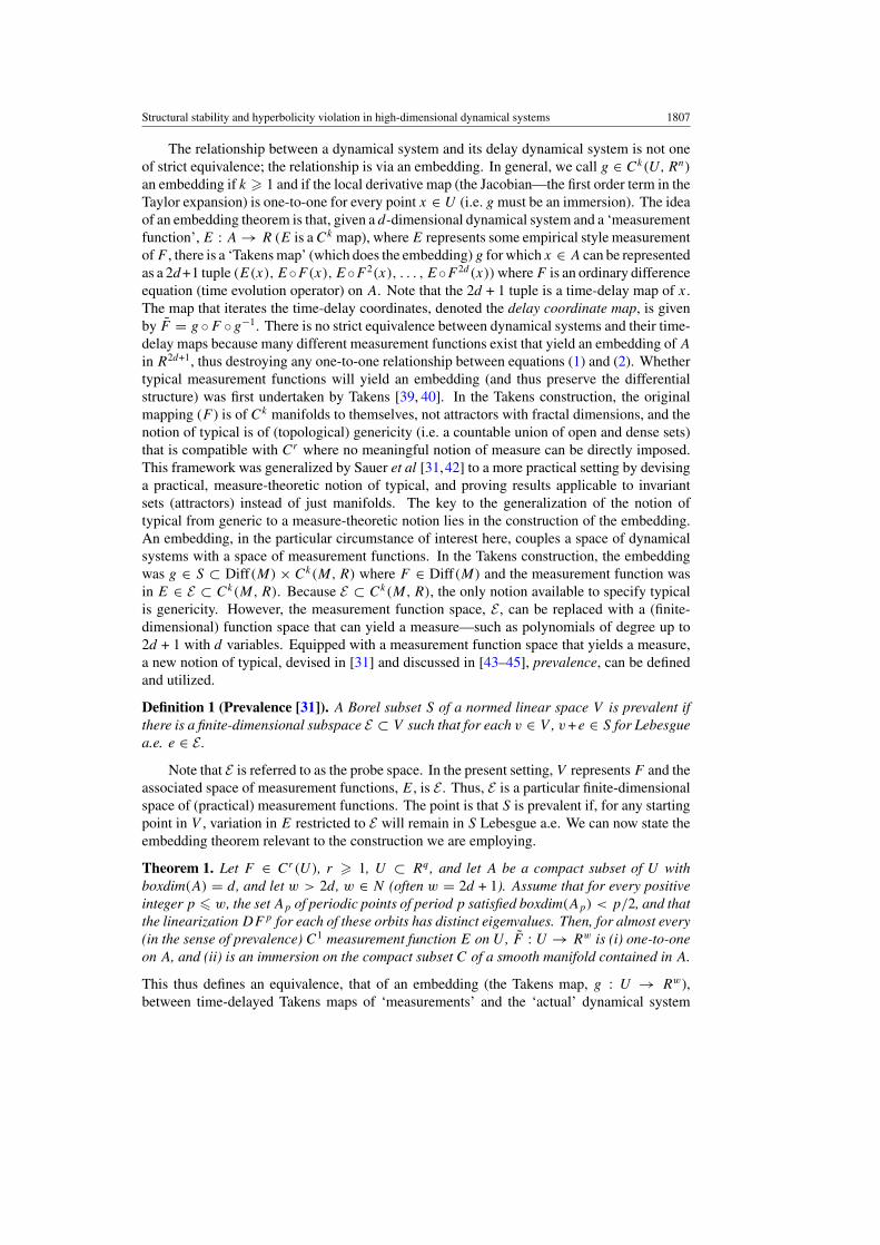
Figure 1. Schematic diagram of the embedding theorems applied to our construction.
operating in time on xt ∈ U . This does not imply that all time-delay maps can be embeddingsof a Cr dynamical system (see [31] for a detailed discussion of how time-delay dynamicalsystems can fail to yield an embedding).
To explicitly demonstrate how this applies to our circumstances, consider figure 1 in whichF and E are as given above and the embedding g is explicitly given by
g(xt ) = (E(xt ), E(F (xt )), . . . , E(F 2d(xt ))). (3)
In a colloquial, experimental sense, F just keeps track of the observations from themeasurement functionE and, at each time step, shifts the newest observation into thew = 2d+1tuple and sequentially shifts the scalar observation at time t (yt ) of the 2d + 1 tuple to the t − 1position of the 2d + 1 tuple. In more explicit notation, F is the following mapping:
(y1, . . . , y2d+1) → (y2, . . . , y2d+1, g(F (g−1(y1, . . . , y2d+1)))), (4)
where, again, F = g ◦ F ◦ g−1. The embedology theorem of Sauer et al says that there isa prevalent Borel subset (in a probe space, S) of measurement functions (E) of dynamicalsystems of the form (1) (F ), which will yield an embedding g of A. The neural networks wewill propose in the sections that follow can approximate F and its derivatives (to any order)to arbitrary accuracy (a notion we will make more precise later). Thus, we will investigate thespace of Cr dynamical systems given by (1) via the mappings used to approximate them.
2.1.2. Abstract neural networks. Begin by noting that, in general, a feed-forward, scalarneural network is a Cr mapping γ : Rd → R; the set of feed-forward, scalar networks with asingle hidden layer, �(G), can be written as:
�(G) ≡ {γ : Rd → R|γ (x) =N∑
i=1
βiG(xT ωi)}, (5)
where x ∈ Rd is the d-vector of network inputs, xT ≡ (1, xT ) (where xT is the transposeof x), N is the number of hidden units (neurons), β1, . . . , βN ∈ R are the hidden-to-outputlayer weights, ω1, . . . , ωN ∈ Rd+1 are the input-to-hidden layer weights and G : Rd → R is
Structural stability and hyperbolicity violation in high-dimensional dynamical systems 1809
the hidden layer activation function (or neuron). The partial derivatives of the network outputfunction, γ , are
∂γ (x)
∂xk
=N∑
i=1
βiωikDG(xT ωi), (6)
where xk is the kth component of the x vector, ωik is the kth component of ωi and DG is theusual first derivative of G. The matrix of partial derivatives (the Jacobian) takes a particularlysimple form when the x vector is a sequence of time delays (xt = (yt , yt−1, . . . , yt−(d−1)) forxt ∈ Rd and yi ∈ R). It is precisely for this reason that the time-delayed formulation easesthe computational woes.
This paper contains numerical evidence of a geometric mechanism, specified by theLyapunov spectrum, that is present in the above class of functions as d → ∞. In doingso, we will often make arguments that involve taking d → ∞ while leaving N limits vague.That we can do this is a result of the function approximation characteristics of the neuralnetworks; to see N specified in particular see [34, 46].
2.1.3. Neural networks as function approximations. Hornik et al [30] provided the theoreticaljustification for the use of neural networks as function approximators. The aforementionedauthors provide a degree of generality that we will not need; for their results in full generalitysee [30, 47].
The ability of neural networks to approximate (and be dense in) the space of mappingsrelevant to dynamics is the subject of the keynote theorems of Hornik et al [30] (for their resultsin full generality see [30, 47]). However, to state these theorems, a discussion of Sobolevfunction space, Sm
p , is required. We will be brief, noting references Adams and Fourier [48]and Hebey [49] for readers wanting more depth with respect to Sobolev spaces. For the sakeof clarity and simplification, let us make a few remarks which will pertain to the rest of thissection:
(i) µ is a measure; λ is the standard Lebesgue measure; for all practical purposes, µ = λ;(ii) l, m and d are finite, non-negative integers; m will be with reference to a degree of
continuity of some function spaces and d will be the dimension of the space we areoperating on;
(iii) p ∈ R, 1 � p < ∞; p will be with reference to a norm—either the Lp norm or theSobolev norm;
(iv) U ⊂ Rd , U is measurable.(v) α = (α1, α2, . . . , αd)
T is a d-tuple of non-negative integers (or a multi-index) satisfying|α| = α1 + α2 + · · · + αk , |α| � m;
(vi) for x ∈ Rd , xα ≡ xα11 · x
α22 , . . . , x
αd
d ;(vii) Dα denotes the partial derivative of order |α|
∂ |α|
∂xα≡ ∂ |α|
(∂xα11 ∂x
α22 . . . ∂x
αd
d ); (7)
(viii) u ∈ L1loc(U) is a locally integrable, real valued function on U ;
(ix) ρmp,µ is a metric, dependent on the subset U , the measure µ, and p and m in a manner we
will define shortly;(x) ‖ · ‖p is the standard norm in Lp(U);
1810 D J Albers and J C Sprott
Letting m be a positive integer and 1 � p < ∞, we define the Sobolev norm, ‖ · ‖m,p, asfollows:
||u||m,p = ∑
0�|α|�m
(‖ Dαu ‖pp)
1/p
, (8)
where u ∈ L1loc(U) is a locally integrable, real valued function on U ⊂ Rd (u could be
significantly more general) and || · ||p is the standard norm in Lp(U). Likewise, the Sobolevmetric can be defined:
ρmp,µ(f, g) ≡ ||f − g||m,p,U,µ. (9)
It is important to note that this metric is dependent on U .For ease of notation, let us define the set of m-times differentiable functions on U ,
Cm(U) = {f ∈ C(U)|Dαf ∈ C(U), ||Dαf ||p < ∞ ∀α, |α| � m}. (10)
We are now free to define the Sobolev space for which our results will apply.
Definition 2. For any positive integer m and 1 � p < ∞, we define a Sobolev space Smp (U, λ)
as the vector space on which || · ||m,p is a norm:
Smp (U, λ) = {f ∈ Cm(U)| ||Dαf ||p,U,λ < ∞ for all |α| � m} (11)
Equipped with the Sobolev norm, Smp is a Sobolev space over U ⊂ Rd .
Two functions in Smp (U, λ) are close in the Sobolev metric if all the derivatives of order
0 � |α| < m are close in the Lp metric. It is useful to recall that we are attempting toapproximate F = g ◦ F ◦ g−1 where F : R2d+1 → R; for this task the functions fromSm
p (U, λ) will serve quite nicely. The whole point of all this machinery is to state approximationtheorems that require specific notions of density. Otherwise we would refrain and instead usethe standard notion of Ck functions—the functions that are k-times differentiable uninhibitedby a notion of a metric or norm.
Armed with a specific function space for which the approximation results apply (thereare many more), we will conclude this section by briefly stating one of the approximationresults. However, before stating the approximation theorem, we need two definitions—onewhich makes the notion of closeness of derivatives more precise and one which gives thesufficient conditions for the activation functions to perform the approximations.
Definition 3 (m-uniformly dense). Assume m and l are non-negative integers 0 � m � l,U ⊂ Rd and S ⊂ Cl(U). If for any f ∈ S, compact K ⊂ U and ε > 0 there exists ag ∈ �(G) such that
max|α|�m
supx∈K
|Dαf (x) − Dαg(x)| < ε (12)
then �(G) is m-uniformly dense on compacta in S.
It is this notion of m-uniformly dense in S that provides all the approximation power of boththe mappings and the derivatives (up to order l) of the mappings. Next we will supply thecondition on our activation function necessary for the approximation results.
Definition 4 (l-finite). Let l be a non-negative integer. G is said to be l-finite for G ∈ Cl(R)
if
0 <
∫|DlG|dλ < ∞, (13)
i.e. the lth derivative of G must be both bounded away from zero, and finite for all l (recall dλ
is the standard Lebesgue volume element).
Structural stability and hyperbolicity violation in high-dimensional dynamical systems 1811
The hyperbolic tangent, our activation function, is l-finite.With these two notions, we can state one of the many existing approximation results.
Corollary 1. (corollary 3.5 [30] ) If G is l-finite, 0 � m � l, and U is an open subset of Rd ,then �(G) is m-uniformly dense on compacta in Sm
p (U, λ) for 1 � p < ∞.
In general, we wish to investigate differentiable mappings of compact sets to themselves.Further, we wish for the derivatives to be finite almost everywhere. Thus, the space Sm
p (U, λ)
will suffice for our purposes. Our results also apply to piecewise differentiable mappings.However, this requires a more general Sobolev space, Wm
p . We have refrained from delvinginto the definition of this space since it requires a bit more formalism. For those interestedsee [30] and [48].
2.1.4. Explicit neural network construction. The single layer feed-forward neural networks(γ from the above section) we will consider are of the form
xt = β0 +N∑
i=1
βiG
sωi0 + s
d∑j=1
ωijxt−j
, (14)
which is a map from Rd to R. The squashing function G, for our purpose, will be thehyperbolic tangent. In (14), N represents the number of hidden units or neurons, d is the inputor embedding dimension of the system which functions simply as the number of time lags ands is a scaling factor on the weights.
The parameters are real (βi, ωij , xj , s ∈ R) and the βi and ωij are elements ofweight matrices (which we hold fixed for each case). The initial conditions are denoted(x0, x1, . . . , xd), and (xt , xt+1, . . . , xt+d) represents the current state of the system at time t .The βs are iid uniform over [0, 1] and then re-scaled to satisfy the condition
∑Ni=1 β2
i = N .The ωij s are iid normal with zero mean and unit variance. The s parameter is a real numberand can be interpreted as the standard deviation of the w matrix of weights. The initial xj arechosen iid uniform on the interval [−1, 1]. All the weights and initial conditions are selectedrandomly using a pseudo-random number generator [50, 51].
We would like to make a few notes with respect to the squashing function, tanh(). First,tanh(x), for |x| 1, will tend to behave much like a binary function. Thus, the states of theneural network will tend towards the finite set (β0 ±β1 ±β2 . . .±βN), or a set of 2N differentstates. In the limit where the arguments of tanh() become infinite, the neural network willhave periodic dynamics. Thus, if 〈β〉 or s become very large, the system will have a greatlyreduced dynamic variability. Based on this problem, one might feel tempted to bound the β
a la∑N
i=1 |βi | = k fixing k for all N and d. This is a bad idea, however, since, if the βi arerestricted to a sphere of radius k, as N is increased, 〈βi
2〉 goes to zero [52]. The other extremeof tanh() also yields a very specific behaviour type. For x very near 0, the tanh(x) functionis nearly linear. Thus, choosing s small will force the dynamics to be mostly linear, againyielding fixed point and periodic behaviour (no chaos). Thus the scaling parameter s providesa unique bifurcation parameter that will sweep from linear ranges to highly non-linear ranges,to binary ranges—fixed points to chaos and back to periodic phenomena.
2.1.5. Neural network approximation theorems and the implicit measure. Because the neuralnetworks can be identified with points in Rk(k = N(d+2)+2), we impose a probability measureon �(tanh) by imposing a probability measure on parameter space Rk . These measures, whichwere explicitly defined in section 2.1.4, can be denoted mβ (on the β), mω (on the ω), ms
(on s), and mI (on the initial conditions) and form a product measure on Rk × Rd in the
1812 D J Albers and J C Sprott
standard way. All the results in this paper are subject to this measure—this is part of the pointof this construction. We are not studying a particular dynamical system, but rather we areperforming a statistical study of a function space. From the measure-theoretic perspective,all networks are represented with this measure, although clearly not with equal likelihood.For instance, Hamiltonian systems are likely a zero measure set relative to the measures weutilize. Moreover, the joint-probability distributions characteristic of neural networks, wheretraining has introduced correlations between weights, will likely produce greatly varying resultsdepending on the source of the training (for analytical tools for the analysis of trained networks,see [53]).
Specifying ‘typical’, or forging a connection between the results we present and the resultsof other computational studies, or the results from abstract dynamics is a delicate problem.Most abstract dynamics results are specified for the Cr function space in the Ck Whitneytopology using the notion of a residual (generic) subset because no sensible measure canbe imposed on the infinite-dimensional space of Cr systems. Because we are utilizing aspace that, with finitely many parameters, is a finite-dimensional approximation of Cr , thespace we study will always be non-residual relative to Cr . In fact, even when m-uniformaldensity is achieved at N = ∞, Cr still has an uncountably infinite number of dimensions asopposed to the countably infinite number of dimensions induced by m-uniformal density on�(tanh). Moreover, because we are studying a space of functions and not a particular mapping,comparing results of, say, coupled-map lattices with our study must be handled with great care.A full specification of such relationships, which we will only hint at here, will involve two keyaspects. First, the proper language to relate the finite-dimensional neural network constructionto the space of embeddings of dynamical systems is that of prevalence [43–45]. Prevalence(see definition 1) provides a measure-theoretic means of coping with the notion of typicalbetween finite and infinite-dimensional spaces. Second, training the neural networks induces(joint) probability measures on the weight structure and thus a means of comparison in measureof various different qualitative dynamics types (see [53] as a starting point). In the simplestsituation, if the measures of two trained ensembles of networks are singular with respect toeach other, it is likely that the sets containing the volume as determined by the measures aredisjoint. Thus, the space, �(tanh), with different measures can be used to quantify, in a preciseway, the relationship between different dynamical types.
In a practical sense, this construction is easily extendible in various ways. One extension ofparticular relevance involves imposing different measures on each component of Rk producinga more non-uniform connection structure between the states (a different network structure).Another extension involves imposing a measure via training [41, 54, 55] on, for instance,coupled-map data (or data from any other common mapping). Because the latter situationinduces a dependence between the weights, thus Rk will be equipped with a joint probabilitymeasure rather than a simple product measure. Given the neural network approximationtheorems, imposing different measures, and in particular, correlations between the weights,should have the same effect that studying different physical systems will have. The point is,with the abstract framework outlined above, there is a way of classifying and relating systemsby their dynamics via the space of measures on the parameter space of neural networks.
2.2. Characteristic Lyapunov exponents, hyperbolicity, and structural stability
The theories of hyperbolicity, Lyapunov exponents and structural stability have had a long,wonderful and tangled history beginning with Smale [56] (for other good starting pointssee [9,11,13,57]). We will, of course, only scratch the surface with our current discussion, butrather put forth the connections relevant for our work. In structural stability theory, topological
Structural stability and hyperbolicity violation in high-dimensional dynamical systems 1813
equivalence is the notion of equivalence between dynamical systems, and structural stabilityis the notion of the persistence of topological structure.
Definition 5 (Structural stability). A Cr discrete-time map, f , is structurally stable if thereis a Cr neighbourhood, V of f , such that any g ∈ V is topologically conjugate to f , i.e. forevery g ∈ V , there exists a homeomorphism h such that f = h−1 ◦ g ◦ h.
In other words, a map is structurally stable if, for all other maps g in a Cr neighbourhood, thereexists a homeomorphism that will map the domain of f to the domain of g, the range of f tothe range of g and the inverses, respectively. Structural stability is a purely topological notion.The hope of Smale and others was that structural stability would be open-dense (generic) inthe space of Cr dynamical systems as previously noted in section 1.2 (see [1] for counter-examples). Palis and Smale then devised the stability conjecture that would fundamentally tietogether hyperbolicity and structural stability.
The most simple and intuitive definition of hyperbolic applies to the linear case.
Definition 6 (Hyperbolic linear map). A linear map of Rn is called hyperbolic if all of itseigenvalues have modulus different from one.
Because strict hyperbolicity is a bit restrictive, we will utilize the notion of uniform partialhyperbolicity which will make precise the notion of a ‘little bit’ of hyperbolicity.
Definition 7 (Partial hyperbolicity). The diffeomorphism f of a smooth Riemannianmanifold M is said to be partially hyperbolic if for all x ∈ M the tangent bundle TxM
has the invariant splitting:
TxM = Eu(x) ⊕ Ec(x) ⊕ Es(x) (15)
into strong stable Es(x) = Esf (x), strong unstable Eu(x) = Eu
f (x) and central Ec(x) =Ec
f (x) bundles, at least two of which are non-trivial6. Thus, there will exist numbers0 < a < b < 1 < c < d such that, for all x ∈ M:
v ∈ Eu(x) ⇒ d||v|| � ||Dxf (v)||, (16)
v ∈ Ec(x) ⇒ b||v|| � ||Dxf (v)|| � c||v||, (17)
v ∈ Es(x) ⇒ ||Dxf (v)|| � a||v||. (18)
There are other definitions of hyperbolicity and related quantities such as non-uniform partialhyperbolicity and dominated splittings; more specific characteristics and definitions can befound in [7, 19, 20, 58, 59]. The key provided by definition 7 is the allowance of centrebundles, zero Lyapunov exponents and, in general, neutral directions, which are not allowed instrict hyperbolicity. Thus, we are allowed to keep the general framework of good topologicalstructure, but we lose structural stability. With non-trivial partial hyperbolicity (i.e. Ec is notnull), stable ergodicity replaces structural stability as the notion of dynamic stability in thePugh–Shub stability conjecture (conjecture (5) of [60]). Thus, what is left is to again attemptto show the extent to which stable ergodicity persists.
In numerical simulations we will never observe an orbit on the unstable, stable or centremanifolds (or the bundles). Thus, we will need a global notion of stability averaged along agiven orbit (which will exist under weak ergodic assumptions). The notion we seek is capturedby the spectrum of Lyapunov exponents.
6 If Ec is trivial, f is simply Anosov, or strictly hyperbolic.
1814 D J Albers and J C Sprott
Definition 8 (Lyapunov Exponents). Let f : M → M be a diffeomorphism (i.e. discretetime map) on a compact Riemannian manifold of dimension m. Let | · | be the norm on thetangent vectors induced by the Riemannian metric on M . For every x ∈ M and v ∈ TxM
Lyapunov exponent at x is denoted:
χ(x, v) = lim supt→∞
1
tlog ||Df nv||. (19)
Assume the function χ(x, ·) has only finitely many values on TxM {0} (this assumption may notbe true for our dynamical systems) which we denote χ
f
1 (x) < χf
2 (x) . . . < χfm(x). Next denote
the filtration of TxM associated with χ(x, ·), {0} = V0(x) � V1(x) � . . . � Vm(x) = TxM ,where Vi(x) = {v ∈ TxM|χ(x, v) � χi(x)}. The number ki = dim(Vi(x))− dim(Vi−1(x)) isthe multiplicity of the exponent χi(x). In general, for our networks over the parameter rangewe are considering, ki = 1 for all 0 < i � m. Given the above, the Lyapunov spectrum for f
at x is defined as:
Spχ(x) = {χkj (x)|1 � i � m}. (20)
(For more information regarding Lyapunov exponents and spectra see [61–64]).A more computationally motivated formula for the Lyapunov exponents is given as
χj = limN→∞
1
N
N∑k=1
ln(〈(Dfk · δxj )T , (Dfk · δxj )〉) (21)
where 〈, 〉 is the standard inner product, δxj is the j th component of the x variation7 andDfk is the ‘orthogonalized’ Jacobian of f at the kth iterate of f (x). Through the course ofour discussions we will dissect equation (21) further. It should also be noted that Lyapunovexponents have been shown to be independent of coordinate system. Thus, the specifics of ourabove definition do not affect the outcome of the exponents.
For the systems we study, there could be an x dependence on equations (19) and (21). Aswill be seen in later sections, we do not observe much of an x-dependence on the Lyapunovexponents over the parameter ranges considered. The existence (or lack) of multiple attractorshas been partially addressed in a conjecture in [65]; however, a more systematic study iscurrently under way.
In general, the existence of Lyapunov exponents is established by a multiplicative ergodictheorem (for a nice example, see theorem (1.6) in [66]). There exist many such theoremsfor various circumstances. The first multiplicative ergodic theorem was proved by Oseledec[67]; many others—[20, 68–72]—have subsequently generalized his original result. We willrefrain from stating a specific multiplicative ergodic theorem; the conditions necessary for theexistence of Lyapunov exponents are exactly the conditions we place on our function spacein section 2.3, that is, a Cr (r > 0) map of a compact manifold M (or open set U ) to itselfand an f -invariant probability measure ρ, on M (or U ). For specific treatments we leave thecurious reader to study the aforementioned references, noting that our construction followsfrom [20, 59, 69].
There is an intimate relationship between Lyapunov exponents and global stable andunstable manifolds. In fact, each Lyapunov exponent corresponds to a global manifold,and often the existence of the various global manifolds is explicitly tied to the existenceof the respective Lyapunov exponents. We will be using the global manifold structure asour measure of topological equivalence and the Lyapunov exponents to classify this globalstructure. Positive Lyapunov exponents correspond to global unstable manifolds, and negativeLyapunov exponents correspond to global stable manifolds. We will again refrain from stating
7 In a practical sense, the x variation is the initial separation or perturbation of x.
Structural stability and hyperbolicity violation in high-dimensional dynamical systems 1815
the existence theorems for these global manifolds (see [64] for a good discussion of this) andinstead note that in addition to the requirements for the existence of Lyapunov exponents, theexistence of global stable/unstable manifolds corresponding to the negative/positive Lyapunovexponents requires Df to be injective. For specific global unstable/stable manifold theoremssee [69].
Finally, the current best solution to the structural stability conjecture of Palis andSmale, the result that links hyperbolicity to structural stability, is captured in the followingtheorem.
Theorem 2 (Mane [5] theorem A, Robbin [3], Robinson [73]). A C1 diffeomorphism (on acompact, boundaryless manifold) is structurally stable if and only if it satisfies axiom A andthe strong transversality condition.
Recall that axiom A says the diffeomorphism is hyperbolic with dense periodic points onits non-wandering set � (p ∈ � is non-wandering if for any neighbourhood U of x, thereis an n > 0 such that f n(U) ∩ U �= 0). We will save a further explicit discussion of thisinterrelationship for a later section, noting that much of this report investigates the abovenotions and how they apply to our set of maps. Finally, for a nice, sophisticated introductionto the above topics see [62] or [74].
2.3. Conditions needed for the existence and computation of Lyapunov exponents
We will follow the standard constructions for the existence and computation of Lyapunovexponents as defined by the theories of Katok [68], Ruelle [66, 69], Pesin [70–72], Brin andPesin [20] and Burns et al [59].
Let H be a separable real Hilbert space (for practical purposes Rn) and let X be an opensubset of H. Next let (X, �, ρ) be a probability space where � is a σ -algebra of sets andρ is a probability measure, ρ(X) = 1 (see [75] for more information). Now consider a Cr
(r > 1) map ft : X → X which preserves ρ (ρ is f -invariant, at least on the unstablemanifolds) defined for t � T0 � 0 such that ft1+t2 = ft1 ◦ ft2 and that (x, t) → ft (x), Dft(x)
is continuous from X × [T0, ∞) to X and bounded on H. Assume that f has a compactinvariant set
� ={ ⋂
t>T0
ft (X)|ft (�) ⊆ �
}(22)
and Dft is a compact bounded operator for x ∈ �, t > T0. Finally, endow ft with a scalarparameter s ∈ [0 : ∞]. This gives us the space (a metric space—the metric will be definedheuristically in section 2.1.4) of one parameter, Cr measure-preserving maps from boundedcompact sets to themselves with bounded first derivatives. It is for a space of the abovemappings that Ruelle shows the existence of Lyapunov exponents [69]; similar requirementsare made by Brin and Pesin [20] in a slightly more general setting. The systems we willstudy are dissipative dynamical systems, and thus area-contracting, so ρ will not be absolutelycontinuous with respect to Lebesgue measure onX. However, to compute Lyapunov exponents,it is enough for there to exist invariant measures that are absolutely continuous with respect toLebesgue on the unstable manifolds [64, 76–78]. Thus, the Lyapunov exponents in the systemswe study are computed relative to SRB measures [64] that are assumed, but not proved, to existfor systems we study. Implications of invariant measures for dissipative dynamical systemssuch as those studied here can be found in [79].
We can take X in the above construction to be the Rd of section 2.1.1. The neuralnetworks we use map their domains to compact sets; moreover, because they are constructedas time-delays, their domains are also compact. Further, their derivatives are bounded up to
1816 D J Albers and J C Sprott
arbitrary order; although for our purposes, only the first order need be bounded. Because theneural networks are deterministic and bounded, there will exist an invariant set of some type.We are relegated to assuming the existence of SRB measures with which we can calculatethe Lyapunov exponents because proving the existence of SRB measures, even for relativelysimple dissipative dynamical systems, is non-trivial [80, 81]. Indeed, there remains muchwork to achieve a full understanding of Lyapunov exponents for general dissipative dynamicalsystems that are not absolutely continuous; for a current treatment see [61] or [64]. Thespecific measure theoretic properties of our networks (i.e. issues such as absolute continuity,uniform/non-uniform hyperbolicity, basin structures) is a topic of current investigation. Ingeneral, up to the accuracy, interval of initial conditions and dimension we are concerned within this paper, the networks observed do not have multiple attractors and thus have a singleinvariant measure. We will not prove this here and, in fact, know of counter-examples to theformer statement for some parameter settings.
2.4. Definitions for numerical arguments
Because we are conducting a numerical experiment, it is necessary to present notions thatallow us to test our conjectures numerically. We will begin with a notion of continuity. Theheart of continuity is based on the following idea: if a neighbourhood about a point in thedomain is shrunk, this implies a shrinking of a neighbourhood of the range. However, wedo not have infinitesimals at our disposal. Thus, our statements of numerical continuity willnecessarily have a statement regarding the limits of numerical resolution below which ourresults are uncertain.
Let us now begin with a definition of bounds on the domain and range:
Definition 9 (εnum). εnum is the numerical accuracy of a Lyapunov exponent, χj .
Definition 10 (δnum). δnum is the numerical accuracy of a given parameter under variation.
Now, with our εnum and δnum defined as our numerical limits in precision, let us definenumerical continuity of Lyapunov exponents.
Definition 11 (num-continuous Lyapunov exponents). Given a one parameter map f :R1 × Rd → Rd , f ∈ Cr , r > 0, for which characteristic exponents χj exist (a.e. withrespect to an SRB measure). The map f is said to have num-continuous Lyapunov exponentsat (µ, x) ∈ R1 × Rd if for εnum > 0 there exists a δnum > 0 such that if
|s − s ′| < δnum (23)
then
|χj (s) − χj (s′)| < εnum (24)
for s, s ′ ∈ R1, for all j ∈ N such that 0 < j � d.
Another useful definition related to continuity is that of a function being Lipschitz continuous.
Definition 12 (num-Lipschitz). Given a one parameter map f : R1 × Rd → Rd , f ∈ Cr ,r > 0, for which characteristic exponents χj exist (and are the same under all invariantmeasures), the map f is said to have num-Lipschitz Lyapunov exponents at (µ, x) ∈ R1 × Rd
if there exists a real constant 0 < kχjsuch that
|χj (s) − χj (s′)| < kχj
|s − s ′|. (25)
Structural stability and hyperbolicity violation in high-dimensional dynamical systems 1817
Further, if the constant kχj< 1, the Lyapunov exponent is said to be contracting8 on the
interval [s, s ′] for all s ′ such that |s − s ′| < δnum.
Note that neither of these definitions imply strict continuity, but rather they provide boundson the difference between the change in parameter and the change in Lyapunov exponents.It is important to note that these notions are highly localized with respect to the domain inconsideration. We will not imply some sort of global continuity using the above definitions;rather, we will use these notions to imply that Lyapunov exponents will continuously (withinnumerical resolution) cross through zero upon parameter variation. We can never numericallyprove that Lyapunov exponents do not jump across zero, but for most computational exercises,a jump across zero that is below numerical precision is not relevant. This notion of continuitywill aid in arguments regarding the existence of periodic windows in parameter space.
Let us next define a Lyapunov exponent zero-crossing.
Definition 13 (Lyapunov exponent zero-crossing). A Lyapunov exponent zero-crossing issimply the point sχj
in parameter space such that a Lyapunov exponent continuously (ornum-continuously) crosses zero, e.g. for s − δ, χi > 0, and for s + δ, χi < 0.
For this report, a Lyapunov exponent zero-crossing is a transverse intersection with thereal line. For our networks non-transversal intersections of the Lyapunov exponents with thereal line certainly occur, but for the portion of parameter space we are investigating, they areextremely rare. Along the route-to-chaos for our networks, such non-transversal intersectionsare common, but we will save the discussion of that topic for a different report. Orbits forwhich the Lyapunov spectrum can be defined (in a numerical sense, Lyapunov exponents aredefined when they are convergent), yet at least one of the exponents is zero, are called non-trivially num-partially hyperbolic. We must be careful making statements with respect to theexistence of zero Lyapunov exponents implying the existence of centre manifolds Ec becausezero exponents may not correspond to a manifold.
Lastly, we define a notion of denseness for a numerical context. There are several waysof achieving such a notion—we will use the notion of a dense sequence.
Definition 14 (ε-dense). Given an ε > 0, an open interval (a, b) ⊂ R, and a sequence{c1, . . . , cn}, {c1, . . . , cn} is ε-dense in (a, b) if there exists an n such that for any x ∈ (a, b),there is an i, 1 � i < n, such that dist(x, ci) < ε.
In reality however, we will be interested in a sequence of sequences that are ‘increasingly’ε-dense in an interval (a, b). In other words, for the sequence of sequences
c11, · · · , c1
n1
c21, · · · , c2
n2
......
...
where ni+1 > ni (i.e. for a sequence of sequences with increasing cardinality), the subsequentsequences for increasing ni become a closer approximation of an ε-dense sequence.
Definition 15 (Asymptotically dense (a-dense)). A sequence Sj = {cj
1, . . . , cjnj
} ⊂ (a, b) offinite subsets is asymptotically dense in (a, b), if for any ε > 0, there is an N such that Sj isε-dense if j � N .
8 Note, there is an important difference between the Lyapunov exponent contracting, which implies some sort ofconvergence to a particular value, versus a negative Lyapunov exponent that implies a contracting direction on themanifold or in phase space.
1818 D J Albers and J C Sprott
For an intuitive example of this, consider a sequence S of k numbers where qk ∈ S, qk ∈ (0, 1).Now increase the cardinality of the set, spreading elements in such a way that they are uniformlydistributed over the interval. Density is achieved with the cardinality of infinity, but clearly,with a finite but arbitrarily large number of elements, we can achieve any approximation to adense set that we wish. There are, of course, many ways we can have a countably infinite setthat is not dense, and, as we are working with numerics, we must concern ourselves with howwe will approach this asymptotic density. We now need a clear understanding of when thisdefinition will apply to a given set. There are many pitfalls; for instance, we wish to avoidsequences such as (1, 1
2 , 13 , . . . , 1
n, . . .). We will, in the section that addresses a-density, state
the necessary conditions for an a-dense set for our purposes.
3. Conjectures
The point of this exercise is to begin to specify, in a computational framework, the variationin Lyapunov exponents and hyperbolicity in a space of high-dimensional dynamical systems.To achieve this goal, we will make four statements or conjectures that we will subsequentlysupport with numerical evidence. To begin, let us specify a condition that will be very valuableto the formulation of our ideas.
Condition 1. Given a map (neural network) as defined in section 2.1.4, if the parameter s ∈ R1
is varied num-continuously, then the Lyapunov exponents vary num-continuously.
Since there are many counterexamples to this condition, many of our results rely upon ourability to show how generally this condition applies in high-dimensional systems.
Definition 16 (Chain link set). Assume f is a mapping (neural network) as defined in section2.1.4. A chain link set is denoted as
V = {s ∈ R | χj (s) �= 0 for all 0 < j � d and χj (s) > 0 for some j > 0}.If χj (s) is continuous at its Lyapunov exponent zero-crossing, as we will show later (condition(1)), then V is open. Next, let Ck be a connected component of the closure of V , V . It can beshown that Ck ∩ V is a union of disjoint, adjacent open intervals of the form
⋃i (ai, ai+1).
Definition 17 (Bifurcation link set). Assume f is a mapping (neural network) as defined insection 2.1.4. Denote a bifurcation link set of Ck ∩ V as
Vi = (ai, ai+1). (26)
Assume the number of positive Lyapunov exponents for each Vi ⊂ V remains constant. If,upon a monotonically increasing variation in the parameter s, the number of positive Lyapunovexponents for Vi is greater than the number of positive Lyapunov exponents for Vi+1, V is saidto be LCE decreasing. Specifically, the endpoints of the Vi are the points where there existLyapunov exponent zero crossings. We are not particularly interested in these sets; however,we are interested in the collection of endpoints adjoining these sets.
Definition 18 (Bifurcation chain subset). Let V be a chain link set, and Ck a connectedcomponent of V . A bifurcation chain subset of Ck ∩ V is denoted as
Uk = {ai} (27)
or equivalently
Uk = ∂(Ck ∩ V ). (28)
Structural stability and hyperbolicity violation in high-dimensional dynamical systems 1819
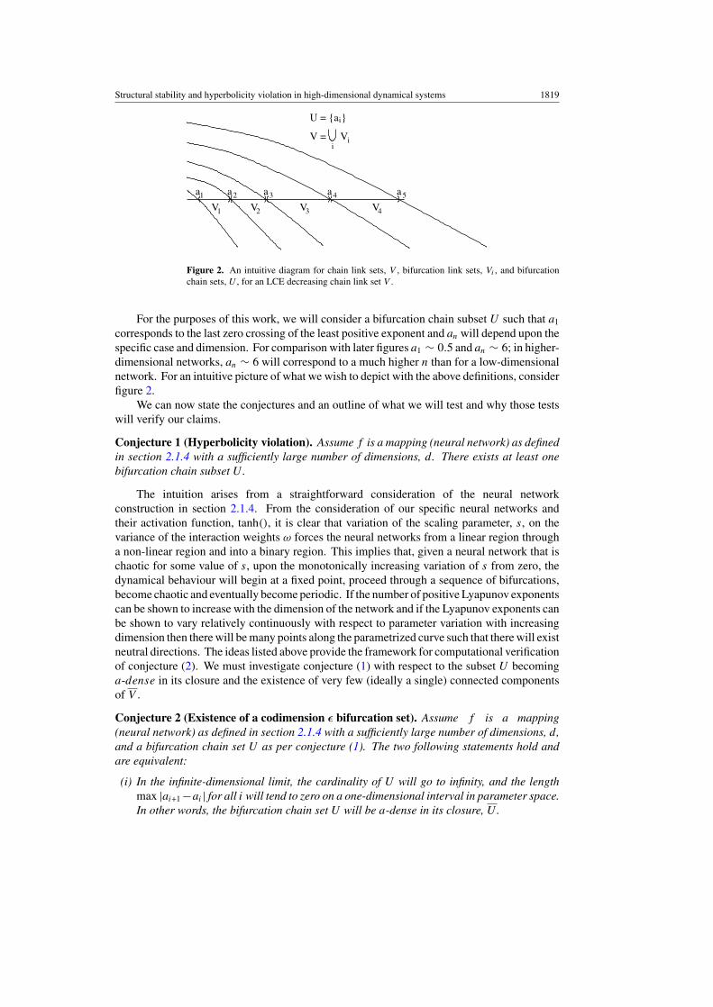
Figure 2. An intuitive diagram for chain link sets, V , bifurcation link sets, Vi , and bifurcationchain sets, U , for an LCE decreasing chain link set V .
For the purposes of this work, we will consider a bifurcation chain subset U such that a1
corresponds to the last zero crossing of the least positive exponent and an will depend upon thespecific case and dimension. For comparison with later figures a1 ∼ 0.5 and an ∼ 6; in higher-dimensional networks, an ∼ 6 will correspond to a much higher n than for a low-dimensionalnetwork. For an intuitive picture of what we wish to depict with the above definitions, considerfigure 2.
We can now state the conjectures and an outline of what we will test and why those testswill verify our claims.
Conjecture 1 (Hyperbolicity violation). Assume f is a mapping (neural network) as definedin section 2.1.4 with a sufficiently large number of dimensions, d. There exists at least onebifurcation chain subset U .
The intuition arises from a straightforward consideration of the neural networkconstruction in section 2.1.4. From the consideration of our specific neural networks andtheir activation function, tanh(), it is clear that variation of the scaling parameter, s, on thevariance of the interaction weights ω forces the neural networks from a linear region througha non-linear region and into a binary region. This implies that, given a neural network that ischaotic for some value of s, upon the monotonically increasing variation of s from zero, thedynamical behaviour will begin at a fixed point, proceed through a sequence of bifurcations,become chaotic and eventually become periodic. If the number of positive Lyapunov exponentscan be shown to increase with the dimension of the network and if the Lyapunov exponents canbe shown to vary relatively continuously with respect to parameter variation with increasingdimension then there will be many points along the parametrized curve such that there will existneutral directions. The ideas listed above provide the framework for computational verificationof conjecture (2). We must investigate conjecture (1) with respect to the subset U becominga-dense in its closure and the existence of very few (ideally a single) connected componentsof V .
Conjecture 2 (Existence of a codimension ε bifurcation set). Assume f is a mapping(neural network) as defined in section 2.1.4 with a sufficiently large number of dimensions, d,and a bifurcation chain set U as per conjecture (1). The two following statements hold andare equivalent:
(i) In the infinite-dimensional limit, the cardinality of U will go to infinity, and the lengthmax |ai+1 −ai | for all i will tend to zero on a one-dimensional interval in parameter space.In other words, the bifurcation chain set U will be a-dense in its closure, U .
1820 D J Albers and J C Sprott
2
M
N
= N chaotic dynamics with dense LE zero crossings
~
~
p1
p3
M
= N – codim(N)=0
= O – codim(O)=1
O
N
p
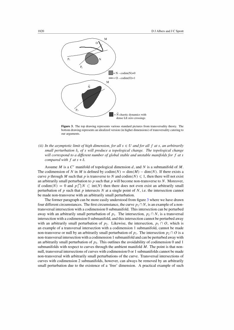
Figure 3. The top drawing represents various standard pictures from transversality theory. Thebottom drawing represents an idealized version (in higher dimensions) of transversality catering toour arguments.
(ii) In the asymptotic limit of high dimension, for all s ∈ U and for all f at s, an arbitrarilysmall perturbation δs of s will produce a topological change. The topological changewill correspond to a different number of global stable and unstable manifolds for f at s
compared with f at s + δ.
Assume M is a Cr manifold of topological dimension d, and N is a submanifold of M .The codimension of N in M is defined by codim(N) = dim(M) − dim(N). If there exists acurve p through M such that p is transverse to N and codim(N) � 1, then there will not existan arbitrarily small perturbation to p such that p will become non-transverse to N . Moreover,if codim(N) = 0 and p
⋂N ⊂ int(N) then there does not even exist an arbitrarily small
perturbation of p such that p intersects N at a single point of N , i.e. the intersection cannotbe made non-transverse with an arbitrarily small perturbation.
The former paragraph can be more easily understood from figure 3 where we have drawnfour different circumstances. The first circumstance, the curve p1 ∩N , is an example of a non-transversal intersection with a codimension 0 submanifold. This intersection can be perturbedaway with an arbitrarily small perturbation of p1. The intersection, p2 ∩ N , is a transversalintersection with a codimension 0 submanifold, and this intersection cannot be perturbed awaywith an arbitrarily small perturbation of p2. Likewise, the intersection, p1 ∩ O, which isan example of a transversal intersection with a codimension 1 submanifold, cannot be madenon-transverse or null by an arbitrarily small perturbation of p1. The intersection p2 ∩ O is anon-transversal intersection with a codimension 1 submanifold and can be perturbed away withan arbitrarily small perturbation of p2. This outlines the avoidability of codimension 0 and 1submanifolds with respect to curves through the ambient manifold M . The point is that non-null, transversal intersections of curves with codimension 0 or 1 submanifolds cannot be madenon-transversal with arbitrarily small perturbations of the curve. Transversal intersections ofcurves with codimension 2 submanifolds, however, can always be removed by an arbitrarilysmall perturbation due to the existence of a ‘free’ dimension. A practical example of such
Structural stability and hyperbolicity violation in high-dimensional dynamical systems 1821
would be the intersection of a curve with another curve in R3—one can always pull apart thetwo curves simply by ‘lifting’ them apart.
In the circumstance proposed in conjecture (2), the set U (N in figure 3) will always havecodimension d because U consists of finitely many points; thus, any intersection with U canbe removed by an arbitrarily small perturbation. The point is that, as U becomes a-dense inU , p3
⋂U = 0 becomes more and more unlikely, and the perturbations required to remove
the intersections of p3 with U (again, N as in figure 3 ) will become more and more bizarre.For a low-dimensional example, think of a ball of radius r in R3 that is populated by a finiteset of evenly distributed points, denoted Si , where i is the number of elements in Si . Next fita curve p through that ball in such a way that p does not hit any points in Si . Now, as thecardinality of Si becomes large, if Si is a-dense in the ball of radius r , for the intersection of p
with Si to remain null, p will need to become increasingly kinky. Moreover, continuous, lineartransformations of p will become increasingly unlikely to preserve p ∩ Si = 0. It is this typeof behaviour with respect to parameter variation that we are arguing for with conjecture (2).However, figure 3 should only be used as an tool for intuition—our conjectures are with respectto a particular interval in parameter space and not a general curve in parameter space, let alonea family of curves or a high-dimensional surface. Conjecture (2) is a first step towards a morecomplete argument with respect to the above scenario. For more information concerning theorigin of the above picture, see [82] or [83]. With the development of more mathematicallanguage, it is likely that this conjecture can be specified with the notion of prevalence.
To understand roughly why we believe conjecture (2) is reasonable, first take condition(1) for granted (we will expend some effort showing where condition (1) is reasonable).Next assume there are arbitrarily many Lyapunov exponents near 0 along some interval ofparameter space and that the Lyapunov exponent zero-crossings can be shown to be a-densewith increasing dimension. Further, assume that on the aforementioned interval, V is LCEdecreasing. Since varying the parameters continuously on some small interval will moveLyapunov exponents continuously, small changes in the parameters will guarantee a continualchange in the number of positive Lyapunov exponents. One might think of this intuitivelyrelative to the parameter space as the set of Lyapunov exponent zero-crossings forming acodimension 0 submanifold with respect to the particular interval of parameter space. However,we will never achieve such a situation in a rigorous way. Rather, we will have an a-densebifurcation chain set U , which will have codimension 1 in R with respect to topologicaldimension. As the dimension of f is increased, U will behave more like a codimension 0submanifold of R. Hence the metaphoric language, codimension ε bifurcation set. The set U
will always be a codimension one submanifold because it is a finite set of points. Nevertheless,if U tends towards being dense in its closure, it will behave increasingly like a codimensionzero submanifold. This argument will not work for the entirety of the parameter space, and thuswe will show where, to what extent, and under what conditions U exists and how it behavesas the dimension of the network is increased.
Conjecture 3 (Periodic window probability decreasing). Assume f is a mapping (neuralnetwork) as defined in section 2.1.4 and a bifurcation chain set U as per conjecture (1). Inthe asymptotic limit of high dimension, the length of the bifurcation chain sets, l = |an − a1|,increases such that the cardinality of U → m where m is the maximum number of positiveLyapunov exponents for f . In other words, there will exist an interval in parameter space (e.g.s ∈ (a1, an) ∼ (0.1, 4)) where the probability of the existence of a periodic window will go tozero (with respect to Lebesgue measure on the interval) as the dimension becomes large.
This conjecture is somewhat difficult to test for a specific function since adding inputscompletely changes the function. Thus, the curve through the function space is an abstraction
1822 D J Albers and J C Sprott
which is not afforded by our construction. We will save a more complete analysis (e.g. a searchfor periodic windows along a high-dimensional surface in parameter space) of conjecture (3)for a different report. In this work, conjecture (3) addresses a very practical matter, for it impliesthe existence of a much smaller number of bifurcation chain sets. The previous conjecturesallow for the existence of many of these bifurcation chains sets, U , separated by windows ofperiodicity in parameter space. However, if these windows of periodic dynamics in parameterspace vanish, we could end up with only one bifurcation chain set—the ideal situation for ourarguments. We will not claim such; however, we will claim that the length of the set U we areconcerning ourselves with in a practical sense will increase with increasing dimension, largelydue to the disappearance of periodic windows on the closure of V . With respect to this report,all that needs to be shown is that the window sizes along the path in parameter space for avariety of neural networks decreases with increasing dimension. From a qualitative analysis,it will be somewhat clear that the above conjecture is reasonable.
If this paper were actually making statements we could rigorously prove; conjectures (1),(2) and (3) would function as lemmas for conjecture (4).
Conjecture 4. Assume f is a mapping (neural network) as defined in section 2.1.4 with asufficiently large number of dimensions, d, a bifurcation chain set U as per conjecture (1) andthe chain link set V . The perturbation size δs of s ∈ Cmax , where Cmax is the largest connectedcomponent of V , for which f |Ck
remains structurally stable, goes to zero as d → ∞.
Specific cases and the lack of density of structural stability in certain sets of dynamicalsystems has been proved long ago. These examples were, however, very specialized andcarefully constructed circumstances and do not speak of the commonality of structural stabilityfailure. Along the road to investigating conjecture (4) we will show that structural stabilitywill not, in a practical sense, be observable for a large set of very high-dimensional dynamicalsystems along certain, important intervals in parameter space even though structural stabilityis a property that will exist on that interval with probability one (with respect to Lebesguemeasure). This conjecture might appear to contradict some well-known results in stabilitytheory. A careful analysis of this conjecture, and its relation to known results, will be discussedin sections 7.1.4 and 7.3.1.
The larger question that remains, however, is whether conjecture (4) is valid on high-dimensional surfaces in parameter space. We believe this is a much more difficult questionwith a much more complicated answer. A highly related problem of whether chaos persists inhigh-dimensional dynamical systems is partially addressed in [65].
4. Numerical errors and Lyapunov exponent calculation
The Lyapunov exponents are calculated by equation (21) using the well-known and standardtechniques given in [41, 84–86]. We employ the modified Gram–Schmidt orthogonalizationtechnique because it is more numerically stable than the standard Gram–Schmidt technique.Moreover, the orthonormalization is computed at every time step. The results are not alteredwhen we use other orthonormalization algorithms (see [87] for a survey of different techniques).The explicit calculation of LCEs in the context we utilize is discussed well in [88]. Numericalerror analysis for the Lypaunov exponent calculation has been studied in various contexts;see [89] or [90] for details. Determining errors in the Lyapunov exponents is not an exactscience; for our networks such errors vary a great deal in different regions in s space. Forinstance, near the first bifurcation from a fixed point can require up to 100 000 or more iterationsto converge to an attractor and 500 00 more iterations for the Lyapunov spectrum to converge.The region of parameter space we study here has particularly fast convergence.
Structural stability and hyperbolicity violation in high-dimensional dynamical systems 1823
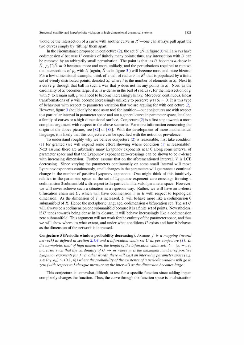
Figure 4. LE spectrum versus iteration for individual networks with 32 neurons and 16 (left, onlythe largest 8 are shown) and 64 (right) dimensions.
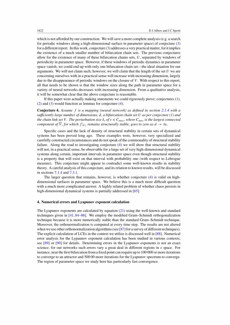
Figure 5. Close-up of LE spectrum versus iteration: 32 neurons, 64 dimensions.
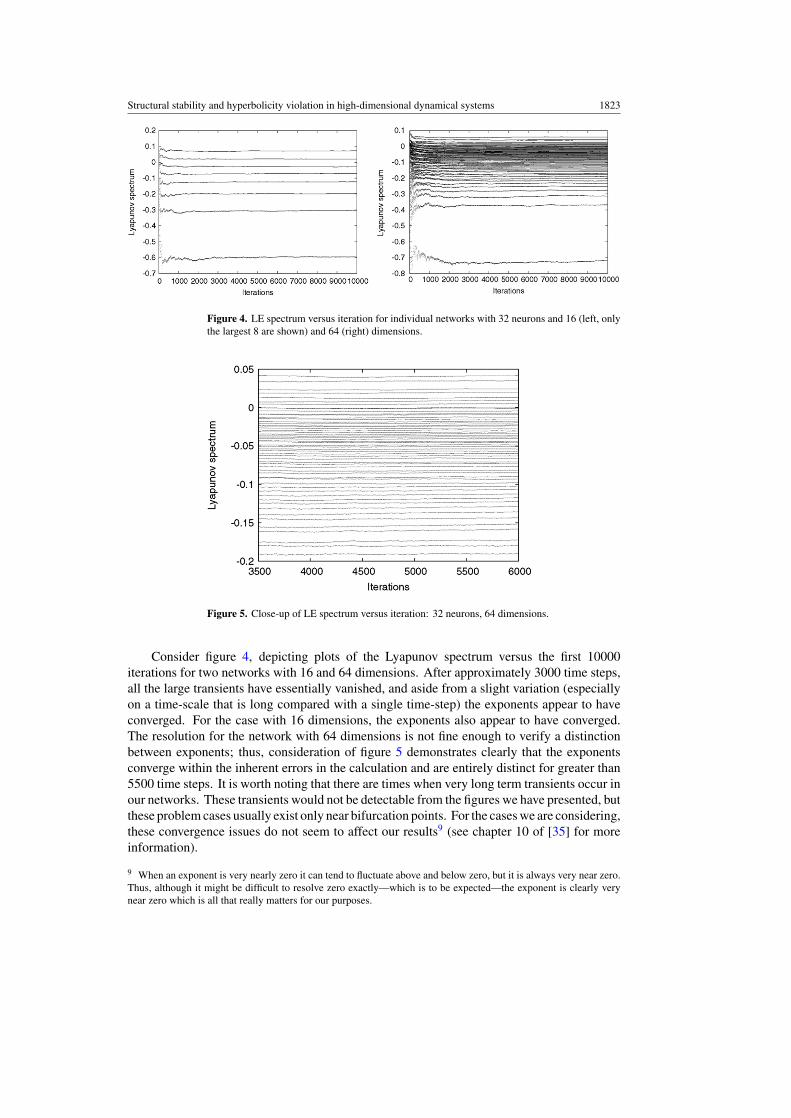
Consider figure 4, depicting plots of the Lyapunov spectrum versus the first 10000iterations for two networks with 16 and 64 dimensions. After approximately 3000 time steps,all the large transients have essentially vanished, and aside from a slight variation (especiallyon a time-scale that is long compared with a single time-step) the exponents appear to haveconverged. For the case with 16 dimensions, the exponents also appear to have converged.The resolution for the network with 64 dimensions is not fine enough to verify a distinctionbetween exponents; thus, consideration of figure 5 demonstrates clearly that the exponentsconverge within the inherent errors in the calculation and are entirely distinct for greater than5500 time steps. It is worth noting that there are times when very long term transients occur inour networks. These transients would not be detectable from the figures we have presented, butthese problem cases usually exist only near bifurcation points. For the cases we are considering,these convergence issues do not seem to affect our results9 (see chapter 10 of [35] for moreinformation).
9 When an exponent is very nearly zero it can tend to fluctuate above and below zero, but it is always very near zero.Thus, although it might be difficult to resolve zero exactly—which is to be expected—the exponent is clearly verynear zero which is all that really matters for our purposes.
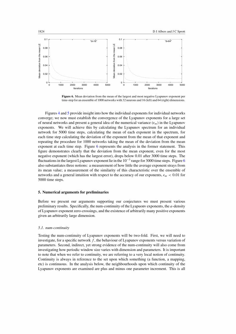
1824 D J Albers and J C Sprott
0
0.02
0.04
0.06
0.08
0.1
0 1000 2000 3000 4000 5000
Mea
n de
viat
ion
from
the
mea
n LE
Iterations
"d=16"
0
0.02
0.04
0.06
0.08
0.1
0 1000 2000 3000 4000 5000
Mea
n de
viat
ion
from
the
mea
n LE
Iterations
"d=64"
Figure 6. Mean deviation from the mean of the largest and most negative Lyapunov exponent pertime-step for an ensemble of 1000 networks with 32 neurons and 16 (left) and 64 (right) dimensions.
Figures 4 and 5 provide insight into how the individual exponents for individual networksconverge; we now must establish the convergence of the Lyapunov exponents for a large setof neural networks and present a general idea of the numerical variance (εm) in the Lyapunovexponents. We will achieve this by calculating the Lyapunov spectrum for an individualnetwork for 5000 time steps, calculating the mean of each exponent in the spectrum, foreach time step calculating the deviation of the exponent from the mean of that exponent andrepeating the procedure for 1000 networks taking the mean of the deviation from the meanexponent at each time step. Figure 6 represents the analysis in the former statement. Thisfigure demonstrates clearly that the deviation from the mean exponent, even for the mostnegative exponent (which has the largest error), drops below 0.01 after 3000 time steps. Thefluctuations in the largest Lyapunov exponent lie in the 10−3 range for 3000 time steps. Figure 6also substantiates three notions: a measurement of how little the average exponent strays fromits mean value; a measurement of the similarity of this characteristic over the ensemble ofnetworks and a general intuition with respect to the accuracy of our exponents, εm < 0.01 for5000 time steps.
5. Numerical arguments for preliminaries
Before we present our arguments supporting our conjectures we must present variouspreliminary results. Specifically, the num-continuity of the Lyapuonv exponents, the a-densityof Lyapunov exponent zero-crossings, and the existence of arbitrarily many positive exponentsgiven an arbitrarily large dimension.
5.1. num-continuity
Testing the num-continuity of Lyapunov exponents will be two-fold. First, we will need toinvestigate, for a specific network f , the behaviour of Lyapunov exponents versus variation ofparameters. Second, indirect, yet strong evidence of the num-continuity will also come frominvestigating how periodic window size varies with dimension and parameters. It is importantto note that when we refer to continuity, we are referring to a very local notion of continuity.Continuity is always in reference to the set upon which something (a function, a mapping,etc) is continuous. In the analysis below, the neighbourhoods upon which continuity of theLyapunov exponents are examined are plus and minus one parameter increment. This is all
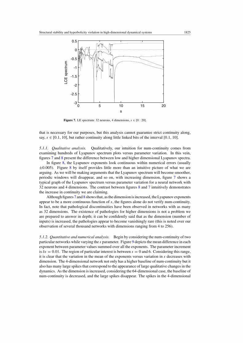
Structural stability and hyperbolicity violation in high-dimensional dynamical systems 1825
-3
-2.5
-2
-1.5
-1
-0.5
0
0.5
0 5 10 15 20
LCE
spe
ctru
m
s
Figure 7. LE spectrum: 32 neurons, 4 dimensions, s ∈ [0 : 20].
that is necessary for our purposes, but this analysis cannot guarantee strict continuity along,say, s ∈ [0.1, 10], but rather continuity along little linked bits of the interval [0.1, 10].
5.1.1. Qualitative analysis. Qualitatively, our intuition for num-continuity comes fromexamining hundreds of Lyapunov spectrum plots versus parameter variation. In this vein,figures 7 and 8 present the difference between low and higher dimensional Lyapunov spectra.
In figure 8, the Lyapunov exponents look continuous within numerical errors (usually±0.005). Figure 8 by itself provides little more than an intuitive picture of what we arearguing. As we will be making arguments that the Lyapunov spectrum will become smoother,periodic windows will disappear, and so on, with increasing dimension, figure 7 shows atypical graph of the Lyapunov spectrum versus parameter variation for a neural network with32 neurons and 4 dimensions. The contrast between figures 8 and 7 intuitively demonstratesthe increase in continuity we are claiming.
Although figures 7 and 8 shows that, as the dimension is increased, the Lyapunov exponentsappear to be a more continuous function of s, the figures alone do not verify num-continuity.In fact, note that pathological discontinuities have been observed in networks with as manyas 32 dimensions. The existence of pathologies for higher dimensions is not a problem weare prepared to answer in depth; it can be confidently said that as the dimension (number ofinputs) is increased, the pathologies appear to become vanishingly rare (this is noted over ourobservation of several thousand networks with dimensions ranging from 4 to 256).
5.1.2. Quantitative and numerical analysis. Begin by considering the num-continuity of twoparticular networks while varying the s parameter. Figure 9 depicts the mean difference in eachexponent between parameter values summed over all the exponents. The parameter incrementis δs = 0.01. The region of particular interest is between s = 0 and 6. Considering this range,it is clear that the variation in the mean of the exponents versus variation in s decreases withdimension. The 4-dimensional network not only has a higher baseline of num-continuity but italso has many large spikes that correspond to the appearance of large qualitative changes in thedynamics. As the dimension is increased, considering the 64-dimensional case, the baseline ofnum-continuity is decreased, and the large spikes disappear. The spikes in the 4-dimensional
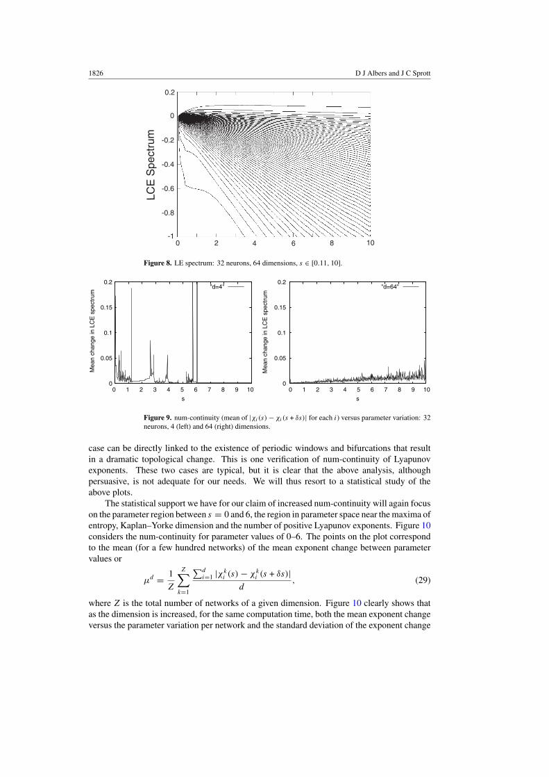
1826 D J Albers and J C Sprott
LCE
Spe
ctru
m
0 2 4 6 8 10-1
-0.8
-0.6
-0.4
-0.2
0
0.2
Figure 8. LE spectrum: 32 neurons, 64 dimensions, s ∈ [0.11, 10].
0
0.05
0.1
0.15
0.2
0 1 2 3 4 5 6 7 8 9 10
Mea
n ch
ange
in L
CE
spe
ctru
m
s
"d=4"
0
0.05
0.1
0.15
0.2
0 1 2 3 4 5 6 7 8 9 10
Mea
n ch
ange
in L
CE
spe
ctru
m
s
"d=64"
Figure 9. num-continuity (mean of |χi(s) − χi(s + δs)| for each i) versus parameter variation: 32neurons, 4 (left) and 64 (right) dimensions.
case can be directly linked to the existence of periodic windows and bifurcations that resultin a dramatic topological change. This is one verification of num-continuity of Lyapunovexponents. These two cases are typical, but it is clear that the above analysis, althoughpersuasive, is not adequate for our needs. We will thus resort to a statistical study of theabove plots.
The statistical support we have for our claim of increased num-continuity will again focuson the parameter region between s = 0 and 6, the region in parameter space near the maxima ofentropy, Kaplan–Yorke dimension and the number of positive Lyapunov exponents. Figure 10considers the num-continuity for parameter values of 0–6. The points on the plot correspondto the mean (for a few hundred networks) of the mean exponent change between parametervalues or
µd = 1
Z
Z∑k=1
∑di=1 |χk
i (s) − χki (s + δs)|
d, (29)
where Z is the total number of networks of a given dimension. Figure 10 clearly shows thatas the dimension is increased, for the same computation time, both the mean exponent changeversus the parameter variation per network and the standard deviation of the exponent change
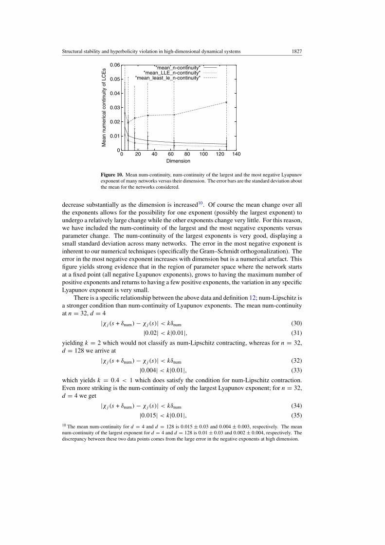
Structural stability and hyperbolicity violation in high-dimensional dynamical systems 1827
0
0.01
0.02
0.03
0.04
0.05
0.06
0 20 40 60 80 100 120 140
Mea
n nu
mer
ical
con
tinui
ty o
f LC
Es
Dimension
"mean_n-continuity""mean_LLE_n-continuity"
"mean_least_le_n-continuity"
Figure 10. Mean num-continuity, num-continuity of the largest and the most negative Lyapunovexponent of many networks versus their dimension. The error bars are the standard deviation aboutthe mean for the networks considered.
decrease substantially as the dimension is increased10. Of course the mean change over allthe exponents allows for the possibility for one exponent (possibly the largest exponent) toundergo a relatively large change while the other exponents change very little. For this reason,we have included the num-continuity of the largest and the most negative exponents versusparameter change. The num-continuity of the largest exponents is very good, displaying asmall standard deviation across many networks. The error in the most negative exponent isinherent to our numerical techniques (specifically the Gram–Schmidt orthogonalization). Theerror in the most negative exponent increases with dimension but is a numerical artefact. Thisfigure yields strong evidence that in the region of parameter space where the network startsat a fixed point (all negative Lyapunov exponents), grows to having the maximum number ofpositive exponents and returns to having a few positive exponents, the variation in any specificLyapunov exponent is very small.
There is a specific relationship between the above data and definition 12; num-Lipschitz isa stronger condition than num-continuity of Lyapunov exponents. The mean num-continuityat n = 32, d = 4
|χj (s + δnum) − χj (s)| < kδnum (30)
|0.02| < k|0.01|, (31)
yielding k = 2 which would not classify as num-Lipschitz contracting, whereas for n = 32,d = 128 we arrive at
|χj (s + δnum) − χj (s)| < kδnum (32)
|0.004| < k|0.01|, (33)
which yields k = 0.4 < 1 which does satisfy the condition for num-Lipschitz contraction.Even more striking is the num-continuity of only the largest Lyapunov exponent; for n = 32,d = 4 we get
|χj (s + δnum) − χj (s)| < kδnum (34)
|0.015| < k|0.01|, (35)10 The mean num-continuity for d = 4 and d = 128 is 0.015 ± 0.03 and 0.004 ± 0.003, respectively. The meannum-continuity of the largest exponent for d = 4 and d = 128 is 0.01 ± 0.03 and 0.002 ± 0.004, respectively. Thediscrepancy between these two data points comes from the large error in the negative exponents at high dimension.
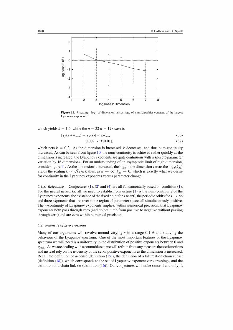
1828 D J Albers and J C Sprott
-4
-3
-2
-1
0
1
2
1 2 3 4 5 6 7 8
log
base
2 o
f k
log base 2 Dimension
Figure 11. k-scaling: log2 of dimension versus log2 of num-Lipschitz constant of the largestLyapunov exponent.
which yields k = 1.5, while the n = 32 d = 128 case is
|χj (s + δnum) − χj (s)| < kδnum (36)
|0.002| < k|0.01|, (37)
which nets k = 0.2. As the dimension is increased, k decreases; and thus num-continuityincreases. As can be seen from figure 10, the num-continuity is achieved rather quickly as thedimension is increased; the Lyapunov exponents are quite continuous with respect to parametervariation by 16 dimensions. For an understanding of an asymptotic limit of high dimension,consider figure 11. As the dimension is increased, the log2 of the dimension versus the log2(kχ1)
yields the scaling k ∼ √(2/d); thus, as d → ∞, kχ1 → 0, which is exactly what we desire
for continuity in the Lyapunov exponents versus parameter change.
5.1.3. Relevance. Conjectures (1), (2) and (4) are all fundamentally based on condition (1).For the neural networks, all we need to establish conjecture (1) is the num-continuity of theLyapunov exponents, the existence of the fixed point for s near 0, the periodic orbits for s → ∞and three exponents that are, over some region of parameter space, all simultaneously positive.The n-continuity of Lyapunov exponents implies, within numerical precision, that Lyapunovexponents both pass through zero (and do not jump from positive to negative without passingthrough zero) and are zero within numerical precision.
5.2. a-density of zero crossings
Many of our arguments will revolve around varying s in a range 0.1–6 and studying thebehaviour of the Lyapunov spectrum. One of the most important features of the Lyapunovspectrum we will need is a uniformity in the distribution of positive exponents between 0 andχmax. As we are dealing with a countable set, we will refrain from any measure theoretic notionsand instead rely on the a-density of the set of positive exponents as the dimension is increased.Recall the definition of a-dense (definition (15)), the definition of a bifurcation chain subset(definition (18)), which corresponds to the set of Lyapunov exponent zero crossings, and thedefinition of a chain link set (definition (16)). Our conjectures will make sense if and only if,
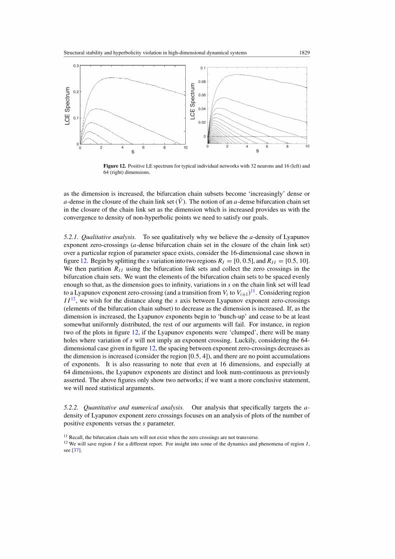
Structural stability and hyperbolicity violation in high-dimensional dynamical systems 1829
s
LCE
Spe
ctru
m
0 2 4 6 00
0.1
0.2
0.3
s
LCE
Spe
ctru
m
0
0.02
0.04
0.08
0.1
0 2 4 6 8 10
0.06
Figure 12. Positive LE spectrum for typical individual networks with 32 neurons and 16 (left) and64 (right) dimensions.
as the dimension is increased, the bifurcation chain subsets become ‘increasingly’ dense ora-dense in the closure of the chain link set (V ). The notion of an a-dense bifurcation chain setin the closure of the chain link set as the dimension which is increased provides us with theconvergence to density of non-hyperbolic points we need to satisfy our goals.
5.2.1. Qualitative analysis. To see qualitatively why we believe the a-density of Lyapunovexponent zero-crossings (a-dense bifurcation chain set in the closure of the chain link set)over a particular region of parameter space exists, consider the 16-dimensional case shown infigure 12. Begin by splitting the s variation into two regions RI = [0, 0.5], and RII = [0.5, 10].We then partition RII using the bifurcation link sets and collect the zero crossings in thebifurcation chain sets. We want the elements of the bifurcation chain sets to be spaced evenlyenough so that, as the dimension goes to infinity, variations in s on the chain link set will leadto a Lyapunov exponent zero-crossing (and a transition from Vi to Vi±1)11. Considering regionII 12, we wish for the distance along the s axis between Lyapunov exponent zero-crossings(elements of the bifurcation chain subset) to decrease as the dimension is increased. If, as thedimension is increased, the Lyapunov exponents begin to ‘bunch-up’ and cease to be at leastsomewhat uniformly distributed, the rest of our arguments will fail. For instance, in regiontwo of the plots in figure 12, if the Lyapunov exponents were ‘clumped’, there will be manyholes where variation of s will not imply an exponent crossing. Luckily, considering the 64-dimensional case given in figure 12, the spacing between exponent zero-crossings decreases asthe dimension is increased (consider the region [0.5, 4]), and there are no point accumulationsof exponents. It is also reassuring to note that even at 16 dimensions, and especially at64 dimensions, the Lyapunov exponents are distinct and look num-continuous as previouslyasserted. The above figures only show two networks; if we want a more conclusive statement,we will need statistical arguments.
5.2.2. Quantitative and numerical analysis. Our analysis that specifically targets the a-density of Lyapunov exponent zero crossings focuses on an analysis of plots of the number ofpositive exponents versus the s parameter.
11 Recall, the bifurcation chain sets will not exist when the zero crossings are not transverse.12 We will save region I for a different report. For insight into some of the dynamics and phenomena of region I ,see [37].
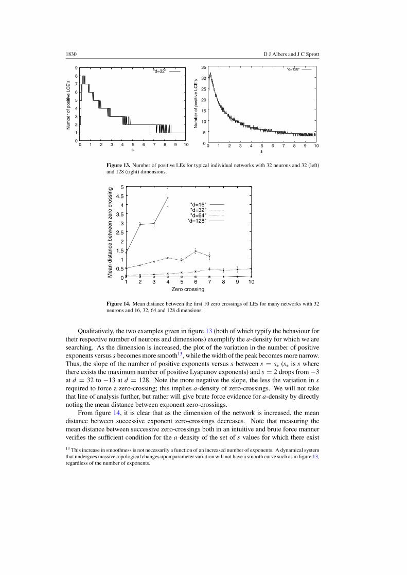
1830 D J Albers and J C Sprott
0
1
2
3
4
5
6
7
8
9
0 1 2 3 4 5 6 7 8 9 10
Num
ber
of p
ositi
ve L
CE
’s
Num
ber
of p
ositi
ve L
CE
’s
s
"d=32"
0
5
10
15
20
25
30
35
0 1 2 3 4 5 6 7 8 9 10s
"d=128"
Figure 13. Number of positive LEs for typical individual networks with 32 neurons and 32 (left)and 128 (right) dimensions.
0
0.5
1
1.5
2
2.5
3
3.5
4
4.5
5
1 2 3 4 5 6 7 8 9 10
Mea
n di
stan
ce b
etw
een
zero
cro
ssin
g
Zero crossing
"d=16""d=32""d=64"
"d=128"
Figure 14. Mean distance between the first 10 zero crossings of LEs for many networks with 32neurons and 16, 32, 64 and 128 dimensions.
Qualitatively, the two examples given in figure 13 (both of which typify the behaviour fortheir respective number of neurons and dimensions) exemplify the a-density for which we aresearching. As the dimension is increased, the plot of the variation in the number of positiveexponents versus s becomes more smooth13, while the width of the peak becomes more narrow.Thus, the slope of the number of positive exponents versus s between s = s∗ (s∗ is s wherethere exists the maximum number of positive Lyapunov exponents) and s = 2 drops from −3at d = 32 to −13 at d = 128. Note the more negative the slope, the less the variation in s
required to force a zero-crossing; this implies a-density of zero-crossings. We will not takethat line of analysis further, but rather will give brute force evidence for a-density by directlynoting the mean distance between exponent zero-crossings.
From figure 14, it is clear that as the dimension of the network is increased, the meandistance between successive exponent zero-crossings decreases. Note that measuring themean distance between successive zero-crossings both in an intuitive and brute force mannerverifies the sufficient condition for the a-density of the set of s values for which there exist
13 This increase in smoothness is not necessarily a function of an increased number of exponents. A dynamical systemthat undergoes massive topological changes upon parameter variation will not have a smooth curve such as in figure 13,regardless of the number of exponents.
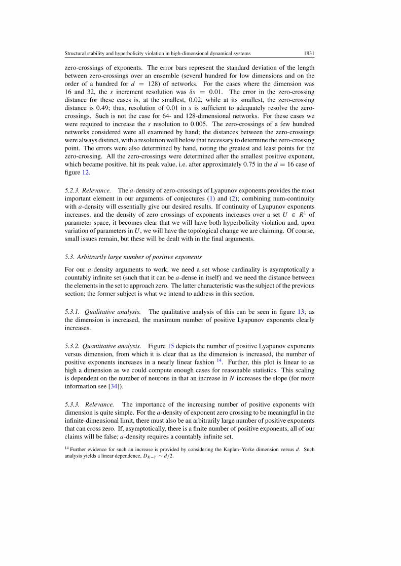
Structural stability and hyperbolicity violation in high-dimensional dynamical systems 1831
zero-crossings of exponents. The error bars represent the standard deviation of the lengthbetween zero-crossings over an ensemble (several hundred for low dimensions and on theorder of a hundred for d = 128) of networks. For the cases where the dimension was16 and 32, the s increment resolution was δs = 0.01. The error in the zero-crossingdistance for these cases is, at the smallest, 0.02, while at its smallest, the zero-crossingdistance is 0.49; thus, resolution of 0.01 in s is sufficient to adequately resolve the zero-crossings. Such is not the case for 64- and 128-dimensional networks. For these cases wewere required to increase the s resolution to 0.005. The zero-crossings of a few hundrednetworks considered were all examined by hand; the distances between the zero-crossingswere always distinct, with a resolution well below that necessary to determine the zero-crossingpoint. The errors were also determined by hand, noting the greatest and least points for thezero-crossing. All the zero-crossings were determined after the smallest positive exponent,which became positive, hit its peak value, i.e. after approximately 0.75 in the d = 16 case offigure 12.
5.2.3. Relevance. The a-density of zero-crossings of Lyapunov exponents provides the mostimportant element in our arguments of conjectures (1) and (2); combining num-continuitywith a-density will essentially give our desired results. If continuity of Lyapunov exponentsincreases, and the density of zero crossings of exponents increases over a set U ∈ R1 ofparameter space, it becomes clear that we will have both hyperbolicity violation and, uponvariation of parameters in U , we will have the topological change we are claiming. Of course,small issues remain, but these will be dealt with in the final arguments.
5.3. Arbitrarily large number of positive exponents
For our a-density arguments to work, we need a set whose cardinality is asymptotically acountably infinite set (such that it can be a-dense in itself) and we need the distance betweenthe elements in the set to approach zero. The latter characteristic was the subject of the previoussection; the former subject is what we intend to address in this section.
5.3.1. Qualitative analysis. The qualitative analysis of this can be seen in figure 13; asthe dimension is increased, the maximum number of positive Lyapunov exponents clearlyincreases.
5.3.2. Quantitative analysis. Figure 15 depicts the number of positive Lyapunov exponentsversus dimension, from which it is clear that as the dimension is increased, the number ofpositive exponents increases in a nearly linear fashion 14. Further, this plot is linear to ashigh a dimension as we could compute enough cases for reasonable statistics. This scalingis dependent on the number of neurons in that an increase in N increases the slope (for moreinformation see [34]).
5.3.3. Relevance. The importance of the increasing number of positive exponents withdimension is quite simple. For the a-density of exponent zero crossing to be meaningful in theinfinite-dimensional limit, there must also be an arbitrarily large number of positive exponentsthat can cross zero. If, asymptotically, there is a finite number of positive exponents, all of ourclaims will be false; a-density requires a countably infinite set.
14 Further evidence for such an increase is provided by considering the Kaplan–Yorke dimension versus d. Suchanalysis yields a linear dependence, DK−Y ∼ d/2.
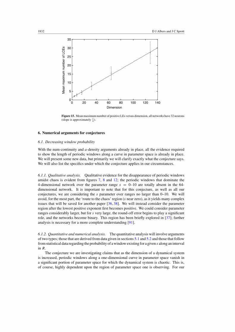
1832 D J Albers and J C Sprott
0
5
10
15
20
25
30
35
0 20 40 60 80 100 120 140
Mea
n m
axim
um n
umbe
r of
LC
Es
Dimension
Figure 15. Mean maximum number of positive LEs versus dimension, all networks have 32 neurons(slope is approximately 1
4 ).
6. Numerical arguments for conjectures
6.1. Decreasing window probability
With the num-continuity and a-density arguments already in place, all the evidence requiredto show the length of periodic windows along a curve in parameter space is already in place.We will present some new data, but primarily we will clarify exactly what the conjecture says.We will also list the specifics under which the conjecture applies in our circumstances.
6.1.1. Qualitative analysis. Qualitative evidence for the disappearance of periodic windowsamidst chaos is evident from figures 7, 8 and 12; the periodic windows that dominate the4-dimensional network over the parameter range s = 0–10 are totally absent in the 64-dimensional network. It is important to note that for this conjecture, as well as all ourconjectures, we are considering the s parameter over ranges no larger than 0–10. We willavoid, for the most part, the ‘route to the chaos’ region (s near zero), as it yields many complexissues that will be saved for another paper [36, 38]. We will instead consider the parameterregion after the lowest positive exponent first becomes positive. We could consider parameterranges considerably larger, but for s very large, the round-off error begins to play a significantrole, and the networks become binary. This region has been briefly explored in [37]; furtheranalysis is necessary for a more complete understanding [91].
6.1.2. Quantitative and numerical analysis. The quantitative analysis will involve argumentsof two types; those that are derived from data given in sections 5.1 and 5.2 and those that followfrom statistical data regarding the probability of a window existing for a given s along an intervalin R.
The conjecture we are investigating claims that as the dimension of a dynamical systemis increased, periodic windows along a one-dimensional curve in parameter space vanish ina significant portion of parameter space for which the dynamical system is chaotic. This is,of course, highly dependent upon the region of parameter space one is observing. For our
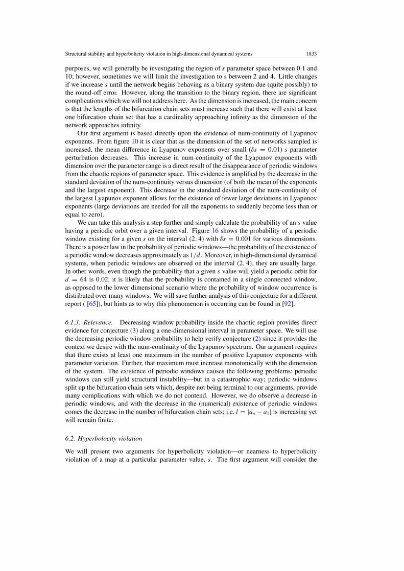
Structural stability and hyperbolicity violation in high-dimensional dynamical systems 1833
purposes, we will generally be investigating the region of s parameter space between 0.1 and10; however, sometimes we will limit the investigation to s between 2 and 4. Little changesif we increase s until the network begins behaving as a binary system due (quite possibly) tothe round-off error. However, along the transition to the binary region, there are significantcomplications which we will not address here. As the dimension is increased, the main concernis that the lengths of the bifurcation chain sets must increase such that there will exist at leastone bifurcation chain set that has a cardinality approaching infinity as the dimension of thenetwork approaches infinity.
Our first argument is based directly upon the evidence of num-continuity of Lyapunovexponents. From figure 10 it is clear that as the dimension of the set of networks sampled isincreased, the mean difference in Lyapunov exponents over small (δs = 0.01) s parameterperturbation decreases. This increase in num-continuity of the Lyapunov exponents withdimension over the parameter range is a direct result of the disappearance of periodic windowsfrom the chaotic regions of parameter space. This evidence is amplified by the decrease in thestandard deviation of the num-continuity versus dimension (of both the mean of the exponentsand the largest exponent). This decrease in the standard deviation of the num-continuity ofthe largest Lyapunov exponent allows for the existence of fewer large deviations in Lyapunovexponents (large deviations are needed for all the exponents to suddenly become less than orequal to zero).
We can take this analysis a step further and simply calculate the probability of an s valuehaving a periodic orbit over a given interval. Figure 16 shows the probability of a periodicwindow existing for a given s on the interval (2, 4) with δs = 0.001 for various dimensions.There is a power law in the probability of periodic windows—the probability of the existence ofa periodic window decreases approximately as 1/d. Moreover, in high-dimensional dynamicalsystems, when periodic windows are observed on the interval (2, 4), they are usually large.In other words, even though the probability that a given s value will yield a periodic orbit ford = 64 is 0.02, it is likely that the probability is contained in a single connected window,as opposed to the lower dimensional scenario where the probability of window occurrence isdistributed over many windows. We will save further analysis of this conjecture for a differentreport ( [65]), but hints as to why this phenomenon is occurring can be found in [92].
6.1.3. Relevance. Decreasing window probability inside the chaotic region provides directevidence for conjecture (3) along a one-dimensional interval in parameter space. We will usethe decreasing periodic window probability to help verify conjecture (2) since it provides thecontext we desire with the num-continuity of the Lyapunov spectrum. Our argument requiresthat there exists at least one maximum in the number of positive Lyapunov exponents withparameter variation. Further, that maximum must increase monotonically with the dimensionof the system. The existence of periodic windows causes the following problems: periodicwindows can still yield structural instability—but in a catastrophic way; periodic windowssplit up the bifurcation chain sets which, despite not being terminal to our arguments, providemany complications with which we do not contend. However, we do observe a decrease inperiodic windows, and with the decrease in the (numerical) existence of periodic windowscomes the decrease in the number of bifurcation chain sets; i.e. l = |an − a1| is increasing yetwill remain finite.
6.2. Hyperbolocity violation
We will present two arguments for hyperbolicity violation—or nearness to hyperbolicityviolation of a map at a particular parameter value, s. The first argument will consider the
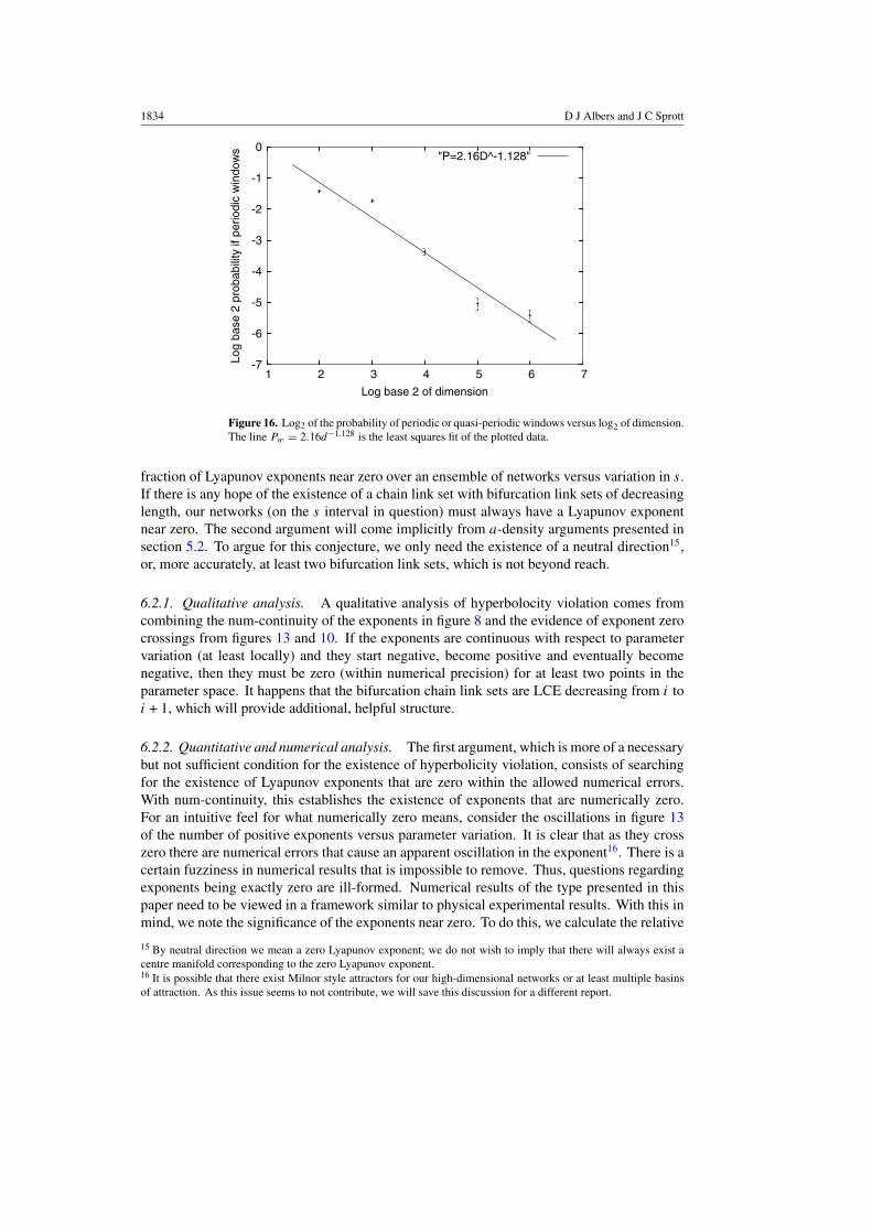
1834 D J Albers and J C Sprott
-7
-6
-5
-4
-3
-2
-1
0
1 2 3 4 5 6 7
Log
base
2 p
roba
bilit
y if
perio
dic
win
dow
s
Log base 2 of dimension
"P=2.16D^-1.128"
Figure 16. Log2 of the probability of periodic or quasi-periodic windows versus log2 of dimension.The line Pw = 2.16d−1.128 is the least squares fit of the plotted data.
fraction of Lyapunov exponents near zero over an ensemble of networks versus variation in s.If there is any hope of the existence of a chain link set with bifurcation link sets of decreasinglength, our networks (on the s interval in question) must always have a Lyapunov exponentnear zero. The second argument will come implicitly from a-density arguments presented insection 5.2. To argue for this conjecture, we only need the existence of a neutral direction15,or, more accurately, at least two bifurcation link sets, which is not beyond reach.
6.2.1. Qualitative analysis. A qualitative analysis of hyperbolocity violation comes fromcombining the num-continuity of the exponents in figure 8 and the evidence of exponent zerocrossings from figures 13 and 10. If the exponents are continuous with respect to parametervariation (at least locally) and they start negative, become positive and eventually becomenegative, then they must be zero (within numerical precision) for at least two points in theparameter space. It happens that the bifurcation chain link sets are LCE decreasing from i toi + 1, which will provide additional, helpful structure.
6.2.2. Quantitative and numerical analysis. The first argument, which is more of a necessarybut not sufficient condition for the existence of hyperbolicity violation, consists of searchingfor the existence of Lyapunov exponents that are zero within the allowed numerical errors.With num-continuity, this establishes the existence of exponents that are numerically zero.For an intuitive feel for what numerically zero means, consider the oscillations in figure 13of the number of positive exponents versus parameter variation. It is clear that as they crosszero there are numerical errors that cause an apparent oscillation in the exponent16. There is acertain fuzziness in numerical results that is impossible to remove. Thus, questions regardingexponents being exactly zero are ill-formed. Numerical results of the type presented in thispaper need to be viewed in a framework similar to physical experimental results. With this inmind, we note the significance of the exponents near zero. To do this, we calculate the relative
15 By neutral direction we mean a zero Lyapunov exponent; we do not wish to imply that there will always exist acentre manifold corresponding to the zero Lyapunov exponent.16 It is possible that there exist Milnor style attractors for our high-dimensional networks or at least multiple basinsof attraction. As this issue seems to not contribute, we will save this discussion for a different report.
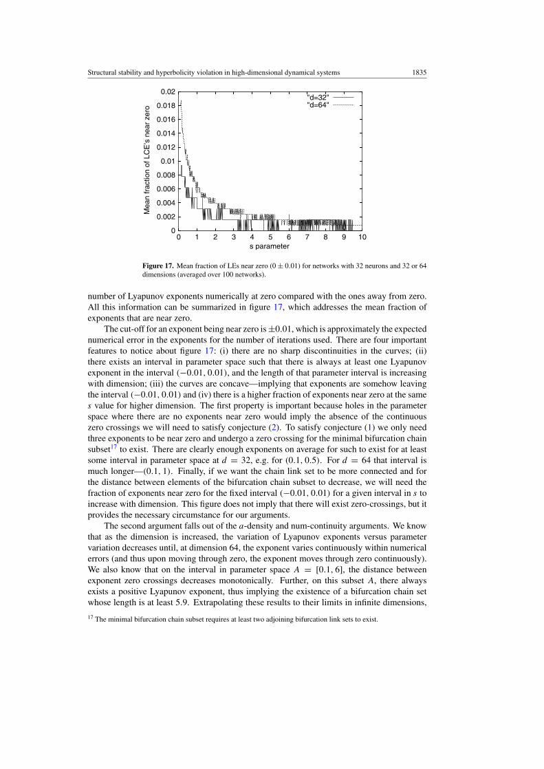
Structural stability and hyperbolicity violation in high-dimensional dynamical systems 1835
0
0.002
0.004
0.006
0.008
0.01
0.012
0.014
0.016
0.018
0.02
0 1 2 3 4 5 6 7 8 9 10
Mea
n fr
actio
n of
LC
E’s
nea
r ze
ro
s parameter
"d=32""d=64"
Figure 17. Mean fraction of LEs near zero (0 ± 0.01) for networks with 32 neurons and 32 or 64dimensions (averaged over 100 networks).
number of Lyapunov exponents numerically at zero compared with the ones away from zero.All this information can be summarized in figure 17, which addresses the mean fraction ofexponents that are near zero.
The cut-off for an exponent being near zero is ±0.01, which is approximately the expectednumerical error in the exponents for the number of iterations used. There are four importantfeatures to notice about figure 17: (i) there are no sharp discontinuities in the curves; (ii)there exists an interval in parameter space such that there is always at least one Lyapunovexponent in the interval (−0.01, 0.01), and the length of that parameter interval is increasingwith dimension; (iii) the curves are concave—implying that exponents are somehow leavingthe interval (−0.01, 0.01) and (iv) there is a higher fraction of exponents near zero at the sames value for higher dimension. The first property is important because holes in the parameterspace where there are no exponents near zero would imply the absence of the continuouszero crossings we will need to satisfy conjecture (2). To satisfy conjecture (1) we only needthree exponents to be near zero and undergo a zero crossing for the minimal bifurcation chainsubset17 to exist. There are clearly enough exponents on average for such to exist for at leastsome interval in parameter space at d = 32, e.g. for (0.1, 0.5). For d = 64 that interval ismuch longer—(0.1, 1). Finally, if we want the chain link set to be more connected and forthe distance between elements of the bifurcation chain subset to decrease, we will need thefraction of exponents near zero for the fixed interval (−0.01, 0.01) for a given interval in s toincrease with dimension. This figure does not imply that there will exist zero-crossings, but itprovides the necessary circumstance for our arguments.
The second argument falls out of the a-density and num-continuity arguments. We knowthat as the dimension is increased, the variation of Lyapunov exponents versus parametervariation decreases until, at dimension 64, the exponent varies continuously within numericalerrors (and thus upon moving through zero, the exponent moves through zero continuously).We also know that on the interval in parameter space A = [0.1, 6], the distance betweenexponent zero crossings decreases monotonically. Further, on this subset A, there alwaysexists a positive Lyapunov exponent, thus implying the existence of a bifurcation chain setwhose length is at least 5.9. Extrapolating these results to their limits in infinite dimensions,
17 The minimal bifurcation chain subset requires at least two adjoining bifurcation link sets to exist.
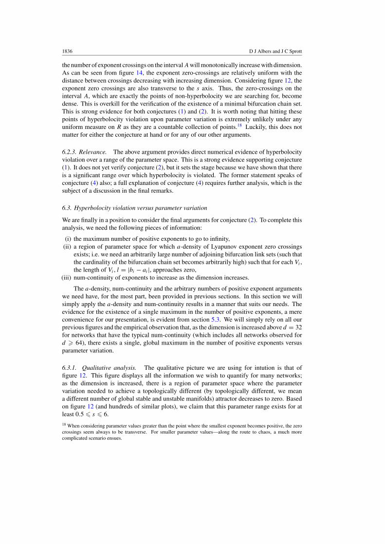
1836 D J Albers and J C Sprott
the number of exponent crossings on the interval A will monotonically increase with dimension.As can be seen from figure 14, the exponent zero-crossings are relatively uniform with thedistance between crossings decreasing with increasing dimension. Considering figure 12, theexponent zero crossings are also transverse to the s axis. Thus, the zero-crossings on theinterval A, which are exactly the points of non-hyperbolocity we are searching for, becomedense. This is overkill for the verification of the existence of a minimal bifurcation chain set.This is strong evidence for both conjectures (1) and (2). It is worth noting that hitting thesepoints of hyperbolocity violation upon parameter variation is extremely unlikely under anyuniform measure on R as they are a countable collection of points.18 Luckily, this does notmatter for either the conjecture at hand or for any of our other arguments.
6.2.3. Relevance. The above argument provides direct numerical evidence of hyperbolocityviolation over a range of the parameter space. This is a strong evidence supporting conjecture(1). It does not yet verify conjecture (2), but it sets the stage because we have shown that thereis a significant range over which hyperbolocity is violated. The former statement speaks ofconjecture (4) also; a full explanation of conjecture (4) requires further analysis, which is thesubject of a discussion in the final remarks.
6.3. Hyperbolocity violation versus parameter variation
We are finally in a position to consider the final arguments for conjecture (2). To complete thisanalysis, we need the following pieces of information:
(i) the maximum number of positive exponents to go to infinity,(ii) a region of parameter space for which a-density of Lyapunov exponent zero crossings
exists; i.e. we need an arbitrarily large number of adjoining bifurcation link sets (such thatthe cardinality of the bifurcation chain set becomes arbitrarily high) such that for each Vi ,the length of Vi , l = |bi − ai |, approaches zero,
(iii) num-continuity of exponents to increase as the dimension increases.
The a-density, num-continuity and the arbitrary numbers of positive exponent argumentswe need have, for the most part, been provided in previous sections. In this section we willsimply apply the a-density and num-continuity results in a manner that suits our needs. Theevidence for the existence of a single maximum in the number of positive exponents, a mereconvenience for our presentation, is evident from section 5.3. We will simply rely on all ourprevious figures and the empirical observation that, as the dimension is increased above d = 32for networks that have the typical num-continuity (which includes all networks observed ford � 64), there exists a single, global maximum in the number of positive exponents versusparameter variation.
6.3.1. Qualitative analysis. The qualitative picture we are using for intution is that offigure 12. This figure displays all the information we wish to quantify for many networks;as the dimension is increased, there is a region of parameter space where the parametervariation needed to achieve a topologically different (by topologically different, we meana different number of global stable and unstable manifolds) attractor decreases to zero. Basedon figure 12 (and hundreds of similar plots), we claim that this parameter range exists for atleast 0.5 � s � 6.
18 When considering parameter values greater than the point where the smallest exponent becomes positive, the zerocrossings seem always to be transverse. For smaller parameter values—along the route to chaos, a much morecomplicated scenario ensues.
Structural stability and hyperbolicity violation in high-dimensional dynamical systems 1837
6.3.2. Quantitative and numerical analysis. Let us now complete our arguments forconjecture (2). For this we need a subset of the parameter space, B ⊂ R1, such that somevariation of s ∈ B will lead to a topological change in the map f in the form of a change in thenumber of global stable and unstable manifolds. Specifically, we need B = ⋃
Vi = V , whereVi and Vi+1 share a limit point and are disjoint. Further, we need the variation in s neededfor the topological change to decrease monotonically with dimension on V . More precisely,on the bifurcation chain set, U , the distance between elements must decrease monotonicallywith increasing dimension. We will argue in three steps: first, we will argue that, for each f
with a sufficiently large number of dimensions, there will exist an arbitrarily large number ofexponent zero crossings (equivalent to an arbitrarily large number of positive exponents); nextwe will argue that the zero crossings are relatively smooth and finally, we will argue that thezero crossings form an a-dense set on V —or on the bifurcation chain set, l = |bi − ai | → 0as d → ∞. This provides strong evidence supporting conjecture (2).
Assuming a sufficiently large number of dimensions, verification of conjecture (1) givesthe existence of the bifurcation chain set and the existence of the adjoining bifurcation link sets.The existence of an arbitary number of positive Lyapunov exponents and thus an arbitrarilylarge number of zero-crossings follows from section 5.3. That the bifurcation chain set hasan arbitrarily large number of elements, #U → ∞ is established by conjecture (3) because,without periodic windows, every bifurcation link set will share a limit point with anotherbifurcation link set. From section 5.1, the num-continuity of the exponents persists for asufficiently large number of dimensions; thus, the Lyapunov exponents will cross throughzero. Finally, section 5.2 tells us that the Lyapunov exponent zero-crossings are a-dense; thus,for all ci ∈ U , |ci − ci+1| → 0, where ci and ci+1 are sequential elements of U . For our work,we can identify U as U ⊂ [0.5, 6]. We could easily extend the upper bound to much greaterthan 6 for large dimensions (d � 128). How high the upper bound can be extended will bediscussed in further work. It is useful to note that the bifurcation link sets are LCE decreasingwith increasing s. This is not necessary to our arguments, but it is a nice added structure thataids our intuition. The LCE decreasing property exists due to the existence of the single, globalmaximum in the maximum number of positive Lyapunov exponents followed by an apparentexponential decrease in the number of positive Lyapunov exponents.
6.3.3. Relevance. The above arguments provide direct evidence of conjectures (2) and (4)for a one-dimensional curve (specifically an interval) in parameter space for our networks.This evidence also suggests the persistence of chaos in high-dimensional networks withperturbations on higher-dimensional surfaces in parameter space. Finally, despite theseemingly inevitable topological change upon minor parameter variation, the topologicalchange is quite benign.
7. Fitting everything together
Having finished with our specific analysis, we now put our work in the context of other work,both of a more mathematical and a more practical and experimental nature. In this spirit, wewill provide a brief summary of our arguments followed by a discussion of how our resultsmesh with various theoretical results from dynamical systems and turbulence.
7.1. Summary of arguments
7.1.1. Periodic window probability decreasing: conjecture 3. The conjecture that the prob-ability of periodic windows for a given s value along an interval in parameter space decreases
1838 D J Albers and J C Sprott
with increasing dimension upon the smallest positive Lyapunov exponent becoming positiveis initially clear from considering the Lyapunov spectra of neural networks versus parametervariation for networks of increasing size (figures 7 and 8). We show that as the dimension isincreased, the observed probability of periodic windows decreases inversely with increasingdimension. This analysis is independent of the num-continuity analysis, and the results fromthe analysis of num-continuity and periodic window probability decrease reinforce each other.The mechanism that this conjecture provides is the lengthening of the bifurcation chain set.
Further investigations of this phenomenon will follow in a later report. For other relatedresults see [35, 65, 92–94].
7.1.2. Hyperbolicity violation: conjecture 1. The intuition for this conjecture arises fromobserving that for high-dimensional systems, there exists at least one Lyapunov exponent thatstarts negative, becomes positive, then becomes negative again; thus, if it behaves numericallycontinuously, it must pass through zero for some parameter value s.
To verify this conjecture, we presented two different arguments. The first argument was anecessary but not sufficient condition for hyperbolicity violation. We show that over a sizeableinterval in parameter space there exists a Lyapunov exponent very near zero, and the fractionof the total number of Lyapunov exponents that are near zero increases over a larger intervalof parameter space as the dimension is increased. The second argument was based on thea-density of exponent zero crossings, the num-continuity of the exponents as the dimensionincreased and the increasing number of positive exponents with dimension. Both argumentstogether help imply an interval of parameter space such that on that interval the number ofparameter values such that hyperbolicity is violated is increasing.
It is important to note that it is possible that hyperbolicity can be violated along the orbit.If hyperbolicity is violated along the orbit for a measurable set of values, but the mean of eachof the exponents averaged along the orbit is non-zero, then the diagnostics in this paper willbe inconclusive. Insight into hyperbolicity violation along a given orbit can be obtained byconsidering a histogram of the exponents and observing whether the tails of the distributionsof the exponents near zero overlap zero. Such an analysis is done on a case by case basis.Because this paper represents a statistical study, we have reserved such an analysis for anotherpaper.
7.1.3. Existence of codimension-ε bifurcation set: conjecture 2. The intuition for thisargument follows from observing that the peak in the number of positive Lyapunov exponentstends toward a spike of increasing height and decreasing width as the dimension is increased.This, with some sort of continuity of exponents, argues for a decrease in distance betweenexponent zero crossings.
Summarizing the arguments regarding conjecture (2), with increasing dimension we haveincreased num-continuity of Lyapunov exponents; increasing number of positive Lyapunovexponents and a-density of Lyapunov exponent zero crossings (thus all the exponents arenot clustered on top of each other). Thus, on a finite set in parameter space, there is anarbitrary number of exponents that move smoothly from negative values to positive valuesand back to negative values. Further, these exponents are relatively evenly spaced. Thus, theset in parameter space for which hyperbolicity is violated is increasingly dense; and with anarbitrary number of violations available, the perturbation of the parameter required to force atopological change (a change in the number of positive exponents) becomes small.
Further evidence of continuous topological change is provided by the smooth variation ofthe plot of the Kaplan–Yorke dimension versus s that corresponds to figure 13 [35].
Structural stability and hyperbolicity violation in high-dimensional dynamical systems 1839
7.1.4. Non-genericity of structural stability: conjecture 4. As previously mentioned, it couldappear that our results contradict Robbin [3], Robinson [4] and Mane [5]. We will discussspecifically how our results fit with theirs in section 7.3.1. In the current discussion, weinterpret our results in a numerical context.
We claim to have found a subset of parameter space that, in the limit of infinite dimensions,has dense hyperbolicity violation. This could be interpreted to imply that we have located aset for which strict hyperbolicity does not imply structural stability because the C1 changes inthe parameter give rise to topologically different behaviour. The key issue is that in numericalsimulations, there do not exist infinitesimals or infinite-dimensional limits19. Rather, we canspeak as to how behaviour arises and how limits behave along the path to the ideal. Wehave found a subset of parameter space that can approximate (with unlimited computing)arbitrarily closely a set for which hyperbolicity will not imply structural stability. Thus, anexperimentalist or a numerical scientist might see behaviour that apparently violates the resultsof Robbin [3], Robinson [4] and Mane [5]; yet it will not be strictly violating those theorems.The key point of this conjecture is that we can observe apparent violation of the structuralstability conjecture, but the violation (on a Lebesgue measure zero set) occurs as smooth, notcatastrophic, topological change. (In section 7.3.1 we will further discuss our results as theyrelate to those of Robbin [3], Robinson [4] and Mane [5].)
7.2. Fitting our results in with the space of Cr functions: how our network selection methodaffects our view of function space
The act of performing a numerical experiment induces a measure on whatever is beingexperimented upon. A measure, in a very general sense, provides a method of determiningthe volume that a set occupies in its ambient space (for a formal treatment, see [95]). Usuallythat method provides a specific mechanism of measuring lengths of a covering interval. Then,the entire space is covered with the aforementioned intervals, and their collective volume issummed. One of the key issues is how the intervals are weighted. For instance, consideringthe real line with the standard Gaussian measure imposed upon it; the interval [−1, 1] containsthe majority of the volume of the entire interval [−∞, ∞]. Our method of weighting networksselects fully connected networks with random Gaussian weights. Thus, in the limit of highdimension and large number of neurons, very weakly connected networks will be rare becausethe Gaussian statistics of the weights will be dominant. Likewise, fully connected networkswhere all the weights have the same strength (up to an order of magnitude) will also beuncommon. One can argue whether or not the measure we utilize realistically representsthe function space of nature, but those arguments are fundamentally ill-formed because theycannot be answered without either specific information about the natural system with whichour framework is being compared or the existence of some type of invariant measure. Thebest hope for specifying connections between natural systems, other computational modelsand a neural network construction such as the point presented here is using the aforementionednotion of prevalence. Nevertheless, the product measure we impose does cover the entire spaceof neural networks noted in section 1, although all sets do not have equal likelihood of beingselected, and thus our results must be interpreted with this in mind.
A second key issue regards how the ambient space is split into intervals or, in a numericalsense, how the grain of the space is constructed. We will again introduce a simpler case forpurposes of illustration, followed by a justification of why the simpler case and our networkframework are essentially equivalent. Begin with Rn and select each coordinate (vi) in the
19 Note that in previous sections we do use words like, ‘in the infinite-dimensional limit’. It is for reasons such asthese (and many others) that we are only putting forth conjectures and not theorems; this distinction is not trivial.
1840 D J Albers and J C Sprott
vector v = {v1, v2, · · · , vn} ∈ Rn from a normal, i.i.d. distribution with mean zero, varianceone. Next, suppose that we are attempting to see every number and every number combination.This will be partially achieved by the random number selection process mentioned above,and it is further explored by sweeping the variance, i.e. selecting a scalar s ∈ R, 0 � s
and sweeping s over the positive real line, sv. This establishes two meshes, one for theindividual vectors, which is controlled by how finely the s parameter is varied, and anothermesh that controls how the initial coordinates are selected. These two combined meshesdetermine the set of combinations of coordinates that will be observed. If one considershow this affects vector selection in, say, R3, for simplicity, both in the initial vector selectionand in the vector sweeping, it is clear how R3 will be carved out. The point is that we candirectly associate how we carve up our neural network function space with how we carve upthe neural network weight space. To understand how our neural network selection processworks, simply associate v with the vectors in the ω matrix and s with the scaling parameters. This keeps the view of our function space largely in standard Euclidean space. Of coursethere is the last remaining issue of the amplitude terms, the β. Apply the same type ofanalysis to the β as for the ω. Of course, initially it would seem that the scaling parameteris missing, but note that multiplying the β by s, in our networks, is essentially equivalentto multiplying the ω by s. To understand this, consider the one-dimensional network, withone neuron:
xt = β0 + β1 tanh(sω0 + sω1(β0 + β1 tanh(sω0 + sω1xt−1))). (38)
It is clear from this that inserting s inside tanh will sweep the β, but inserting s outside thesquashing function will miss sweeping the ω0 bias term.20 What this all amounts to is aheuristic construction of a probe space (relative to the measures on the parameter space) forembeddings of Cr dynamical systems using neural networks. More formal constructions aretopics of current work.
Summarizing, it should be clear that the measures we utilize will capture the entire spaceof neural networks we are employing. Yet, it should also be clear that we will not select eachnetwork with equal probability. Moreover, the measure we impose is a product measure,not a joint probability measure where there is a co-dependence between the parameters.This hopefully has a significant impact on our conclusions and results—for there is toomuch diversity in natural systems to be caught by a single measure on a space of universalapproximators. A complete connection between network structure and dynamics, in anunderstandable language, is yet out of reach (as opposed to, say, for spherical harmonics),but this is a current direction of research. Various research programs for quantifyingvarious spaces of neural networks and their dynamics by the measures on the weights arecurrently underway using tools such as information geometry [53, 96]. Nevertheless, weclaim that our framework gives a complete picture of the space of Cr maps of compactsets to compact sets with the Sobolev metric from the perspective of a particular productmeasure.
7.3. Our results related to other results in dynamical systems
As promised throughout, we will now connect our results with various theorems and conjecturesin the field of dynamical systems. This will hopefully help put our work in context and increaseits understandability.
20 Recalling section 2.1.4, we actually do a little more with the β than we mention here; the previous argument is simplymeant to give a (mathematically imprecise) picture of how our experiment carves out the space of neural networks.
Structural stability and hyperbolicity violation in high-dimensional dynamical systems 1841
7.3.1. Structural stability theory and conjecture 4. It is now time to address the apparentconflict between our observations and the structural stability theorems of Robbin [3], Robinson[4] and Mane [5]. We would like to begin by noting that we do not doubt the validity orcorrectness of any of these results. In fact, any attempt to use our techniques and resultsto provide a counter example to the theorems of Robbin, Robinson or Mane involves amisunderstanding of what our methods do and imply.
In conjecture (4) we claim, in an intuitive sense, that along a one-dimensional curve inparameter space, our dynamical systems are hyperbolic with Lebesgue measure one. Yet, wecan still find subsets that are measure zero, yet a-dense, for which our dynamical systems arepartially hyperbolic rather than hyperbolic. The motivation for the above statement roughlyderives from thinking of a turbulent fluid. In this circumstance, the number of unstablemanifolds can be countably infinite, and upon varying, say, the viscosity, from very low to veryhigh, one would have a countable number of exponents becoming positive over a finite lengthof parameter space. Yet, all the limits of this sort and all the intuition about what will happenin the infinite-dimensional limit are just ideas. There are limits to what we can compute; theredo not exist infinite-dimensional limits or infinitesimals in numerical computing, and asidefrom the existence of convergence theorems, we are unable to draw conclusions beyond whatthe data say. Thus, our results do not provide a counter-example to the stability conjecture.Rather, a key point of our results is that we do observe, in a realistic numerical setting, structuralinstability upon small parameter variation. It is useful to think instead of structural stability asan open condition on our parameter space whose endpoints correspond to the points of structuralinstability—the points of bifurcations in turbulence. These disjoint open sets are precisely thebifurcation link subsets, Vi , for which the map f is structurally stable. As the dimensionis increased, the lengths of the Vi decrease dramatically and may fall below numericalor experimental resolution. Thus, the numerical or experimental scientist might observetopological variation in the form of a variation in the number of positive Lyapunov exponentsupon parameter variation in systems that should be (and technically are) structurally stableaccording to the work of Robbin, Robinson and Mane; i.e. the scientist might observe structuralinstability. This is the very practical difference between numerical computing and the world ofstrict mathematics. (Recall we were going to connect structural stability theory closer to reality;the former statement is as far as we will go in this paper.) The good news is that even thoughobserved structural stability might be lost, it is lost in a very meek manner—the topologicalchanges are very slight, just as seems to be observed in many turbulent experimental systems.Further, partial hyperbolicity is not lost, and the dynamically stable characteristics of stableergodicity seem to be preserved; although, we obviously cannot make a strict mathematicalstatement.
Thus, rather than claiming our results are contrary to those of Robbin [3], Robinson [4], andMane [5], our results speak to both what might be seen of those theorems in high-dimensionaldynamical systems and how their results are approached upon increasing the dimension of adynamical system.
It is worth noting that, given a typical 64-dimensional network, if we fixed s at such apoint that there was an exponent zero crossing, we believe (based on preliminary results) thatthere will exist many perturbations of other parameters that leave the exponent zero crossingunaffected. However, these perturbations are apparently of very small Lebesgue measure andof a small codimension set in parameter space, i.e. we believe we can find, in the constructionwe use, perturbations that will leave the seemingly transversal intersection of an exponentwith 0 at a particular s value unchanged; yet, these parameter changes must be small. A veryinteresting question is whether the same could be said if the measure on the weight space wasa joint rather than a product measure.
1842 D J Albers and J C Sprott
7.3.2. Stable ergodicity. In this study we are particularly concerned with the interplay,along a parametrized curve, of how often partial hyperbolicity is encountered versus stricthyperbolicity. It should be noted that if a dynamical system is hyperbolic, it is partiallyhyperbolic. All the neural networks we considered were at least partially hyperbolic; we foundno exceptions. Many of the important questions regarding partially hyperbolic dynamicalsystems lie in showing the conditions under which such systems are stably ergodic. We willnow discuss this in relation to our results and methods.
Pugh and Shub [60] put forth the following conjecture regarding partial hyperbolicity andstable ergodicity.
Conjecture 5 (Pugh and Shub [60] conjecture 3). Let f ∈ Diff2µ(M) where M is compact.
If f is partially hyperbolic and essentially accessible then f is ergodic.
The strongest result that has been shown to date regarding their conjecture is in [97].
Theorem 3 (Stable ergodicity theorem (theorem 0.1 [97])). Let f be C2, volume preserv-ing, partially hyperbolic and centre bunched. If f is essentially accessible then f is ergodicand, in fact, has the Kolmogorov property.
A diffeomorphism is partially hyperbolic if it satisfies the conditions of definition (7).Ergodic behaviour implies that, upon breaking the attractor into measurable sets, Ai , for f
applied to each measurable set for enough time, f n(Ai) will intersect every other measurable setAj . This implies a weak sense of recurrence; for instance, quasi-periodic orbits, chaotic orbits,and some random processes are at least colloquially ergodic. More formally, a dynamicalsystem is ergodic if and only if almost every point of each set visits every set with positivemeasure. The accessibility property simply formalizes a notion of one point being able to reachanother point. Given a partially hyperbolic dynamical system, f : X → X such that there isa splitting on the tangent bundle T M = Eu ⊕ Ec ⊕ Es , and x, y ∈ X, y is accessible fromx if there is a C1 path from x to y whose tangent vector lies in Eu ∩ Es and vanishes finitelymany times (these paths are denoted u-s-paths). The diffeomorphism f is centre bunchedif the spectra of Tf (as defined in section 2.2) corresponding to the stable (T sf ), unstable(T uf ) and (T cf ) central directions lie in thin, well separated annuli (see [97] for the mostrecent and general formulation; the radii of the annuli are technical and are determined bythe Holder continuity of the diffeomorphism). Lastly, let us note that a dynamical system iscalled stably ergodic if, given f ∈ Diff2
µ(M) (again M compact), there is a neighbourhood,f ∈ Y ⊂ Diff2
µ(M), such that every g ∈ Y is ergodic with respect to µ.The current proofs of the Pugh–Shub stable ergodicity theorem require the dynamical
system to be Lebesgue measure preserving—or non-dissipative. The primary technique of theproofs is to very carefully select a positive measure set and then very carefully move it alongthe u-s-paths in such a way that all the positive measure sets are visited while the original setretains positive measure. Doing this hinges on absolute continuity with respect to Lebesguemeasure on the orbit with respect to both the stable and unstable manifolds. Needless to say,it is difficult to prove that a dissipative dynamical system is ergodic. But, while the argumentshinge on absolute continuity on both the stable and unstable manifolds, it is believed that theresults do not. The results from this paper reinforce this viewpoint. One tactic of weakening thearea-preserving condition is to consider partially hyperbolic dynamical systems with negative(or positive) central exponents along the orbit (e.g. modified Pesin theory). In this vein, usingtheorems 10 and 11 and corollary 12 of [79], it can be concluded that partially hyperbolicdynamical systems with negative central exponents and with a particular SRB-like measure(see [79] for details) will be ergodic.
Numerical verification of ergodicity can be somewhat difficult because the modeller wouldhave to watch each point and verify that eventually the trajectory returns very close to every
Structural stability and hyperbolicity violation in high-dimensional dynamical systems 1843
other point on the orbit (i.e. it satisfies the Birkoff hypothesis). Doing this for a few points is, ofcourse, possible; but doing it for a high-dimensional attractor for any sizable number of pointscan be extremely time consuming. For d high enough, we observe a single SRB measure. Thiscan be seen in figure 8 where every s value has a different initial condition. If this is a robustresult, and using results from Burns et al [79], if the central exponents can be shown to be neg-ative, ergodicity will follow. Because we have not studied the exponents along the orbit in thiswork, we cannot use this argument to claim that ergodicity is existent and stable in the ensembleof systems we studied. Checking the accessibility criterion seems to pose similar problems; infact, it is hoped that accessibility is the sufficient recurrence condition for ergodic behaviour.Thus, it should be no surprise that accessibility would be difficult to check numerically (it hasbeen shown to be C1 dense [98]). However, in essence, ergodicity is a notion capturing indivis-ibility of the attractor relative to a measure. The key point is that all positive measure sets arevisited by all orbits with probability one. The most obvious, and it is thought, the primary meansof splitting up an attractor is the existence of neutral directions or zero Lyapunov exponents(see the ‘stacked Anosov’ in [7] for a simple example). Considering figures 8, 9 and 12, andthe overall argument presented, it is clear that the persistence of zero exponents with respect toparameter change in the systems we study is unlikely. Moreover, figures 4–6 demonstrate thatquantities dependent upon the SRB measures for calculation converge in the uniform mannerexpected of an ergodic system. Of course, showing that one has explored all the variationsinside the neighbourhood (f ∈)Y ⊂ Diff2
µ(M) is impossible; thus, claiming that we have, ina mathematically rigorous way, observed stable ergodicity as the predominant characteristicwould be premature. However, generalizing our results using notions of prevalence is a topic ofcurrent work and does not seem out of reach. What we can say is that we have never observed adynamical system, within our construction, that is not on a compact set and is not partially hy-perbolic; moreover, systems seemed to become more stably ergodic as the dimension increased.Thus, our results provide evidence that the conjecture of Pugh and Shub, which does not requirearea preservation or absolute continuity with respect to the stable and unstable manifolds, is ontrack. For more information with respect to the mathematics discussed above, see [7, 19, 59].
Comparing conjecture (5) with theorem (3), the required extra hypothesis for the proofof the theorem is only centre bunching of the spectrum of Tf . It is likely that the centrebunching hypothesis has been weakened as far is it can be for the current arguments. As itstands, the spectra that we observe, which are strongly reminiscent of what might be expectedin turbulent-like dynamics, do appear to satisfy the current centre bunching criterion.21 Wecannot comment on its necessity. Moreover, considering similar numerical work done byothers, and vaguely combining the circular law ([22–24]) with matrix product results ( [99]),it is likely that the centre bunching criterion as it stands is not crucial for dissipative systems.
7.3.3. Palis’s conjectures. Palis [9] stated many stability conjectures based upon the lastthirty years of developments in dynamical systems that we wish to relate to the results in thepresent paper [9].
Conjecture 6 (Global conjecture on the finitude of attractors and their metricstability [9]).
(I) Denseness of finitude of attractors—there is a Cr (r � 1) dense set D of dynamics suchthat any element of D has finitely many attractors whose union of basins of attraction hastotal probability;
21 It is worth noting that in section 31 of Landau and Lifshitz’s fluid mechanics book [100], they give physical reasonswhy one might expect a centre bunching type of spectrum or at least a finite number of exponents near zero, in turbulentfluids.
1844 D J Albers and J C Sprott
(II) Existence of physical (SRB) measures—the attractors of the elements in D support aphysical measure;
(III) Metric stability of basins of attraction—for any element in D and any of its attractors, foralmost all small Cr perturbations in generic k-parameter families of dynamics, k ∈ N ,there are finitely many attractors whose union of basins is nearly (Lebesgue) equal to thebasin of the initial attractor; such perturbed attractors support a physical measure;
(IV) Stochastic stability of attractors—the attractors of elements of D are stochastically stablein their basins of attraction;
(V) For generic families of one-dimensional dynamics, with total probability in parameterspace, the attractors are either periodic sinks or carry an absolutely continuous invariantmeasure.
In the portion of parameter space we examine, multiple attractors are exceedingly rare,thus yielding support for (I). This can be seen in figures 8, 9 and 12 where the initial conditionswere not held fixed, yet the exponents varied continuously—leading to the conclusion thatfor such systems there is only one attractor. However, if the dynamics we observe are indeedturbulent-like, this is not surprising since turbulent systems rarely, if ever, exhibit multiple SRBmeasures. Item (II) is supported by figures 4–6 that show convergence of measure-dependentquantities. Claim (III) is particularly intriguing given the construction we utilize because of thepotential of using neural networks as a probe space for the embeddings defined in section 2.1.5,thus utilizing the notions of prevalence to quantify (III) in a computational setting.
The next conjecture of Palis is directly related to the problems addressed in this work.
Conjecture 7 (Palis [9] conjecture II). In any dimension, the diffeomorphisms exhibitingeither a homoclinic tangency or a (finite) cycle of hyperbolic periodic orbits with differentstable dimensions (heterodimensiopnal cycle) are Cr dense in the complement of the closureof the hyperbolic ones.
Let us decompress this and then discuss how our results fit with it. Begin by defining the space ofd-dimensional Cr diffeomorphisms as X. Next, break that space up as follows: A = {x ∈ X|xexhibits a homoclinic tangency or a finite cycle of hyperbolic periodic orbits with differentstable dimensions } and B = {x ∈ X|x is hyperbolic }. Thus B is the set of hyperbolic,aperiodic diffeomorphisms, and A is the set of periodic orbits or partially hyperbolic orbits.The conjecture states that A is dense in the complement of the closure of B; thus, A can be densein B. With respect to our results, the partially hyperbolic diffeomorphisms (diffeomorphismswith homoclinic tangencies) can be dense within the set of hyperbolic diffeomorphisms. Ourconjectures claim to find a subset of our one-dimensional parameter space such that partiallyhyperbolic diffeomorphisms will, in the limit of high dimensions, be dense. In other words,our work not only agrees with Palis’s conjecture II (and subsequently his conjecture III), butour work provides evidence confirming Palis’s conjectures. Of course, we do not claim toprovide mathematical proofs but rather strong numerical evidence supporting Palis’s ideas.
7.4. Final remarks
Finally, let us briefly summarize:
Statement of results 2 (Summary). Assuming our particular conditions and our particularspace of Cr dynamical systems as per section 1, there exists a collection of bifurcation linksubsets (V ) such that, in the limit of countably infinite dimensions, we have numerical evidence
Structural stability and hyperbolicity violation in high-dimensional dynamical systems 1845
for the following.
Conjecture 1: on the above-mentioned setV , strict hyperbolicity will be violated a-densely.Conjecture 2: on the above-mentioned set V , the number of stable and/or unstable
manifolds will change under parameter variation below numerical precision.Conjecture 3: on the above-mentioned set V , the probability of the existence of a periodic
window for a gives s on a specific parameter interval decreases inversely with dimension.Conjecture 4: on the above-mentioned set V , hyperbolic dynamical systems are not
structurally stable within numerical precision with measure one with respect to Lebesguemeasure in parameter space.
In a measure-theoretic sense, hyperbolic systems occupy all the space, but the partiallyhyperbolic dynamical systems (with non-empty centre manifolds) can be a-dense on V .Intuitively, if there are countable dimensions—thus countable Lyapunov exponents, then oneof two things can happen upon parameter variation:
(i) there would have to be a persistent homoclinic tangency—or some other sort of non-transversal intersection between stable and unstable manifolds that is persistent toparameter changes;
(ii) there can be, at most, countably many parameter points such that there are non-transversalintersections between stable and unstable manifolds.
We claim to observe (ii). We also see that for our networks, each exponent in the spectrumconverges to a unique (within numerical resolution) value over a variety of initial conditions.This confirms both the usefulness and validity of our techniques and provides strong evidencefor the prevalence of ergodic-like behaviour. Further, upon parameter variation, the ergodicbehaviour is seemingly preserved; thus, we also have strong evidence of a prevalence of stableergodic behaviour under parameter variation.
Acknowledgments
The authors would like to thank J R Albers, D Feldman, C McTague, J Supanich and JThompson for a careful and thoughtful reading of this manuscript. Comments provided byK Burns were indispensable and aided in the correctness and readability of this manuscript.DJA would like to thank R A Bayliss, K Burns, W D Dechert, D Feldman, C McTague, JRobbin, C R Shalizi and J Supanich for many helpful discussions and advice. DJA wouldlike to give special thanks to J P Crutchfield for much guidance, many fruitful discussionsand support throughout this project—his support and insight contributed significantly to thispaper. The computing for the project was done on the Beowulf cluster at the Santa Fe Instituteand was partially supported at the Santa Fe Institute under the Networks, Dynamics Programfunded by the Intel Corporation under the Computation, Dynamics, and Inference Program viaSFI’s core grant from the National Science and MacArthur Foundations. Direct support forDJA was provided by NSF grants DMR-9820816 and PHY-9910217 and DARPA AgreementF30602-00-2-0583.
References
[1] Chern S and Smale S (ed) 1970 Global Analysis (Proc. Symp. Pure Math. vol 14) (Berkeley, CA: AMS)[2] Palis J and Smale S 1970 Structural stability theorems Global Analysis (Proc. Symp. Pure Math. vol 14)
ed S Chern and S Smale (Berkeley, CA: AMS)[3] Robbin J 1971 Ann. Math. 94 447[4] Robinson C 1971/1973 Dynamical Systems (Salvador: Academic) pp 443–9
1846 D J Albers and J C Sprott
[5] Mane R 1988 Publ. Math. IHES 66 161[6] Poincare H 1929 Sur les proprietes des fonctions definies par les euations aux differences partieles., Oeuvres
(Paris: Gauthier-Villars)[7] Burns K, Pugh C, Shub M and Wilkinson A 2001 Smooth Ergodic Theory and its Applications (Proc. Symp.
Pure Math. vol 69) (Berkeley, CA: American Mathematical Society) pp 327–66[8] Pugh C and Shub M 2003 Bull. Am. Math. Soc. 41 1[9] Palis J 2000 Asterisque 261 339
[10] Nitecki Z 1971 Differentiable Dynamics: An Introduction to the Orbit Structure of Diffeomorphisms (Boston,MA: MIT Press)
[11] Bonatti C, Diaz L and Viana M 2004 Dynamics Beyond Uniform Hyperbolicity: A Global Geometric andProbabilistic Perspective (Berlin: Springer)
[12] Palis J and Smale S 1970 Global Analysis (Proc. Symp. Pure Math. vol 14) (Berkeley, CA: AMS)[13] Smale S 1967 Bull. Am. Math. Soc. 73 747[14] Newhouse S 1979 Publ. Math. IHES 50 101[15] Lorenz E N 1963 J. Atmosph. Sci. 20 130[16] Milnor J 1985 Commun. Math. Phys.[17] Sommerer J and Ott E 1993 Nature 365 135[18] Kaneko K 2002 Phys. Rev. E 66 055201[19] Pugh C and Shub M 1997 J. Complexity 13 125[20] Brin M I and Pesin J B 1974 Math. USSR Izv. 8 177 (English Transl.)[21] Sompolinsky H, Crisanti A and Sommers H J 1988 Phys. Rev. Lett.[22] Girko V 1994 Random Oper. Stoch. Eqns 2 235[23] Edelman A 1997 J. Multivariate Anal. 60 203[24] Bai Z D 1997 Ann. Probab. 25 494[25] Doyon B, Cessac B, Quoy M and Samuelides M 1993 Int. J. Bifurc. Chaos 3 279[26] Doyon B, Cessac B, Quoy M and Samuelides M 1994 Acta Biotheo. 42 215[27] Cessac B, Doyon B, Quoy M and Samuelides M 1994 Physica D 74 24[28] Cessac B 1995 J. Phys. I (France) 5 409[29] Moynot O and Samuelides M 2002 Probab. Theory Relat. Fields 123 41[30] Hornik K, Stinchocombe M and White H 1990 Neural Netw. 3 551[31] Sauer T, Yorke J and Casdagli M 1991 J. Stat. Phys. 65 579[32] Grassberger P 1989 Phys. Scr. 40 346[33] Kaneko K 1986 Collapse of Tori and Genesis of Chaos in Dissipative Systems (Singapore: World Scientific)[34] Albers D J, Sprott J C and Crutchfield J P 2006 High-dimensional dynamics, scaling laws and general dynamics,
in preparation[35] Albers D J 2004 PhD Thesis University of Wisconsin in Madison[36] Albers D J and Sprott J C 2006 Probability of a local bifurcation type from a fixed point: a random matrix
perspective J. Stat. Phys. submitted (Preprint nlin.CD/0510060)[37] Albers D J, Sprott J C and Dechert W D 1998 Int. J. Bifurc. Chaos 8 1463[38] Albers D J and Sprott J C 2006 Physica D submitted[39] Takens F 1981 Dynamical Systems and Turbulence (Warwick) (Lecture Notes in Mathematics vol 898) ed D Rand
and L Young (Berlin: Springer) pp 366–81[40] Noakes L 1991 Int. J. Bifurc. Chaos 4 867[41] Gencay R and Dechert W D 1992 Physica D 59 142[42] Ott W and Yorke J 2003 SIAM J. Appl. Dyn. Syst. 3 297[43] Ott W and Yorke J A 2005 Bull. Am. Math. Soc. 42 263[44] Hunt B R, Sauer T and Yorke J A 1992 Bull. Am. Math. Soc. 27 217[45] Hunt B R, Sauer T and Yorke J A 1993 Bull. Am. Math. Soc. 28 2306[46] Albers D J, Crutchfield J P and J C Sprott 2006 Geometric variation in high-dimensional high entropy dynamical
systems, in preparation[47] Hornik K, Stinchocombe M and White H 1989 Neural Netw. 2 359[48] Adams R and Fournier J J F 2003 Sobolev Spaces 2nd edn (Amsterdam: Elsevier)[49] Hebey E 1999 Nonlinear Analysis on Manifolds: Sobolev Spaces and Inequalities (Berkeley, CA: American
Mathematical Society)[50] P L’Ecuyer 1988 Commun. ACM 31 742[51] Press W A and Teukolsky S A 1992 Comput. Phys. 6 522[52] Albers D J, Sprott J C and W D Dechert Intelligent Engineering Systems Through Artifical Neural Networks
vol 6 (ASME) pp 17–22
Structural stability and hyperbolicity violation in high-dimensional dynamical systems 1847
[53] Amari S 2000 Differential and Algebraic Geometry of Multilayer Perceptrons vol 3 (IEICE Trans. Fundamentals)[54] Sprott J C 2003 Chaos and Time-series Analysis (Oxford: Oxford University Press)[55] Kantz H and Schreiber T 2003 Nonlinear Time Series Analysis 2nd edn (Cambridge: Cambridge University
Press)[56] Smale S 1966 Am. J. Math. 88 491[57] Anosov D V 1967 Proc. Steklov Inst. Math. 90 1[58] Hirsch M W Pugh C C and Shub M 1977 Invariant Manifolds (Springer Lecture Notes in Mathematics) vol 583
(Berlin: Springer)[59] Burns K, Dolgopyat D and Pesin Y 2002 J. Stat. Phys. 108 927[60] Pugh C and Shub M 2000 J. Eur. Math. Soc. 2 1[61] Barreira L and Pesin Y 2002 Lyapunov Exponents and Smooth Ergodic Theory (Berkeley, CA: AMS)[62] Katok A and Hasselblatt B 1995 Introduction to the Modern Theory of Dynamical Systems (Encyclopedia of
Mathematics and its Applications) vol 54 (Cambridge: Cambridge University Press)[63] Mane R 1987 Ergodic Theory and Differentiable Dynamics (Berlin: Springer)[64] Young L-S 2002 J. Stat. Phys. 108 733[65] Albers D J, Sprott J C and Crutchfield J P 2006 Persistant chaos in high dimensions Phys. Rev. E at press
(Preprint nlin.CD/0504040)[66] Ruelle D 1979 Publ. Math. I.H.E.S. 50 27[67] Oseledec V I 1968 Tras. Moscow Math. Soc. 19 197[68] Katok A 1980 Publ. Math. I.H.E.S. 51 137[69] Ruelle D 1982 Ann. Math. 115 243[70] Pesin Y B 1976 Soviet Math. Dokl. 17 196 (English Transl.)[71] Pesin Y B 1976 Math. USSR Izv. 10 1261 (English Transl.)[72] Pesin Y B 1977 Russ. Math. Surv. 32 55 (English Transl.)[73] Robinson C 1976 J. Diff. Eqns 22 28[74] Brin M and Stuck G 2004 Introduction to Dynamical Systems (Cambridge: Cambridge University Press)[75] Loeve 1977 Probability Theory I (Berlin: Springer)[76] Ledrappier F and Young L-S 1985 Ann. Math. 122 509[77] Ledrappier F and Strelcyn J M 1982 Ergod. Theory Dynam. Sys. 2 203[78] Ruelle D 1976 Am. J. Math 98 619[79] Burns K, Dolgopyat D, Pesin Y and Pollicott M Preprint[80] Benedicks M and Carleson L 1991 Ann. Math 133 73[81] Benedicks M and L-S Young 1993 Invent. Math 112 541[82] Sotomayor J 1973 Dynamical Systems pp 549–60[83] Wiggins S 1988 Global Bifurcations and Chaos: Analytical Methods (AMS) (Berlin: Springer)[84] Benettin G, Galgani L, Giorgilli A and J-M Strelcyn 1979 Meccanica 15 9[85] Benettin G, Galgani L, Giorgilli A and J-M Strelcyn 1979 Meccanica 15 21[86] Shimada I and Nagashima T 1979 Prog. Theor. Phys. 61 1605[87] Geist K, Parlitz U and Lauterborn W 1990 Prog. Theor. Phys. 83 875[88] Dechert W D and Gencay R 1996 Physica D 90 40[89] McDonald E J and Higham D J 2001 Electron. Trans. Numer. Anal. 12 234[90] Dieci L and Vleck E V 1995 Appl. Numer. Math. 17 275[91] Albers D J and Sprott J C contact [email protected] for notes[92] Barreto E, Hunt B, Grebogi C and Yorke J A 1997 Phys. Rev. Lett. 78 4561[93] Banerjee S, Yorke J A and Grebogi C 1998 Phys. Rev. Lett. 80 3049[94] Potapov A and Ali M K 2000 Phys. Lett. A 277 310[95] Wheeden R L and Zygmund A 1977 Measure and Integral Monographs and Textbooks in Pure and Applied
Mathematics vol 43 (New York: Dekker)[96] Amari S, Nagaoka H and S-I Amari 2001 Methods of Information Geometry (Translations of Mathematical
Monographs) (AMS)[97] Burns K and Wilkinson A Preprint math.DS/0510234[98] Wilkinson A and Dolgopyat D 2003 Asterisque 287 33–60[99] 1986 Random Matrices and Their Applications (Contemoporary Mathematics) vol 50 (AMS)[100] Landau D and Lifshitz L 1989 Fluid Mechanics (Oxford: Pergamon)