1/18

Hyperbolicity of the heat equation

TFMST 2019

3rd IFAC Workshop on Thermodynamic Foundation of Mathematical Systems Theory

Guilherme Ozorio Cassol, Stevan Dubljevic

Department of Chemical and Materials Engineering

July 4, 2019

2/18

Outline

1 Background & Motivation

2 The heat equation

3 The Stefan Problem

4 Conclusions

Background

&

Motivation

The heat

equation

The Stefan

Problem

Conclusions

References

3/18

Background & Motivation

Diffusive transport are generally described by Fourier’s law:

Parabolic nature: Any initial disturbance in the material

body is propagated instantly1

Hyperbolicity: physically relevant and desired property →physically meaningful finite speed of phenomena propagation

To eliminate this unphysical feature: modified Fourier law to

take into account the thermal inertia → finite speed of

propagation2

1Christo I. Christov and P. M. Jordan. “Heat conduction paradox involving second-sound propagation in moving media.”. In: Physical

review letters 94 15 (2005), pp. 154–301.

2C. Cattaneo. “On a form of heat equation which eliminates the paradox of instantaneous propagation”. In: C. R. Acad. Sci. Paris

(1958), pp. 431–433, P. Vernotte. “Les paradoxes de la theorie continue de l’equation de la chaleur”. In: C. R. Acad. Sci. Paris 246

(1958), pp. 3154–3155, D. Jou, J. Casas-Vazquez, and G. Lebon. Extended irreversible thermodynamics (3rd Edition). Springer, 2001.

Background

&

Motivation

The heat

equation

The Stefan

Problem

Conclusions

References

4/18

Background & Motivation

Application to a Stefan Problem is considered:

Specific type of boundary value problem (moving boundary

position needs to be determined);

Generally focusing in the heat distribution, in a phase

changing medium;Examples:

Diffusion of heat in the melting/solidification of ice;

Fluid flow in porous media;

Shock waves in gas dynamics3.

3L.I. Rubenstein. The Stefan problem, by L.I. Rubenstein. Translations of mathematical monographs. American Mathematical

Society, 1971.

Background

&

Motivation

The heat

equation

The Stefan

Problem

Conclusions

References

5/18

The Heat Conduction Paradox

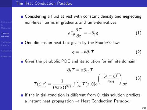
Considering a fluid at rest with constant density and neglecting

non-linear terms in gradients and time-derivatives:

ρCp∂T

∂t= −∂ζq (1)

One dimension heat flux given by the Fourier’s law:

q = −k∂ζT (2)

Gives the parabolic PDE and its solution for infinite domain:

∂tT = α∂ζζT

T (ζ, t) =1

(4παt)3/2

∫∞−∞ T (z , 0)e

−(z − ζ)2

4αt

dz

(3)

If the initial condition is different from 0, this solution predicts

a instant heat propagation → Heat Conduction Paradox.

Background

&

Motivation

The heat

equation

The Stefan

Problem

Conclusions

References

6/18

The modified Fourier’s Law

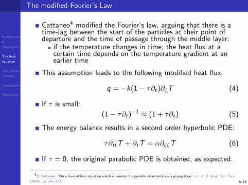
Cattaneo4 modified the Fourier’s law, arguing that there is atime-lag between the start of the particles at their point ofdeparture and the time of passage through the middle layer:

if the temperature changes in time, the heat flux at acertain time depends on the temperature gradient at anearlier time

This assumption leads to the following modified heat flux:

q = −k(1− τ∂t)∂ζT (4)

If τ is small:

(1− τ∂t)−1 ≈ (1 + τ∂t) (5)

The energy balance results in a second order hyperbolic PDE:

τ∂ttT + ∂tT = α∂ζζT (6)

If τ = 0, the original parabolic PDE is obtained, as expected.

4C. Cattaneo. “On a form of heat equation which eliminates the paradox of instantaneous propagation”. In: C. R. Acad. Sci. Paris

(1958), pp. 431–433.

Background

&

Motivation

The heat

equation

The Stefan

Problem

Conclusions

References

7/18

Comparison in a one dimension heat diffusion problem

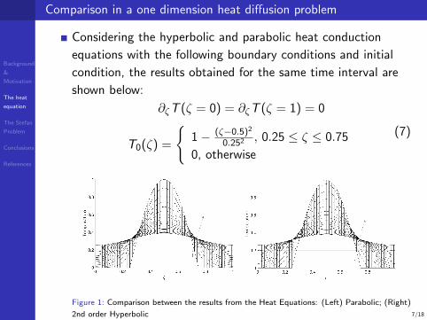
Considering the hyperbolic and parabolic heat conduction

equations with the following boundary conditions and initial

condition, the results obtained for the same time interval are

shown below:

∂ζT (ζ = 0) = ∂ζT (ζ = 1) = 0

T0(ζ) =

{1− (ζ−0.5)2

0.252 , 0.25 ≤ ζ ≤ 0.75

0, otherwise

(7)

Figure 1: Comparison between the results from the Heat Equations: (Left) Parabolic; (Right)

2nd order Hyperbolic

Background

&

Motivation

The heat

equation

The Stefan

Problem

Conclusions

References

8/18

Comparison in a one dimension heat diffusion problem

0 0.1 0.2 0.3 0.4 0.5

Time

0

0.05

0.1

0.15

0.2

0.25

Tem

pera

ture

= 0.05, =0.01

= 0.05, =0.02

= 0.075, =0.02

= 0.075, =0.01

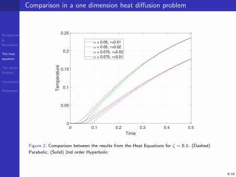
Figure 2: Comparison between the results from the Heat Equations for ζ = 0.1: (Dashed)

Parabolic; (Solid) 2nd order Hyperbolic

Background

&

Motivation

The heat

equation

The Stefan

Problem

Conclusions

References

9/18

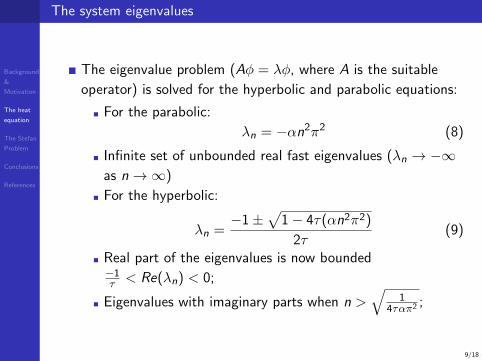
The system eigenvalues

The eigenvalue problem (Aφ = λφ, where A is the suitable

operator) is solved for the hyperbolic and parabolic equations:

For the parabolic:

λn = −αn2π2 (8)

Infinite set of unbounded real fast eigenvalues (λn → −∞as n→∞)

For the hyperbolic:

λn =−1±

√1− 4τ(αn2π2)

2τ(9)

Real part of the eigenvalues is now bounded−1τ < Re(λn) < 0;

Eigenvalues with imaginary parts when n >√

14ταπ2 ;

Background

&

Motivation

The heat

equation

The Stefan

Problem

Conclusions

References

10/18

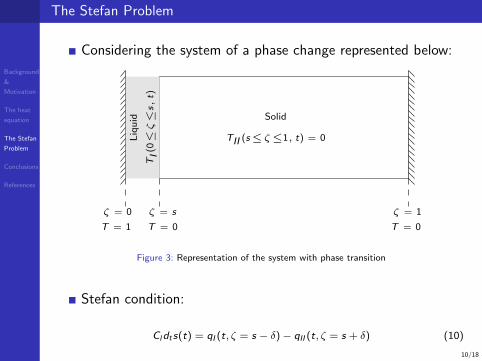
The Stefan Problem

Considering the system of a phase change represented below:

ζ = 0

T = 1

ζ = s

T = 0

ζ = 1

T = 0

Liq

uid

TI

(0≤ζ≤

s,t)

Solid

TII (s≤ζ≤1, t) = 0

Figure 3: Representation of the system with phase transition

Stefan condition:

Cldts(t) = qI (t, ζ = s − δ)− qII (t, ζ = s + δ) (10)

Background

&

Motivation

The heat

equation

The Stefan

Problem

Conclusions

References

11/18

The Stefan Problem

The following assumptions are considered:

Transition temperature: TC = 0;

Initial condition: T0(ζ) = 0;

Temperature at ζ = 1 is the transition temperature

(T (ζ = 1) = TC );No heat sinks or sources;

Simplify the model to a one phase problem (only the liquid

phase has a temperature profile that needs to be found) and

only this phase has a heat flux:

Cldts(t) = qI (t, ζ = s − δ); (11)

Background

&

Motivation

The heat

equation

The Stefan

Problem

Conclusions

References

12/18

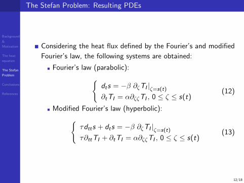
The Stefan Problem: Resulting PDEs

Considering the heat flux defined by the Fourier’s and modified

Fourier’s law, the following systems are obtained:

Fourier’s law (parabolic):{dts = −β ∂ζTI |ζ=s(t)

∂tTI = α∂ζζTI , 0 ≤ ζ ≤ s(t)(12)

Modified Fourier’s law (hyperbolic):{τdtts + dts = −β ∂ζTI |ζ=s(t)

τ∂ttTI + ∂tTI = α∂ζζTI , 0 ≤ ζ ≤ s(t)(13)

Background

&

Motivation

The heat

equation

The Stefan

Problem

Conclusions

References

13/18

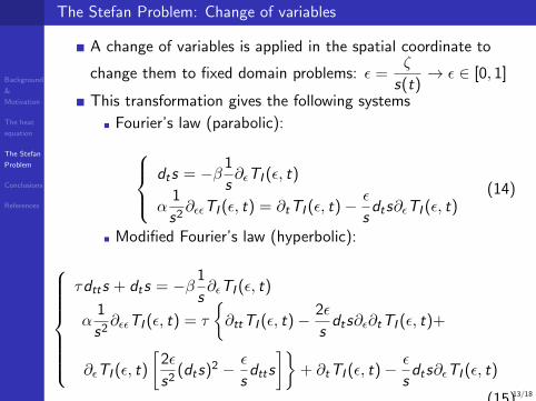
The Stefan Problem: Change of variables

A change of variables is applied in the spatial coordinate to

change them to fixed domain problems: ε =ζ

s(t)→ ε ∈ [0, 1]

This transformation gives the following systems

Fourier’s law (parabolic):dts = −β 1

s∂εTI (ε, t)

α1

s2∂εεTI (ε, t) = ∂tTI (ε, t)− ε

sdts∂εTI (ε, t)

(14)

Modified Fourier’s law (hyperbolic):

τdtts + dts = −β 1

s∂εTI (ε, t)

α1

s2∂εεTI (ε, t) = τ

{∂ttTI (ε, t)− 2ε

sdts∂ε∂tTI (ε, t)+

∂εTI (ε, t)

[2ε

s2(dts)2 − ε

sdtts

]}+ ∂tTI (ε, t)− ε

sdts∂εTI (ε, t)

(15)

Background

&

Motivation

The heat

equation

The Stefan

Problem

Conclusions

References

14/18

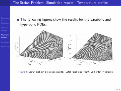
The Stefan Problem: Simulation results - Temperature profiles

The following figures show the results for the parabolic and

hyperbolic PDEs:

Figure 4: Stefan problem simulation results: (Left) Parabolic; (Right) 2nd order Hyperbolic

Background

&

Motivation

The heat

equation

The Stefan

Problem

Conclusions

References

15/18

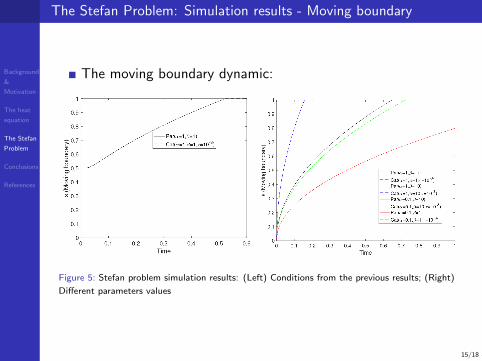
The Stefan Problem: Simulation results - Moving boundary

The moving boundary dynamic:

Figure 5: Stefan problem simulation results: (Left) Conditions from the previous results; (Right)

Different parameters values

Background

&

Motivation

The heat

equation

The Stefan

Problem

Conclusions

References

16/18

Conclusions

The analysis of the behavior of the heat diffusion considering hyper-

bolic and parabolic equations was accomplished. It was possible to see

the difference between these two equations, which shows the finite speed

of propagation of the hyperbolic equation.

A Stefan problem was also considered and the results show that the inter-

face dynamic for the hyperbolic equation is similar to the parabolic for the

conditions considered, but the former equation’s finite speed of propa-

gation would be more desirable to represent the dynamics of the actual

physical system.

Future work will analyze the difference between these two equations

when control problems are considered.

Background

&

Motivation

The heat

equation

The Stefan

Problem

Conclusions

References

17/18

Thank You

Background

&

Motivation

The heat

equation

The Stefan

Problem

Conclusions

References

18/18

References I

C. Cattaneo. “On a form of heat equation which eliminates the paradox of

instantaneous propagation”. In: C. R. Acad. Sci. Paris (1958), pp. 431–433.

Christo I. Christov and P. M. Jordan. “Heat conduction paradox involving

second-sound propagation in moving media.”. In: Physical review letters 94 15

(2005), pp. 154–301.

D. Jou, J. Casas-Vazquez, and G. Lebon. Extended irreversible thermodynamics

(3rd Edition). Springer, 2001.

L.I. Rubenstein. The Stefan problem, by L.I. Rubenstein. Translations of

mathematical monographs. American Mathematical Society, 1971.

P. Vernotte. “Les paradoxes de la theorie continue de l’equation de la chaleur”.

In: C. R. Acad. Sci. Paris 246 (1958), pp. 3154–3155.