overview hyperbolicity stability
TRANSCRIPT
OverviewHyperbolicity
Stability
I: Hyperbolicity, stability and geometry
Robin Pemantle
Current Developments in Mathematics, 18 November 2011
Pemantle Hyperbolicity, stability and applications

OverviewHyperbolicity
Stability
DefinitionsExamplesPhilosophy and organization
Two related concepts
These lectures are about two related properties of polynomials,hyperbolicity and stability.
These notions have been at the heart of some fundamental resultsin very different fields, dating from 60 years ago to the present.
I will survey the development and key uses of these concepts,devoting the first lecture largely to hyperbolicity and the second tostability.
Pemantle Hyperbolicity, stability and applications

OverviewHyperbolicity
Stability
DefinitionsExamplesPhilosophy and organization
Definitions
A homogeneous polynomial p of degree m is said to be hyperbolicin direction x ∈ Rd if p(y + ix) 6= 0 for all y ∈ Rd.
A polynomial q is said to be stable if q(z) 6= 0 whenever eachcoordinate zj is in the strict upper half plane.
Proposition 1 (hyperbolicity vs. stability)
A real homogeneous polynomial is stable if and only if it ishyperbolic in every direction in the positive orthant. �
Notation: d will denote the number of variables and m the degree.
Pemantle Hyperbolicity, stability and applications

OverviewHyperbolicity
Stability
DefinitionsExamplesPhilosophy and organization
What you are missing, part I:
Definition of hyperbolicity in the inhomogeneous case
Note: once we have restricted to the homogenous case, we mayalso assume without loss of generality that p is real: forhomogeneous polynomials, hyperbolicity implies that some multipleis real.
Pemantle Hyperbolicity, stability and applications

OverviewHyperbolicity
Stability
DefinitionsExamplesPhilosophy and organization
Real roots
Proposition 2 (location of zeros)
q(y + ix) 6= 0 for all y if and only if q(x) 6= 0 and z 7→ q(y + zx)has all real zeros when y is real.
Proof: Absorb the real part of zx into y. �
Pemantle Hyperbolicity, stability and applications

OverviewHyperbolicity
Stability
DefinitionsExamplesPhilosophy and organization
Example: Lorentzian quadratic
Let p be the Lorentzian quadratic t2 − x22 − · · · − x2
d, where wehave renamed x1 as “t” because of its interpretation as the timeaxis in spacetime; then p is hyperbolic in every timelike direction,that is, for each direction x with p(x) > 0.
The time axis is left-right
Pemantle Hyperbolicity, stability and applications

OverviewHyperbolicity
Stability
DefinitionsExamplesPhilosophy and organization
Example: coordinate planes
The coordinate function xj is hyperolic in direction y if and only ifyj 6= 0 (this is true for any linear polynomial).
It is obvious from the definition that the product of polynomialshyperbolic in direction y is again hyperbolic in direction y.
It follows that∏d
j=1 xj is hyperbolic in every direction notcontained in a coordinate plane, that is, in every open orthant.
Pemantle Hyperbolicity, stability and applications

OverviewHyperbolicity
Stability
DefinitionsExamplesPhilosophy and organization
More examples
Early works developing the theory of hyperbolic functions seem totreat the Lorentzian quadratic as the only motivating example,though they discuss a few others to show that the theory is moregeneral. The generality turned out to be useful in contexts thatwere only dreamed of much later. Along with these contexts camenew examples.
We won’t have time here to discuss two sources of examples,namely lacunas and self-concordant barrier functions. We will,however, discuss the example of rational Taylor series. It turns outthat any polynomial, when localized at a point on the boundary ofits amoeba, is hyperbolic. More on these notions later, but here isa picture.
Pemantle Hyperbolicity, stability and applications
OverviewHyperbolicity
Stability
DefinitionsExamplesPhilosophy and organization
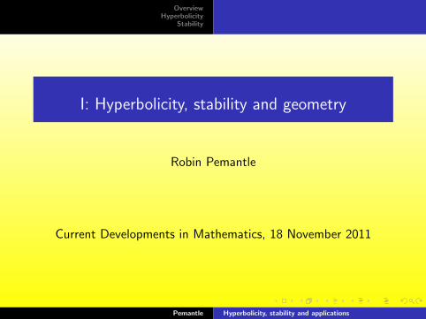
Example: Fortress polynomial
w4 − u2w2 − v2w2 +9
25u2v2
is the projective localization of the denominator (cleaned up a bit)of the so-called Fortress generating polynomial. It followsfrom [BP11, Proposition 2.12] that this polynomial is hyperbolic.
Pemantle Hyperbolicity, stability and applications

OverviewHyperbolicity
Stability
DefinitionsExamplesPhilosophy and organization
Another example from combinatorics
This is from a 1-parameter family of hyperbolic polynomials. It isirreducible (the collar in the middle is not a flat plane) except forone parameter value.
Pemantle Hyperbolicity, stability and applications

OverviewHyperbolicity
Stability
DefinitionsExamplesPhilosophy and organization
Ubiquity of zeros of polynomials
“The one contribution of mine that I hope will beremembered has consisted in pointing out that all sortsof problems of combinatorics can be viewed as problemsof the location of the zeros of certain polynomials...”
– Gian-Carlo Rota (1985)cited by Borcea, Branden and Liggett (2009)
Also: PDE’s/harmonic analysis, probability, number theory, ...
Pemantle Hyperbolicity, stability and applications

OverviewHyperbolicity
Stability
DefinitionsExamplesPhilosophy and organization
Organization
The first lecture will be more geometric. The important propertiesof hyperbolic functions are related to convexity and to cones ofhyperbolicity. Applications are to propagation of wave-like PDE’s,inverse Fourier transforms, and their application to analyticcombinatorics.
The second lecture has a more algebraic flavor. Closure propertiesof the class of stable polynomials play a large role. Many of theapplications concern determinants.
Pemantle Hyperbolicity, stability and applications
OverviewHyperbolicity
Stability
Evolution of wavelike PDE’sRiesz kernel, and propagation in a coneMorse deformations and application to Taylor coefficients
Hyperbolicity
Pemantle Hyperbolicity, stability and applications

OverviewHyperbolicity
Stability
Evolution of wavelike PDE’sRiesz kernel, and propagation in a coneMorse deformations and application to Taylor coefficients
Major uses of hyperbolicity
Highlights:
* Garding’s necessary and sufficient condition for stability of theevolution of a wave-like PDE (1951). See also Petrovsky (1947).
* Atiyah-Bott-Garding’s computation of inverse Fourier transformsand lacunas for homogeneous rational functions (1970).
* Interior methods for convex programming (1997).
* Asymptotics of Taylor coefficients for rational functions (2011).
Pemantle Hyperbolicity, stability and applications

OverviewHyperbolicity
Stability
Evolution of wavelike PDE’sRiesz kernel, and propagation in a coneMorse deformations and application to Taylor coefficients
Major uses of hyperbolicity
Highlights:
* Garding’s necessary and sufficient condition for stability of theevolution of a wave-like PDE (1951).
See also Petrovsky (1947).
* Atiyah-Bott-Garding’s computation of inverse Fourier transformsand lacunas for homogeneous rational functions (1970).
* Interior methods for convex programming (1997).
* Asymptotics of Taylor coefficients for rational functions (2011).
Pemantle Hyperbolicity, stability and applications

OverviewHyperbolicity
Stability
Evolution of wavelike PDE’sRiesz kernel, and propagation in a coneMorse deformations and application to Taylor coefficients
Major uses of hyperbolicity
Highlights:
* Garding’s necessary and sufficient condition for stability of theevolution of a wave-like PDE (1951). See also Petrovsky (1947).
* Atiyah-Bott-Garding’s computation of inverse Fourier transformsand lacunas for homogeneous rational functions (1970).
* Interior methods for convex programming (1997).
* Asymptotics of Taylor coefficients for rational functions (2011).
Pemantle Hyperbolicity, stability and applications

OverviewHyperbolicity
Stability
Evolution of wavelike PDE’sRiesz kernel, and propagation in a coneMorse deformations and application to Taylor coefficients
Major uses of hyperbolicity
Highlights:
* Garding’s necessary and sufficient condition for stability of theevolution of a wave-like PDE (1951). See also Petrovsky (1947).
* Atiyah-Bott-Garding’s computation of inverse Fourier transformsand lacunas for homogeneous rational functions (1970).
* Interior methods for convex programming (1997).
* Asymptotics of Taylor coefficients for rational functions (2011).
Pemantle Hyperbolicity, stability and applications

OverviewHyperbolicity
Stability
Evolution of wavelike PDE’sRiesz kernel, and propagation in a coneMorse deformations and application to Taylor coefficients
Properties
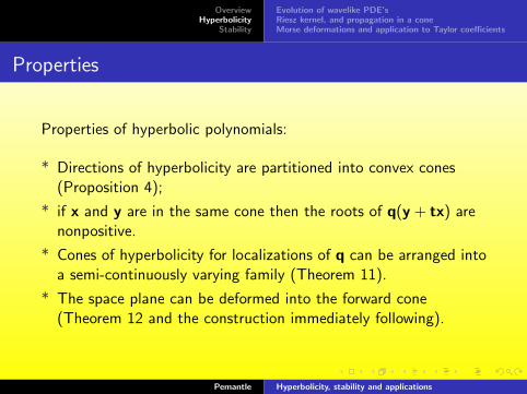
Properties of hyperbolic polynomials:
* Directions of hyperbolicity are partitioned into convex cones(Proposition 4);
* if x and y are in the same cone then the roots of q(y + tx) arenonpositive.
* Cones of hyperbolicity for localizations of q can be arranged intoa semi-continuously varying family (Theorem 11).
* The space plane can be deformed into the forward cone(Theorem 12 and the construction immediately following).
Pemantle Hyperbolicity, stability and applications

OverviewHyperbolicity
Stability
Evolution of wavelike PDE’sRiesz kernel, and propagation in a coneMorse deformations and application to Taylor coefficients
Properties
Properties of hyperbolic polynomials:
* Directions of hyperbolicity are partitioned into convex cones(Proposition 4);
* if x and y are in the same cone then the roots of q(y + tx) arenonpositive.
* Cones of hyperbolicity for localizations of q can be arranged intoa semi-continuously varying family (Theorem 11).
* The space plane can be deformed into the forward cone(Theorem 12 and the construction immediately following).
Pemantle Hyperbolicity, stability and applications

OverviewHyperbolicity
Stability
Evolution of wavelike PDE’sRiesz kernel, and propagation in a coneMorse deformations and application to Taylor coefficients
What you are missing, part II:
Properties of hyperbolicity in the inhomogeneous case
Pemantle Hyperbolicity, stability and applications

OverviewHyperbolicity
Stability
Evolution of wavelike PDE’sRiesz kernel, and propagation in a coneMorse deformations and application to Taylor coefficients
Stable evolution of PDE’s
Let q be a polynomial in d variables and denote by Dq theoperator q(∂/∂x) obtained by replacing each xi by ∂/∂xi.
Let r be a vector in Rd, let Hr be the hyperplane orthogonal to r,and consider the equation
Dq(f) = 0 (1)
in the halfspace {r · x ≥ 0} with boundary conditions specified onHr (typically, f and its first d− 1 normal derivatives).
We say that (1) evolves stably in direction r if convergence of theboundary conditions to 0 implies convergence of the solution to 0.Convergence here means uniform convergence of the function andits derivatives on compact sets.
Pemantle Hyperbolicity, stability and applications

OverviewHyperbolicity
Stability
Evolution of wavelike PDE’sRiesz kernel, and propagation in a coneMorse deformations and application to Taylor coefficients
Stable evolution of PDE’s
Let q be a polynomial in d variables and denote by Dq theoperator q(∂/∂x) obtained by replacing each xi by ∂/∂xi.
Let r be a vector in Rd, let Hr be the hyperplane orthogonal to r,and consider the equation
Dq(f) = 0 (1)
in the halfspace {r · x ≥ 0} with boundary conditions specified onHr (typically, f and its first d− 1 normal derivatives).
We say that (1) evolves stably in direction r if convergence of theboundary conditions to 0 implies convergence of the solution to 0.
Convergence here means uniform convergence of the function andits derivatives on compact sets.
Pemantle Hyperbolicity, stability and applications

OverviewHyperbolicity
Stability
Evolution of wavelike PDE’sRiesz kernel, and propagation in a coneMorse deformations and application to Taylor coefficients
Stable evolution of PDE’s
Let q be a polynomial in d variables and denote by Dq theoperator q(∂/∂x) obtained by replacing each xi by ∂/∂xi.
Let r be a vector in Rd, let Hr be the hyperplane orthogonal to r,and consider the equation
Dq(f) = 0 (1)
in the halfspace {r · x ≥ 0} with boundary conditions specified onHr (typically, f and its first d− 1 normal derivatives).
We say that (1) evolves stably in direction r if convergence of theboundary conditions to 0 implies convergence of the solution to 0.Convergence here means uniform convergence of the function andits derivatives on compact sets.
Pemantle Hyperbolicity, stability and applications

OverviewHyperbolicity
Stability
Evolution of wavelike PDE’sRiesz kernel, and propagation in a coneMorse deformations and application to Taylor coefficients
r
Pemantle Hyperbolicity, stability and applications

OverviewHyperbolicity
Stability
Evolution of wavelike PDE’sRiesz kernel, and propagation in a coneMorse deformations and application to Taylor coefficients
Garding’s Theorem
Theorem 3 ([Gar51, Theorem III])
The equation Dqf = 0 evolves stably in direction r if and only if qis hyperbolic in direction r.
Let us see why this should be true.
We begin with the observation that if ξ ∈ Cd is any vector withq(ξ) = 0 then fξ(x) := exp(iξ · x) is a solution to Dqf = 0. (Oursolutions are allowed to be complex but live on Rd.)
Pemantle Hyperbolicity, stability and applications

OverviewHyperbolicity
Stability
Evolution of wavelike PDE’sRiesz kernel, and propagation in a coneMorse deformations and application to Taylor coefficients
Forward direction
Stability implies hyperbolicity:
Assume WLOG that r = (0, . . . , 0, 1).
Suppose q is not hyperbolic. Then at least one line parallel to r hasa pair of complex roots, meaning that there is a ξ with q(ξ) = 0and ξ = (a1, . . . , ad−1, ad ± bi), with {ai} and b real and b 6= 0.
Picking b < 0, the function fξ grows exponentially in direction r.For large λ, the function fλξ grows even faster.
Sending λ→∞, we may take initial conditions going to zero suchthat fλξ(r) = 1 for all λ.
Pemantle Hyperbolicity, stability and applications

OverviewHyperbolicity
Stability
Evolution of wavelike PDE’sRiesz kernel, and propagation in a coneMorse deformations and application to Taylor coefficients
Argument for the reverse direction
The other direction is harder, but here is a hand-waving argument.
Hyperbolicity imples stability:
Suppose q is hyperbolic. For every real r′ = (r1, . . . , rd−1) infrequency space there are d real values of rd such thatq(r) := q(r′, rd) = 0. For each such r, the function fr is a solutionto Dq(f) = 0 traveling unitarily.
These d solutions are a unitary basis for the space Vr′ that theyspan, of solutions to (1) that restrict on Hξ to eir′·x, and the sameis true at any later time.
Pemantle Hyperbolicity, stability and applications

OverviewHyperbolicity
Stability
Evolution of wavelike PDE’sRiesz kernel, and propagation in a coneMorse deformations and application to Taylor coefficients
Heuristic
Handwave: Because the vector space has dimension d over anyspatial frequency, we can believe we have all the solutions. Theyall evolve unitarily. Thus, writing any boundary conditionsf = g0, f ′ = g1, . . . , f(d−1) = gd−1 as an integral of functions fr,unitary evolution implies a Parseval-type relation, meaning thatsmall boundary conditions will lead to small values at any positivetime.
Pemantle Hyperbolicity, stability and applications

OverviewHyperbolicity
Stability
Evolution of wavelike PDE’sRiesz kernel, and propagation in a coneMorse deformations and application to Taylor coefficients
Discussion
I That hyperbolicity is the “right” condition for stability ofPDE’s is not in question: Garding’s criterion is necessary andsufficient.
I Hyperbolicity was used in a very direct way, implyingq(t) := q(r ′ + tr) has d real roots for any r ′.
I The actual proof is dozens of pages and beyond our scopehere, but at its heart is the construction of the Riesz kernel,to which we will return shortly.
Pemantle Hyperbolicity, stability and applications

OverviewHyperbolicity
Stability
Evolution of wavelike PDE’sRiesz kernel, and propagation in a coneMorse deformations and application to Taylor coefficients
Cones of hyperbolicity
Before going on, we need a little more of the theory of hyperbolicpolynomials.
Proposition 4 (cones of hyperbolicity)
Let p be real and homogeneous and denote the zero set of p by V.If K is a connected component of Rd \ V containing a direction ofhyperbolicity for p, then every x ∈ K is a direction ofhyperbolocity for p. �
The component of Vc containing x is called a cone ofhyperbolocity of p and is denoted K (p, x).
Pemantle Hyperbolicity, stability and applications

OverviewHyperbolicity
Stability
Evolution of wavelike PDE’sRiesz kernel, and propagation in a coneMorse deformations and application to Taylor coefficients
Example
Example 5 (Lorentzian quadratic)
Let p = t2 − x22 − · · · − x2
d or any other nondegenerate quadraticwith signature (1, d − 1). Then p is hyperbolic in direction x if andonly if x is timelike, meaning that p(x) > 0. The two cones ofhyperbolicity for p are the forward and backward cones (timelikevectors with x1 respectively positive and negative).
Example 6 (coordinate planes)
Let p =∏d
j=1 xj . Each monomial xj is hyperbolic and its cones aretwo open halfspaces. The product of hyperbolic functions ishyperbolic and the cones are just the intersections. Consequently,p is hyperbolic with the 2d orthants as cones of hyperbolicity.
Pemantle Hyperbolicity, stability and applications

OverviewHyperbolicity
Stability
Evolution of wavelike PDE’sRiesz kernel, and propagation in a coneMorse deformations and application to Taylor coefficients
Dual cones
Let K ⊆ Rd be a cone and let K ∗ denote the dual cone, that is theset of all y such that x · y ≥ 0 for all x ∈ K .
K
K*
Pemantle Hyperbolicity, stability and applications
OverviewHyperbolicity
Stability
Evolution of wavelike PDE’sRiesz kernel, and propagation in a coneMorse deformations and application to Taylor coefficients
Riesz kernel
Let K be a cone of hyperbolicity for the homogeneous polyomial qof degree m and let K ∗ denote its dual cone.
Theorem 7 (Riesz kernel)
The function
Q(r , α) := (2π)−d∫Rd
q(x + iy)−α exp[r · (x + iy)] dy
is well defined when m · Re {α} > d and is independent of thechoice of x ∈ K . For any α, Q(r , α) is defined in the sense ofdistributions and is always supported on the dual cone K ∗.
Pemantle Hyperbolicity, stability and applications

OverviewHyperbolicity
Stability
Evolution of wavelike PDE’sRiesz kernel, and propagation in a coneMorse deformations and application to Taylor coefficients
Proof
Proof: Hyperbolicity in direction x implies that q(x + iy) doesnot vanish for any y [use q(−y + ix) 6= 0 and homogeneity], fromwhich an easy estimate is
|q(x + iy)−α| ≤ Cx |y |−m·Re {α}
and convergence of the integral for m · Re {α} > d follows.
x
The space x + iRd does not intersect the complex variety {q = 0}.
Pemantle Hyperbolicity, stability and applications

OverviewHyperbolicity
Stability
Evolution of wavelike PDE’sRiesz kernel, and propagation in a coneMorse deformations and application to Taylor coefficients
x
By holomorphicity we may deform x within the connectedcomponent K without changing the integral. If y · x < 0 for somex ′ ∈ K then deforming x to λx ′ and sending λ to infinity showsthat the integral vanishes, proving that Q is supported on K ∗.
To extend to all α we use the first of the following facts.
Pemantle Hyperbolicity, stability and applications
OverviewHyperbolicity
Stability
Evolution of wavelike PDE’sRiesz kernel, and propagation in a coneMorse deformations and application to Taylor coefficients
Properties of Q
Recall:
Q(r , α) := (2π)−d∫Rd
q(x + iy)−α exp[r · (x + iy)] dy
Let E (r) denote Q(r , 1). Then
DqQ(r , α) = Q(r , α− 1) (α 6= 1)
Q(·, α) ∗ Q(·, β) = Q(·, α + β)
DqE = δ
where δ is the delta function at the origin.
Note: the Riesz kernel is used to complete the (non-handwaving) proof of
Garding’s theorem. Specifically, if Dqf = 0 then f = (I − IqDq)Pξ(f )
where Pξ is a continuous function of the boundary values and Iq is
convolution with the Riesz kernel.
Pemantle Hyperbolicity, stability and applications
OverviewHyperbolicity
Stability
Evolution of wavelike PDE’sRiesz kernel, and propagation in a coneMorse deformations and application to Taylor coefficients
Properties of Q
Recall:
Q(r , α) := (2π)−d∫Rd
q(x + iy)−α exp[r · (x + iy)] dy
Let E (r) denote Q(r , 1). Then
DqQ(r , α) = Q(r , α− 1) (α 6= 1)
Q(·, α) ∗ Q(·, β) = Q(·, α + β)
DqE = δ
where δ is the delta function at the origin.
Note: the Riesz kernel is used to complete the (non-handwaving) proof of
Garding’s theorem. Specifically, if Dqf = 0 then f = (I − IqDq)Pξ(f )
where Pξ is a continuous function of the boundary values and Iq is
convolution with the Riesz kernel.Pemantle Hyperbolicity, stability and applications

OverviewHyperbolicity
Stability
Evolution of wavelike PDE’sRiesz kernel, and propagation in a coneMorse deformations and application to Taylor coefficients
Consequences
Consequences of these facts: f is constructed from the boundaryconditions by convolution with E and E is supported on K ∗, sof (x) depends only on the boundary conditions on the intersectionof Hξ with x − K ∗.
Pemantle Hyperbolicity, stability and applications

OverviewHyperbolicity
Stability
Evolution of wavelike PDE’sRiesz kernel, and propagation in a coneMorse deformations and application to Taylor coefficients
Propagation of two-dimensional wave equation
Example 8 (2-D wave equation)
Let f solve ftt − fyy = 0 with boundary conditions f (0, y) = g(y)and ft(0, y) = h(y). Then an explicit formula for f in the right halfplane is given by
f (t, y) =1
2
[f (0, y + t) + f (0, y − t) +
∫ y+t
y−tf ′(0, u) du
].
y
f(t,y)
y−t
y+t
t
Pemantle Hyperbolicity, stability and applications

OverviewHyperbolicity
Stability
Evolution of wavelike PDE’sRiesz kernel, and propagation in a coneMorse deformations and application to Taylor coefficients
The Riesz kernel is so named because Riesz already computed itfor Lorentzian quadratics (the only hyperbolic quadratics) in 1947.
The fundamental solution E is computed in by∫
q−1er ·(x+iy) dy ,however one would like a more explicit form.
In fact for some polynomials the Riesz kernel may be representedas an explicitly computable rational or algebraic integral.
To do so, [ABG70] turned the integral into a homogeneous integral.This required some more geometry of hyperbolic functions.
Pemantle Hyperbolicity, stability and applications

OverviewHyperbolicity
Stability
Evolution of wavelike PDE’sRiesz kernel, and propagation in a coneMorse deformations and application to Taylor coefficients
What you are missing, part III:
Application of the theory of hyperbolic functions to theconstruction of self-concordant barrier functions in convex
programming.
Pemantle Hyperbolicity, stability and applications

OverviewHyperbolicity
Stability
Evolution of wavelike PDE’sRiesz kernel, and propagation in a coneMorse deformations and application to Taylor coefficients
Let p be a homogeneous polynomial and let m = mx(p) denote thedegree of vanishing of p at x . Denote by loc(p, x) them-homogeneous part of p(x + ·) which we call the localization.By definition if p(x) 6= 0 then loc(p, x) is a nonzero constant.
Example 9
If p = x21 −
∑dj=2 x2
j is the Lorentzian quadratic, vanishing on thelight cone {p = 0}, then the hyperplanes tangent to the cone arethe vanishing sets of localizations of p.
Pemantle Hyperbolicity, stability and applications

OverviewHyperbolicity
Stability
Evolution of wavelike PDE’sRiesz kernel, and propagation in a coneMorse deformations and application to Taylor coefficients
Family of cones
Proposition 10 (family of local cones)
If p is hyperbolic then the functions loc(p, x) are also. If C is acone of hyperbolicity of p then each loc(p, x) has a cone ofhyperbolicity containing C . Denote this by Kp,C (x).
Recall that if y is a hyperbolic direction for loc(p, x) thenq(x + ty) 6= 0 for t > 0 (all roots are negative real). Thus y“points away from V. By picking one of the cones of hyperbolicityat each x , we have in effect chosen a forward orientation from{p = 0} into its complement.
Pemantle Hyperbolicity, stability and applications

OverviewHyperbolicity
Stability
Evolution of wavelike PDE’sRiesz kernel, and propagation in a coneMorse deformations and application to Taylor coefficients
Picture of orientation
For example, at each point in the intersection of j of the planes,choose the 2−j -space containing the positive orthant.
Pemantle Hyperbolicity, stability and applications

OverviewHyperbolicity
Stability
Evolution of wavelike PDE’sRiesz kernel, and propagation in a coneMorse deformations and application to Taylor coefficients
Stratified behavior
In the previous examples, the cones Kp,C (x) did not varycontinuously with x but they did vary semi-continuously in thesense that they can only drop down at a limit point. This turns outto be true in general. The following result occupies Section 5of [ABG70].
Theorem 11 (semi-continuity)
Let C be any cone of hyperbolicity of p. Then the family of conesKp,C is semicontinuous in the sense that
lim infx ′→x
Kp,C (x ′) ⊇ Kp,C (x) .
This is used to establish:
Pemantle Hyperbolicity, stability and applications
OverviewHyperbolicity
Stability
Evolution of wavelike PDE’sRiesz kernel, and propagation in a coneMorse deformations and application to Taylor coefficients
Vector field
Theorem 12 ([ABG70])
As x varies, suppose each K p,C (x) contains some vector v withr · v > 0. Then there is a continuous, 1-homogeneous sectionx 7→ v(x) such that v(x) ∈ Kp,C (x) and r · v(x) > 0 for all x.
Proof: By hypothesis, for each x there is a v . Bysemi-continuity, this v works for all x ′ in some neighborhood of x .By compactness (we are working in projective space), finitely manyof these neighborhoods cover. By convexity, we may piece thesetogether with a partition of unity while staying inside Kp,C (x) ateach point x . �
Pemantle Hyperbolicity, stability and applications

OverviewHyperbolicity
Stability
Evolution of wavelike PDE’sRiesz kernel, and propagation in a coneMorse deformations and application to Taylor coefficients
Vector field
Theorem 12 ([ABG70])
As x varies, suppose each K p,C (x) contains some vector v withr · v > 0. Then there is a continuous, 1-homogeneous sectionx 7→ v(x) such that v(x) ∈ Kp,C (x) and r · v(x) > 0 for all x.
Proof: By hypothesis, for each x there is a v .
Bysemi-continuity, this v works for all x ′ in some neighborhood of x .By compactness (we are working in projective space), finitely manyof these neighborhoods cover. By convexity, we may piece thesetogether with a partition of unity while staying inside Kp,C (x) ateach point x . �
Pemantle Hyperbolicity, stability and applications

OverviewHyperbolicity
Stability
Evolution of wavelike PDE’sRiesz kernel, and propagation in a coneMorse deformations and application to Taylor coefficients
Vector field
Theorem 12 ([ABG70])
As x varies, suppose each K p,C (x) contains some vector v withr · v > 0. Then there is a continuous, 1-homogeneous sectionx 7→ v(x) such that v(x) ∈ Kp,C (x) and r · v(x) > 0 for all x.
Proof: By hypothesis, for each x there is a v . Bysemi-continuity, this v works for all x ′ in some neighborhood of x .
By compactness (we are working in projective space), finitely manyof these neighborhoods cover. By convexity, we may piece thesetogether with a partition of unity while staying inside Kp,C (x) ateach point x . �
Pemantle Hyperbolicity, stability and applications

OverviewHyperbolicity
Stability
Evolution of wavelike PDE’sRiesz kernel, and propagation in a coneMorse deformations and application to Taylor coefficients
Vector field
Theorem 12 ([ABG70])
As x varies, suppose each K p,C (x) contains some vector v withr · v > 0. Then there is a continuous, 1-homogeneous sectionx 7→ v(x) such that v(x) ∈ Kp,C (x) and r · v(x) > 0 for all x.
Proof: By hypothesis, for each x there is a v . Bysemi-continuity, this v works for all x ′ in some neighborhood of x .By compactness (we are working in projective space), finitely manyof these neighborhoods cover.
By convexity, we may piece thesetogether with a partition of unity while staying inside Kp,C (x) ateach point x . �
Pemantle Hyperbolicity, stability and applications
OverviewHyperbolicity
Stability
Evolution of wavelike PDE’sRiesz kernel, and propagation in a coneMorse deformations and application to Taylor coefficients
Vector field
Theorem 12 ([ABG70])
As x varies, suppose each K p,C (x) contains some vector v withr · v > 0. Then there is a continuous, 1-homogeneous sectionx 7→ v(x) such that v(x) ∈ Kp,C (x) and r · v(x) > 0 for all x.
Proof: By hypothesis, for each x there is a v . Bysemi-continuity, this v works for all x ′ in some neighborhood of x .By compactness (we are working in projective space), finitely manyof these neighborhoods cover. By convexity, we may piece thesetogether with a partition of unity while staying inside Kp,C (x) ateach point x . �
Pemantle Hyperbolicity, stability and applications
OverviewHyperbolicity
Stability
Evolution of wavelike PDE’sRiesz kernel, and propagation in a coneMorse deformations and application to Taylor coefficients
Consequences
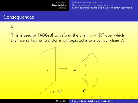
I.
This is used by [ABG70] to deform the chain x + iRd over whichthe inverse Fourier transform is integrated into a conical chain C.
x + i R Cd
Pemantle Hyperbolicity, stability and applications

OverviewHyperbolicity
Stability
Evolution of wavelike PDE’sRiesz kernel, and propagation in a coneMorse deformations and application to Taylor coefficients
application to multivariate generating functions
II.
Let us see how this was used in [BP11] to compute asymptotics ofthe Taylor series for
F (x , y , z) =1
(1− Z )(3− X − Y − Z − XY − XZ − YZ + 3XYZ )
=∑r
a(r , s, t)X rY sZ t (2)
where a(r , s, t) is the probability of the cube grove of orderr + s + t having a horizontal edge at barycentric coordinate (r , s, t).
Pemantle Hyperbolicity, stability and applications

OverviewHyperbolicity
Stability
Evolution of wavelike PDE’sRiesz kernel, and propagation in a coneMorse deformations and application to Taylor coefficients
Figure: a random cube grove of size 100Pemantle Hyperbolicity, stability and applications

OverviewHyperbolicity
Stability
Evolution of wavelike PDE’sRiesz kernel, and propagation in a coneMorse deformations and application to Taylor coefficients
Amoebas
To see how one applies the [ABG70] theory to rational generatingfunctions, we need one more definition. The amoeba of apolynomial q is the image of its zero set under the coordinatewiselog-modulus map
(z1, . . . , zd) 7→ (log |z1|, . . . , log |zd |) .The connected components of the complement of any amoeba areopen convex sets.
Pemantle Hyperbolicity, stability and applications

OverviewHyperbolicity
Stability
Evolution of wavelike PDE’sRiesz kernel, and propagation in a coneMorse deformations and application to Taylor coefficients
Cauchy’s integral formula
The method works for any rational function P/Q. Any Laurentexpansion of P/Q is convergent on some component B of thecomplement of amoeba(Q) and its coefficients are given there byCauchy’s formula, where x is any point in B:
arst = (2πi)−3
∫x+iT d
e−r ·z f (z) dz . (3)
Here we have changed to logarithmic coordinates, sof (z) := F (ez1 , . . . , ezd ) and T d := (R/2πZ)d .
Pemantle Hyperbolicity, stability and applications
OverviewHyperbolicity
Stability
Evolution of wavelike PDE’sRiesz kernel, and propagation in a coneMorse deformations and application to Taylor coefficients
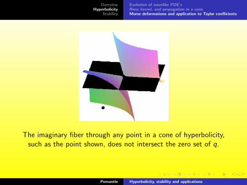
The imaginary fiber through any point in a cone of hyperbolicity,such as the point shown, does not intersect the zero set of q.
Pemantle Hyperbolicity, stability and applications

OverviewHyperbolicity
Stability
Evolution of wavelike PDE’sRiesz kernel, and propagation in a coneMorse deformations and application to Taylor coefficients
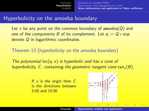
Hyperbolicity on the amoeba boundary
Let x be any point on the common boundary of amoeba(Q) andone of the components B of its complement. Let q := Q ◦ expdenote Q in logarithmic coordinates.
Theorem 13 (hyperbolicity on the amoeba boundary)
The polynomial loc(q, x) is hyperbolic and has a cone ofhyperbolicity, C , containing the geometric tangent cone tanx(B).
If x is the origin then Cis the directions between5:00 and 10:00
Pemantle Hyperbolicity, stability and applications

OverviewHyperbolicity
Stability
Evolution of wavelike PDE’sRiesz kernel, and propagation in a coneMorse deformations and application to Taylor coefficients
Hyperbolicity on the amoeba boundary
Let x be any point on the common boundary of amoeba(Q) andone of the components B of its complement. Let q := Q ◦ expdenote Q in logarithmic coordinates.
Theorem 13 (hyperbolicity on the amoeba boundary)
The polynomial loc(q, x) is hyperbolic and has a cone ofhyperbolicity, C , containing the geometric tangent cone tanx(B).
If x is the origin then Cis the directions between5:00 and 10:00
Pemantle Hyperbolicity, stability and applications

OverviewHyperbolicity
Stability
Evolution of wavelike PDE’sRiesz kernel, and propagation in a coneMorse deformations and application to Taylor coefficients
projective integral
It follows that the integral computing arst can be pushed onto acone pointing outward from x .
By the apparatus in [ABG70], one then has
ar ∼ E (r), E (r) =
(1
Q
),
where 1Q is the inverse Fourier transform of 1/q, otherwise known
as the fundamental solution to the wave equation DqE = δ.
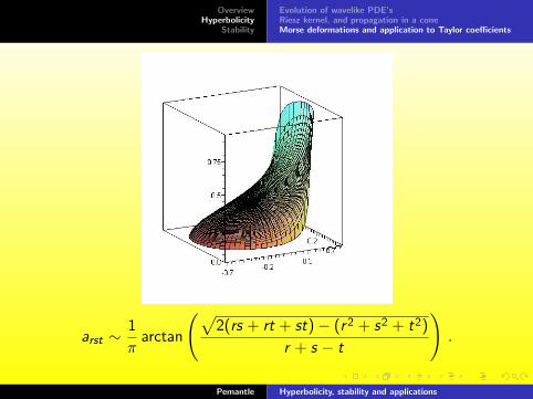
When Q is the denominator of (2), this gives
arst ∼1
πarctan
(√2(rs + rt + st)− (r 2 + s2 + t2)
r + s − t
).
Pemantle Hyperbolicity, stability and applications

OverviewHyperbolicity
Stability
Evolution of wavelike PDE’sRiesz kernel, and propagation in a coneMorse deformations and application to Taylor coefficients
projective integral
It follows that the integral computing arst can be pushed onto acone pointing outward from x .
By the apparatus in [ABG70], one then has
ar ∼ E (r), E (r) =
(1
Q
),
where 1Q is the inverse Fourier transform of 1/q, otherwise known
as the fundamental solution to the wave equation DqE = δ.
When Q is the denominator of (2), this gives
arst ∼1
πarctan
(√2(rs + rt + st)− (r 2 + s2 + t2)
r + s − t
).
Pemantle Hyperbolicity, stability and applications
OverviewHyperbolicity
Stability
Evolution of wavelike PDE’sRiesz kernel, and propagation in a coneMorse deformations and application to Taylor coefficients
arst ∼1
πarctan
(√2(rs + rt + st)− (r 2 + s2 + t2)
r + s − t
).
Pemantle Hyperbolicity, stability and applications

OverviewHyperbolicity
Stability
Evolution of wavelike PDE’sRiesz kernel, and propagation in a coneMorse deformations and application to Taylor coefficients
END PART I
Pemantle Hyperbolicity, stability and applications

OverviewHyperbolicity
Stability
Univariate stable functionsMultivariate stable functionsNegative dependenceStrong Rayleigh property
II: Applications of stability in probability andcombinatorics
Robin Pemantle
Current Developments in Mathematics, 18 November 2011
Pemantle Hyperbolicity, stability and applications

OverviewHyperbolicity
Stability
Univariate stable functionsMultivariate stable functionsNegative dependenceStrong Rayleigh property
Outline
I Univariate stable functions
II Multivariate stable functions
III Negatively dependent random variables
IV Multi-affine stability / strong Rayleigh property
Plan: go through I and II catalogue style: many statements, fewproofs, and hitting highlights rather than results that build on eachother. Then, for III and IV, try to give a coherent development.
Pemantle Hyperbolicity, stability and applications

OverviewHyperbolicity
Stability
Univariate stable functionsMultivariate stable functionsNegative dependenceStrong Rayleigh property
Univariate stable functions
Pemantle Hyperbolicity, stability and applications

OverviewHyperbolicity
Stability
Univariate stable functionsMultivariate stable functionsNegative dependenceStrong Rayleigh property
Real roots
A univariate stable polynomial f is by definition one with no rootsin the open upper half plane.
If f is real, then the set of roots is invariant under conjugation, so fhas no roots in the lower half plane either, hence has all real roots.
If, additionally, the coefficients of f are nonnegative, then all rootsof f are in (−∞, 0]. Polynomials whose roots are all real andnonpositive have useful properties. Let us denote this class ofunivariate polynomials by RR.
Pemantle Hyperbolicity, stability and applications

OverviewHyperbolicity
Stability
Univariate stable functionsMultivariate stable functionsNegative dependenceStrong Rayleigh property
Proposition 14
If f ∈ RR then f /f (1) is the probability generating function for asum of independent Bernoulli random variables. �
Proposition 15 (Polya frequency criterion, Edrei 1953)
A polynomial with nonnegative real coefficients is in RR if and onlyif its sequence of coefficients (a0, . . . , ad) is a Polya frequencysequence, meaning that all the minors of the matrix (an−k) havenonnegative determinant.
Corollary 16 (log-concavity)
The coefficient sequence of any polynomial in RR is log-concave. �
Pemantle Hyperbolicity, stability and applications

OverviewHyperbolicity
Stability
Univariate stable functionsMultivariate stable functionsNegative dependenceStrong Rayleigh property
Ultra-log concavity
In fact the coefficients of any f ∈ RR are ultra-logconcave,meaning that {ak/
(dk
)} is log-concave. These inequalities are due
to Newton (1707).
Perhaps the single most useful theorem about the class of(complex) stable polynomials is that it is closed undercoefficient-wise multiplication by Polya-Schur multipliersequences. Say that a sequence {λ(0), λ(1), . . .} is a multipliersequence if
f =∞∑n=0
anxn ∈ RR implies T (f ) :=∞∑n=0
λ(n)anxn ∈ RR .
Pemantle Hyperbolicity, stability and applications

OverviewHyperbolicity
Stability
Univariate stable functionsMultivariate stable functionsNegative dependenceStrong Rayleigh property
Polya-Schur Theorem
Theorem 17 (Polya-Schur, 1914)
Let φ(z) :=∑
n λ(n)zn/n! be the exponential generating functionfor the sequence λ. The following are equivalent.
(i) λ is a multiplier sequence.
(ii) φ is entire and either φ(z) or φ(−z) is the uniform limit oncompact sets of polynomials in RR.
(iii) Either φ(z) or φ(−z) is entire and can be written asCzneaz
∏∞k=1(1 + αkz) for a summable sequence of
nonnegative numbers {αk}.(iv) For all integers n > 0, the polynomial T [(1 + z)n] is
hyperbolic with zeros all of the same sign.
�Pemantle Hyperbolicity, stability and applications

OverviewHyperbolicity
Stability
Univariate stable functionsMultivariate stable functionsNegative dependenceStrong Rayleigh property
Multivariate stability
Multivariate stability
The presentation owes a debt to David Wagner’s recent surveyarticle in the AMS Bulletin [Wag11].
Definition 18
Recall: a complex polynomial q in d variables is said to be stableif q(z1, . . . , zd) = 0 implies not all coordinates zj are in the openupper half plane.
Pemantle Hyperbolicity, stability and applications

OverviewHyperbolicity
Stability
Univariate stable functionsMultivariate stable functionsNegative dependenceStrong Rayleigh property
Multivariate stability
Multivariate stability
The presentation owes a debt to David Wagner’s recent surveyarticle in the AMS Bulletin [Wag11].
Definition 18
Recall: a complex polynomial q in d variables is said to be stableif q(z1, . . . , zd) = 0 implies not all coordinates zj are in the openupper half plane.
Pemantle Hyperbolicity, stability and applications

OverviewHyperbolicity
Stability
Univariate stable functionsMultivariate stable functionsNegative dependenceStrong Rayleigh property
Easy properties
Proposition 19 (easy closure properties)
The class of stable polynomials is closed under the following.
(a) Products: f and g are stable implies fg is stable;
(b) Index permutations: f is stable implies f (xπ(1), ..., xπ(d)) isstable where π ∈ Sd ;
(c) Diagonalization: f is stable implies f (x1, x1, x3, . . . , xd) isstable;
(d) Specialization: if f is stable and Im (a) ≥ 0 thenf (a, x2, . . . , xd) is stable;
(e) Inversion: if the degree of x1 in f is m and f is stable thenxm
1 f (−1/x1, x2, . . . , xd) is stable;
�
Pemantle Hyperbolicity, stability and applications

OverviewHyperbolicity
Stability
Univariate stable functionsMultivariate stable functionsNegative dependenceStrong Rayleigh property
Easy properties
Proposition 19 (easy closure properties)
The class of stable polynomials is closed under the following.
(a) Products: f and g are stable implies fg is stable;
(b) Index permutations: f is stable implies f (xπ(1), ..., xπ(d)) isstable where π ∈ Sd ;
(c) Diagonalization: f is stable implies f (x1, x1, x3, . . . , xd) isstable;
(d) Specialization: if f is stable and Im (a) ≥ 0 thenf (a, x2, . . . , xd) is stable;
(e) Inversion: if the degree of x1 in f is m and f is stable thenxm
1 f (−1/x1, x2, . . . , xd) is stable;
�Pemantle Hyperbolicity, stability and applications

OverviewHyperbolicity
Stability
Univariate stable functionsMultivariate stable functionsNegative dependenceStrong Rayleigh property
Differentiation
Lemma 20 (differentiation)
If f is stable then ∂f /∂xj is either stable or identically zero.
Proof: Fix any values of {xi : i 6= j} in the upper half plane. Asa function of xj , f has no zeros in the upper half plane. By theGauss-Lucas theorem, the zeros of f ′ are in the convex hull,therefore not in the upper half plane. �
The next property, Wagner calls an “astounding” recentgeneralization of the Polya-Schur theorem.
Pemantle Hyperbolicity, stability and applications

OverviewHyperbolicity
Stability
Univariate stable functionsMultivariate stable functionsNegative dependenceStrong Rayleigh property
Multivariate Polya-Schur theorem
This characterizes not just multiplier sequence but all C-linearmaps preserving stability. To restrict to multiplier sequences, takeT (xα) = λ(α)xα.
Theorem 21 ([BB09, Theorem 1.3])
The C-linear map T : C[x ]→ C[x ] preserves stable polynomials ifand only if either its range is scalar multiples of a single stablepolynomial or the series∑
α∈(Z+)d
(−1)|α|T (xα)yα
α!
is a uniform limit on compact sets of stable polynomials in C[x , y ].
Pemantle Hyperbolicity, stability and applications

OverviewHyperbolicity
Stability
Univariate stable functionsMultivariate stable functionsNegative dependenceStrong Rayleigh property
What you are missing, part IV: any hint ofthe proof
The crucial step is to establish a criterion reminiscent tocriterion (iv) in the univariate case (that T [(1 + z)n] always hasreal roots of the same sign):
A power series∑
α Pα(x)yα whose coefficients arepolynomials in x is in the closure of stable polynomials inC[x , y ] if and only if for all β ∈ (Z+)d ,∑
α≤β(β)αPα(x)yα
is stable in C[x , y ].
Pemantle Hyperbolicity, stability and applications

OverviewHyperbolicity
Stability
Univariate stable functionsMultivariate stable functionsNegative dependenceStrong Rayleigh property
Determinants
A number of theorems and conjectures about stable polynomialshave to do with determinants. I will describe one classical result,one recent result and one conjecture that is still open.
1 Stability of det(A + x1B1 + · · ·+ xdBd).
2 Real roots of the mixed determinant det(xA,−B).
3 Nonnegative coefficients of the polynomial λ 7→ Tr(A + λB)n.
Pemantle Hyperbolicity, stability and applications

OverviewHyperbolicity
Stability
Univariate stable functionsMultivariate stable functionsNegative dependenceStrong Rayleigh property
Positive definite matrices
1.
A classical example of hyperbolicity already cited in [Gar51] that ifA is Hermitian and B is nonnegative definite then t 7→ det(A + tB)has only real zeros.
The multivariate generalization of this is that if A is Hermitian andB1, . . . ,Bd are positive definite, then
f := det(A + x1B1 + · · ·+ xdBd) (4)
is a real stable polynomial in x1, . . . , xd . Note: if A is also positivedefinite, then f has positive coefficients.
Pemantle Hyperbolicity, stability and applications

OverviewHyperbolicity
Stability
Univariate stable functionsMultivariate stable functionsNegative dependenceStrong Rayleigh property
Easy proof
The proof is more or less the same as the proof of hyperbolicity ofdet(A + tB).
Fix the real part of x1, . . . , xd , all positive, and remove a factor ofthe positive definite square root of Q :=
∑Re {xj}Bj on both the
right and the left to obtain det Q det(iI + H) where H is Hermitian(subsuming Q−1/2AQ−1/2 as well as the similar term with Areplaced by the sum of Im {xi}Bi . The eigenvalues of H are real,hence cannot equal −i . �
Pemantle Hyperbolicity, stability and applications
OverviewHyperbolicity
Stability
Univariate stable functionsMultivariate stable functionsNegative dependenceStrong Rayleigh property
Mixed determinants
2.
If A and B are n × n matrices, define the mixed determinant
det(A,B) :=∑S⊆[n]
det(A|S) det(B|Sc ) .
The definition for k matrices instead of two is analogous,substituting a partition into k parts for {S , Sc}.
Conjecture (Johnson’s conjecture)
If A is Hermitian and B is positive definite then det(xB,−A) hasonly real roots.
This (and much more) was recently proved by Borcea andBranden [BB08].
Pemantle Hyperbolicity, stability and applications
OverviewHyperbolicity
Stability
Univariate stable functionsMultivariate stable functionsNegative dependenceStrong Rayleigh property
BMV conjecture
3.
Conjecture (Bessis-Moussa-Villani 1975)
If A is Hermitian and B is nonnegative definite thenλ→ Tr(exp(A− λB)) is the Laplace transform of a positivemeasure on [0,∞).
This has been proved for 2× 2 matrices but is still open for allsizes greater than 2. This was shown in 2004 to be equivalent tothe following.
For all nonnegative definite matrices A and B and allintegers n > 0, the polynomial λ 7→ Tr(A + λB)n hasnonnegative coefficients.
Pemantle Hyperbolicity, stability and applications

OverviewHyperbolicity
Stability
Univariate stable functionsMultivariate stable functionsNegative dependenceStrong Rayleigh property
Negative dependence
Negatively dependent random variables
Pemantle Hyperbolicity, stability and applications

OverviewHyperbolicity
Stability
Univariate stable functionsMultivariate stable functionsNegative dependenceStrong Rayleigh property
Binary-valued random variables
Let Bn := {0, 1}n denote the Boolean lattice of rank n. The jointlaw of n binary random variables is a measure µ on Bn. Theprobability generating function f = fµ is given by
fµ(x1, . . . , xn) :=∑ω∈Bn
µ(ω)n∏
j=1
xωj
j = Exω .
Probability generating functions for measures on Bn all share twoproperties: they are multi-affine, meaning that no variableappears with a power greater than one, and their coefficients arereal and nonnegative.
Pemantle Hyperbolicity, stability and applications

OverviewHyperbolicity
Stability
Univariate stable functionsMultivariate stable functionsNegative dependenceStrong Rayleigh property
Negative correlation
Example 22 (n=2)
The function f (x , y) := p2xy + p(1− p)x + p(1− p)y + (1− p)2
generates two IID coin flips with success probability p. Thefunction f (x , y) + a(xy − x − y + 1) generates two exchangeablep-coins that are positively correlated if a < 0 and negativelycorrelated if a > 0.
(1−p)
2
2
p(1−p)
− a
− a
pp
(1−p)
2
2
p(1−p)p(1−p) + ap(1−p) + a
Pemantle Hyperbolicity, stability and applications
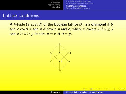
OverviewHyperbolicity
Stability
Univariate stable functionsMultivariate stable functionsNegative dependenceStrong Rayleigh property
Lattice conditions
A 4-tuple (a, b, c , d) of the Boolean lattice Bn is a diamond if band c cover a and if d covers b and c , where x covers y if x ≥ yand x ≥ u ≥ y implies u = x or u = y .
b c
d
a
Say that µ satisfies the positive lattice condition ifµ(b)µ(c) ≤ µ(a)µ(d) for every diamond (a, b, c , d). The reverseinequality is called the negative lattice condition.
Pemantle Hyperbolicity, stability and applications

OverviewHyperbolicity
Stability
Univariate stable functionsMultivariate stable functionsNegative dependenceStrong Rayleigh property
FKG
The positive lattice condition is very useful, due to the followingresult.
Theorem 23 (FKG)
If µ satisfies the positive lattice condition then µ is positivelyassociated and the projection of µ to any smaller set of variablessatisfies both these conditions as well.
Here, positively associated means that
Eµfg ≥ (Eµf ) (Eµg)
whenever f and g are both monotone increasing on µn.
Pemantle Hyperbolicity, stability and applications

OverviewHyperbolicity
Stability
Univariate stable functionsMultivariate stable functionsNegative dependenceStrong Rayleigh property
Negative association
Every function is positively correlated with itself. Thus, to definenegative association, we need to do more than reverse theinequality.
We say that µ is negatively associated if Eµfg ≤ (Eµf )(Eµg)whenever f and g are monotone increasing on Bn and in additionthere is a set S ⊆ {1, . . . , n} such that f depends only on{ωj : j ∈ S} and g depends only on {ωj : j /∈ S}.
Historically, a number of notions of negative dependence have beendefined. The weakest is pairwise negative correlation. Negativeassociation is the strongest one that was suspected to hold inmany examples.
Pemantle Hyperbolicity, stability and applications

OverviewHyperbolicity
Stability
Univariate stable functionsMultivariate stable functionsNegative dependenceStrong Rayleigh property
In search of a theory
Unfortunately, the negative lattice condition does not implynegative association. In fact the NLC is not closed under passingto subsets.
Up until [BBL09] there was no satisfactory theory of negativedependence. The paper [Pem00] attempted, but failed, to findone. Say that µ has property h-NLC+ if every measure obtainedfrom µ by ignoring a subset of the variables or applying an externalfield has the NLC. Here an external field means multiplying eachµ(ω) by
∏j λ
ωj
j and renormalizing.
Conjecture ([Pem00])
h-NLC+ implies negative association.
Pemantle Hyperbolicity, stability and applications

OverviewHyperbolicity
Stability
Univariate stable functionsMultivariate stable functionsNegative dependenceStrong Rayleigh property
Theory found!
It turns out that the “right” condition is not h-NLC+. Say that themeasure µ on Bn is strong Rayleigh if its generating functionf = fµ is stable.
Theorem 24 ([BBL09])
If µ is strong Rayleigh then µ is negatively associated.
In a short while I will give some indication of how this is proved.
Pemantle Hyperbolicity, stability and applications
OverviewHyperbolicity
Stability
Univariate stable functionsMultivariate stable functionsNegative dependenceStrong Rayleigh property
More about strong Rayleigh measures
Strong Rayleigh measures have more nice properties. For example,they are closed under partial symmetrization.
Let µij denote µ with the indices i and j transposed. If µ is SRthen for any i , j and any θ ∈ [0, 1] the measure θµ+ (1− θ)µij isSR. This is [BBL09, Theorem 4.20] and it leads to the very niceresult:
Theorem 25 (exclusion dynamics)
Begin with a configuration in Bn. For each i , j , swap the values ωi
and ωj at some rate βij . Then the law of the configuration at anytime t is SR.
Pemantle Hyperbolicity, stability and applications

OverviewHyperbolicity
Stability
Univariate stable functionsMultivariate stable functionsNegative dependenceStrong Rayleigh property
Nearest neighbor exclusion process on Z
−3 −2 1 2 4−1 3
time
−3−2 −1 1 0 32
Pemantle Hyperbolicity, stability and applications

OverviewHyperbolicity
Stability
Univariate stable functionsMultivariate stable functionsNegative dependenceStrong Rayleigh property
Complex geometry
I will not be proving these two results, but I will quote the authorsas to one aspect the methodology.
Clearly [this result] is real stable in nature. However, inorder to establish it, we have to consider the (wider)complex stable context.
In fact, they prove that stability of fµ implies stability offθµ+(1−θ)µij when µ is any complex-valued measure. It is importantthat f be multi-affine, but evidently not that f be real.
Pemantle Hyperbolicity, stability and applications

OverviewHyperbolicity
Stability
Univariate stable functionsMultivariate stable functionsNegative dependenceStrong Rayleigh property
Another case of extending beyond R+
The property h-NLC+ turns out to be equivalent to the (ordinary)Rayleigh property defined as the following inequality for all positivevectors x :
∀i , j∂f
∂xi(x)
∂f
∂xj(x) ≥ f (x)
∂2f
∂xi∂xj(x) . (5)
For multi-affine real polynomials, stability is equivalent to (5) forall x ∈ Rn. Thus SR differs from h=NLC+ in that the inequality isrequired for all x rather than for positive x . This should perhapsbe called h-NLC± because it is h-NLC with closure under externalfields both positive and negative!
Pemantle Hyperbolicity, stability and applications

OverviewHyperbolicity
Stability
Univariate stable functionsMultivariate stable functionsNegative dependenceStrong Rayleigh property
Multi-affine stable functions
The theory of multi-affine stable functions
Pemantle Hyperbolicity, stability and applications
OverviewHyperbolicity
Stability
Univariate stable functionsMultivariate stable functionsNegative dependenceStrong Rayleigh property
Polarization
Let f be a polynomial of degree m in one variable and define thepolarization of f to be the result of replacing x j be the normalizedelementary symmetric function
(mj
)−1ej(x1, . . . , xm). If f is a
probability generating function then the event {X = j} has beenreplaced by the event {
∑m1=1 X1 = j}.
Lemma 26 (polarization)
1. If f is univariate stable then its polarization is stable.
2. If f is multivariate stable then the analogous polarization,replacing x j
i in each monomial by ej(xi1, . . . , xi`), is stable.
(In fact part 1 is if and only if)
Pemantle Hyperbolicity, stability and applications

OverviewHyperbolicity
Stability
Univariate stable functionsMultivariate stable functionsNegative dependenceStrong Rayleigh property
Symmetric homogenization
The polarization lemma is proved via the classicalGrace-Walsh-SzegHo coincidence theorem.
It is then used by [BBL09] to prove the following result.
Suppose µ is a measure on Bn and define the symmetrichomogenization µsh of µ to be the measure on µ2n that issymmetric on xd+1, . . . , x2n, restricts to µ when x1, . . . , xn are setequal to 1, and is n-homogeneous. In other words, to pick fromµsh, first sample X1, . . . ,Xn from µ, then if these sum to k, choosen − k indices uniformly from n + 1 to 2n, set those variables equalto 1 and the rest of Xn+1, . . . ,X2n to zero.
Pemantle Hyperbolicity, stability and applications
OverviewHyperbolicity
Stability
Univariate stable functionsMultivariate stable functionsNegative dependenceStrong Rayleigh property
sh preserves SR
Lemma 27
If µ is strongly Rayleigh then so is µsh.
Proof: First one shows that the usual homogenization of apolynomial, multiplying each monomial by an appropriate power ofxd+1, preserves stability. This follows from facts abouthyperbolicity found in Garding’s original paper. Denoting thishomogenization by µ∗, we see that µsh is the polarization of µ∗, sothe result follows from the Polarization lemma. �
Pemantle Hyperbolicity, stability and applications

OverviewHyperbolicity
Stability
Univariate stable functionsMultivariate stable functionsNegative dependenceStrong Rayleigh property
sh preserves SR
Lemma 27
If µ is strongly Rayleigh then so is µsh.
Proof:
First one shows that the usual homogenization of apolynomial, multiplying each monomial by an appropriate power ofxd+1, preserves stability. This follows from facts abouthyperbolicity found in Garding’s original paper. Denoting thishomogenization by µ∗, we see that µsh is the polarization of µ∗, sothe result follows from the Polarization lemma. �
Pemantle Hyperbolicity, stability and applications

OverviewHyperbolicity
Stability
Univariate stable functionsMultivariate stable functionsNegative dependenceStrong Rayleigh property
sh preserves SR
Lemma 27
If µ is strongly Rayleigh then so is µsh.
Proof: First one shows that the usual homogenization of apolynomial, multiplying each monomial by an appropriate power ofxd+1, preserves stability.
This follows from facts abouthyperbolicity found in Garding’s original paper. Denoting thishomogenization by µ∗, we see that µsh is the polarization of µ∗, sothe result follows from the Polarization lemma. �
Pemantle Hyperbolicity, stability and applications
OverviewHyperbolicity
Stability
Univariate stable functionsMultivariate stable functionsNegative dependenceStrong Rayleigh property
sh preserves SR
Lemma 27
If µ is strongly Rayleigh then so is µsh.
Proof: First one shows that the usual homogenization of apolynomial, multiplying each monomial by an appropriate power ofxd+1, preserves stability. This follows from facts abouthyperbolicity found in Garding’s original paper.
Denoting thishomogenization by µ∗, we see that µsh is the polarization of µ∗, sothe result follows from the Polarization lemma. �
Pemantle Hyperbolicity, stability and applications

OverviewHyperbolicity
Stability
Univariate stable functionsMultivariate stable functionsNegative dependenceStrong Rayleigh property
sh preserves SR
Lemma 27
If µ is strongly Rayleigh then so is µsh.
Proof: First one shows that the usual homogenization of apolynomial, multiplying each monomial by an appropriate power ofxd+1, preserves stability. This follows from facts abouthyperbolicity found in Garding’s original paper. Denoting thishomogenization by µ∗, we see that µsh is the polarization of µ∗, sothe result follows from the Polarization lemma. �
Pemantle Hyperbolicity, stability and applications

OverviewHyperbolicity
Stability
Univariate stable functionsMultivariate stable functionsNegative dependenceStrong Rayleigh property
SR implies NA
Proof that strong Rayleigh measures are negativelyassociated:
1. Pass to µsh.
2. Observe that SR implies Rayleigh which implies pairwisenegative correlation.
3. The original proof by Feder and Mihail [FM92] of negativeassociation for balanced matroids now goes through, withhomogeneity of µsh providing the “balance” property.
�
Pemantle Hyperbolicity, stability and applications

OverviewHyperbolicity
Stability
Univariate stable functionsMultivariate stable functionsNegative dependenceStrong Rayleigh property
M. Atiyah, R. Bott, and L. Garding.
Lacunas for hyperbolic differential operators with constantcoefficients, I.
Acta Mathematica, 124:109–189, 1970.
J. Borcea and P. Branden.
Applications of stable polynomials to mixed determinants.
Duke J. Math., 143:205–223, 2008.
J. Borcea and P. Branden.
The Lee-Yang and Polya-Schur programs, I: linear operatorspreserving stability.
Invent. Math., 177:541–569, 2009.
J. Borcea, P. Branden, and T. Liggett.
Negative dependence and the geometry of polynomials.
J. AMS, 22:521–567, 2009.Pemantle Hyperbolicity, stability and applications

OverviewHyperbolicity
Stability
Univariate stable functionsMultivariate stable functionsNegative dependenceStrong Rayleigh property
Y. Baryshnikov and R. Pemantle.
Asymptotics of multivariate sequences, part iii: quadratic points.
Adv. Math., 228:3127–3206, 2011.
T. Feder and M. Mihail.
Balanced matroids.
Annual ACM Symposium on Theory of Computing, pages 26–38,1992.
L. Garding.
Linear hyperbolic partial differential equations with constantcoefficients.
Acta Math., 85:1–62, 1951.
R. Pemantle.
Toward a theory of negative dependence.
J. Math. Phys., 41:1371–1390, 2000.Pemantle Hyperbolicity, stability and applications

OverviewHyperbolicity
Stability
Univariate stable functionsMultivariate stable functionsNegative dependenceStrong Rayleigh property
David G. Wagner.
Multivariate stable polynomials: theory and application.
Bull. AMS, 48:53–84, 2011.
Pemantle Hyperbolicity, stability and applications