structural properties of scale-free networks

Structural Properties of Scale-FreeNetworks

Reuven Cohen, Shlomo Havlin, and Daniel ben-Avraham

WILEY-VCH Verlag Berlin GmbHAugust 18, 2002

1 Structural Properties of Scale-Free Networks

Reuven Cohen and Shlomo Havlin

Minerva Center and Department of Physics,Bar-Ilan University, Ramat-Gan, Israel

Daniel ben-Avraham

Physics Department and Center for Statistical Physics (CISP),Clarkson University, Potsdam NY 13699-5820, USA

Abstract

Many networks have been reported recently to follow a scale-free degree distribution in whichthe fraction of sites having

�connections follows a power law: �� . In this chapter

we study the structural properties of such networks. We show that the average distance be-tween sites in scale-free networks is much smaller than that in regular random networks, andbears an interesting dependence on the degree exponent � . We study percolation in scale-freenetworks and show that in the regime �� the networks are resilient to random break-down and the percolation transition occurs only in the limit of extreme dilution. On the otherhand, attack of the most highly connected nodes easily disrupts the nets. We compute the per-colation critical exponents and find that percolation in scale-free networks is non-universal,i.e. depends on � and different from the mean-field behavior in dimensions �� . Finally, wesuggest a novel and efficient method for immunization against the spread of diseases in socialnetworks, or the spread of viruses and worms in computer networks.

1.1 Introduction

1.1.1 Random graphs

Graph theory is rooted in the 18th century beginning with the work of Euler. A graph in itsmathematical definition is a pair of sets �� , where � is a set of vertices (the nodes of thegraph), and � is a set of edges, denoting the links between the vertices. In a directed graph,the edges are taken as ordered pairs, i.e., each edge is directed from the first to the secondvertex of the pair.

The work on graph theory has mainly dealt with the properties of special graphs. In the1960s, Paul Erdos and Alfred Renyi initiated the study of random graphs [1, 2, 3]. Randomgraph theory is, in fact, not the study of graphs (as there is no such thing as a “random graph”),but the study of an ensemble of graphs (or, as mathematicians prefer to call it, a probability

4 1 Structural Properties of Scale-Free Networks

space of graphs). The ensemble is a class consisting of many different graphs, where eachgraph has a probability attached to it. A property studied is said to exist with probability �if the total probability of all the graphs in the ensemble of having that property is � . Thisstructure allows the use of probability theory in conjunction with discrete mathematics for thestudy of graph ensembles.

Two well-studied graph ensembles are �� — the ensemble of all graphs having �vertices and � edges, and � �� — consisting of graphs with � vertices, where each possibleedge is realized with probability . These two families, initially studied by Erdos and Renyithemselves, are known to be similar if � �� , so long as is not too close to � or � [4],and are referred to as ER graphs. Examples of other well-studied ensembles are the family ofregular graphs, where all nodes have the same number of edges, �� , and the familyof unlabeled graphs, where graphs which are isomorphic under permutations of their nodesare considered the same object.

An important attribute of a graph is the average degree, i.e., the average number of edgesconnected to each node. We shall denote the degree of the � th node by

��and the average

degree by � �� . � -vertex graphs with � �� are called sparse graphs. In what follows,we concern ourselves exclusively with sparse graphs.

An interesting characteristic of the ensemble �� is that many of its properties have arelated threshold function, "! �#� � , such that if � "! the property exists with probability � , inthe “thermodynamic limit” of �%$'& , and with probability � if )(*+! . This phenomenonis similar to the physical notion of a phase transition. An example of such a property is theexistence of a giant component, i.e., a set of connected nodes, in the sense that a path existsbetween any two of them, whose size is proportional to � . Erdos and Renyi showed [2]that for ER graphs such a component exists if � �� (,� . If � �� -� only small componentsexist, and the size of the largest component is proportional to .0/1� . Exactly at the threshold,� �� , a component of size proportional to �

��243emerges. This phenomenon was described

by Erdos as the “double jump”. Another property is the average path length distance betweenany two sites, which in almost every graph of the ensemble is of order .0/1� .

1.1.2 Scale-free networks

The Erdos-Renyi model has been traditionally the dominant subject of study in the field ofrandom graphs. Recently, however, several studies of real world networks have indicated thatthe ER model fails to reproduce many of their observed properties.

One of the simplest properties of a network that can be measured directly is the degreedistribution, or the fraction �� of nodes having

�connections (degree

�). A well-known

result for ER networks is that the degree distribution is Poissonian, �� 65 �87:9��; �+<

, where9 � � �� is the average degree [4].Direct measurements of the degree distribution for networks of the Internet [5, 6], WWW

(where hypertext links constitute directed edges) [7, 8], e-mail network [9], citations of sci-entific articles [10], metabolic networks [11, 12], trust network [13], and many more, showthat the Poisson law does not apply. Rather, most often these nets exhibit a scale-free degreedistribution:

�� >= �@?0?A? �CB (1.1)

1.1 Introduction 5

where�� = �� is a normalization factor, and

=and B are the lower and upper

cutoffs for the connectivity of a node, respectively. The divergence of moments higher than� �� (as B�$ & when � $ & ) is responsible for many of the special properties attributedto scale-free networks.

All real-life networks are finite (and all their moments are finite). The actual value of thecutoff B plays an important role. It may be approximated by noting that the total probabilityof nodes with

� (*B is of order �;� [14, 15]:

�� ; � ? (1.2)

This yields the result

B �>= � �2� �� ? (1.3)

The degree distribution does not characterize the graph or ensemble in full. There areother quantities, such as the degree-degree correlation (between connected sites), the spatialcorrelations, etc. Several models have been presented for the evolution of scale-free networks,each of which may lead to a different ensemble. The first suggestion was the preferentialattachment model by Barabasi and Albert, which came to be known as the “Barabasi-albertmodel” [5] . Several variants have been suggested to this model (see, e.g., [16, 17]). In thisChapter we will concentrate on the “Molloy-Reed construction” [18, 19, 20], which ignoresthe evolution and assumes only the degree distribution and no correlations between nodes.Thus, the site reached by following a link is independent of the origin.

Scale-free distributions have been studied in physics, particularly in the context of fractalsand of Levy flights. Fractals are objects which appear similar (at least in some statistical sense)at every lengthscale [21, 22]. Many natural objects, such as mountains, clouds, coastlines andrivers, as well as the cardiovascular and nervous systems are known to be fractals. This iswhy we find it hard to distinguish between a photograph of a mountain and that of part of themountain, neither can we ascertain the altitude from which a picture of a coastline had beentaken. Diverse phenomena, such as the distribution of earthquakes, biological rhythms andrates of transport of data packets in communication networks, are also known to posses a scale-free distribution. They come in all sizes and rhythms, spanning many orders of magnitude.

Levy flights were suggested by Paul Levy [23], who was studying what is now knownas Levy stable distributions. The question he asked was, When is the length distribution ofa single step in a random walk similar to that of the entire walk? Besides the known result,that of the Gaussian distribution, Levy found an entire new family — essentially that of scale-free distributions. Stable distributions do not obey the central limit theorem (stating that forlarge numbers of steps the distribution of the total displacement tends to Gaussian), due to thedivergence of the variance of indivual steps. Levy walks have numerous applications [24, 25].An interesting observation is that animal foraging patterns which follow stable distributionshave been shown to be their most efficient strategy [26, 27]. For recent reviews on complexnetworks and in particular scale free networks see Refs. [28, 29].


1.2 Small and Ultra-Small Worlds

Regular lattices are embedded in Euclidean space, of a well-defined dimension, � . This meansthat � �� , the number of sites within a distance � from an origin, grows as � �� (forlarge � ). For fractal objects � in the last relation is non-integer and is replaced by the fractaldimension �� . Similarly, the chemical dimension, �� , is defined by the scaling of the number ofsites within

edges or less from a given site (an origin), � � � � ��

. A third dimension, �� ,relates between the chemical path (the shortest distance along edges) and Euclidean distances,�� . It satisfies ��

;� � [21, 22, 30].

An example of an object where these concepts fail is the Cayley tree (also known as theBethe lattice). The Cayley tree is a regular graph, of fixed degree

9, and no loops. It has been

studied by physicists in many contexts, since its simplicity often allows for exact analyses.An infinite Cayley tree cannot be embedded in a Euclidean space of finite dimensionality.The number of sites at

is � � �� 9 �� . Since the exponential growth is faster than any

power-law, Cayley trees are referred to as infinite-dimensional systems.

In most random network models the structure is locally tree-like (since most loops occuronly for � � �� ), and, since the number of sites grows as � � �� , they are alsoinfinite-dimensional. As a consequence, the diameter of such graphs (i.e., the minimal pathbetween the most distant nodes) scales like � � .0/1� [4]. This small diameter is to becontrasted with that of finite-dimensional lattices, where � � � � 2 �� .

Recently, a model has been suggested by Watts and Strogatz [31, 32] which retains thelocal high clustering of lattices while reducing the diameter to � � .A/1� . This, so called,small world network is achieved by replacing a fraction � of the links in a regular lattice withrandom links, to random distant neighbors. (In other variants of the small world model the“long range” links are simply added on, without prior removal of lattice links.) A study ofscale-free networks embedded in Euclidean space (at the obvious price of a cutoff in

�) which

exhibit finite dimensions can be found in [33].

1.2.1 Diameter of scale-free networks

We now aim to show that scale-free networks with degree exponent � � � � � possess adiameter � � .A/ .0/1� , smaller even than that of ER and small world networks. If the networkis fragmented, we will only be interested in the diameter of the largest cluster (assuming thereis one). Our analysis of the diameter of the Molloy-Reed scale-free networks is based on [34].

We adopt a different definition of diameter: the average distance between any two siteson the graph. We find it easier still to focus on the radius of a graph, �� #� : the averagedistance of all sites from the site of highest degree in the network (if there is more than one,we pick one arbitrarily). The diameter of the graph, � , is restricted to:

�� (1.4)

and thus essentially scales like � .

1.2 Small and Ultra-Small Worlds 7

1.2.2 Minimal graphs and lower bound

We begin by showing that the radius of any scale-free graph with � (� has a rigorous lowerbound that scales as .0/ .0/1� . It is easy to convince oneself that the smallest diameter of agraph, of a given degree distribution, is achieved by the following construction: Start with thehighest degree site, then connect to each successive layer the extant sites of highest degree,until the layer is full. By construction, loops will occur only in the last layer.

Let the number of links outgoing from theth shell (layer) be � � . Let B � denote the highest

degree of a site not yet reached by theth layer. Then, for the graph of minimal diameter

described above,

� � � � � �� = �� B � �� ? (1.5)

The number of links outgoing from layer�� equals the total number of links in all the sites

between B � and B �� minus one link for each site — the one used to connect to the previouslayer:

� �� *�

�� = �� B

� �� ? (1.6)

Solving these recursion relations, with the initial conditions B �� 2 � �� and � �

� B � ,leads to:

� � �� (1.7)

where� � � � � � � ; �� = , � � �� ; � � � � � , and

B � � = �� ;� �

�� ? (1.8)

To bound the radius � of the graph, we will assume that the low degree sites are connectedrandomly to the giant cluster. We pick a site of degree �� .A/1.0/1� � � 2� �� . UsingEq. (1.8) we can show that if

� � .0/ .A/1� ; .0/ �� then B � � � �� , so, with probability 1 allsites of degree

� � ��lie within

� layers from the site we picked. On the other hand, if westart uncovering the graph from any site — provided it belongs to the giant component — thenwithin a distance

�from this site there are at least

�bonds. The probability that none of those

bonds leads to our site (of degree��

) is � � � �� ; � �� . That is, if � ��

;� �� ,

at least one bond will lead to our site. Thus, taking�� .A/ .A/1� , we will definitely

reach a site of at least degree� �

in the �

th layer from almost any site. Since ��

,all sites are at a distance of order .0/ .A/1� from the highest degree site, and � � .0/ .A/1� is arigorous lower bound for the diameter of scale-free networks with � (�� .1.2.3 The general case of random scale-free networks

We now argue that the scaling of � � .0/ .A/1� is actually realized in the general case ofrandom scale-free graphs with �� . One can view the process of uncovering the


network as actually building it, by following the links one at a time. For simplicity, let us startwith the site of highest degree, B � � � 2� �� (guaranteed to belong to the giant component).Next, we expose the layers one at a time. We view the graph as built from one large developingcluster, and sites which have not yet been reached (they might or might not belong to the giantcomponent), see Fig. 1.1. A similar consideration has been used by Molloy and Reed [19].

After

layers are explored the distribution of the yet unreached sites changes (since mosthigh-degree sites are exposed first) to �� 5�� ; B � � [19].

Let us now consider layer � � . A threshold function emerges: the new distribution of

unvisited sites behaves like a step function — almost �� for� �*B �� , and � for

� (>B �� .The reason for this is as follows. A site with degree

�has a probability of � � ; �#�)� �� to

be reached by following a link1. If there are � � outgoing links then for �� ( � we canassume that, in the limit ��$ & , the site will be reached in the next level with probability 1.Therefore, all unvisited sites with degree

� ( �;� � will be surely reached in the next chemical

layer. On the other hand, almost all the unvisited sites with degree� �,�

;� � will remain

unvisited in the next layer and their distribution will remain virtually unchanged. From theseconsiderations, the highest degree of the unexplored sites in layer

�� is determined by:

B �� ; � � ? (1.9)

In layer � � all sites with degree

� ( �;� � will be exposed. Since the probability

of reaching a site via a link is proportional to� �� , the average degree of sites reached

by following a link is � � � �� ; � �� [14]. � for layer

can be computed from the general

formula [14], valid for scale-free distributions,

� � � � � �� B 3 � � = 3 ��

B� � � = � �� (1.10)

but with the layer cutoff B of (1.9). That is, � � � B 3 � �� .Using the above consideration, the number of outgoing links from layer

� � can becomputed. Consider the total degree of all sites reached in the

�� level. This includes allsites with degree

�, B �� *B � , as well as other sites with average degree proportional to� � � (the � � is due to one link going into the shell). Thus, the value of � (the avergae number

of links for a site reached via a link) is calculated using the cutoff B �� . (Loops within a layer,and multiple links connecting a site in layer

�� , can be neglected as long as the number ofsites in the layer is less than order � , � $ & .) The two contributions can be written as thesum of two terms:

� �� *� � �� B �� ? (1.11)

Noting that �� and that � � B 3 � [14], it follows that � �� B � � �� (note that

both terms in Eq. (1.11) scale similarly). This results in a second recurrence equation:

� �� B � �� (1.12)

where� � �� = �� 3 � = �

�.

1We assume that �� for the unvisited sites is fixed, since it is dominated by the low-degree nodes, whose distri-bution is unchanged.

1.2 Small and Ultra-Small Worlds 9

K

χ l

l

l

Figure 1.1: Illustration of the exposure process. The large circle denotes the exposed fraction of thegiant component, while the small circles denote individual sites. The sites on the right have not beenreached yet. After [34]

Solving the equations (1.9) and (1.12) yields

� � �� (1.13)

where � � is the number of outgoing links from theth layer. Eq. (1.9) then leads to:

B � �� ? (1.14)

Using the same considerations that follow Eq. (1.8), one can deduce that also here

� � .0/ .0/1� ? (1.15)

Our result that � � .A/ .0/1� is consistent with the observations that the distance in theInternet network is extremely small, and that the distance in metabolic scale-free networks isalmost independent of � [11].

For � ( � and � � � , � is independent of � , and since the second term of Eq. (1.11) isdominant, Eq. (1.11) reduces to � �� >� � � � , where � is a constant depending only on� . This leads to the known result � � �� #� � � � � �� and the radius of the network [35] is

� � .0/1� ? (1.16)

For � � � , Eq. (1.11) reduces to � �� .0/ � � . Taking the logarithm of this equationone obtains .A/ � �� .0/ � � � .0/ .A/ � � . Defining � �� .A/ � � one obtains a difference equationwhich may be approximated (in the continuum limit) by � � .0/ . Substituting � � .0/ , theequation reduces to

� ��

5 � � � � � ? (1.17)


The lower bound is obtained from the highest degree site for � � � , having degree B �=�� . Thus, � �

��=�� . The upper bound results from that

for which � � � � (and lowerorder corrections). The integral in Eq. (1.17) can be approximated by the steepest descentmethod, leading to

� � .0/1� ; � .0/ .0/1� � � (1.18)

(assuming .A/ .0/1� � � ).The result of Eq. (1.18) has been obtained rigorously for the maximum distance in the

Barabasi-Albert (BA) model [5], where � � � (for= � � ) [36]. Although the result in

[36] applies to the largest distance between two sites, their derivation leaves no doubt that theaverage distance would behave similarly. For

= � � , the graphs in the Barabasi-Albert modelturn into trees, and the behavior of � � .0/1� is obtained [36, 37]. It should be noted that for= � � the giant component in the random model contains only a fraction of the sites (whilefor= � � it contains all sites — at least to leading order). This might explain why exact trees

and BA trees are different from Molloy-Reed random graphs.

1.3 Percolation

Since the 1940s percolation has been the subject of intense studies among physicists andmathematicians. In site percolation, usually defined on lattices, the sites (nodes) are present(or occupied, or wet) with probability � , or equivalently, removed (blocked) with probability � � �� . The (infinite) network undergoes a sharp phase transition at a critical threshold �� ,from a connected, or percolating phase, where a spanning cluster runs across the entire size ofthe system, for ��(�� , to a fragmented phase, where only finite clusters exist, for � �� . Anintroduction to the general subject of percolation can be found in [38, 22, 30]2

The percolation transition is continuous (second order), and near the transition point manyproperties behave as power laws. For example, the probability for a site to be in the spanningcluster (for � (� � ) grows as � � � �� , and the number of clusters of size � , at� � �� , is �� . The critical exponents � , � , and their likes, are universal, dependingonly upon the dimensionality � of the lattice. For � � �� the lattice dimension no longerplays a significant role and the critical exponents assume their mean-field values (e.g., � � � ,� �� ; � ). The mean-field case can be conviniently obtained from the exact solution of thepercolation problem on Cayley trees (whose effective dimension is infinite). Percolation in ERgraphs also follows mean-field behavior. The percolation threshold is �� ; � 9 � � �for Cayley trees, and ��

;� �� for ER graphs.

The problem of percolation on scale-free networks has important practical applications.Below we explore consequences to the resilience of the Internet in the face of random break-down of servers as well as under intentional attack, and to immunization strategies against thespread of contagious epidemics in population and computer networks.

2We have exchanged here the traditional roles of � and � in percolation theory, �� , to conform with whatseems to be the norm in papers on scale-free graphs.

1.3 Percolation 11

1.3.1 Random breakdown

For a graph having degree distribution �� to have a spanning cluster, a site � which isreached by following a link (from site � on) the giant cluster must have at least one other link,on average, to allow the cluster to exist. For this to happen the average degree of site � mustbe at least � (one incoming and one outgoing link), given that site � is connected to � :

� � �� ? (1.19)

Using Bayes’ rule we get

�� ;��

;�� (1.20)

where �� C�� is the joint probability that node � has degree� �

and that it is connected tonode � . For randomly connected networks (neglecting loops) ��

;�� >� � and

�� ;�� , where � is the total number of nodes in the network. Using the

above criterion Eq. (1.19) reduces to [18, 14]:

� � � � � �� (1.21)

at the critical point. A spanning cluster exists for graphs with � ( � , while graphs with�� contain only small clusters whose size � is negligible compared to the entire network,.�� ; � � � . The criterion (1.21) and its range of validity was derived rigorously byMolloy and Reed [18], using somewhat different arguments.

Neglecting the loops is justified below the transition, since the probability for a bond toform a loop in an � -node cluster is proportional to � �

;� ��

(i.e., proportional to the probabilityof choosing two sites in that cluster). An estimate of the fraction of loops �� in the networkyields

� ��

��

� � (1.22)

where the sum is over all clusters in the system ( � � is the size of the � th cluster), and�

isthe size of the biggest cluster. Since

� � .A/1� below the transition, � �� is negligible when��$ & .

1.3.2 Percolation critical threshold

The above reasoning can be applied to the problem of percolation in a generalized randomnetwork [14]. If we randomly remove a fraction of the sites (along with the emanatinglinks), the degree distribution of the remaining sites will change. For instance, sites with initialdegree

�� will have, after the random removal of nodes, a different number of connections�

, depending on the number of removed neighbors. The initial degree distribution, � � ��,

becomes, following dilution

��

� �� ? (1.23)


The first two moments of the new �� are

� �� (1.24)

and

� ��

��

� � � � � �� (1.25)

where � � ��

and � ��

are computed with respect to the original distribution � � ��. On substi-

tuting the new moments in Eq. (1.21) we obtain the criterion for criticality, following dilution:

� � � � � �� ? (1.26)

This can be rearranged, to yield the critical threshold for percolation [14]:

� � �� (1.27)

where � � � � � �� ; � � � � is calculated using the original distribution, before the random removalof sites.

Eqs. (1.21) and (1.27) are applicable to random graphs of arbitrary degree distribution.For example, using (1.27) for Cayley trees yields the well-known threshold [38, 22] � � �� ; � 9 � � � . Another example is ER graphs. Their edges are distributed randomly andthe resulting degree distribution is Poissonian [4]. Applying the criterion from Eq. (1.21) tothe Poisson distribution of ER graphs yields

� � � � � ��

� �� (1.28)

which reduces to the known result [4] � �� .Evidently, the key parameter governing the threshold, according to (1.27), is the ratio of

second- to first-moment, � � . This may be estimated by approximating (1.1) to a continuousdistribution (the approximation becomes exact for � � = � B , and it preserves the essentialfeatures of the transition even for small

=):

� � � � � � �� B

3 �� = 3 � B� �� = � � ? (1.29)

In the limit of B � =, we have

� � $ ��

�� = � � ( � ;= � � B

3 � � � � � �� ;B � � � � � � .

(1.30)

1.3 Percolation 13

We see that for � ( � the ratio � � is finite and there is a percolation transition at � � � � � � � 3 = �>� �� : for ( � the spanning cluster is fragmented and the network is destroyed.However, for � �� the ratio � � diverges with B and so � $ � when B�$ & (or � $ & ).The percolation transition does not take place: a spanning cluster exists for arbitrarily largefractions of dilution, �%� . In finite systems a transition is always observed, though for�� the transition threshold is exceedingly high. For the case of the Internet ( � � � ; � ),we have � � � B � 24� � � � 243 . Considering the enormous size of the Internet, � ( � �� ,one needs to destroy over 99% of the nodes before the spanning cluster collapses. For � ( �calculation of � shows that it is lower than � even before the breakdown occurs. For � ( � and= � � the network consists of only finite clusters and no spanning cluster to begin with (thisis reminiscent of the result for � ( ��? �� ?0?A? found in [20], where the different threshold stemsfrom rigorous consideration of the discrete nature of (1.1)). Note that if

= � � , a spanningcluster exists for all values of � .

1.3.3 Generating functions

A general method for studying the size of the infinite cluster and the residual network for agraph with an arbitrary degree distribution was first found by Molloy and Reed [19]. Theyconsider the infinite cluster as it is being exposed, layer by layer, and develop differentialequations relating the number of unexposed links and unvisited sites in subsequent shells (seeSection 1.2).

An alternative, and very powerful approach based on generating functions was advancedby Newman, Watts and Strogatz [35]. Their method is beautifully reviewed in this book, inthe Chapter by Newman. Here, we follow closely in their footsteps. Our ultimate goal is tocompute the size of the giant component as well as the critical exponents associated with thepercolation transition in scale-free networs, resulting from random dilution (Section 1.3.5).

In [35, 39] a generating function is constructed for the degree distribution:

� � ��

�� ? (1.31)

The probability of reaching a site with degree�

by following a specific link is� ��

;� ��

[18, 14, 35], and its corresponding generating function is

� � � � � ��

� �� ; � �� ? (1.32)

Let � � � � � be the generating function for the probability of reaching a branch of a given sizeby following a link. When a fraction � � � � of the sites are diluted, � � satisfies theself-consistent equation:

� � � � � � � � � � � � � � �� ? (1.33)

Given that � � ��

is the generating function for the degree of a site, the generating functionfor the probability of a site to belong to an � -site cluster is:

� � �� ? (1.34)


Below the transition, all clusters are finite and � � � �� . However, above the transition

� � � ��

is no longer normalized, since it excludes the probability of the incipient infinite cluster,� � . In other words, � � � � � � � � � � . It follows that

� � � � ��

�� (1.35)

where � � � � � � � is the smallest positive root of

� ��

��

� �� ? (1.36)

This equation can be solved numerically and the solution can be substituted into Eq. (1.35)to compute the size of the infinite cluster in a random graph of arbitrary degree distribution.(The analysis neglects the presence of loops, which is well justified near criticality.)

1.3.4 Intentional attack

Another model of interest, suggested in [40], is that of intentional attack on the most highlyconnected nodes of the network. In this model an attacker (e.g., computer hackers trying tocause damage to the network, or doctors trying to disrupt a contagious epidemic) succeedsin knocking off a fraction of the most highly connected sites in the network. As might beexpected, such a strategy is far more effective than random dilution. We shall see, in fact, thata small threshold suffices to disrupt the net (for all � ).

Next we consider analytically the consequence of such an attack, or sabotage, on scale-freenetworks [41]. A different approach was given independently in [39]: (a) the cutoff degree Breduces to some new value

�B ��B , and (b) the degree distribution of the remaining sites isno longer scale-free, but is changed due to the removal of many of their links. Recall that theupper cutoff B , before the attack, may be estimated from

��

� ? (1.37)

Similarly, the new cutoff�B , after the attack, follows from

��

� ��

� ��

�� ? (1.38)

If the size of the system is large, � � �; , the original cutoff B may be safely ignored. We

can then obtain�B approximately by replacing the sum with an integral:

�B � = �2� � � � ? (1.39)

We estimate the impact of the attack on the distribution of the remaining sites as follows.The removal of a fraction of the sites with the highest degree results in a random removal of

1.3 Percolation 15

links from the remaining sites — links that had connected the removed sites with the remainingsites. The probability

� for a link to lead to a deleted site equals the ratio of the number oflinks belonging to deleted sites to the total number of links:

� � ��

� � �� (1.40)

where � � ��

is the initial average degree. With the usual continuous approximation, and ne-glecting B , this yields

� �� B = �

� �� 0� � � 2 � � � � � (1.41)

for �*( � . For � � � , �)$ � , since just a few nodes of very high degree control the entireconnectedness of the system. Indeed, consider a finite system of � sites and � � � . Theupper cutoff B � � must then be taken into account, and approximating Eq. (1.40) by anintegral yields

� � .A/ �� ; = �

. That is, for � � � , a very small value of is needed to destroyan arbitrarily large fraction of the links as ��$ & .

With the above results we can compute the effect of intentional attack, using the theorypreviously developed for random removal of sites [14]. Essentially, the network after attackis equivalent to a scale-free network with cutoff

�B , that has undergone random removal of afraction

� of its sites. Since the latter effect influences the probability distribution as describedin Eq. (1.23), the result in Eqs. (1.27) and (1.29) can be used, but with

� � � �B; = � � ��

and�B replacing �� and B , respectively. This yields the equation:

� �B; = � � ��

� � �= � � �B

; = � 3 �� *� �� (1.42)

which can be solved numerically to obtain�B � = � � � , and then � � = � � � can be retrieved from

Eq. (1.39). In Fig. 1.4 we plot � (there denoted��

) — the critical fraction of sites needed tobe removed in the sabotage strategy to disrupt the network — computed in this fashion, andcompared to results from numerical simulations. A phase transition exists (at a finite � ) forall � ( � . The decline in �� for large � is explained from the fact that as � increases thespanning cluster becomes smaller in size, even before attack. (Furthermore, for

= � � theoriginal network is disconnected for � large enough.) The decline in � as � $ � results fromthe critically high degree of just a few sites: their removal disrupts the whole network. Thiswas first argued in [40]. We note that for infinite systems � $ � as ��$ � . The criticalfraction �� is rather sensitive to the lower degree cutoff

=. For larger

=the networks are

more robust, though they still undergo a transition at a finite � . (Fig. 1.4 illustrates the caseof= � � .)

1.3.5 Critical exponents

The generating functions method has the advantage of turning a combinatorial problem intoan algebraic one, concerning power series. The algebraic problem is often simpler.


Here we use generating functions for obtaining the percolation critical exponents [42].These can be extracted from the resulting power series by means of appropriate Abelian andTauberian methods [43, 44].

First, we compute the order parameter critical exponent � . Near criticality the probabilityof belonging to the spanning cluster behaves as � � � � � �� . For infinite-dimensionalsystems (such as a Cayley tree) it is known that � � � [38, 22, 30]. This regular mean-fieldresult is not always valid, however, for scale-free networks. Eq. (1.35) has no special behaviorat � � �� ; the singular behavior comes from � . At criticality, � � � � and Eq. (1.35) implythat � � � . We therefore examine Eq. (1.36) for � � � �� and � � �� :

� �� )� ��

�� ? (1.43)

The sum in (1.43) has the asymptotic form��

� �� >� � � � � � � � ��

� ��

� �� (1.44)

where the highest-order analytic term is� �� , � �� . Using this in Eq. (1.43), with

�� ;� � �*� � � � �� ; � � � � � � �C� , we get

� � � � �*� � � ��

� � ��

3? (1.45)

The divergence of�

as � � � confirms the vanishing threshold for the phase transition in thatregime. Thus, limiting ourselves to � ( � , and keeping only the dominant term as � $ � ,Eq. (1.45) implies

� �� A� ��

�� ( � ?(1.46)

Returning to � � , Eq. (1.35), we see that the singular contribution in � is dominant only forthe irrelevant range of � �� . For � ( � , we find � � � �� .

We see that the order parameter exponent � attains its usual mean-field value only for� ( � . Moreover, for � � �

the percolation transition is higher than 2nd-order: for � � � ��

��

the transition is of the � th-order.For networks with � �� the transition still exists, though at a vanishing threshold, �� .

The sum in Eq. (1.43) becomes:

��

� �� ? (1.47)

1.3 Percolation 17

Using this in conjunction with Eq. (1.36), and remembering that here �� and therefore� �� , leads to

� ��

�� ? (1.48)

The results can be summarized by

� �� 3 �� 3 � �� ( � ?

(1.49)

In other words, the transition in � � �� is a mirror image of the transition in � � �� .

An important difference is that � � � � is not � -dependent in � � � � � , and the amplitudeof � � diverges as � $ � (but remains finite as � $ �

). Some of the results for � have beenreported before in [41], and also found independently in a different but related model of virusspreading [45, 46, 47]. The existence of an infinite-order phase transition at � � � for growingnetworks of the Albert-Barabasi model has been reported in [48, 49]. These examples suggestthat the critical exponents are not model-dependent but depend only on � .

In [35] it was shown that for a random graph of arbitrary degree distribution the finiteclusters (of size � ) follow the usual scaling form:

�� 5 � �2 �� ? (1.50)

At criticality � � � � � � � � � �� diverges and the tail of the distribution behaves as a powerlaw. We now derive the exponent � . The probability that a site belongs to an � -cluster is � � � �� , and is generated by � � :

� � �� ? (1.51)

The singular behavior of � � ��

stems from � � � �� , as can be seen from Eq. (1.34). � � � � �itself can be expanded from Eq. (1.33), by using the asymptotic form (1.44) of � � . We let

� �� , as before, but work at the critical point, � � �� . With the notation � �� ,we finally get (note that at criticality � � � � �� ):

� � � � � � � � � ��

� � � � � � � � � � � � � ��

� � ��

� ?(1.52)

¿From this relation we extract the singular behavior of � � : �� . Then, using Tauberian

theorems [43] it follows that � � � �� , hence � � � � .For � ( �

the term proportional to � ��

in (1.52) may be neglected. The linear term�� may be neglected as well, due to the factor � . This leads to � � � � 24� and to the usualmean-field result

� �� ( � ? (1.53)


For � � �, the terms proportional to �� , �

�may be neglected, leading to � � � � 2� � � � and

� � � � ��

� � �� ? (1.54)

Note that for � � � � � the percolation threshold is strictly �� . In that case we work at� � � small but fixed, taking the limit

� $ � at the very end. For the case � � � � � , � inEq. (1.54) represents the singularity of the distribution of branch sizes. For the distributionof cluster sizes in this range one has to consider the singularity of

�in Eq. (1.34), leading to

� � � .For growing networks of the Albert-Barabasi model with � � � , it has been shown that

� � � � � � .A/ � � ��

[49]. This is consistent with � � � plus a logarithmic correction. Relatedresults for scale-free trees have been presented in [50].

At the transition point the size of the largest cluster,�

, can be obtained from the finitecluster distribution by taking the integral over the tail of the distribution to equal �

;� . This

results in� � � � �� 2� �� ? (1.55)

For � � �this reduces to the known �

��2C3dependence [4]. For � $ � , � � � � 2C� . It is not

yet clear whether the results have a meaningful interpretation for � �� .The critical exponent � , for the cutoff cluster size, may be also derived directly. Finite-size

scaling arguments predict [38] that

�� & � � �� (1.56)

where � is the number of sites in the network, � is the correlation length critical exponent:� � �� , and � is the dimensionality of the embedding space. Using a continuousapproximation of the distribution (1.1) one obtains [14]

� � � � � �� B

3 � � = 3 �� B� � � = � �� (1.57)

where, as usual B � � � 2� �� . For � � � � �, this and Eq. (1.27) yield

� � � & � � � � �� B 3 �� (1.58)

which in conjunction with Eq. (1.56) leads to

�� ? (1.59)

For �>( �we recover the regular mean-field result �

� �;� . Note that Eqs. (1.56), (1.49),

(1.54) are consistent with the known scaling relation: � � � � � � [38, 22, 30]. For � �� ,� � � & �� and � � �#� � � B � 3 � � � � 3 � 2� �� . Therefore

�� (1.60)

again consistent with the scaling relation � � � � � � (cf Eq. (1.49)).

1.3 Percolation 19

1.3.6 Fractal dimension

It is well known that on a random network in the well connected regime, the average distancebetween sites is of order .�� [4, 51]. This has also been shown to hold for sgeneral net-works [35] and may be even lower for scale-free networks [34]. However, the diluted caseis essentially the same as infinite-dimensional percolation. In this case, there is no notion ofgeometrical distance (since the graph is not embedded in an Euclidean space), but only ofchemical distance (the smallest number of edges connecting any two nodes). It is known frominfinite-dimensional percolation theory that the fractal dimension at criticality is � � � � [22].Therefore the average (chemical) distance � � between pairs of sites on the spanning cluster atcriticality behaves as

� � � � � � (1.61)

where � is the number of sites in the spanning cluster. This is analogous to percolation infinite dimensions, where in lengthscales smaller than the correlation length the cluster is afractal with dimension � � and above the correlation length the cluster is homogeneous andhas the dimension of the embedding space. In our infinite-dimensional case, the crossoverbetween these two behaviors occurs around the correlation length

� � � � � � �� .For ��

the situation is somewhat different. Below the transition all clusters arefinite and almost all finite clusters are trees. The correlation length can be defined using theformula [22]:

��

� � � ? (1.62)

The number of sites in the

shell can be seen to be approximately � �� >� � � �� [35]. Since� � � � � � � �� and � � � �;� � � � � � we get � �� , where

� � � � � � . Thisleads to

� � � �� , i.e., � � � � . Above the threshold, the finite clusters can be seenas a random graph with the residual degree distribution of sites not included in the infinitecluster [19]. That is, the degree distribution for sites in the finite clusters is

�� (1.63)

where � is the solution of Eq. (1.36). Using this distribution, we can define � � for the finiteclusters. This adds a term proportional to � �

3to the expansion of

� � . But, since� � � �

3(1.46), this leads again to � � � � .

Using � , the dimension of the network at criticality can be found. The chemical dimension� � � �

;� � � , therefore

� � � � � �� ? (1.64)

Since every path, when embedded in a space above the critical dimension, can be seen as arandom walk, it follows that �

�� ;� [22]. Therefore, the fractal dimension is,

��

� � � � �� ? (1.65)


The dimension of the embedding space is,

� � � ��

� � � � �� ? (1.66)

�� , �� , and � � of the embedding space reduce to the known values of � , � , and � , respectively,when � � �

. Some of the above results have been obtained also by Burda et al., [50].

1.4 Percolation in Directed Networks

Many of the large complex networks of interest, such as the Internet, WWW, electric powergrid, cellular, and social networks are directed [52, 28, 29]. For example, in social and eco-nomical networks if node

�gains information or acquires physical goods from node � , it does

not necessarily mean that node � gets similar input from node�

. Likewise, most metabolicreactions are one-directional, thus changes in the concentration of molecule

�affect the con-

centration of its product � , but the reverse is not always true. Despite the directedness ofmany real networks, the modeling literature, with few notable exceptions [35, 53], has fo-cused mainly on undirected networks.

Important aspects of directed networks are captured by their degree distribution, �� ,or the probability that an arbitrary node has � incoming and

�outgoing edges. Many naturally

occurring directed networks, such as the WWW, metabolic networks, citation networks, etc.,exhibit a power-law, or scale-free degree distribution for the incoming or outgoing links:

� � � � ! � � � � � �� = � �*B � (1.67)

similar to that of Eq. (1.1) [7, 8].The structure of a directed graph has been characterized in [35, 53], and in the context

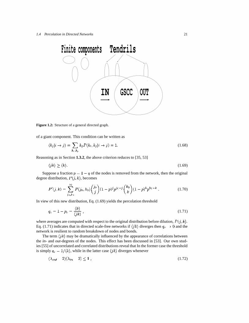
of the WWW in [54, 8]. In general, a directed graph consists of a giant weakly connectedcomponent (GWCC) and several finite components. In the GWCC every site is reachablefrom every other, provided that the links are treated as bi-directional. The GWCC is furtherdivided into a giant strongly connected component (GSCC), consisting of all sites reachablefrom each other following directed links. All the sites reachable from the GSCC are referredto as the giant OUT component, and the sites from which the GSCC is reachable are referredto as the giant IN component. The GSCC is the intersection of the IN and OUT components.Sites in the GWCC, but not in the IN and OUT components, constitute the “tendrils” (see Fig.1.2.).

Here we repeat the analysis of Section 1.3 for the case of directed networks. We limitourselves mostly to final results and conclusions. A detailed derivation can be found in [55].

1.4.1 Threshold

The condition for the existence of a giant component in a directed random network of arbitrarydegree distribution can be deduced in a manner similar to [14]. If a site is reached following alink pointing to it, then it must have at least one outgoing link, on average, in order to be part

1.4 Percolation in Directed Networks 21

GSCC OUTIN

TendrilsFinite components

Figure 1.2: Structure of a general directed graph.

of a giant component. This condition can be written as

� �� $�� $�� ? (1.68)

Reasoning as in Section 1.3.2, the above criterion reduces to [35, 53]

�� ? (1.69)

Suppose a fraction � � � � of the nodes is removed from the network, then the originaldegree distribution, �� , becomes

� � ��

�� ? (1.70)

In view of this new distribution, Eq. (1.69) yields the percolation threshold

� � � � � � � � �� (1.71)

where averages are computed with respect to the original distribution before dilution, �� .Eq. (1.71) indicates that in directed scale-free networks if �� diverges then � � $ � and thenetwork is resilient to random breakdown of nodes and bonds.

The term �� may be dramatically influenced by the appearance of correlations betweenthe in- and out-degrees of the nodes. This effect has been discussed in [53]. Our own stud-ies [55] of uncorrelated and correlated distributions reveal that In the former case the thresholdis simply � � � �

;� �� , while in the latter case �� diverges whenever

�� !�� (1.72)


2 3 4 5 6λ

out

2

3

4

5

6

λin

Resilient

Anomalous

Mean field

exponents

exponents

Figure 1.3: Phase diagram of the different regimes for the IN component of scale-free correlated di-rected networks. The boundary between Resilient and Anomalous exponents is derived from Eq. (1.72)while that between Anomalous exponents and Mean field exponents is given in table 1.1 for �� .For the diagram of the OUT component �� and �� change roles

causing the percolation threshold to vanish. The various regimes resulting from this observa-tion are summarized in Fig. 1.3.

Percolation of the GWCC can be seen to be similar to percolation in the non-directed graphcreated from the directed graph by ignoring the directionality of the links. The threshold isobtained from the criterion (cf Eq. (1.27))

�� ? (1.73)

Here the connectivity distribution is the convolution of the in and out distributions,

� � � ��

�� ? (1.74)

Whether the distribution is correlated or not, �� is always dominated by the slower decay-exponent, therefore percolation of the GWCC is the same as in non-directed scale-free net-works, with �� = � � �� !

�. Note that the percolation threshold of the GWCC may

differ from that of the GSCC and the IN and OUT components [53].

1.4.2 Critical exponents

Percolation of the GSCC and IN and OUT components may be analyzed with the formalism ofgenerating functions [44, 39, 35, 53] (see, also, the Chapter by Newman in this book). We have

1.5 Efficient Immunization Strategies 23

uncorrelated correlatedGWCC

= � � �� ! � � � � � � = � � �� ! � � �

�IN � � ! � � � � ! � ��

OUT � � � � � �

� � �� GSCC

= � � �� ! � � � � � � = � � �� ! � � ��

�

Table 1.1: Values of � � for the different network components for both correlated and uncorrelated cases.

computed the critical exponents � and � , following the approach of Section 1.3.5. The resultsare the same as for the non-directed case, Eqs. (1.49) and (1.54), but where � is replaced by aneffective � � whose value differs for uncorrelated and correlated distributions. The value of � �for the various components in both the uncorrelated and correlated scenario are summarizedin table 1.1. Our findings [55] indicate that even the tiniest amount of correlation results inbehavior typical to the correlated case. We may therefore conclude that in practical situationsonly the correlated case counts, for it is expected, to some extent, in most naturally occurringdirected networks.

1.5 Efficient Immunization Strategies

It is well established that random immunization fails to prevent epidemics of diseases thatspread upon contact between infected individuals. On the other hand, targeted immunizationrequires global knowledge of the topology of the social network in question, rendering itimpractical. We propose an effective strategy, based on the immunization of a small fractionof random acquaintances of randomly selected individuals, that prevents epidemics withoutrequiring global knowledge of the network [56].

Social networks are known to possess a broad distribution of the number of links (con-tacts)

�, emanating from a node (an individual) [57, 58, 59, 10]. 3 Studies of percolation

on broad distribution networks show that a large fraction� �

of the nodes need to be removed(immunized) before the integrity of the network is compromised. This is particularly true forscale-free networks with �� — the case of most known networks [6, 9, 13] — wherethe percolation threshold

�� $ � , and the network remains connected (contagious) even afterimmunization of most of its nodes [60, 61, 62, 63, 45, 14, 39]. In other words, with a randomimmunization strategy most of the population needs to be immunized before an epidemic isarrested (see Fig. 1.4).

When the most highly connected nodes are targeted first, removal of just a small fractionof the nodes results in the network’s disintegration [39, 41]. This has led to the suggestion oftargeted immunization of the HUBs (the most highly connected nodes in the network) [64, 65].The main shortcoming of this approach is that it requires a complete, or at least fairly goodknowledge of the connectivity of each node in the network. Such global information oftenproves hard to gather, and may not even be well-defined (as in social networks, where thenumber of social relations depends on subjective judging). Here we propose an effective

3Often this is the scale-free distribution �� . Our results apply, however, to broad distributions ingeneral.


immunization strategy that works at low immunization rates�

, and obviates the need forglobal information.

1.5.1 Acquaintance immunization

In our approach, we choose a random fraction of the population (of size � ) and ask eachindividual to point at an acquaintance with whom they are in contact. The acquaintances,rather than the individuals themselves, are the ones immunized. The fraction

� �needed to be

immunized in order to stop the epidemic can be computed analytically.In each immunization event the probability that a node with

�contacts is selected is� ��

;��)� �� . Let � � � � � be the number of individuals in chemical shell

who are sus-

ceptible (not immunized). In the next chemical shell, � � , each of those sites connects to� � � neighbors (excluding the one connecting to shell �>� ). To find out � �� , we mul-

tiply the number of links going out of theth layer by the probability of reaching a site of

connectivity� � by following a link from a susceptible site, � � � � �� , and the probability

that this site is also susceptible, � � �� . This gives

� �� *� � � � � � �� ? (1.75)

From Bayes’ rule,

� � � � �� ? (1.76)

� � � � �� ; � �� is independent of�

. � � � � �� 5 � � 2 � � � � 5 � � 2 � � � �� , where theaverage is taken with respect to � �� as defined before. � � � � �� ; ��C� � , since noknowledge exists on its neighbors. Using all these relations one obtains:

� � � � �� 5 � � 2 � �� 5 � �2 � � ? (1.77)

The above results, along with (1.75) yield

� �� 5 � � 2 � � � � � � � � � � � � � � 5 � �2 �� (1.78)

where � � �� ; �� . This leads to the stable distribution of connectivity in a chemical

layer: � � � � � �� 5 � �2 �

, for some�. Putting this back into (1.78) results in:

� �� *� �� 5 � � � 2 � ? (1.79)

Therefore, if the sum in (1.79) is larger than � the population is above the percolation thresholdand the epidemics would propagate, while it would be arrested if the sum is smaller than � .Thus,

� � � � � � � � � �� 5 �

� �� 2 � � � � (1.80)

1.6 Summary and Outlook 25

2 2.5 3 3.5λ

0

0.2

0.4

0.6

0.8

1

fc

Figure 1.4: Critical probability, �� , as a function of � , for the random immunization (top), acquain-tance immunization (middle), double acquaintance immunization (lower middle) and attack (bottom)strategies. Curves represent analytical results (approximate for double acquaintace), while data pointsrepresent simulation data, for a population � �� .

is the condition for criticality. The desired immunization fraction then follows:� � � � � ��

�� ? (1.81)

A related immunization strategy calls for the immunization of acquaintances referred toby at least � individuals. (Above, we specialized to � � � .) The threshold is lower the larger� is, and may justify, under certain circumstances, this somewhat more involved protocol.

In Fig. 1.4, we show the immunization threshold� �

needed to stop an epidemic in net-works with � �� ? � (this covers all known cases). Plotted are curves for the (inefficient)random strategy, and the strategy advanced here, for the cases of � � � and � . Note the dra-matic decrease of

� �with the suggested strategy. Improvements can be achieved for any broad

distribution.Various immunization strategies have been proposed earlier, mainly for the case of an

already spread disease and are based on tracing the chain of infection towards the super-spreaders of the disease [66]. Our approach can be used even before the epidemic startsspreading, and therefore does not require any knowledge of the chain of infection.

1.6 Summary and Outlook

The main goal of this chapter has been to study the effect of the special nature of scale-freedistribution on the properties of random network models. Some general methods have beenpresented for the study of generalized random networks. Those include methods for the studyof the layer structure of the graph, the percolation threshold and the critical exponents.


The special properties of scale-free networks, in conjunction with the general methodpresented for the study of scale-free and other networks, might prove useful for applicationssuch as the design of more robust networks [40], the improvement of routing [67] and searchalgorithms [68], and the predicting and arresting of computer and human viruses [45, 65].

Acknowledgments

We would like to thank Keren Erez, Nehemia Schwartz, Alejandro Rozenfeld and Albert-Lazslo Barabasi for their collaboration, help and insights on many of the topics covered in thischapter. DbA thanks the support of the National Science Foundation (USA).

References

[1] P. Erdos and A. Renyi, On random graphs. Publicationes Mathematicae 6, 290–297(1959).

[2] P. Erdos and A. and Renyi, On the evolution of random graphs. Publications of theMathematical Institute of the Hungarian Academy of Sciences 5, 17–61 (1960).

[3] P. Erdos, and A. Renyi, On the strength of connectedness of a random graph. ActaMathematica Scientia Hungary 12, 261–267 (1961).

[4] B. Bollobas, Random Graphs. Academic Press, New York (1985).

[5] A.-L. Barabasi and R. Albert, Emergence of scaling in random networks. Science 286,509–512 (1999).

[6] M. Faloutsos, P. Faloutsos and C. Faloutsos, On power-law relationships of the internettopology. Computer Communications Review 29, 251–262 (1999).

[7] A.-L. Barabasi, R. Albert and H. Jeong, Scale-free characteristics of random networks:the topology of the World-Wide Web Physica A, 281, 69–77 (2000).

[8] A. Broder, R. Kumar, F. Maghoul, P. Raghavan, S. Rajagopalan, R. Stata, A. Tomkins J.Wiener, Graph structure in the web. Computer Networks 33, 309–320 (2000).

[9] H. Ebel, L.-I. Mielsch and S. Bornholdt, Scale-free topology of e-mail networks.Preprint cond-mat/0201476 (2002).

[10] S. Redner, How popular is your paper? An empirical study of the citation distribution.Eur. Phys. J. B 4, 131–134 (1998).

[11] H. Jeong, B. Tombor, R. Albert, Z. N. Oltvai and A.-L. Barabasi, The large-scale orga-nization of metabolic networks Nature, 407, 651, (2000).

[12] H. Jeong, S. P. Mason, A.-L. Barabasi, and Z. N. Oltvai, Lethality and centrality inprotein networks. Nature 411, 41–42 (2001).

[13] X. Guardiola, R. Guimera, A. Arenas, A. Diaz-Guilera, D. Streib and L. A. N. Amaral,Macro- and micro-structure of trust networks. Preprint cond-mat/0206240 (2002).

References 27

[14] R. Cohen, K. Erez, D. ben-Avraham and S. Havlin, Resilience of the Internet to RandomBreakdown. Phys. Rev. Lett. 85, 4626–4628 (2000).

[15] S. N. Dorogovtsev and J. F. F. Mendes, Natural Scale of Scale-free Networks. Phys. Rev.E 63, 62101 (2001).

[16] G. Bianconi and A.-L. Barabasi, Bose-Einstein condensation in complex networks. Phys.Rev. Lett. 86, 5632–5635 (2001).

[17] P. L. Krapivsky, S. Redner and F. Leyvraz, Connectivity of Growing Random Networks.Phys. Rev. Lett. 85, 4629–4632 (2000).

[18] M. Molloy and B. Reed, A critical point for random graphs with a given degree sequence.Random Structures and Algorithms 6, 161–179 (1995).

[19] M. Molloy and B. Reed, The size of the giant component of a random graph with a givendegree sequence. Combin. Probab. Comput. 7, 295–305 (1998).

[20] W. Aiello, F. Chung and L. Lu, A random graph model for massive graphs. In Pro-ceedings of the 32nd Annual ACM Symposium on Theory of Computing, pp. 171–180.Association of Computing Machinery, New York (2000).

[21] A. Bunde and S. Havlin (eds.), Fractals in Science. Springer, New York (1994).[22] A. Bunde and S. Havlin (eds.), Fractals and Disordered System. Springer, New York

(1996).[23] P. Levy, Calcul des Probabilities. Gauthier Villars, Paris (1925).[24] M. F. Shlesinger and J. Klafter, Accelerated Diffusion in Josephson Junctions and Re-

lated Chaotic Systems. Phys. Rev. Lett. 54, 2551 (1985).[25] J. Klafter, M. F. Shlesinger and G. Zumofen, Beyond Brownian motion. Phys. Today 49,

33 (1996).[26] G. M. Viswanathan, S. V. Buldyrev, S. Havlin, M. G. E. da Luz, E. P. Raposo and H. E.

Stanley, Optimizing the success of random searches. Nature 401, 911 (1999).[27] J. M. Kleinberg, Navigation in a Small World. Nature 406, 845 (2000).[28] R. Albert and A.-L. Barabasi, Statistical mechanics of complex networks. Rev. Mod.

Phys. 74, 47–97 (2002).[29] S. N. Dorogovtsev and J. F. F. Mendes, Evolution of networks. Adv. in Phys. 51, 1079–

1187 (2002).[30] D. ben-Avraham and S. Havlin, Diffusion and Reactions in Fractals and Disordered

Systems. Cambridge University Press, Cambridge (2000).[31] D. J. Watts and S. H. Strogatz, Collective dynamics of ‘small-world’ networks. Nature

393, 440–442 (1998).[32] D. J. Watts, Small Worlds. Princton University Press, Princeton (1999).[33] A. F. Rozenfeld, R. Cohen, D. ben-Avraham and S. Havlin, Scale-free Networks on

Lattices. Preprint cond-mat/0205613 (2002).[34] R. Cohen and S. Havlin, Ultra Small World in Scale-Free Networks. Preprint cond-

mat/0205476 (2002).[35] M. E. J. Newman, S. H. Strogatz and D. J. Watts, Random graphs with arbitrary degree

distributions and their applications. Phys. Rev. E 64, 026118, (2001).[36] B. Bollobas and O. Riordan, The diameter of a scale-free random graph process Preprint

(2001).


[37] G. Szabo, M. Alava and J. Kertesz, Shortest paths and load scaling in scale-free treesPreprint cond-mat/0203278 (2002).

[38] D. Stauffer and A. Aharony, Introduction to Percolation Theory. Taylor and Francis,London, 2nd edition (1992).

[39] D. S. Callaway, M. E. J. Newman, S. H. Strogatz and D. J. Watts, Network robustnessand fragility: Percolation on random graphs. Phys. Rev. Lett. 85, 5468–5471 (2000).

[40] R. Albert, H. Jeong and A.-L. Barabasi, Attack and error tolerance of complex networks.Nature 406, 378–382 (2000).

[41] R. Cohen, K. Erez, D. ben-Avraham and S. Havlin, Breakdown of the Internet underIntentional Attack. Phys. Rev. Lett. 86, 3682–3685 (2001).

[42] R. Cohen, D. ben-Avraham and S. Havlin, Percolation Critical Exponents in Scale-FreeNetworks. Cond-mat/0202259 (2002); Phys. Rev. E (in press, 2002).

[43] G. H. Weiss, Aspects and Applications of the Random Walk. North-Holland, Amsterdam,(1994).

[44] H. S. Wilf, Generatingfunctionology 2nd ed. Academic Press, London, (1994).[45] R. Pastor-Satorras and A. Vespignani. Epidemic spreading in scale-free networks. Phys.

Rev. Lett. 86, 3200–3203 (2001).[46] R. Pastor-Satorras and A. Vespignani. Epidemic dynamics and endemic states in com-

plex networks. Phys. Rev. E 63, 066117 (2001).[47] Y. Moreno, R. Pastor-Satorras and A. Vespignani, Epidemic outbreaks in complex het-

erogeneous networks. Eur. Phys. J. B 26, 521–529 (2002).[48] D. S. Callaway, J. E. Hopcroft, J. M. Kleinberg, M. E. J. Newman and S. H. Strogatz,

Are randomly grown graphs really random? Phys. Rev. E, 64, 041902 (2001).[49] S. N. Dorogovtsev and J. F. F. Mendes, Anomalous percolating properties of growing

networks Phys. Rev. E 64, 066110 (2001).[50] Z. Burda, J. D. Correia and A. Krzywicki, Statistical ensemble of scale-free random

graphs. Phys. Rev. E 64, 046118 (2001).[51] F. Chung, and L. Y. Lu, The diameter of sparse random graphs. Adv. Appl. Math., 26,

257, (2001).[52] S. H. Strogatz, Exploring complex networks. Nature 410, 268–276 (2001) .[53] S. N. Dorogovtsev, J. F. F. Mendes and A. N. Samukhin, Giant strongly connected

component of directed networks. Phys. Rev. E 64, 025101 (2001).[54] R. Albert, H. Jeong and A.-L. Barabasi, Diameter of the world-wide web. Nature 401,

130–131 (1999).[55] N. Schwartz, R. Cohen, D. ben-Avraham, A.-L. Barabasi and S. Havlin, Percolation in

Directed Scale-Free Networks. Phys. Rev. E 66, in press (2002).[56] R. Cohen, D. ben-Avraham and S. Havlin, Efficient immunization of populations and

computers. Preprint cond-mat/0207387 (2002).[57] F. Liljeros, C. R. Edling, L. A. N. Amaral, H. E. Stanley and Y. Aberg, The web of

human sexual contacts. Nature 411, 907–908 (2001).[58] M. E. J. Newman, The structure of scientific collaboration networks. Proc. Natl. Acad.

Sci. USA 98, 404–409 (2001).

References 29

[59] R. V. Sole and J. M. Montoya, Complexity and fragility in ecological networks Proc.Roy. Soc. Lond. B Bio. 268, 2039–2045, (2001).

[60] R. M. Anderson, and R. M. May, Infectious Diseases of Humans. Oxford UniversityPress, Oxford (1991).

[61] A. L. Lloyd and R. M. May, How viruses spread among computers and people. Science292, 1316–1317 (2001).

[62] C. P. Warren, L. M. Sander, I. Sokolov, C. Simon and J. Koopman, Percolation ondisordered networks as a model for epidemics. Math. Biosci., in press (2002).

[63] M. E. J. Newman, Exact solutions of epidemic models on networks. Preprint cond-mat/0201433 (2002).

[64] Z. Dezso and A.-L. Barabasi, Halting viruses in scale-free networks, Preprint cond-mat/0107420 (2001).

[65] R. Pastor-Satorras and A. Vespignani, Immunization of complex networks. Phys. Rev. E65, 036104 (2001).

[66] W. H. Wethcote and J. A. Yorke, Gonorrhea transmission dynamics and control. Lecturenotes in Biomathematics 56, (Springer-Verlag, 1984).

[67] K.-I. Goh, B. Kahng, D. Kim, Universal Behavior of Load Distribution in Scale-freeNetworks. Phys. Rev. Lett. 87, 278701 (2001).

[68] L. A. Adamic, R. M. Lukose, A. R. Puniyani, B. A. Huberman, Search in Power-LawNetworks. Phys. Rev. E 64, 046135 (2001).

structural properties of scale-free networks

Documents