1

Steam Turbine Optimisation for

Solar Thermal Power Plant Operation

James D. Spelling

Licentiate Thesis

KTH Royal Institute of Technology

School of Industrial Engineering and Management

Division of Heat and Power Technology

Stockholm, Sweden

2

Printed in Sweden Universitetsservice US-AB Stockholm 2011

TRITA KRV Report 11/03

ISSN 1100-7990 ISRN KTH/KRV/11/03-SE ISBN 978-91-7415-991-2

© James Spelling, 2011

3

Abstract

The provision of a sustainable energy supply is one of the most important issues facing humanity at the current time, given the strong dependence of social and economic prosperity on the availability of affordable energy and the growing environmental concerns about its production. Solar thermal power has established itself as a viable source of renewable power, capable of generating electricity at some of the most economically attractive rates.

Solar thermal power plants are based largely on conventional Rankine-cycle power generation equipment, reducing the technological risk involved in the initial investment. Nevertheless, due to the variable nature of the solar supply, this equipment is subjected to a greater range of operating conditions than would be the case in conventional systems.

The necessity of maintaining the operational life of the steam-turbines places limits on the speed at which they can be started once the solar supply becomes available. However, in order to harvest as much as possible of the Sun’s energy, the turbines should be started as quickly as is possible. The limiting factor in start-up speed being the temperature of the metal within the turbines before start-up, methods have been studied to keep the turbines as warm as possible during idle-periods.

A detailed model of the steam-turbines in a solar thermal power plant has been elaborated and validated against experimental data from an existing power plant. A dynamic system model of the remainder of the plant has also been developed in order to provide input to the steam-turbine model.

Three modifications that could potentially maintain the internal temperature of the steam-turbines have been analysed: installation of additional insulation, increasing the temperature of the gland steam and use of external heating blankets. A combination of heat blankets and gland steam temperature increase was shown to be the most effective, with increases in electricity production of up to 3% predicted on an annual basis through increased availability of the solar power plant.

Keywords: solar thermal power, steam-turbine, start-up, cool-down, dispatchability increase

4

5

Sammanfattning

Hållbar energiförsörjning är för närvarande en av de viktigaste frågorna för mänskligheten. Socialt och ekonomiskt välstånd är starkt kopplat till rimliga energipriser och hållbar energiproduktion. Koncentrerad solenergi är nu etablerat som en tillförlitlig källa av förnybar energi och är ett ekonomiskt attraktivt alternativ. Koncentrerade solenergikraftverk bygger till stor del på konventionell Rankine-cykel elgeneratorer, vilka minskar de tekniskt relaterade riskerna i den initiala investeringen. På grund av solstrålningens skiftande karaktär utsätts denna utrustning för mer varierade driftsförhållanden, jämfört med konventionella system.

Behovet av att bibehålla den operativa livslängden på ångturbiner sätter gränser för uppstartshastigheten när solstrålningen blir tillgänglig. För att utnyttja så mycket som möjligt av solens energi bör ångturbinen startas så snabbt som möjligt. Eftersom temperaturen i metalldelar hos turbinerna är den begränsande faktorn, metoder har studerats för att hålla turbinerna så varma som möjligt under tomgångsperioder.

En detaljerad modell av ångturbiner i ett solenergikraftverk har utvecklats och validerats mot experimentella data från ett befintligt kraftverk. En dynamisk systemmodell av de övriga delarna av anläggningen har också utvecklats för att ge input till ångturbinsmodellen.

Tre modifieringar som eventuellt kan upprätthålla den inre temperaturen i ångturbiner har analyserats: montering av ytterligare isolering, ökning av temperaturen hos glänsångan och användning av elvärmefiltar. En kombination av värmefiltar och en temperaturökning av glänsångan visade sig vara det mest effektiva. Åtgärderna resulterade i en ökad elproduktion på upp till 3%, beräknat på årsbasis genom ökad tillgänglighet hos kraftverket.

Nyckelord: koncentrerad solenergi, ångturbin, uppstart, nedkylning, ökad flexibilitet

6

7

Preface

This thesis has been performed at the Division of Heat and Power Technology within KTH’s Department of Energy Technology, part of the School of Industrial Engineering and Management. Research at the Division of Heat and Power Technology is focused on all aspects of climate neutral and socially acceptable energy sources that could be deployed to meet future energy needs.

P u b l i c a t i o n s

This licentiate thesis is based upon three publications:

1. T. Strand, J. Spelling, B. Laumert, T. Fransson, “On the Significance of Concentrated Solar Power R&D in Sweden”, Proceedings of the World Renewable Energy Congress, Linköping, May 2011

2. J. Spelling, M. Jöcker, A. Martin, “Thermal Modelling of a Solar Steam-Turbine with a focus on Start-Up Time Reduction”, GT2011-45686, Proceedings of the ASME Turbo Expo, Vancouver, June 2011

3. J. Spelling, M. Jöcker, A. Martin, “Annual Performance Improvement for Solar Steam-Turbines through the use of Temperature-Maintaining Modifications”, Journal of Solar Energy (manuscript under review)

The contribution of the author of this thesis to the different publications is as follows:

Paper 1: The idea for the paper was initiated by Prof. Strand. The author was responsible for the preparation of the majority of the text. Additionally, all novel results and analyses presented are based on the work of the author.

Paper 2: Main author; performed all simulations and analyses. The on-site measurement data was obtained by Dr. Jöcker, who also provided the technical information on the turbine units under study.

Paper 3: Main author; performed all simulations and analyses.

8

A c k n o w l e d g e m e n t s

Firstly, I would like to thank my supervisor, Prof. Andrew Martin, for his advice and guidance throughout the writing of this Licentiate thesis, as well as to our department head: Prof. Torsten Fransson, for giving me the opportunity to come to KTH and study in the beautiful city that is Stockholm.

I would also like to thank Dr. Markus Jöcker of Siemens Industrial Turbomachinery for his advice, suggestions and technical insights into the steam-turbines under study. Your expertise has been invaluable.

Thanks also to Dr. Björn Laumert for your support, advice and especially the clear-cut reviewing of my papers: they are greatly improved as a result your comments!

This research has been funded by the Swedish Energy Agency, Siemens Industrial Turbomachinery, Volvo Aero Corporation and the Royal Institute of Technology through the Swedish research program: TURBO POWER, the support of which is gratefully acknowledged. Thanks are also given to the Industrial Energy Systems Laboratory of the Swiss Federal Institute of Technology, Lausanne for the use of their multi-objective optimisation algorithm: QMOO.

To my dear colleagues and friends at the Department of Energy Technology: Tomas, Johannes, Mafe, Florian, Justin, Ranjan and Monika, thanks for the coffee, discussions and PhD pubs, they made this thesis fun to write and kept me going through the long nights of the Nordic winter.

9

N o m e n c l a t u r e

C h a r a c t e r s

A Surface Area [m2] c Specific Heat Capacity [J/kgK] C Heat Capacity Rate [W/K] Cr Ratio of Heat Capacity Rates [ - ] CR Concentration Ratio [ - ] d Diameter [m] DNI Direct Normal Irradiation [W/m2] e Thickness [m] E Mechanical/Electrical Power [W] f Heat Transfer Correction Factor [ - ] Solar Field Efficiency Factor [ - ] g Acceleration due to Gravity [m/s2] G Mass Flux [kg/m2s] h Specific Enthalpy [J/kg] Tank Filling Height [m] Time [hrs] I Solar Radiation Flux [W/m2] k Material Thermal Conductivity [W/mK] ks Surface Roughness [m] K Thermal Conductivity Matrix [W/mK] l Length [m] L Earth-Sun Distance [m] LEC Levelised Cost of Electricity [cts/kWhe] M Mass Flow Rate [kg/s] Correction Magnitude [ - ] n Gregorian Calendar Day [ - ] Current Timestep Number [ - ] n Surface Normal Vector [m] N Rotational Speed [rpm] Number of Daylight Hours [hrs] Number of Timesteps [ - ] NTU Number of Transfer Units [ - ] Nu Nusselt Number [ - ] r Radial Position [m] R Heat Transfer Resistance [m2K/W ] Re Reynolds Number [ - ] Rs Radius of the Sun [m] P Pressure [Pa] Perimeter Length [m] Pr Prandtl Number [ - ] q Heat Flux [W/m2] Q Thermal Power [W]

10

t Time [s] T Temperature [K] u Specific Internal Energy [J/kg] Flow Speed [m/s] U Global Heat Transfer Coefficient [W/m2K] V Volume [m3] w Width [m] Y Stodola Ellipse Constant [m2s2K] z Axial Position [m]

S y m b o l s

α Material Absorptivity [ - ] Heat Transfer Coefficient [W/m2K] β Coefficient of Thermal Expansion [K-1] ΔTmin Minimum Approach Temperature [K] γs Solar Azimuth Angle [rad] δ Declination Angle [rad] δs Angular Size of Solar Disk [rad] ε Material Emissivity [ - ] Volumetric Void Fraction [ - ] Heat Transfer Effectiveness [ - ] η Efficiency [ - ] θ Incidence Angle [rad] θz Solar Elevation Angle [rad] ν Kinematic Viscosity [m2/s] П Pressure Ratio [ - ] ρ Material Density [kg/m3] Mirror Reflectivity [ - ] ς Steam Extraction Fraction [ - ] σ Stefan Boltzmann Constant [W/m2K4] τ Material Transmissivity [ - ] φ Latitude [°N] Tangential Position [rad] Finned Surface Multiplication Factor [ - ] Ф Mass Flow Coefficient [ms K½] Ψ Longitude [°W] ω Solar Hour Angle [rad]

S u b s c r i p t s

a Atmospheric e External Axial eff Effective adb Adiabatic ext Extraction Point b At Bulk Conditions f Fluid Phase cond Conduction Fin

11

gst Gland Steam p Pump h Homogeneous At Constant Pressure HP High Pressure r Radial HPT High Pressure Turbine s Solid Phase i Element Number Isentropic Internal st Steam Spatial Index tub Tube Connection Number v Volumetric LP Low Pressure • Temporal Derivative LPT Low Pressure Turbine - Leaving System m Metal + Entering System n Temporal Index o Origin

12

13

Table of Contents

ABSTRACT ................................................................................................... 3

PREFACE ...................................................................................................... 7

PUBLICATIONS ............................................................................................. 7 ACKNOWLEDGEMENTS ................................................................................ 8 NOMENCLATURE.......................................................................................... 9

TABLE OF CONTENTS ............................................................................ 13

1 INTRODUCTION .............................................................................. 15

1.1 CONTEXT ...................................................................................... 15 1.2 OBJECTIVES .................................................................................. 17 1.3 METHODOLOGY ............................................................................ 17

1.3.1 Dynamic Simulation Model ..................................................... 17 1.3.2 Steam Turbine Modification .................................................... 18

1.4 THESIS STRUCTURE ...................................................................... 18

2 FUNDAMENTAL NOTIONS ........................................................... 21

2.1 SOLAR ENERGY RESOURCES ......................................................... 21 2.1.1 Renewable Energy Sources...................................................... 21 2.1.2 Solar Radiation and Energy Supply......................................... 22

2.2 CONCENTRATED SOLAR POWER ................................................... 24 2.2.1 Solar Concentration ................................................................ 25 2.2.2 Linear Concentration Devices ................................................. 26 2.2.3 Point Focus Concentration Devices ........................................ 27

2.3 SOLAR THERMAL POWER PLANTS (PAPER 1) ................................ 28 2.4 ANDASOL 1 SOLAR POWER PLANT ............................................... 30

3 TRANSIENT MODELLING OF SOLAR STEAM TURBINES ... 33

3.1 FINITE VOLUME MODEL ............................................................... 33 3.1.1 Heat Conduction Equation ...................................................... 33 3.1.2 Geometry Simplification .......................................................... 34 3.1.3 Finite Volume Techniques ....................................................... 37 3.1.4 Boundary Conditions ............................................................... 38

3.2 STEAM EXPANSION MODEL .......................................................... 39 3.2.1 Stodola Expansion Model ........................................................ 40 3.2.2 Non-Adiabatic Expansion Model ............................................. 41 3.2.3 Heat Transfer Calculation ....................................................... 42

3.3 GLAND STEAM NETWORK MODEL ................................................ 43 3.4 THE LOW-PRESSURE TURBINE ...................................................... 44

3.4.1 Geometry Simplification/Meshing ........................................... 44 3.4.2 Boundary Conditions ............................................................... 45

3.5 THE HIGH-PRESSURE TURBINE ..................................................... 46 3.5.1 Geometry Simplification/Meshing ........................................... 46 3.5.2 Boundary Conditions ............................................................... 48

14

3.6 MODEL VALIDATION .................................................................... 48 3.6.1 Validation Data ....................................................................... 48 3.6.2 Initial Validation Results ......................................................... 49 3.6.3 Model Parameter Correction .................................................. 51 3.6.4 Final Validation Results .......................................................... 53 3.6.5 Sensitivity Analysis .................................................................. 54

4 DYNAMIC MODELS OF POWER PLANT COMPONENTS ...... 57

4.1 SOLAR GEOMETRY ....................................................................... 57 4.2 PARABOLIC TROUGH COLLECTORS............................................... 59

4.2.1 Parabolic Mirror Concentrator ............................................... 59 4.2.2 Vacuum Tube Receivers ........................................................... 62

4.3 TWO-TANK MOLTEN SALT STORAGE ........................................... 67 4.4 REHEAT STEAM GENERATOR ........................................................ 70

4.4.1 The Effectiveness-NTU Design Method ................................... 71 4.4.2 Off-Design Performance .......................................................... 73 4.4.3 Pinch Analysis Techniques ...................................................... 74

4.5 FEEDWATER PUMP ........................................................................ 76

5 POWER PLANT PERFORMANCE IMPROVEMENT ................ 79

5.1 STEAM TURBINE MODIFICATIONS................................................. 80 5.1.1 Installation of Additional Insulation ........................................ 81 5.1.2 Installation of Heat Blankets ................................................... 81 5.1.3 Increasing Gland Steam Temperature ..................................... 82

5.2 DAILY IMPROVEMENT (PAPER 2) .................................................. 83 5.2.1 Key Results .............................................................................. 83

5.3 ANNUAL IMPROVEMENT (PAPER 3) .............................................. 86 5.3.1 Key Results .............................................................................. 87

6 CONCLUSIONS ................................................................................. 91

6.1 OUTLOOK ..................................................................................... 92

REFERENCES ............................................................................................ 93

APPENDIX: INSULATION DATA ........................................................... 97

APPENDIX: PAPERS................................................................................. 99

15

1 Introduction

1 . 1 C o n t e x t

Amidst a backdrop of rapidly increasing world-wide electricity demand, the development of new renewable energy technologies is of primary importance in the effort to reduce emissions of carbon dioxide and other greenhouse gases. In addition, rapid increases in the price of oils coupled with worries about the stability and security of the extraction of fossil fuels, has led to a renewed interest in the development of local energy resources, thereby reducing dependence on foreign supplies [11].

Solar power generation shows great potential [33] for supplying the electricity needs of numerous countries in the Sun-belt regions of the world. In these regions, the absence of significant biomass, hydrological or geothermal reserves makes solar power the most promising solution for meeting that most fundamental of demands: energy. Amidst the different options available for harnessing the Sun’s power, solar thermal technologies have been shown capable of producing electricity at the most economically viable rates [22]. This has led to a recent renewal in the development of such systems [25], most notably with the construction of the Andasol parabolic trough power plants in Spain, and the Nevada Solar One power plant in the United States.

All existing commercial solar thermal power plants are based on the use of Rankine, or steam-turbine, cycles. Steam-turbine operation in solar thermal power plants is very different from that occurring in traditional base-load power plants. As a result of the variable nature of the solar supply and the daily operating cycle of solar power plants, the number of turbine starts per year for solar steam-turbines is an order of magnitude higher than for base-load turbines.

The current generation of steam-turbine equipment used in solar thermal power plants is characterised by a high thermal flexibility due, for example, to the barrel casing design of the high pressure turbine and the slim design of the low pressure turbine ([15], [20]). Still, operational requirements demand full utilisation of this flexibility: turbomachinery operated in solar thermal power plants are subjected to a much higher variability in working conditions, with multiple starts possible during a 24h period. This requires turbine component optimisation to avoid excessive thermal stresses and low cycle fatigue in the casing and rotor of the turbine during start-up, shut down and load variations [13]. Due to the uncontrollable nature of the solar supply, it is also desirable that the turbine be able to start as quickly as possible, in order for the plant to be

16

able to harvest as much as possible of the Sun’s energy once it becomes available.

In order to avoid excessive thermal stress within the turbines during start-up, and thus preserve the lifetime of the units, the manufacturer specifies start-up curves which limit the speed at which the turbines can reach full load, based on the lowest metal temperature measured before start-up begins, as shown in Figure 1.1.

Figure 1.1. Turbine start-up time as a function of the minimum temperature measured in the unit before start-up.

If the turbine components cool-down below a certain limit, the start-up time of the unit is drastically increased, limiting the dispatchability of the solar power plant (which is a measure of its ability to respond to changes in electrical demand).

For each temperature range shown in Figure 1.1, a start-up curve is given by the manufacturer, which specifies the operating conditions to be set during the start-up period until the turbine reaches full load. Cold starts require slow increases in load to limit the thermal stresses, whereas warm and hot starts allow full load to be reached much more quickly. This is shown for three example start-up curves in Figure 1.2.

Figure 1.2. Cold, warm and hot turbine start-up curves.

17

Previous studies ([2], [30]) have focused on the reduction of rapid temperature and pressure transients in the solar steam supply during operation in order to avoid excessive thermal stresses and the corresponding lifetime reduction. Other works have studied means of changing operating procedures to achieve faster start-up times [9]. Prior simulation of a solar steam-turbine [3] has analysed performance during solar transients, though only a simplified model was used for evaluation of the metal temperatures and thermal gradients within the turbine units

All these studies overlook a potential area for operational improvement, namely that the limiting factor in achieving faster starts without harming the turbine is the cooling down of the metal during idle periods. As such, if the steam-turbine can be kept warm during idle periods, the duration of the next start-up can be reduced without impacting negatively on the lifetime.

1 . 2 O b j e c t i v e s

The focus of this work is placed on finding means of increasing the dispatchability of the steam-turbines operating in solar thermal power plants without exceeding the stress limits placed by the manufacturers, thus preserving (or even improving) the lifetime of the steam-turbine units.

The approach taken in this study is to maintain the turbine components at a higher temperature during idle, or cool-down, periods, thus allowing the use of the faster warm and hot start-ups. This will not only allow the turbine to start faster once the Sun's energy becomes available; in the case of a switch from a cold to a warm start-up, a significant increase in diurnal output of the power plant can be expected.

1 . 3 M e t h o d o l o g y

1 . 3 . 1 D y n a m i c S i m u l a t i o n M o d e l

A detailed model of the transient heat conduction within both the high-pressure and low-pressure solar steam-turbines has been developed; combining a finite-volume heat conduction model with a Stodola-based model [6] for the steam expansion, allowing prediction of the dynamic behaviour of the turbine during off-design operation. This model has been validated using experimental data from an existing solar steam-turbine at the Andasol 1 power plant in Spain.

In addition to this detailed steam-turbine model, dynamic system models have been developed for the different components of a solar steam-turbine power plant as part of KTH’s in-house SOLARDYN modelling

18

tool [27]. Coupled with the detailed solar steam-turbine model, this will allow analysis of the performance of the complete power plant. To simplify the coding work required, the mathematical models for the individual power plant components will be coded in object orientated form. In this way, the different components can be created, designed and then connected in any combination of ways. This approach also encapsulates the equations for each model, facilitating comprehension of the code and improving its maintainability.

1 . 3 . 2 S t e a m T u r b i n e M o d i f i c a t i o n

Having elaborated a validated model for the thermal performance of the solar steam-turbine, different techniques will be considered to maintain the temperature of the turbine during off-line periods and thus reduce the start-up time of the unit when the solar supply becomes available again. Using the complete system model, the influence on the performance of the complete plant will be studied.

The overarching goal of the modelling and simulation process is to determine the net increase in annual electrical output that can be achieved from faster starting of the power-plant turbines. As the speed at which the turbines can start depends on the temperature reached within the units at the end of the cool-down period preceding the start, it is necessary to determine the nature and frequency of different cool-downs experienced by the turbines throughout the year. This is achieved by using the dynamic system model of the Andasol 1 power plant. Using the detailed steam-turbine model the evolution of the metal temperatures within the units can then be calculated during the different cool-down periods obtained from the system model. This is then used to determine the start-up speeds that can be tolerated by the turbine units. The different modifications have then been applied and the resulting changes in cool-down behaviour can be translated into faster start-up times and increased electricity production.

1 . 4 T h e s i s S t r u c t u r e

A brief statement of the context of this work, the objectives and methodology has been given in this Section.

Section 2 presents a number of fundamental notions and necessary definitions for the comprehension of the analyses. An overview of the power plant under study is also given.

Section 3 presents the details of the models developed to simulate the transient thermal behaviour of the solar steam-turbines (both high-

19

pressure and low-pressure units) over a wide range of operating conditions.

Section 4 presents the dynamic models of the Andasol 1 power plant elaborated to provide input to the steam-turbine models and allow simulation of the complete plant.

Section 5 presents the steam-turbine modifications studied in this work along with the key results from Paper 2 and Paper 3: the daily and annual power plant performance improvements respectively.

Section 6 concludes the work in this thesis and sets the stage for future studies.

Finally, the three papers that form the basis of this thesis are appended.

20

21

2 Fundamental Notions

2 . 1 S o l a r E n e r g y R e s o u r c e s

2 . 1 . 1 R e n e w a b l e E n e r g y S o u r c e s

Ultimately there are only three natural renewable energy sources on Earth: thermal radiation from the Sun, gravitation potential caused by orbital motion and geothermal energy from radioactive decay within the Earth, with solar radiation being the dominant source [32]. These sources represent a continuous energy flow, which exists irrespective of there being a device to capture this power.

The total solar flux arriving at the limits of the Earth’s atmosphere is around 1.7×1017 W, of which around 30% is reflected back into space [32]. The remainder is absorbed by the Earth’s surface or atmosphere where it is involved in a number of processes, as shown in Figure 2.1. It is interesting to note the strong dominance of solar heat over other forms of solar energy, which emphasises the potential of solar thermal energy systems.

Figure 2.1. Distribution of solar energy incident on the Earth [32].

The total solar flux arriving at the Earth’s surface is therefore around 1.2×1017 W, which corresponds to an average available power of about 15 MW per person at current levels of population. It is clearly impossible to harness all of the incoming solar flux for human needs, but even a minute fraction of this total energy would be sufficient.

When compared to the 1.2×1017 W available from solar radiation, the power flux available from geothermal and gravitational sources is considerably lower, a combined total of approximately 3.3×1013 W, some four orders of magnitude less than the solar flux.

22

All renewable energy sources suffer from a variable nature, due to local changes in meteorology, geographical conditions, etc. and as such require matching of the supply to the load. Two different approaches can be imagined this deal with this problem. Either the supply must be adjusted to meet the demands of the consumer through energy storage, or the demands must be adjusted to coincide with the available supply using feed-forward process control. Thermal energy storage systems form an important part of the power plant analysis performed in this project.

2 . 1 . 2 S o l a r R a d i a t i o n a n d E n e r g y S u p p l y

The solar radiation arriving at the Earth from the Sun is the result of thermonuclear fusion reactions within the Sun’s core. The temperatures in this region are of the order of 107 K; the temperature falls steadily towards the Sun’s surface, due to heat transfer and absorption in the outer layers: the Sun can be considered [29] to have an average surface temperature of around 5800 K.

The radiation intercepted at the limits of the Earth’s atmosphere shows a strong resemblance to the theoretical black body spectrum. By integrating the spectral emissive power across the full range of wavelengths the total energy content of the solar beam can be determined. This value varies throughout the year [8] due to the elliptical nature of the Earth’s orbit and also as a result of Sun-spot activity. However, the mean value for the radiant flux density arriving at the confines of the Earth’s is known as the solar constant:

I* = 1367 [W/m2] (2.1)

A certain amount of this available flux is absorbed or reflected as it passes through the atmosphere, leading to a reduction in flux density. Incident radiation is reflected by clouds, as well as by gases within the atmosphere itself. At ground level, radiation is reflected by the Earth’s surface, forming the albedo. Additionally, a certain amount of the incoming flux is adsorbed by the atmosphere.

The absorption of radiation by the atmosphere is not homogeneous across the spectrum, due to the presence in the atmosphere of certain chemical compounds, such as water, ozone and carbon dioxide, which absorb more strongly for certain wavelengths. The spectral composition of the solar beam at different locations is shown in Figure 2.2.

The spectrum of the incoming solar radiation can be divided into three main regions, namely the ultraviolet, visible and infrared regions. Each region interacts differently [32] with the molecules that constitute the atmosphere.

23

Ultraviolet radiation at wavelengths below 290 nm is almost completely absorbed by ozone in the upper atmosphere. Ozone absorption decreases in efficiency above 290 nm, letting pass almost the entire visible spectrum. Radiation in the visible spectrum is reduced in intensity due to Rayleigh scattering by air molecules [32]. Water and carbon dioxide absorb strongly in the infrared spectrum, with strong absorption bands centred at 900, 1200 and 1400 nm wavelengths, and above 2500 nm the atmospheric absorption is almost total.

Figure 2.2: Solar radiation spectral distribution. Source: University of Oregon, Solar Radiation Monitoring

Beneath the atmosphere the solar radiation is split into two components [8], namely direct beam radiation, which is incident from the direction of the Sun’s disk, and diffuse radiation, which arrives from other directions as a result of atmospheric scattering. Even on a clear day at least 10% of the incoming radiation is scattered [32], increasing to 100% for an overcast day. Concentrating solar systems can only harness the direct beam component of the solar radiation [8] and thus are limited to regions with appropriate metrological and atmospheric conditions.

The fraction of the radiant flux that reaches the Earth’s surface is highly variable, depending upon the local atmospheric conditions and cloud cover. As such it is impossible to predict the insolation available on a daily basis. However, monthly or yearly statistical averages permit an evaluation of the suitability of a site for the production of solar thermal energy, and are often represented on insolation maps, as shown for Europe in Figure 2.3.

A general trend of decreasing insolation with increasing latitude can be established, but actual insolation will also depend greatly on the location and orientation of the surface considered. Evidently, the global insolation data presented in Figure 2.3 is insufficient for solar engineering practice, and is primarily used for the selection of the site; more accurate data on the minute to minute variations in incident solar

24

flux for the chosen site will be necessary to evaluate the power plant performance.

Figure 2.3: Annual insolation data map for Europe. Source: HelioClim3 European Insolation Database

2 . 2 C o n c e n t r a t e d S o l a r P o w e r

Concentrated solar power systems represent one branch amongst a number of options for the conversion of solar radiation into useful energy. They are distinguished from photosynthetic and photovoltaic processes by the fact that the incident solar flux is converted first into heat, before further transformation to the desired final product.

In its most basic form, a solar thermal power plant consists of solar collector field with mirrors that concentrate the solar radiation to one or more receivers where this radiation is converted to high temperature heat [22]. This high temperature heat source can then be used to drive conventional power generation equipment (such as steam cycles, Stirling engines, micro gas-turbines, etc.) to produce electricity. Significant amounts of waste heat are also available which could be used to drive other processes.

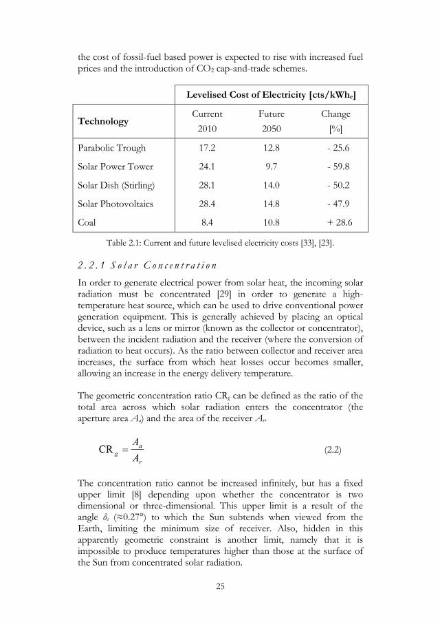
The levelised cost of electricity from solar thermal power plants has been shown to be amongst the most competitive of all renewable energy technologies [33], with a significant cost advantage over solar photovoltaics when deployed on a large scale. However, solar thermal technology has not yet matured to the point of grid-parity with conventional power generation systems, although this is predicted to occur within the next 15 years [23]. Rapid reductions in the levelised cost of solar thermal systems are expected, as shown in Table 2.1, whereas

25

the cost of fossil-fuel based power is expected to rise with increased fuel prices and the introduction of CO2 cap-and-trade schemes.

Levelised Cost of Electricity [cts/kWhe]

Technology Current

2010

Future

2050

Change

[%]

Parabolic Trough 17.2 12.8 - 25.6

Solar Power Tower 24.1 9.7 - 59.8

Solar Dish (Stirling) 28.1 14.0 - 50.2

Solar Photovoltaics 28.4 14.8 - 47.9

Coal 8.4 10.8 + 28.6

Table 2.1: Current and future levelised electricity costs [33], [23].

2 . 2 . 1 S o l a r C o n c e n t r a t i o n

In order to generate electrical power from solar heat, the incoming solar radiation must be concentrated [29] in order to generate a high-temperature heat source, which can be used to drive conventional power generation equipment. This is generally achieved by placing an optical device, such as a lens or mirror (known as the collector or concentrator), between the incident radiation and the receiver (where the conversion of radiation to heat occurs). As the ratio between collector and receiver area increases, the surface from which heat losses occur becomes smaller, allowing an increase in the energy delivery temperature.

The geometric concentration ratio CRg can be defined as the ratio of the total area across which solar radiation enters the concentrator (the aperture area Aa) and the area of the receiver Ar.

r

a

gA

ACR (2.2)

The concentration ratio cannot be increased infinitely, but has a fixed upper limit [8] depending upon whether the concentrator is two dimensional or three-dimensional. This upper limit is a result of the angle δs (≈0.27°) to which the Sun subtends when viewed from the Earth, limiting the minimum size of receiver. Also, hidden in this apparently geometric constraint is another limit, namely that it is impossible to produce temperatures higher than those at the surface of the Sun from concentrated solar radiation.

26

The level of temperature that is produced at the solar receiver is a function of a number of parameters, including the concentration ratio and the material properties of the receiver itself. Assuming that radiation losses are dominant [29], the maximum conceivable receiver temperature Tmax is given by (2.3) where ηo is the optical efficiency of the solar collector, α and ε the material absorptivity and emissivity respectively, σ the Stefan-Boltzmann constant and Io the direct normal irradiation on-site.

4max o

g

o ICR

T

(2.3)

It can be seen from (2.3) that in order to raise the heat delivery temperature a number of parameters can be modified. Increasing the concentration ratio is one option as well as increasing the ratio of α to ε of the receiver material: increasing the ‘selectiveness’ of the surface. Whilst selectivity is a powerful tool, the most usual means [29] of increasing the energy delivery temperature is increasing the concentration ratio. Maintaining a high optical efficiency of the collector is also important for high-temperature systems and, as always, a solar collector performs between in areas with higher direct normal irradiation [22].

Concentration systems present the drawback that they can only harness the beam radiation component of the solar flux [32], and as such the radiation arriving at the Earth’s surface in diffuse form is automatically wasted. The angle of incidence of the beam radiation on the collector is of great importance and, as such, the concentration system must constantly track the Sun to maintain the correct alignment. The tracking motion to be performed will depend of the nature of the collector, but a high degree of precision is required to ensure effective concentration.

2 . 2 . 2 L i n e a r C o n c e n t r a t i o n D e v i c e s

Linear concentration focuses the Sun’s rays in two dimensions onto a receiver placed at the focus, which takes the form of a line. The system tracks the Sun’s movement about a single axis to maintain the alignment between the incident rays and the linear axis of the collector. For two-dimensional concentration, the upper limit on the concentration ratio [29] is given by (2.4) where L is the distance of the Earth from the Sun, and Rs the radius of the Sun.

212sin

1CR 2

max ss

D

R

L

(2.4)

27

The most common linear concentration device is the parabolic trough collector, shown in Figure 2.4. Practical devices achieve concentration ratios between 30 and 100. Solar field outlet temperatures are limited to between 300°C and 400°C, mainly by the thermal stability of the heat transfer fluid [22].

Figure 2.4: Parabolic trough linear concentration device. Source: RISE Information Portal, 2004

Figure 2.5: Heliostat field point focus concentration device. Source: RISE Information Portal, 2004

2 . 2 . 3 P o i n t F o c u s C o n c e n t r a t i o n D e v i c e s

Point focusing systems concentrate the Sun’s rays to a central receiver placed at the punctual focus point, achieving three-dimensional concentration. A two-axis tracking system is necessary to maintain the aperture of the collector aligned with the direction of the Sun’s rays. For a three dimensional concentration system, the upper limit of concentration ratio [29] is given by (2.5).

28

45000sin

1CR

22

23

max ss

D

R

L

(2.5)

Whilst being theoretically possible, the higher concentration ratios are incredibly difficult to produce physically, and the current range of realisable concentration ratios extends from about 500 for commercial systems to above 5000 for experimental dishes [22].

2 . 3 S o l a r T h e r m a l P o w e r P l a n t s ( P a p e r 1 )

The key challenges and opportunities facing solar thermal power plants in the near future are presented in Paper 1, which also gives an overview of the importance of solar power technology to the Swedish industrial and research communities.

The vast majority of contemporary utility-scale solar thermal power plants are based on Rankine cycle (steam-turbine) technology [22]. They operate towards the lower end of the range of concentration ratios and achieve receiver temperatures up to around 400°C [25]. The power block therefore consists of conventional steam-cycle technology, which was seen as presenting a lower risk when developing the first generation of solar power plants. The lower operating temperature also facilitates the integration of thermal energy storage, which allows an increase in the capacity factor and dispatchability of the power plant.

Two main collector technologies are currently employed in solar thermal power plants: parabolic trough and central receiver technologies, as shown in Figure 2.6 and Figure 2.7 respectively. Apart from the collector technology, the key difference [29] between these two power plant concepts lies in the working fluid of the solar receiver: thermal oil for the troughs and water or air for the central receivers.

Parabolic troughs are undisputedly the most mature of the solar thermal power technologies, with power plants in commercial operation since the early 1980s. Central receiver (or power tower) technology is an emerging concept which presents the possibility to reach higher concentration ratios and thus higher temperatures at the receiver. The first commercial power tower plants have recently been deployed in Spain [25].

In a conventional parabolic trough solar power plant, a liquid heat transfer medium (usually thermal oil) circulates through the solar collector field, where it is heated to the desired temperature. The hot heat transfer fluid is then sent to a steam generator where it produces live steam for the Rankine-cycle at pressures of around 100 bar and

29

temperatures up to 400°C [25]. In some plants, a thermal energy storage system operates in parallel to the collector field, allowing excess solar energy to be stored for use when the solar flux becomes insufficient. The energy storage medium is not necessarily the same as that used in the collector field; contemporary power plants predominantly use molten-salts for thermal energy storage.

Figure 2.6: Layout of a parabolic trough solar thermal power plant Source: Deutsches Zentrum für Luft- und Raumfahrt

Figure 2.7: Layout of a central receiver solar thermal power plant. Source: Deutsches Zentrum für Luft- und Raumfahrt

An alternative to the parabolic trough solar power plant is the central receiver system, in which a field of heliostats focuses the Sun’s rays to a receiver placed at the top of a central tower. This receiver converts the Sun’s energy into heat; either raising steam directly (as is the case for the

30

PS10 power plant) or heating air for use in a steam boiler (demonstrated at the KAM Jülich solar tower). In principal, the power block remains the same as that used in other solar thermal power systems.

Central receiver systems have the potential for significantly higher solar-electric conversion efficiencies due to the fact that higher temperatures can be reached at the receiver. The technology remains in its early stages however, with only a handful of power plants having been built and tested across the world. Today the optimal thermal power from a tower seems to be around 100 MWth with a 160 m tower and some 830 heliostats with a 121 m2 mirror area per unit [22]. Larger systems can be expected considering possible advancement in mirror and receiver design and control system precision.

2 . 4 A n d a s o l 1 S o l a r P o w e r P l a n t

The power plant under study in this work is Solar Millenium’s Andasol 1, a state of the art parabolic trough solar thermal power plant located at 37.1°N near the town of Aldiere in Spain [25]. Like the SEGS and Nevada Solar One plants, the Andasol 1 facility is based around a conventional parabolic trough collector field with thermal oil as the heat transfer fluid and a two-tank molten-salt based storage system. The power block comprises a reheat steam-cycle driving a 50 MWe Siemens SST-700RH steam-turbine.

The Andasol 1 plant was the first European parabolic trough power plant. Located at an altitude of 1’100 m above sea level, the site experiences excellent insolation, with an annual total above 2’100 kWh/m2. An aerial view of the plant is shown in Figure 2.8.

Figure 2.8: Solar Millenium Andasol 1 power plant.

31

An indirect two-tank thermal energy storage system capable of holding 28’500 tons of molten salts (more precisely a eutectic mixture of potassium and sodium nitrate) allows the power plant to be run at full capacity for a duration of 7.5 hours [25]. The Andasol 1 power plant is currently used to meet summer peak electricity demand in the Spanish power grid, caused primarily by air conditioning units, a task to which solar power plant are ideally suited as the cooling demand and insolation are generally in phase.

A certain amount of information about the Andasol 1 power plant is provided in Table 5.

Developer / Owner ACS Cobra Group

Production Started 2008

Turbine Capacity 50 [MWe]

Annual Production 158’000 [MWh]

Solar-Field Aperture 510’000 [m2]

Solar Resource 2’136 [kWh/m2/yr]

Solar Field Temperature 393 [°C]

Table 2.2: Andasol 1 power plant overview. Source: IEA SolarPACES Annual Report 2008 [25]

32

33

3 Transient Modell ing of Solar Steam Turbines

In order to evaluate methods for increasing the operational flexibility of steam-turbines in solar thermal power plants, a detailed thermal model of a solar steam-turbine has been established. The key purpose of the model is the prediction of the metal temperatures within the turbine, both during operation and stand-by, in order to determine start-up speeds. To achieve this, the steam-turbine is simulated using a coupled model, composed of three interconnected parts:

1. A finite-volume heat conduction model to evaluate the casing and rotor metal temperatures.

2. A thermodynamic model to determine the steam expansion temperatures during operation, along with the corresponding heat transfer coefficients.

3. A separate gland steam network model to calculate the temperatures and heat fluxes in the labyrinth joints.

The steam-turbine model has been developed using MATLAB classes in order to allow integration with an existing in-house tool [27] for the dynamic simulation and optimisation of solar thermal systems.

3 . 1 F i n i t e V o l u m e M o d e l

3 . 1 . 1 H e a t C o n d u c t i o n E q u a t i o n

Heat conduction in solid materials is governed by Fourier’s law [12], which links the local heat flux to the temperature gradient within the material, by means of the thermal conductivity k of the conductive medium. For an isotropic solid this gives the equation (3.1) where q is the local heat flux vector, x the position vector and T the temperature field within the material. For highly conductive materials, the variation of k as a function of T can, in practice, be neglected. In layman’s terms, this law states that heat flows from areas of high temperature to areas of low temperature and that the rate of heat transfer increases with the temperature gradient, proportional to the thermal conductivity.

txTxktxTTxktxq ,,,,

(3.1)

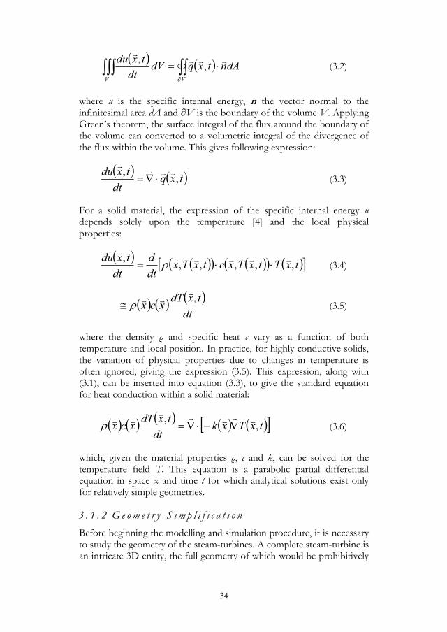
The first law of thermodynamics [4] can also be applied within the material and it states that the net flux of energy into a particular volume V is equal to the change in internal energy of that volume (3.2).

34

V V

dAntxqdVdt

txdu

,,

(3.2)

where u is the specific internal energy, n the vector normal to the infinitesimal area dA and ∂V is the boundary of the volume V. Applying Green’s theorem, the surface integral of the flux around the boundary of the volume can converted to a volumetric integral of the divergence of the flux within the volume. This gives following expression:

txqdt

txdu,

,

(3.3)

For a solid material, the expression of the specific internal energy u depends solely upon the temperature [4] and the local physical properties:

txTtxTxctxTxdt

d

dt

txdu,,,,,

,

(3.4)

dt

txdTxcx

,

(3.5)

where the density ρ and specific heat c vary as a function of both temperature and local position. In practice, for highly conductive solids, the variation of physical properties due to changes in temperature is often ignored, giving the expression (3.5). This expression, along with (3.1), can be inserted into equation (3.3), to give the standard equation for heat conduction within a solid material:

txTxkdt

txdTxcx ,

,

(3.6)

which, given the material properties ρ, c and k, can be solved for the temperature field T. This equation is a parabolic partial differential equation in space x and time t for which analytical solutions exist only for relatively simple geometries.

3 . 1 . 2 G e o m e t r y S i m p l i f i c a t i o n

Before beginning the modelling and simulation procedure, it is necessary to study the geometry of the steam-turbines. A complete steam-turbine is an intricate 3D entity, the full geometry of which would be prohibitively

35

complex to model as part of this MATLAB-based study, requiring instead the use of commercial FEM codes.

In order to facilitate the study of the solar steam-turbine, a 2D axisymmetric model will be considered, which will require the simplification of the full turbine geometry. In an axisymmetric model, only two cardinal axes are considered, namely the axial direction z and the radial direction r, all phenomena are assumed to be invariant in the tangential direction φ. The cylindrical coordinate system is used in an

axisymmetric model and, as such, the Cartesian gradient operator is

replaced with the cylindrical gradient operator :

zrr ez

er

er

1 (3.7)

where ê is the unit vector for the cardinal axes.

Within the turbine, the blade disks form a region of very convoluted geometry with protruding surfaces and gaps between adjacent disks, as shown in Figure 3.1. To model the full detail of the geometry in this region is out of the scope of this work, instead the rotor and casing are modelled using two distinct domains in order to simplify calculation of the blade disk area.

Figure 3.1: Complex geometry of the blade disk regions.

The central part of the rotor is considered to be solid metal and is thus modelled using the isotropic heat flux law presented in equation (3.1). The blade disk region is also modelled as a continuous domain, ignoring the intra-disk gaps, but with a reduced density and a non-isotropic thermal conductivity to take into account the preferential direction of heat transfer introduced by the disks.

Within a non-isotropic domain, Fourier’s law (3.1) must be modified to take into account the different thermal conductivities of the material in

36

the different directions. The scalar thermal conductivity k is replaced with the thermal conductivity matrix K, which is a diagonal matrix containing the different values of the thermal conductivity along the cardinal axes.

txTxKtxq ,,

(3.8)

with

z

y

x

k

k

k

K

00

00

00

In the axisymmetric case considered here, only the axial ka and radial kr thermal conductivities need to be considered:

trzT

rzk

rzktrzq r

r

a,,

,0

0,,,

(3.9)

The blade disks themselves are comprised of metal, with high thermal conductivity km, whereas the gap between adjacent blades is filled with steam, with very low thermal conductivity ks. These two terms can differ by several orders of magnitude and it is the different paths of heat conduction in the axial and radial directions that leads to the anisotropy in this region. For the steam trapped within the gap between adjacent disks, Couette flow [12] is assumed due to the narrowness of the gap.

In the axial direction, the two thermal resistances (metal and steam) are in series and thus even with only a small gap, the low thermal conductivity of the steam serves to greatly reduce the overall conductivity in this direction. If the axial steam-gap fraction is defined as ε, the equivalent axial conductivity ka can be determined using:

msa kkk

11 (3.10)

On the other hand, in the radial direction, the two thermal resistances are in parallel and, as such, the low thermal conductivity of the steam will only slightly reduce the overall conductivity in this direction if the blade gap fraction is small.

msr kkk 1 (3.11)

37

The same reasoning has been applied to the casing and stator disks, and the same relationships hold. As a result of these simplifications, the differential equation being solved to determine the temperature profiles within the turbine metal is (3.12) where T, the temperature profile, is a function of the axial position, the radial position and time, and the thermal conductivity matrix K changes as a function of position.

trzTrzKdt

trzdTrzcrz rr ,,,

,,,,

(3.12)

3 . 1 . 3 F i n i t e V o l u m e T e c h n i q u e s

Due to the complex geometry and discontinuous physical properties of the solar steam-turbine, no analytical solution exists for the heat conduction equation presented in the previous section. As such, the finite volume method will be applied, which serves to convert the partial differential equation (3.12) into a series of algebraic expressions which are easier to solve.

Under the finite volume approach, the temperature field is not evaluated continuously but rather at a number of discrete points, or ‘nodes’ within the domain. The method gets its name from the fact that the equations are evaluated for each point within the small ‘finite’ volume around each node.

The finite volume technique is elaborated based on the generalised form of the heat conduction equation, which states that:

txqdt

txdTxcx ,

,

(3.13)

By integrating this expression within the finite volume V around each node equation (3.14) is obtained, similar in form to expression (3.2) presented previously.

V V

dAntxqdVdt

txdTxcx

,

, (3.14)

By considering the average values within the finite volume i and across each bounding surface ij, the integrative terms can be reduced to a scalar

expression at each node, giving (3.15) where ̅, ̅ and ̅ are respectively the mean density, specific heat and temperature of the volume. The

mean flux ̅ across the bounding surface Aij between nodes i and j is

determined using Fourier’s law (3.1).

38

n

j

ijiji

iii Aqdt

TdVc

1

(3.15)

As the flux leaving the cell i is equal to the flux entering cell j, the finite volumetric technique inherently satisfies the laws of conservation, and the method is said to be conservative [26].

The resolution of the time differential in equation (3.15) can be done using any number of appropriate schemes. First order schemes are quicker and require less memory than higher order schemes [7] and are often chosen for these reasons. However, if a greater degree of precision is required, second, third or even fourth order schemes can be used. The first order approximation of the time differential is given by (3.16) where n is the current timestep and n+1 the next timestep.

t

TTtO

t

TT

dt

dT nnnn

11

(3.16)

The error of a first order approximation decreases linearly with reductions in the timestep.

3 . 1 . 4 B o u n d a r y C o n d i t i o n s

In addition to elaborating the equation system to be solved within the simulation domain, it is also necessary to define the limiting conditions that occur at the boundaries of the domain. These source terms will be crucial to determine the direction of the heat fluxes within the turbine.

All boundary conditions in this work are of the Neumman or Robin types [7], meaning that the temperatures themselves are not imposed anywhere within the model. Neumann boundary conditions impose a fixed value for the flux at a boundary and are used in this model to represent the symmetry lines and other non-conducting boundaries. Robin boundary conditions impose a heat flux based on the boundary temperature and are used to represent the convection heat transfer occurring within the model.

The external heat fluxes qb along the convective boundaries can be calculated using the generic equation (3.17) where Tb is the temperature of the boundary node, αb the heat transfer coefficient at the boundary, and Text the external temperature at the boundary.

extbbb TTq (3.17)

39

The heat flux across the boundary between the external edge of the casing and the environment results from composite heat transfer through the insulation layer and a natural convection layer. The thermal capacity of the insulation layer is neglected in this study as the conduction resistance dominates over the effects of thermal inertia, which is an order of magnitude below that of the metal regions in any case. The heat flux at the insulation boundary can therefore be determined using:

ncins

ins

abb

k

e

TTq

1

(3.18)

where eins is the thickness of the insulation layer, kins its thermal conductivity, αnc the external natural convection heat transfer coefficient and Ta the ambient temperature. Morel [19] recommends a value of 8 W/m2K for natural convection from a hot surface inside a building.

Within the blade passage, the thermal inertia of the blades themselves is not taken into account during calculation, as their mass is significantly less than that of the disks and other solid parts. Instead, the blades are considered as ‘fins’, augmenting the convective heat transfer that occurs within the passage [12]. With respect to the basic boundary surface area, the heat flux of the extended surface can be calculated using:

stbfobb TTq (3.19)

where the terms ηo and φf are respectively the overall surface efficiency and the surface multiplication factor of the finned surface. These terms take into account the heat transfer augmentation due to the extended surface, as the calculation of the flux at the boundary refers to the base heat transfer area and not the total heat transfer area.

3 . 2 S t e a m E x p a n s i o n M o d e l

To be able to calculate the heat transfer within the flow passages, it is necessary to resolve the steam temperature and pressure profiles within the blade passage of each turbine unit. In order to be able to achieve this by applying Stodola’s ellipse law [6], the turbine is divided into a number of segments between the steam extraction points, as shown in Figure 3.2, within which ellipse constants Y can be calculated. The nominal isentropic efficiencies ηs are specified by the manufacturer for each segment.

40

Figure 3.2: Input and boundaries of the steam-turbine model, including segments for Stodola modelling.

3 . 2 . 1 S t o d o l a E x p a n s i o n M o d e l

The off-design operation of a multi-stage axial turbine can be modelled using Stodola’s ellipse [6], which relates the mass flow coefficient Φ to the pressure ratio across the unit. The mass flow coefficient at any point within the expansion can be determined using (3.20) where M is the mass flow through the given section, P the pressure, ρ the fluid density and T the absolute temperature [4] corresponding to the state point in the given section.

P

TM

P

M

(3.20)

For each expansion section with a given backpressure Pout, a simple relationship may be developed [6], allowing the expansion to be considered as if it were a nozzle. Known as Stodola’s ellipse, this relationship implies that:

2

1

P

Pout (3.21)

Graphically, this relationship can be presented as shown in Figure 3.3. Although valid over a wide range of pressure ratios, Stodola’s ellipse does not accurately predict the mass flow once choking begins [6]. Below the critical backpressure Pt, sonic flow conditions occur within the section and the ellipse law does not hold. A fixed value of the mass flow constant can be assumed during choking, as shown in Figure 3.3, and this correction to the ellipse law is relatively easy to put into practice in the simulation models.

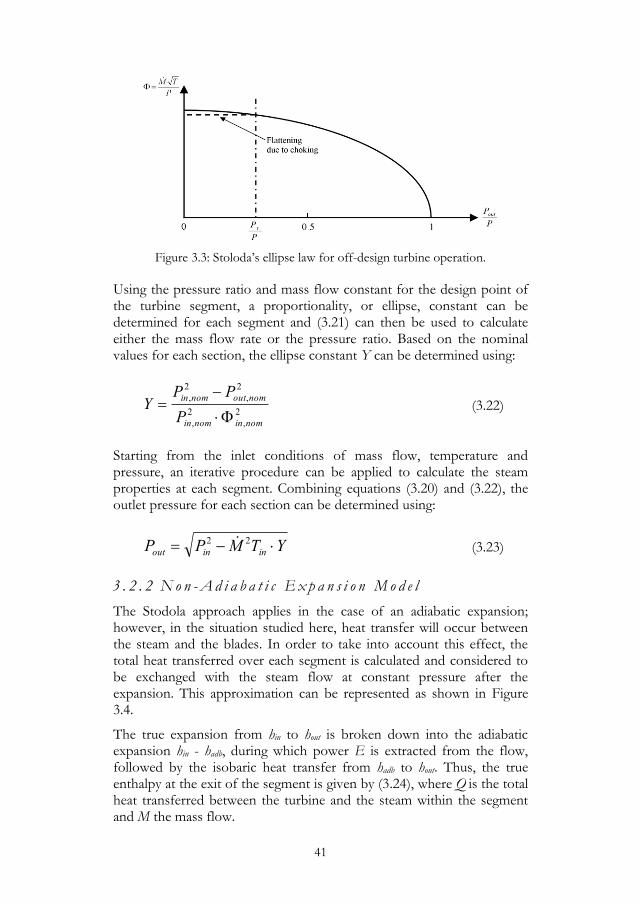
41

Figure 3.3: Stoloda’s ellipse law for off-design turbine operation.

Using the pressure ratio and mass flow constant for the design point of the turbine segment, a proportionality, or ellipse, constant can be determined for each segment and (3.21) can then be used to calculate either the mass flow rate or the pressure ratio. Based on the nominal values for each section, the ellipse constant Y can be determined using:

2

,

2

,

2

,

2

,

nominnomin

nomoutnomin

P

PPY

(3.22)

Starting from the inlet conditions of mass flow, temperature and pressure, an iterative procedure can be applied to calculate the steam properties at each segment. Combining equations (3.20) and (3.22), the outlet pressure for each section can be determined using:

YTMPP ininout 22 (3.23)

3 . 2 . 2 N o n - A d i a b a t i c E x p a n s i o n M o d e l

The Stodola approach applies in the case of an adiabatic expansion; however, in the situation studied here, heat transfer will occur between the steam and the blades. In order to take into account this effect, the total heat transferred over each segment is calculated and considered to be exchanged with the steam flow at constant pressure after the expansion. This approximation can be represented as shown in Figure 3.4.

The true expansion from hin to hout is broken down into the adiabatic expansion hin - hadb, during which power E is extracted from the flow, followed by the isobaric heat transfer from hadb to hout. Thus, the true enthalpy at the exit of the segment is given by (3.24), where Q is the total heat transferred between the turbine and the steam within the segment and M the mass flow.

42

Figure 3.4: Steam expansion h-s diagram, showing the different terms involved in the temperature calculations.

M

Q

M

Ehh inout

(3.24)

The calculation of hadb requires knowledge of the isentropic efficiency ηs of the segment. Based on the nominal value ηso provided by the manufacturer, the off-design efficiencies can be calculated using a correlation (3.25) proposed by Ray [24], where N is the rotational speed of the unit and Δhs the isentropic enthalpy variation.

2

12

s

so

o

sosh

h

N

N (3.25)

3 . 2 . 3 H e a t T r a n s f e r C a l c u l a t i o n

The heat transfer coefficients within the flow passages are calculated based on nominal values specified by the turbine manufacturer, shown in Figure 7.

Figure 3.5: Nominal flow passage heat transfer coefficients.

The off-design values are calculated using a correlation (3.26) also provided by the turbine manufacturer, where Tin is the inlet temperature, Pin and Pout are the inlet and outlet pressures respectively and Π = Pout/Pin

43

is the pressure ratio across the section. The subscript o refers to the design values.

8.0

2

28.0

1

1

o

in

o

in

in

o

in

oo T

T

P

P

M

M

(3.26)

3 . 3 G l a n d S t e a m N e t w o r k M o d e l

In order to prevent the infiltration of air within the turbines, the labyrinth joints must be provided with an external supply of steam (known as gland steam) during idle periods and low-load operation. This is shown schematically in Figure 3.6. It is also necessary to provide gland steam to the low-pressure-side labyrinth of the low-pressure turbine even during full-load operation, due to the vacuum conditions found within the condenser.

Figure 3.6: Steam-turbine rotor showing gland steam injection

The boundary heat flux q within the labyrinth joints is modelled (3.27) assuming a heat exchange effectiveness ε [12] for the heat transfer between the gland steam temperature Tgst and the surface metal temperature Tm, where G is the mass flux through the labyrinth and cp the average heat capacity of the steam between the two temperatures.

mgstp TTGcq (3.27)

The external gland steam network provides two levels of steam for injection into the labyrinths on either the high-pressure or low-pressure side, with potentially a different temperature for each. When the turbine is idle, the gland steam temperature is fixed entirely by the external supply. During part-load operation, the temperature of the gland steam is determined by the mixing of the externally supplied steam and the internal steam leakage from the inlet and exhaust cavities. The fraction of the gland steam delivered by the external supply is shown in Figure 3.7

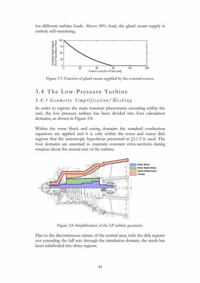
44

for different turbine loads. Above 60% load, the gland steam supply is entirely self-sustaining.

Figure 3.7: Fraction of gland steam supplied by the external source.

3 . 4 T h e L o w - P r e s s u r e T u r b i n e

3 . 4 . 1 G e o m e t r y S i m p l i f i c a t i o n / M e s h i n g

In order to capture the main transient phenomena occurring within the unit, the low pressure turbine has been divided into four calculation domains, as shown in Figure 3.8.

Within the rotor block and casing domains the standard conduction equations are applied and it is only within the rotor and stator disk regions that the anisotropic hypothesis presented in §3.1.2 is used. The four domains are assumed to maintain constant cross-sections during rotation about the central axis of the turbine.

Figure 3.8: Simplification of the LP turbine geometry.

Due to the discontinuous nature of the central area, with the disk regions not extending the full way through the simulation domain, the mesh has been subdivided into three regions.

45

The central grid contains four layers: the rotor block, the two disk regions and the casing, whereas the left and right grids contain only rotor and casing layers. This is shown in Figure 3.9, and it can be seen that the use of a structured grid allows the cells to be well aligned with the geometry of the turbine model.

Figure 3.9: Mesh grid for the LP turbine model

3 . 4 . 2 B o u n d a r y C o n d i t i o n s

Based on the geometry mesh presented in Figure 3.9, the boundary conditions shown in Figure 3.10 can be defined for the low-pressure steam-turbine model. Two types of boundary condition can be distinguished: insulation boundaries with no heat flux (Neumann-type) and convection boundaries (Robin-type), for which a heat transfer coefficient and external temperature must be defined [7]. The heat transfer coefficients used in the model have been obtained via an internal communication from Siemens Industrial Turbomachinery. The nominal heat transfer coefficients within the blade passage were shown for both the LP and HP turbines in Figure 3.5.

The external boundary condition consists of a composite heat transfer term, with conduction through the insulation blankets followed by natural convection out to the atmosphere. This heat flux can be calculated using (3.18) and a specified value of the ambient temperature. An insulation thickness of 100mm can be assumed for the thermal blankets, with the temperature-dependant thermal conductivity given in Figure 3.11.

46

Figure 3.10: Boundary conditions for the LP turbine model.

The data on the thermal insulation conductivity was obtained via a corporate communication from Roxull, Brandsäker Isolering, see the Appendix.

Figure 3.11: Insulation blanket thermal conductivity.

3 . 5 T h e H i g h - P r e s s u r e T u r b i n e

3 . 5 . 1 G e o m e t r y S i m p l i f i c a t i o n / M e s h i n g

In order to capture the main transient phenomena occurring within the unit, the high-pressure turbine has also been divided into four calculation domains, as shown in Figure 3.12.

As was the case for the low-pressure turbine, the disk regions do not extending the full way through the simulation domain and as such the mesh has been subdivided into three regions. The central grid contains five layers: the rotor block, the two disk regions the stator mounting and the casing, whereas the left and right grids contain only rotor and casing layers. This is shown in Figure 3.13.

47

Figure 3.12: Simplification of the HP turbine geometry.

Figure 3.13: Mesh grid for the HP turbine model

Figure 3.14: Boundary conditions for the HP turbine model

48

3 . 5 . 2 B o u n d a r y C o n d i t i o n s

Based on the geometry mesh presented in Figure 3.13, the boundary conditions shown in Figure 3.14 can be defined for the high-pressure steam-turbine model. As was the case for the LP turbine, two types of boundary condition can be distinguished: insulation boundaries with no heat flux and convection boundaries.

3 . 6 M o d e l V a l i d a t i o n

Before the results of the steam-turbine models can be used to make predictions and suggest improvements it is necessary to validate the output of the model against measured data. If necessary, the model can then be ‘tweaked’ in order to ensure a more accurate representation of the physical reality. Data for validation of the steam-turbine models has been obtained courtesy of Dr. Markus Jöcker at Siemens Industrial Turbomachinery from measurements taken at the Andasol 1 parabolic trough plant near Aldiere in Spain. Operational data for the turbine was measured during a period of 4 days (96 hours) from the 21st to the 25th October 2009.

3 . 6 . 1 V a l i d a t i o n D a t a

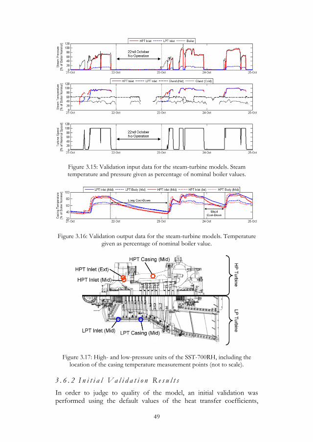
The values presented in the following graphs are used as input to the steam-turbine models during validation. The measured values of the live steam pressure at the boiler outlet and high- and low-pressure turbine inlets are shown in Figure 3.15. It can be seen that the turbine was not operated at all during the 22nd October and that a number of starts and stops occurred on the other days. The wide variety of operating conditions experienced by the turbines during the measurement period allows the dynamics of the model to be validated across a nearly complete range of situations likely to be encountered, namely start-up, short cool-down (<10h), long cool-down (>24h) and load variation. In addition, Figure 3.15 also shows the evolution of the different steam temperatures as well as the turbine speed during the validation period.

The measured turbine casing temperature values are shown in Figure 3.16. It is against these values that the output of the simulation model will be validated. The locations of the temperature sensors used to obtain the values for the casing measurements are shown in Figure 3.17. The temperature measurement points at the turbine inlet are instrumented by default in steam-turbines of this type, whereas the additional casing measurements were taken to assist in this, and other, studies.

49

Figure 3.15: Validation input data for the steam-turbine models. Steam temperature and pressure given as percentage of nominal boiler values.

Figure 3.16: Validation output data for the steam-turbine models. Temperature given as percentage of nominal boiler value.

Figure 3.17: High- and low-pressure units of the SST-700RH, including the location of the casing temperature measurement points (not to scale).

3 . 6 . 2 I n i t i a l V a l i d a t i o n R e s u l t s

In order to judge to quality of the model, an initial validation was performed using the default values of the heat transfer coefficients,

50

physical properties and efficiencies presented in §3.4 and §3.5. The model was run with a timestep of 5 minutes, equal to that of the measurement devices, thus eliminating the influence of interpolation of the input data on the results.

A first comparison of the measured and simulated low- and high-pressure turbine temperatures is shown in Figure 3.18. The thick coloured lines represent the output values from the simulation, whereas the thinner black lines are the corresponding values from the measurements.

Figure 3.18: Initial comparison of the measured and simulated temperatures

It can be seen in Figure 3.18 that the general trends in the measurement data for the low-pressure turbine are followed by the simulation output. However, the simulation shows a tendency to under-predict the measured values. Especially during the cool-down phases, the temperature values given by the model drop too rapidly, indicating that the rate of heat loss is too high.

In the case of the high-pressure turbine, it can be seen in that the general trends in the measurement data are also respected by the simulation output. However, the simulation shows a tendency to over-predict the measured values. During the cool-down phases, the temperature of the casing measurement point remains too high; the inlet measurement is predicted with a much greater degree of accuracy. It can be concluded that the rate of heat loss from the high-pressure turbine is not correctly distributed within the model.

A more qualitative evaluation of the accuracy of the model’s predictions can be obtained by examining the relative error between the measured

51

and simulated values. This error is shown at the bottom of Figure 3.18 for all four measurement points. The tendency for the HP-turbine model to over-predict the temperature values can clearly be seen, as well as the tendency of the LP-turbine model to under-predict the values. Overall the performance of the model in its initial form gives an average relative error of 4.1%, with a maximum value of 18.3% for HP-turbine model and 14.1% for the LP-turbine model. These large maximum errors are especially worrying given that they occur at the end of the cool-down period: it is the prediction of the temperature at this time that will determine the allowable turbine start-up speed.

The performance of the model in its initial state is therefore not sufficient to allow detailed predictions to be made about the start-up and cool-down behaviour of the solar steam-turbine. In order to rectify this, and improve accuracy of the predictions, a number of key parameters in the model will be ‘tweaked’, using a population-based genetic optimisation algorithm.

3 . 6 . 3 M o d e l P a r a m e t e r C o r r e c t i o n

As the model does not give sufficiently accurate results in its initial form, it will be necessary to adjust a number of parameters in order to obtain more reliable results. A multi-objective optimisation technique based on an evolutionary algorithm [14] will be used to minimise the model error through the selection of a number of correction factors.

In the models presented in §3.1 to §3.5, the data values with the highest degree of uncertainty are the heat transfer coefficients, and as such it is these values which are selected as prime candidates for adjustment. In total, 10 different correction terms will be used to modify the heat transfer coefficients in both the high- and low-pressure steam-turbines, as shown in Table 3.1.

Based on the value selected for the correction factor, the new values of the nominal heat transfer coefficients are calculated using:

corrf

ocorr 10 (3.28)

where αcorr is the heat transfer term, αo the unmodified term and fcorr the applicable correction term from. According to the limits fixed in Table 3.1, this equation scales the heat transfer terms by an order of magnitude in each direction. A power-based formulation was chosen in order to ensure that the optimiser gives equal consideration to scaling of the coefficients in both directions.

52

# Factor Affected Heat Transfer Terms Range

1 fcond Flow Passage Conduction -1, +1

2 flabyrinth Gland Steam Effectiveness -1, 0

3 fbear Bearing Oil Convection -1, +1

4 fLPst LP Turbine Flow Passage -1, +1

5 fLPcav LP Turbine Inlet Cavity

LP Turbine Exhaust -1, +1

6 fLPext LP Turbine Heat Losses -1, +1

7 fHPst HP Turbine Flow Passage -1, +1

8 fHPcav HP Turbine Inlet Cavity

HP Turbine Exhaust -1, +1

9 fHPextr HP Turbine Extraction Cavity -1, +1

10 fHPext HP Turbine Heat Losses -1, +1

Table 3.1: Steam-turbine heat transfer coefficient correction factors.

The main objective of the optimisation will clearly be to minimise the error between the measured values and those given by the simulation. As such, the first objective considered will be the minimisation of the average relative error εrel, defined as:

N

n mes

messim

reltnT

tnTtnT

N 1

1 (3.29)

where N is the total number of measurement-points/simulation-timesteps, Δt the measurement/simulation timestep and Tsim and Tmes are respectively the simulated and measured values of the temperature at each timestep.

However, it is also assumed that the heat transfer data provided by the manufacturer is of high quality and should be trusted wherever possible. As such, a second objective will be fixed as the minimisation of the absolute magnitude Mcorr of the correction, defined as:

12

1i

corrcorr fM (3.30)

The minimisation of these two objective functions will be conflicting as the average absolute error will decrease as the magnitude of the correction increases; a multi-objective algorithm is therefore well adapted to study a problem of this nature [14].

53

The algorithm population after 600 model evaluations is shown in Figure 3.19, along with the position of the Pareto-optimal front [14]. A point can be defined as being Pareto-optimal if there exists no other point within the decision space that is better in all objectives. By choosing a solution on the Pareto front, naïve solutions are avoided and, of all the feasible solutions, only those that satisfy as best as possible all objectives are considered.

Figure 3.19: Evolutionary algorithm population after 600 evaluations. Position of the Pareto-optimal front shown in red.

Point 1 in Figure 3.19 is the Pareto-optimal point with the lowest relative error, but it displays a very high correction magnitude. For this study, the correction factor values from Point 2 are chosen. This Pareto-optimal point maintains a low relative error (at 1.2% average error) but sits before the inflection point on the Pareto curve, giving a much lower correction magnitude and thus more confidence in the model.

3 . 6 . 4 F i n a l V a l i d a t i o n R e s u l t s

The evolution of the relative error between the temperature measurements and the simulated values is shown in Figure 3.20, along with a more direct comparison between the measured and simulated casing temperatures. It can be seen that, unlike in §3.6.2, the largest values of the relative error now occur during the start-up phases, where the most rapid changes in operating condition occur. The peak relative error during these phases is 7.5%, during the cool-down phases it is considerably lower. The transient behaviour of interest in the solar steam-turbine units can thus be considered to be well captured.

A certain degree of uncertainty persists regarding the rotor temperatures, due to the lack of any validation data for the turbine rotors and the difficulty of evaluating analytically the rate of heat transfer across the blade passage when the turbine is idle. Access to reliable temperature

54

measurements for the rotor would greatly improve the quality of these predictions.

Figure 3.20: Comparison between simulated values and measured data for the optimised steam-turbine models. Thick coloured lines show simulated values,

thin black lines show measurements. Temperatures given as percentage of nominal boiler temperature.

3 . 6 . 5 S e n s i t i v i t y A n a l y s i s

As a number of correction factors were applied in order to obtain these validation results, it is also necessary to examine the sensitivity of the turbine model to the corrections applied.

Figure 3.21: Correction factor magnitudes and sensitivity of the measured temperatures to a ±25% change in correction factor.

The results of this analysis are presented in Figure 3.21 which shows the values of the correction factors used, alongside their maximum influence

55

on the measured temperatures within a ±25% range around the selected value. The correction factor numbers correspond to those in Table 3.1.

The first two influence bars in Figure 3.21 show the maximum change in the measured casing and rotor temperatures during the whole simulation period. The second two bars give the maximum change in casing and rotor temperature measured just before start-up. It is this second set of temperatures that are crucial for the determination of the start-up speed.

With a ±25% variation in the correction values, it can be seen that the maximum influence on the simulated temperatures is below 3%, and the influence on the key pre-start-up temperatures is below 2%. Globally, it can be seen that the pre-start-up temperatures are relatively insensitive to changes in the correction factors applied to the model. Concerning the difficulty in determining the rotor-casing heat transfer, it is reassuring to see that the influence of this correction factor (#1) is negligible.

56

57

4 Dynamic Models of Power Plant Components

To complement the steam-turbine models presented in Section 3, a dynamic system model of the parabolic trough solar power plant has been elaborated; this will allow prediction of the input values to the steam-turbine models. In this way, the steam-turbine thermal performance model can be coupled with meteorological data to simulate the performance over longer durations without the need to obtain large amounts of operation data for the power plant in question.

In order to perform the desired simulations, it was necessary to develop mathematical models of the components that make up a solar thermal power plant. This chapter presents the mathematical and/or numerical models used for the resolution of the mass and energy balances for each component.

4 . 1 S o l a r G e o m e t r y

In order to be able to design and calculate the concentration system, it is first necessary to be able to determine the position of the Sun in the sky. The performance of the solar concentrator will depend greatly on the relative positions of the Sun, the receiver aperture and the collector.

The Earth orbits the Sun with a period of one year, throughout which the direction of its own axis of rotation remains fixed [32], at an angle δo = 23.45° away from the normal to the plane of revolution about the Sun. Thus, the angle between the incoming solar radiation and the equatorial plane of the Earth, known as the declination δ, varies throughout the year from a maximum at midsummer to a minimum in midwinter.

Figure 4.1: Yearly variation of the Earth’s declination.

58

Accurate values for the solar declination angles are published annually in tabulated form for use in navigation and astronomy. However, for most solar design purposes a value accurate to within about one degree is sufficient. One such approximation for the declination angle is given by Stine [29].

365

1732cos39795.0arcsin

n (4.1)

where n is the Gregorian calendar day number.

It is the variation of declination that is responsible for the seasonal variation in the length of daylight [8]. The number of hours of potentially available sunlight is a key criterion for the dimensioning of solar thermal systems, and will play an important role in the design of energy storage systems. By considering the latitude of the observer φ, the number of hours N between sunrise and sunset can be calculated using:

tantanarccos24

N (4.2)

The position of the Sun in the sky can be described using two angles, namely the solar zenith angle θz between the solar beam and the vertical, and the solar azimuth angle γs between the solar beam and the longitude meridian. These angles and their relationships with the solar beam are shown graphically in Figure 4.2.

Figure 4.2: Solar zenith and azimuth angles.

In order to consider the variations solar zenith and azimuth angles throughout the day it necessary to introduce the solar hour angle ω which is defined as the angle through which the Earth has rotated since solar noon (when γs = 0) [29]. The solar hour angle is thus negative in the morning and positive in the afternoon. Given that the Sun rotates once about its axis approximately every 24 hours, the solar hour angle can be calculated from the local time using the relation (4.3).

59

zonelocloch 1212

(4.3)

where hloc is the local time in hours, ψloc the local longitude, ψzone the longitude of the standard meridian of the corresponding time zone, and Δω a small correction known as the equation of time [8] which takes into account the oblique nature of the Earth's axis of rotation and the eccentricity of its orbit about the Sun. In practice the variation given by the equation of time can often be neglected [32]. The solar hour angle is negative in the morning and positive in the afternoon.

Using the different angles defined above, the solar zenith angle can be calculated for any particular instant using:

sinsincoscoscosarccos z (4.4)

with values of the solar zenith angle between 0° and 90° when the Sun is above the horizon; negative values occur when the Sun is no longer visible.

Similarly, the solar azimuth angle can be calculated using:

cossin

sinsincosarccos)sgn(

z

zs

(4.5)

4 . 2 P a r a b o l i c T r o u g h C o l l e c t o r s

4 . 2 . 1 P a r a b o l i c M i r r o r C o n c e n t r a t o r

In order to be able to determine the thermal power delivered by the collector to the receiver for a given position of the Sun, it is necessary to develop a mathematical model of the optical performance of the parabolic trough collectors. The model has been developed by considering the collector geometry shown in Figure 4.3 and Figure 4.5.

Figure 4.3: Parabolic trough geometry, axial plane.

60

As all the troughs move together to track the Sun throughout the day, only a single trough’s performance needs to be calculated during simulation and the result can be extrapolated to the other rows [30].

The total power delivered to the receiver by the parabolic trough mirror can be calculated based on the aperture area of the parabola Aap, the solar beam irradiation Ib, and a number of efficiency factors f representing the different sources of losses:

blockendrbapH ffffIAQ cos (4.6)

The product of the aperture area and the beam irradiation represents the theoretical maximum power deliverable by the trough. The net power supplied is less than this due to the combination of cosine losses, reflection losses, end losses and finally blocking losses. The calculation of these losses is explained in more detail in the following paragraphs.

Cosine losses result from the non-zero incidence angle θ between the Sun’s rays and the plane of the collector trough [8], which results in a reduction of the effective aperture area, as shown in Figure 4.3. Based on the solar position, the cosine efficiency factor fcos of a North-South aligned parabolic trough can be calculated [30] using:

222

cos sincoscoscos zf (4.7)

where θz is the solar zenith angle (4.4).

The parabolic trough mirrors are not perfect reflectors, and as such a certain fraction of the incident radiation is absorbed by the structure of the mirror and not transmitted towards the receiver. These losses can be characterised by the reflectively ρ of the mirror which varies as a function of the incidence angle of the incoming rays [5], defined between the normal to plane of the collector aperture and the direction of the Sun’s rays.

Figure 4.4: Reflective properties of the mirrors.

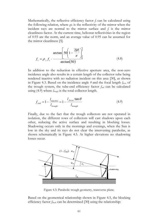
61

Mathematically, the reflective efficiency factor fr can be calculated using the following relation, where ρ┴ is the reflectivity of the mirror when the incident rays are normal to the mirror surface and fc is the mirror cleanliness factor. At the current time, heliostat reflectivities in the region of 0.93 are the norm, and an average value of 0.95 can be assumed for the mirror cleanliness [5].

50arctan

2150arctan

cr ff (4.8)

In addition to the reduction in effective aperture area, the non-zero incidence angle also results in a certain length of the collector tube being rendered inactive with no radiation incident on this area [30], as shown in Figure 4.3. Based on the incidence angle θ and the focal length lfocus of the trough system, the tube-end efficiency factor fend can be calculated using (4.9) where ltrough is the total collector length.

trough

focus

trough

inactive

endl

l

l

lf

tan11 (4.9)

Finally, due to the fact that the trough collectors are not operated in isolation, the different rows of collectors will cast shadows upon each other, reducing the active surface and resulting in blocking losses. Shadowing occurs only in the mornings and evenings, when the Sun is low in the sky and its rays do not clear the intervening parabolas, as shown schematically in Figure 4.5. At higher elevations no shadowing losses occur.

Figure 4.5: Parabolic trough geometry, transverse plane.

Based on the geometrical relationship shown in Figure 4.5, the blocking efficiency factor fblock can be determined [30] using the relationship:

62

cos

cos z

tr

sp

blockw

lf limited between 0 and 1 (4.10)

where lsp is the separation distance between adjacent rows of troughs, wtr the width of the trough collector, θz the solar zenith angle (4.4) and θ the trough incidence angle.

4 . 2 . 2 V a c u u m T u b e R e c e i v e r s

In order to be able to determine the outlet temperature and mass flow that can be obtained from the receiver for a given set of operating conditions, it is necessary to develop a mathematical model of the heat and mass transfer that takes place within the absorber.

The most common absorber for parabolic trough collection systems consists of a metal tube surround by a glass envelope within which a vacuum is maintained [30]. This is shown schematically in Figure 4.6. The metal tube is coated with a selective coating, which reduces the emissivity, limiting the heat losses.

Figure 4.6: Vacuum tube absorber for parabolic trough collectors.

In order to model the behaviour of the absorber, three partial differential equations can be elaborated, giving the temperature profiles for the heat transfer fluid f, absorber tube t and glass envelope e. Energy balances can be performed on the solid and fluid phases present, as well as the glass envelope, using the following hypotheses:

Heat and mass transfer phenomena are purely axial

The module perimeter is impermeable (no loss of mass)

No axial conduction within the fluid

The partial different equations are linked by heat flux terms, resulting from heat transfer between the different components of the system. The incident solar flux is absorbed by the solid absorber which then transfers this heat by convection to the liquid being drawn through the tube. The absorber loses heat by convection and radiation to the envelope, with

63

also loses heat to the environment by the same mechanisms. For the heat transfer liquid, the energy balance leads to the following differential equation:

fttitf

ff

fb TTPx

TcM

t

TcA

(4.11)

where αtf is the heat transfer coefficient between the absorber tube and the fluid, calculated using (4.13). Af is the flow area, M the mass flow through the tube, Pti the internal perimeter of the tube. All fluid properties are evaluated at bulk temperature. The increase in temperature of the heat transfer liquid can be seen to result entirely from convective exchange with the solid phase. In addition to the equation above, the boundary condition at the inlet can be defined:

tTtxT inf ,0 (4.12)

where Tin is the fluid inlet temperature. The heat transfer between the tube and the fluid can be calculated using the Dittus-Boelter equation [12] for fully turbulent flow:

33.08.0PrRe023.0Nu D

f

ittf

dk

d

(4.13)

where dit is the internal tube diameter, ReD the diameter-based Reynolds number and Pr the Prandtl number. All fluid properties are evaluated at bulk temperature. For the absorber tube, the energy balance leads to the following differential equation:

tftitft

ttt

ttt TTPx

TAk

t

TAc

2

2

´qTTU etete (4.14)

where At is the cross-sectional area of the tube, Ute the linear heat transfer rate (in W/mK) between the solid tube and the glass envelope, Pti and Pte are the internal and external perimeters of the tube respectively, τe the transmittance of the glass envelope and q˝ the local heat source (in W/m2) resulting from the absorption of solar radiation (§4.2.1). The following boundary condition can be written for the extremities of the tube:

64

tetesftitf

Lx

t

tt TTUTTPdx

dTAk

,0

´qe (4.15)

The heat transfer between the tube and envelope results from a combination of natural convection and radiation and the overall linear heat transfer rate is thus the sum of convection and radiation terms:

radncte UUU (4.16)

Assuming that the vacuum within the envelope is imperfect, and thus some air remains [30], the natural convection term can be determined based an expression proposed by Raithby and Holland [12], which gives:

otie

eff

ncdd

kU

ln2 (4.17)

where an effective heat conductively keff is used instead of the molecular heat conductivity of the air and die and dot are the internal diameter of the envelope and the outer diameter of the tube respectively. The effective heat conductivity is given [12] by the correlation:

4

1

Pr861.0

Pr386.0

air

eff

k

k x …

4

1

3

5

5

3

5

3

3

4

3

ln2

ieot

otie

air

pb

et

rr

rr

k

cgTT

(4.18)

where kair is the thermal conductivity of air, g the gravitational acceleration, β the thermal expansion coefficient, υ the kinematic viscosity and rie and rot are the internal radius of the envelope and the outer radius of the tube respectively. All fluid properties are evaluated at the annulus temperature, given by the mean temperature of the tube and the envelope. A vacuum pressure of 7 kPa can be assumed within the envelope [30]. The heat transfer rate by radiation between long concentric cylinders can be determined based on their respective emissivities and the view factor [12] between the exchanging surfaces:

65

ot

ie

e

e

t

eteteirad

d

d

TTTTPU

11

22

(4.19)

where σ is the Stefan-Boltzmann constant and εt and εe are the emissivities of the tube and envelope respectively. The tube is usually coated with a low-emissivity coating, the emissivity of which increases with the temperature of the surface. SANDIA [16] provides a linear function for the emissivity:

06597.0000327.0,05.0max tt T (4.20)

The evolution of the tube emissivity is shown in Figure 4.7. The emissivity of the glass envelope can be considered to have a value of 0.9.

Figure 4.7: Absorber tube emissivity as a function of temperature.

For the envelope, the energy balance leads to the following differential equation:

ettee

eee

eee TTUx

TAk

t

TAc

2

2

´1 qTTP eeaeeea (4.21)

where Ae is the cross-sectional area of the tube, αea the heat transfer coefficient between the glass envelope and its surroundings, Pee the external perimeter of the glass envelope and Ta the ambient temperature. The following boundary condition can be written for the extremities of the tube:

etteeaeeea

Lx

t

tt TTUTTPdx

dTA

,0

(4.22)

66

The heat transfer between the envelope and the environment results from a combination of natural convection and radiation; the overall heat transfer coefficient is thus the sum of natural convection and radiation terms:

radncea (4.23)

For a long horizontal cylinder, Churchill and Chu [12] propose the following correlation for the natural convection heat transfer coefficient:

air

oencd

k

dNu

2

3

6

1

27

8

16

9

Pr559.01

387.06.0

oe

air

pa

ae dk

cgTT

(4.24)

where doe is the outer diameter of the glass envelope.

The radiation heat transfer coefficient can be calculated using:

22

aeaeerad TTTT (4.25)

The frictional pressure drop ΔPf created by flow through the piping can be determined using the standard pressure drop formula:

2

2u

d

LfP b

it

t (4.26)

where f is the friction factor, dit the internal diameter of the pipe, Lt the length of the collector, ρb the bulk density of the fluid and u its flow velocity. The friction factor can be determined [1] using the analytical Churchill formula (4.27) where ReD is the diameter-based Reynolds number and A is a dimensionless factor that takes into account the effects of the specific tube roughness ks:

Given the complexity and number of equations involved, no analytical solution exists for the temperature and pressure profiles within the absorber. However, using numerical methods, a solution can be obtained with a finite-difference approach.

67

12

1

2

3

16

16

12

Re

37530

1

Re

88

D

D

A

(4.27)

p

s

D d

kA

27.0Re

7

1ln457.2

9.0 (4.28)

4 . 3 T w o - T a n k M o l t e n S a l t S t o r a g e

In order to determine the outlet temperatures available from the storage tanks, a mathematical model for the heat and mass transfer within the unit is required. Energy balances can be performed on the two-tank system, using the following hypotheses:

Uniform liquid temperature within tanks

Uniform air temperature within tanks

Heat transfer occurs between air, liquid, the environment and the ground

Schematically, the two tank storage system can be represented as shown in Figure 4.8. The empty dimensions of the tanks are given by the height ho and diameter do. Both tanks are capable of holding the entire salt volume in case of emergencies [34], during which the entire contents would be transferred from one tank to the other.

Within the hot tank, an energy balance gives the differential equation (4.29) for the temperature Tht of the storage medium where ρs is the salt density, cs its specific heat, At the tank cross-sectional area, hht the current height of liquid within the tank and Qloss the rate of heat loss from the liquid. The inlet temperature of the salt supplied to the storage unit is Tin.

Heat exchange between the salt and the air contained within the tank depends on the internal heat transfer coefficient αint. The variation in height is governed by the mass balance within the tank (4.30) where Min and Mout are the inlet and outlet mass flows respectively.

68

Figure 4.8: Schematic layout of a two-tank storage system.

htins

in

ht

ht

httss TTcMdt

dThAc

ht

lossahhtt QTTA int (4.29)

out

ht

in

ht

ht

t MMdt

dhA (4.30)

The internal heat transfer between the liquid and the air is governed by natural convection. For the upper surface of a hot medium, Incropera [12] recommends this modified form of the McAdams correlation:

25.0

3int

6454.0

4Nu

o

aa

apa

ahht

a

oL d

k

cgTT

k

d

(4.31)

where k is the thermal conductivity, g the gravitational acceleration, β the thermal expansion coefficient, υ the kinematic viscosity cp the isobaric specific heat and the subscript a refers to the air.

The rate of heat loss from the liquid in the tank is given by a combination of losses through the external insulation, and losses to the ground:

ghtgrdtahtexthto

ht

loss TTATThPQ (4.32)

where Po is the perimeter of the tank, αext the heat transfer coefficient for heat loss through the external insulation, Ta the ambient temperature, αgrd the heat transfer coefficient to the ground and Tg the ground temperature, which can be considered constant [19] and equal to the annual average air temperature. Assuming a constant thickness of the

69

insulating material, the heat loss coefficient αext can be determined using the relation for conduction through a cylindrical section:

ncins

o

ins

o

ext k

d

ed

1

2

21ln

1

(4.33)

where kins is the conductivity of the insulating material, eins the thickness of the insulating layer and αnc the natural convection coefficient. Assuming that the ground can be considered as a semi-infinite conducting medium [19], the heat loss coefficient αgrd can be determined using the shape factor [12] formulation:

grd

o

ins

ins

grd k

d

k

e

8

1

(4.34)

where kgrd is the thermal conductivity of the ground.

A second energy balance gives the following differential equations for the temperature Tah of the trapped hot air:

ahap

in

ah

ah

htotpa TTcMdt

dThhAc

ah

losshtaht QTTA int (4.35)

where ρa is the air density, cp its isobaric specific heat, hht the current height of storage liquid within the tank, ho the empty height of the tank and Ta the ambient temperature. Heat exchange between the salt and the air depends on the internal heat transfer coefficient αint which can be determined using (4.31). The mass flow of air Mah into the tank can be determined based on the mass flow of salt:

in

ht

out

ht

in

ht

out

ht

in

ht

out

ht

s

a

in

ah

MM

MMMMM

0

(4.36)

The rate of heat loss from the air in the tank is given by the combination of losses through the external insulation, and losses through the roof:

70

aah

ins

ins

texthtoo

ah

loss TTe

AhhPQ

(4.37)

where Po is the perimeter of the tank and the external heat loss coefficient αext can be calculated using (4.33).

An identical set of equations can be elaborated for the both the hot and cold tanks; the key difference will be the thickness of the insulation layer and the inlet temperature of the salt. Given the complexity and number of equations involved, the evolution of the temperatures in both tanks is calculated using a finite difference technique.

4 . 4 R e h e a t S t e a m G e n e r a t o r

In order to be able to determine the mass flow, temperature and pressure of the steam fed to the turbine units, a model of the steam generator unit has been established. The Andasol 1 power plant under study is based on a reheat power block [25], and the corresponding layout of the steam generator is shown schematically in Figure 4.9.

Figure 4.9: Layout of the steam generators for Andasol 1

Modelling of the steam generator is based on a combination of effectiveness-NTU methods for determining the heat exchange effectiveness and pinch-point analysis for the calculation of the mass-flows of live steam produced. Simulation proceeds through three stages:

1. The heat exchange area and nominal pressure drop are calculated using the effectiveness-NTU method to design the

71

heat exchanger and select its geometry (number of tubes, spacing, etc.) based on a technique proposed by Staine [28].

2. During operation the off-design heat transfer coefficients can be calculated based on standard correlations [12], along with the new, off-design, NTU values and used to determine the off-design effectiveness of the heat exchangers.

3. Based on the transient inlet temperatures and minimum approach temperatures calculated from the heat exchanger effectiveness, pinch analysis techniques can be used to determine the mass-flows during off-design operation.

4 . 4 . 1 T h e E f f e c t i v e n e s s - N T U D e s i g n M e t h o d

Based on the nominal inlet temperatures for each stream, as well as on the nominal mass flow rates, the heat load and thus the required surface area for the heat exchangers can be calculated using effectiveness-NTU relations [12]. To determine the effectiveness of a heat exchanger, it is first necessary to define the maximum possible heat transfer rate between the two fluids, which would be achieved for a counter-flow heat exchanger of infinite area:

cs

in

hs

in TTCQ minmax (4.38)

where hs references the hot stream, cs the cold stream and Cmin is the smaller heat capacity rate (in W/K) of either the hot or cold stream. The actual heat transfer rate will be less than this, and it is therefore possible to introduce the efficiency ε of the heat exchanger, defined as the ratio between the actual heat exchanged and the maximum possible heat exchange. The actual heat exchange is therefore given by:

cs

in

hs

in TTCQQ minmax (4.39)

In this way, for a heat exchanger of given efficiency, the total heat load can be determined once the inlet conditions of the two streams are known. For any heat exchanger it can be shown [12] that the efficiency is a function of the ratio of the heat capacity rates Cr and a dimensionless parameter known as the number of transfer units (NTU):

rCf ,NTU (4.40)

with min

NTUC

UA and

max

min

C

CCr (4.41)

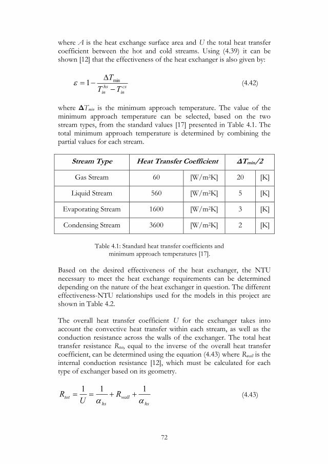
72

where A is the heat exchange surface area and U the total heat transfer coefficient between the hot and cold streams. Using (4.39) it can be shown [12] that the effectiveness of the heat exchanger is also given by:

cs

in

hs

in TT

T

min1 (4.42)

where ΔTmin is the minimum approach temperature. The value of the minimum approach temperature can be selected, based on the two stream types, from the standard values [17] presented in Table 4.1. The total minimum approach temperature is determined by combining the partial values for each stream.

Stream Type Heat Transfer Coefficient ΔTmin/2

Gas Stream 60 [W/m2K] 20 [K]

Liquid Stream 560 [W/m2K] 5 [K]

Evaporating Stream 1600 [W/m2K] 3 [K]

Condensing Stream 3600 [W/m2K] 2 [K]

Table 4.1: Standard heat transfer coefficients and minimum approach temperatures [17].

Based on the desired effectiveness of the heat exchanger, the NTU necessary to meet the heat exchange requirements can be determined depending on the nature of the heat exchanger in question. The different effectiveness-NTU relationships used for the models in this project are shown in Table 4.2.

The overall heat transfer coefficient U for the exchanger takes into account the convective heat transfer within each stream, as well as the conduction resistance across the walls of the exchanger. The total heat transfer resistance Rtot, equal to the inverse of the overall heat transfer coefficient, can be determined using the equation (4.43) where Rwall is the internal conduction resistance [12], which must be calculated for each type of exchanger based on its geometry.

hs

wall

hs

tot RU

R

111 (4.43)

73

Exchanger Type ε-NTU Relationship Condition

Counterflow

1

1ln

1

1NTU

rr CC

Cr < 1

1NTU

Cr = 1

Cross-flow

r

r

CC

1ln1

1lnNTU

Cr ≠ 0

Evaporator

Condenser 1lnNTU

Cr = 0

Table 4.2: Effectiveness-NTU relationships for various heat exchangers

The two α-values, for the hot stream and cold stream heat transfer coefficients, are selected again from standard values [18] presented in Table 4.1 based on the nature of the stream in question. Once the overall heat transfer coefficient is known, the required surface area for the exchangers can be determined by inverting relation (4.41).

U

CA minNTU (4.44)

where Cmin is the smaller of the two heat capacity rates for the exchanger streams [12]. The geometry of the exchanger must then be selected into order to ensure the desired flow conditions, and, most crucially, the desired heat transfer coefficients.

Standard heat transfer correlations ([12], [31]) can be used to calculate the flow speeds required within the exchanger to generate the heat transfer coefficients selected from Table 4.1. The two flow speeds obtained, one for the cold-stream flow ucs and one for the hot-stream flow uhs, can be used, along with the mass flow rates and fluid properties, to determine the flow areas and other geometrical features.

4 . 4 . 2 O f f - D e s i g n P e r f o r m a n c e

During off-design operation, the inverse technique to that described in §4.4.1 is used to calculate the heat load of the heat exchangers. Based on the fixed surface area calculated during the design phase, the NTU-value

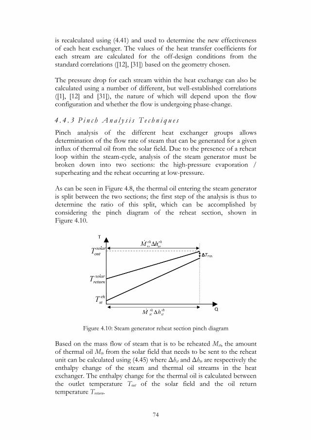
74

is recalculated using (4.41) and used to determine the new effectiveness of each heat exchanger. The values of the heat transfer coefficients for each stream are calculated for the off-design conditions from the standard correlations ([12], [31]) based on the geometry chosen.

The pressure drop for each stream within the heat exchange can also be calculated using a number of different, but well-established correlations ([1], [12] and [31]), the nature of which will depend upon the flow configuration and whether the flow is undergoing phase-change.

4 . 4 . 3 P i n c h A n a l y s i s T e c h n i q u e s

Pinch analysis of the different heat exchanger groups allows determination of the flow rate of steam that can be generated for a given influx of thermal oil from the solar field. Due to the presence of a reheat loop within the steam-cycle, analysis of the steam generator must be broken down into two sections: the high-pressure evaporation / superheating and the reheat occurring at low-pressure.

As can be seen in Figure 4.8, the thermal oil entering the steam generator is split between the two sections; the first step of the analysis is thus to determine the ratio of this split, which can be accomplished by considering the pinch diagram of the reheat section, shown in Figure 4.10.

Figure 4.10: Steam generator reheat section pinch diagram

Based on the mass flow of steam that is to be reheated Mst, the amount of thermal oil Mto from the solar field that needs to be sent to the reheat unit can be calculated using (4.45) where Δhst and Δhto are respectively the enthalpy change of the steam and thermal oil streams in the heat exchanger. The enthalpy change for the thermal oil is calculated between the outlet temperature Tout of the solar field and the oil return temperature Treturn.

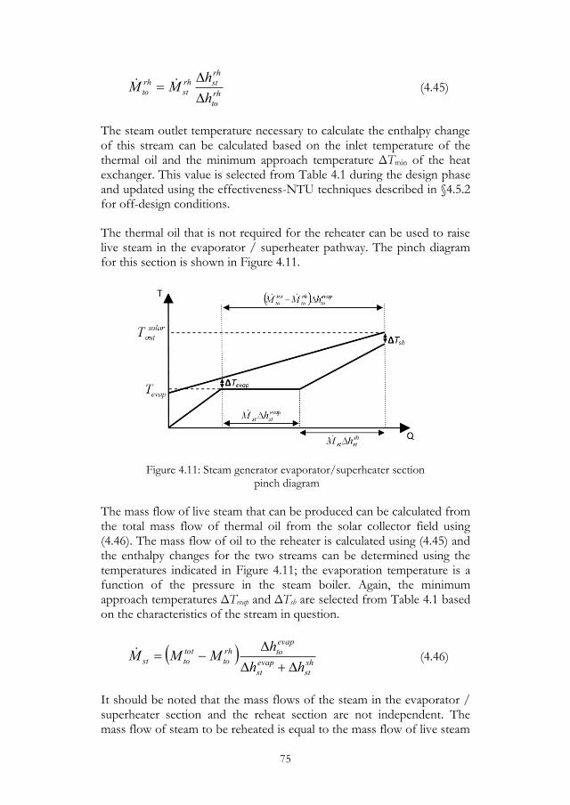
75

rh

to

rh

strh

st

rh

toh

hMM

(4.45)

The steam outlet temperature necessary to calculate the enthalpy change of this stream can be calculated based on the inlet temperature of the thermal oil and the minimum approach temperature ΔTmin of the heat exchanger. This value is selected from Table 4.1 during the design phase and updated using the effectiveness-NTU techniques described in §4.5.2 for off-design conditions.

The thermal oil that is not required for the reheater can be used to raise live steam in the evaporator / superheater pathway. The pinch diagram for this section is shown in Figure 4.11.

Figure 4.11: Steam generator evaporator/superheater section pinch diagram

The mass flow of live steam that can be produced can be calculated from the total mass flow of thermal oil from the solar collector field using (4.46). The mass flow of oil to the reheater is calculated using (4.45) and the enthalpy changes for the two streams can be determined using the temperatures indicated in Figure 4.11; the evaporation temperature is a function of the pressure in the steam boiler. Again, the minimum approach temperatures ΔTevap and ΔTsh are selected from Table 4.1 based on the characteristics of the stream in question.

sh

st

evap

st

evap

torh

to

tot

tosthh

hMMM

(4.46)

It should be noted that the mass flows of the steam in the evaporator / superheater section and the reheat section are not independent. The mass flow of steam to be reheated is equal to the mass flow of live steam

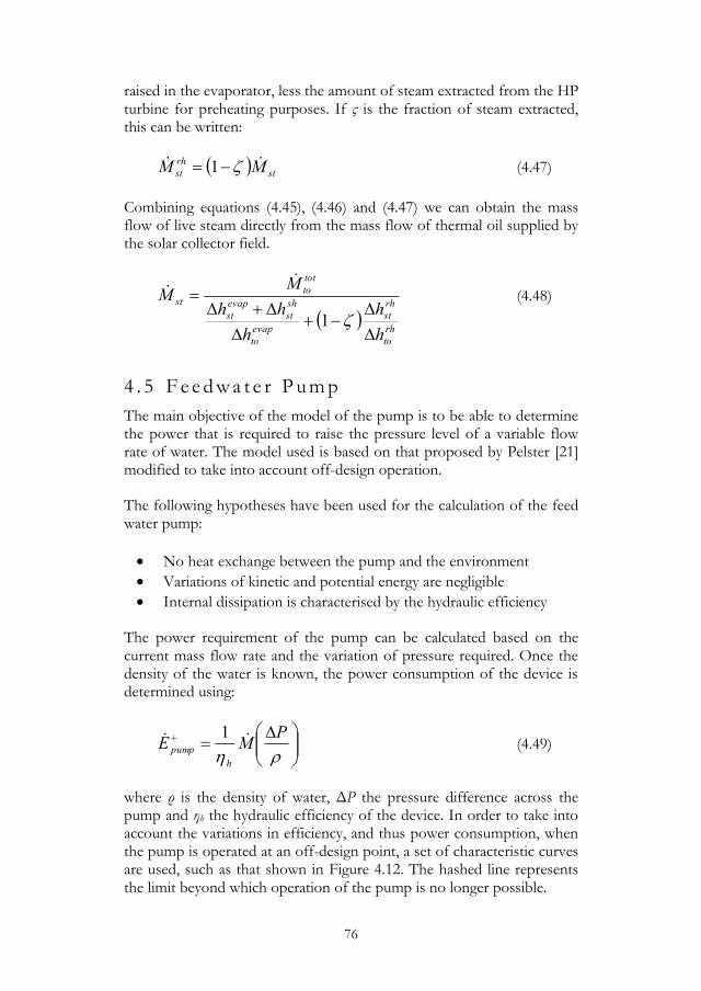
76

raised in the evaporator, less the amount of steam extracted from the HP turbine for preheating purposes. If ς is the fraction of steam extracted, this can be written:

st

rh

st MM 1 (4.47)

Combining equations (4.45), (4.46) and (4.47) we can obtain the mass flow of live steam directly from the mass flow of thermal oil supplied by the solar collector field.

rh

to

rh

st

evap

to

sh

st

evap

st

tot

to

st

h

h

h

hh

MM

1

(4.48)

4 . 5 F e e d w a t e r P u m p

The main objective of the model of the pump is to be able to determine the power that is required to raise the pressure level of a variable flow rate of water. The model used is based on that proposed by Pelster [21] modified to take into account off-design operation.

The following hypotheses have been used for the calculation of the feed water pump:

No heat exchange between the pump and the environment

Variations of kinetic and potential energy are negligible

Internal dissipation is characterised by the hydraulic efficiency

The power requirement of the pump can be calculated based on the current mass flow rate and the variation of pressure required. Once the density of the water is known, the power consumption of the device is determined using:

PME

h

pump 1

(4.49)

where ρ is the density of water, ΔP the pressure difference across the pump and ηh the hydraulic efficiency of the device. In order to take into account the variations in efficiency, and thus power consumption, when the pump is operated at an off-design point, a set of characteristic curves are used, such as that shown in Figure 4.12. The hashed line represents the limit beyond which operation of the pump is no longer possible.

77

Figure 4.12: Pump characteristic curves [10]

Although slight, the heating of the water as it passes through the pump must also be taken into account. This heating effect is due to dissipation of energy within the unit, and is therefore directly linked to the hydraulic efficiency. If the inlet water temperature is known, the outlet temperature can be calculated using the relation:

c

PT

cM

ETT

h

h

in

pumph

inout

11

(4.50)

where c is the specific heat capacity of the water.

78

79

5 Power Plant Performance Improvement

One of the key advantages of solar thermal power systems when compared with their closest rival, solar photovoltaics, is that through the inclusion of thermal energy storage and co-firing their capacity factor can be several times higher [22]. In particular, the inclusion of thermal storage allows the production of electricity to be decoupled from the instantaneously available solar flux: production can be continued during solar transients (i.e the passage of clouds) and into the evening after sunset, increasing availability and flexibility.

Despite the inclusion of storage tanks, state-of-the-art solar thermal power plants are not capable of operating around the clock. Co-firing with fossil- or bio-gas could provide an alternative to maintain operation once the storage tanks are empty; however, in Spain (where Andasol 1 is located) co-firing is limited by current legislation to a maximum of 15% energy input [25] on a yearly basis. Supplementary firing can thus be used to cope with solar transients or extend the operating time, but is insufficient to prevent regular interruption of electricity production.

Figure 5.1: Thermal power flow and turbine loads for a day with intermittent solar irradiation.

80

It is this starting and stopping of the plant that provides the opportunity for increased electricity production due to faster starts. As is shown in Figure 5.1, a significant increase in turbine output is possible when shifting from a cold to a hot start. Given the large number of starts and stops that will occur throughout the year, this gain is multiplied many times over, giving rise to a significant potential for improvement.

5 . 1 S t e a m T u r b i n e M o d i f i c a t i o n s

The speed at which the steam-turbines can start is a function of the metal temperature within the units before start-up begins. This relationship is shown in Figure 5.2, for two sets of start-up curves given by the turbine manufacturers. As was explained in §1, these curves are established to limit the maximum thermal stresses experienced by the turbine units.

Figure 5.2: Turbine start-up time as a function of metal temperature

A number of proposed modifications to the turbine units have been evaluated, each of which could potentially maintain the metal temperature during idle periods and thus reduce start-up time. In this study, three modifications are considered:

1. Installation of additional insulation material, reducing heat losses from the casing to the atmosphere.

2. Installation of electrically-powered heat blankets, which provide heat to the external surface of the turbine casing underneath the insulation layer.

3. Increasing the temperature of the gland steam provided by the external supply during idle periods, providing heat to the interior of both the turbine casing and rotor at the location of the labyrinth joints.

81

5 . 1 . 1 I n s t a l l a t i o n o f A d d i t i o n a l I n s u l a t i o n

The simplest-seeming option for preventing the cool-down of the turbines is to increase the thickness of the insulating blankets placed around them, reducing heat losses to the atmosphere and allowing the internal temperature to be maintained for a longer time.

There are a number of limitations as to where external blankets can be placed on the turbines, preventing the entire turbine being sheathed in insulation. These limitations arise from assembly and maintenance requirements, as well as the necessity to keep some components of the turbine (such as the bearings) below a certain temperature. The locations where additional insulation can be installed are shown for the LP turbine in Figure 5.3

Figure 5.3: Installation of additional insulation on the LP turbine

5 . 1 . 2 I n s t a l l a t i o n o f H e a t B l a n k e t s

A second option is the installation of active heating blankets on the outer surface of the turbine between the casing and the insulation, as shown schematically in Figure 5.4. These blankets are supplied with electrical power, resulting in external heating of the turbine casing while they are operating. This active means of maintaining the turbine temperatures requires an external source of power; in order for it to be viable the increase in electrical output from faster start-up must outweigh the consumption of the blankets during idle periods.

Figure 5.4: Position of the external heat blankets

It is not necessary, or indeed desirable, to heat the turbine units uniformly. Typically, it is necessary to maintain the inlet of the turbines

82

warmer than the exhaust sections. In order to accommodate this, the heat blankets can be divided into three sections, each of which can be supplied with a different power density, resulting in differential heating. Again, no heating is applied to the bearings, which must be kept cool.

5 . 1 . 3 I n c r e a s i n g G l a n d S t e a m T e m p e r a t u r e

The third and final option is to increase the temperature of the gland steam that is injected into the turbine during idle periods to prevent the infiltration of air into the steam circuit.

Figure 5.5: Location of the labyrinth joint temperatures

As was described in §3.3, the gland steam network provides two temperatures of steam for injection: a high-temperature ‘hot’ gland steam and a lower temperature ‘cool’ gland steam. During idle operation, both injections take place at pressures slightly above that of the atmosphere, in order to achieve the goal of preventing air infiltration. Gland steam is injected into the labyrinth joints of both turbine units at the locations shown in Figure 5.5.

If the temperature of the gland steam is above that of the surrounding metal, heat is transferred to the turbine unit, maintaining its internal temperature. Increasing the gland steam temperature is thus potentially a useful means of adding heat to otherwise inaccessible regions within the turbine units.

The magnitude of increase in temperature that can be tolerated is fixed by material limits within the turbine; additional thermal stresses within

83

the turbine created by increased gland steam temperature need to be kept within acceptable limits.

5 . 2 D a i l y I m p r o v e m e n t ( P a p e r 2 )

A first analysis of the three potential turbine improvements was presented in Paper 2, along with a detailed presentation and validation of the steam-turbine models. The performance of each modification was evaluated individually, followed by a consideration of a combination of the different modifications. The net increase in daily output was calculated for two different cool-down durations.

In order to obtain an objective comparison of the performance of the different steam-turbine modifications, a standard test case was established, comprising a cold turbine start, a typical operating period (in this case 8 hours) followed by a shutdown. The evolution of the steam-turbine inlet conditions for this standard case is shown in Figure 5.6.

The metal temperature of the turbine units at different times after shut-down was determined and compared between different modifications to analyse their effectiveness. The impact of each modification on the casing and rotor of the turbine units was quantified separately in order to examine the relative influence on the two components.

5 . 2 . 1 K e y R e s u l t s

Two different cool-down durations were analysed based on the test-case shown in Figure 5.6, namely a short cool-down of 10h and a longer cool-down of 24h. The increase in metal temperature registered at start-up resulting from application of the measures is shown in Figure 5.7, for different intensities of the measures described in §5.1.

It can be seen in Figure 5.7 that the addition of extra insulation has relatively little influence on the steam-turbine casing temperatures and none at all on the rotor temperatures. This is due to the limited zones to which additional insulation can be added and the existence of thermal loss pathways that by-pass the insulation (i.e convection to the bearing oil and gland steam).

Heat blankets can be seen to have a strong impact on the casing temperatures, but this improvement does not translate to the rotor. It is therefore not possible to obtain faster turbine starts from the application of heat blankets alone, as the rotor remains cold and would suffer high thermal stresses if a faster start-up was sought. Fortunately, increasing the gland steam temperature was shown to have a strong positive

84

influence on the rotor temperatures as well as a lesser influence on the casing temperatures.

Figure 5.6: Turbine modification test case

Figure 5.7: Impact of applying each of the three improvements to the steam-turbine. Influence on the casing and rotor temperatures shown separately for

both the high- and low-pressure turbines.

A combination of heat blankets and an increase in gland steam temperature would seem therefore to be a promising combination of modifications. The effect of the combined application of these two measures was studied. The temperature increase at the end of the cool-down is translated into increased electricity production through the curves presented in Figure 5.2. For this first study, the ‘old’ curves from this figure were used.

85

To obtain the net increase, the consumption of the different temperature maintaining modifications must be taken into consideration, using (5.1) where ΔEstart is the increased electricity output due to a faster start, Qblk the power supplied to the heat blankets, Mgst the mass flow rate of gland steam when the turbine is idle, Δhgst the increase in gland steam enthalpy and tc the duration of the cool-down before start-up. In order to simplify analysis of the two different modifications, electrical heating of the gland steam is assumed.

cgstgstblkstart thMQEE (5.1)

As in the analysis of the single modifications, two cool-down durations are considered (10h and 24h). The net increase in daily electricity is shown for both cases in Figure 5.8.

Figure 5.8: Increase in daily output resulting from the application of a combination of heat blankets and increased gland steam temperature

on the day following the cool-down period.

The thinner, diagonal, contours in Figure 5.8 are lines of equal energy consumption for the turbine modifications, whereas the thicker contours represent a step change in daily electricity output resulting from moving to a faster start-up time. The optimal points highlighted are those combinations of modifications that result in a change to a faster start-up curve with minimum energy consumption by the temperature maintaining modifications.

In both cases, daily gains in net electricity production of above 9% are predicted for certain combinations of the modifications, resulting from a change from a cold-start to a warm-start. This initial study would therefore appear to show a strong potential for increased electricity production through dispatchability increase.

86

5 . 3 A n n u a l I m p r o v e m e n t ( P a p e r 3 )

The initial study presented in Paper 2 considered the potential improvement in dispatchability for two specific cool-down durations, showing a strong potential. However, these two cool-down are not necessary representative of the true possibility that exists for dispatchability increase. Throughout the year, the turbines will undergo a wide range of start-ups and cool-downs, and Paper 3 takes this into account by analysing the annual performance improvement.

The system models presented in §4 are used to simulate a year’s worth of operation and determine the nature and frequency of the different types of start-up and shut-downs experienced by the steam-turbines. The key meteorological data used as input data to the simulations is shown in Figure 5.9 and Figure 5.10. Data is taken from the Meteonorm database as well as the Soda-IS solar radiation service.

The annual performance improvement for the power plant was compared under two different assumed operating strategies:

1. A free operating mode, in which the power plant is run whenever possible. In the morning, the plant begins production once the collector field reaches nominal output, at night, electricity production continues until the storage tanks are empty.

2. A limited operating mode, in which the power plant is run during hours of peak demand, between 7am and 11pm. In the morning, the output of the collector field is sent to the storage tanks before 7am, at night, electricity production continues until 11pm at the latest.

Figure 5.9: Ambient temperature for Andasol 1, 2005 sample

87

Figure 5.10: Solar irradiation map for Andasol 1, 2005 sample

In both operating modes, co-firing with natural-gas is assumed, up to a maximum of 3 hours in total [25] per day (12.5%). During daytime, if the storage tanks are unable to supply the power the generation cycle, co-firing is used to avoid a shut-down for up to an hour. Co-firing is not used to extend operation at night in either operating mode.

5 . 3 . 1 K e y R e s u l t s

The analysis of the annual performance improvement proceeded through three key stages:

1. A year’s worth of operation is simulated based on the meteorological data presented in Figure 5.9 and Figure 5.10, for both operating modes.

2. The distribution of the different cool-down durations experienced by the turbines is determined and compared; the results are shown in Figure 5.11 and Figure 5.12.

3. The different combinations of modifications are applied to the steam-turbines and the change in start-up times analysed. This change is converted to a net increase in electrical output using (5.1); the ‘new’ start-up curves in Figure 5.2 were used for this second study.

The distributions shown in Figure 5.11 and Figure 5.12 highlight the fact that a wide range of idle-periods is experienced in both operating modes; however, a clear difference in the distribution of cool-down times can be identified which will influence the effectiveness of the different temperature-maintaining modifications.

88

Figure 5.11: Annual distribution of turbine cool-down times

when the power plant is operated in limited mode.

Figure 5.12: Annual distribution of turbine cool-down times

when the power plant is operated in limited mode.

The change from ‘old’ to ‘new’ start-up curves (see Figure 5.2) was motived by the realisation on the behalf of the turbine manufacture that the initial curves were too conservative, imposing long start-up times on the turbines when it was not always necessary to do so. The redefinition of the curves results in a ‘free’ improvement in annual production, with a value of 2.4% predicted for the free operating mode and 6.4% for the limited operation mode.

Figure 5.13: Increase in annual output resulting from the application of a combination of heat blankets and increased gland steam temperature.

89

In additional to this ‘free’ improvement, the deployment of temperature maintaining modifications (again a combination of heat blankets and gland steam temperature increase was analysed here) results in a further increase of up to 2.2% in the free operating mode and up to 3.1% in the limited operating mode, as shown in Figure 5.13.

The annual gains predicted for the modifications are considerably lower than for the two single-day cool-down cases studied in Paper 2. This is due in large part to the change in the start-up curves supplied by the turbine manufacturer. It should be noted that the 2.2% and 3.1% increases predicted after modification of the turbine apply on top of the 2.4% and 6.4% gains resulting simply from the change in start-up curves, for a cumulative 4.6 and 9.5% increase for the free and limited operating modes respectively; this is of the same order of magnitude as predicted in Paper 2 for the single day.

90

91

6 Conclusions

The output from a solar thermal power plant is strongly dependent on the available solar flux, which varies due to both the predictable daily evolution of the Sun’s position as well as the more unpredictable variations in local weather conditions. In order to maintain an acceptable lifetime for the steam-turbine components, the duration of transient operation should be minimised. To improve the dispatchability of solar thermal power plants, it is also of interest to accelerate the start-up of the turbines in order to bring power rapidly onto the grid once a sufficient intensity of solar radiation becomes available.

The limiting factor in the start-up speed of a steam-turbine based solar thermal power plant is the thermal stress within the turbine units during start-up. If the turbines can be kept warm when operation ceases, the speed of the following start-up can be increased, improving dispatchability and allowing additional electricity production.

In this licentiate thesis, three modifications that maintain the internal temperature of the steam-turbine units during idle-periods were studied and found to have different effectiveness. A combination of external heating blankets and an increase in gland steam temperature was found to be the most effective, allowing significantly faster start-ups when installed and used with sufficient intensity.

On a yearly basis, increases in net electricity production of up to 3% are predicted when these two modifications are deployed, as well as a great improvement in the flexibility of operation. The magnitude of the production increase depends upon the operating scheme adopted, highlighting the importance of correct operation on the performance of solar thermal power systems, especially when the interplay between power production, energy storage and dispatchability is considered.

Maintaining the temperature of the steam-turbines during idle periods would seem to be a viable possibility for solar thermal power plant operators. Doing so not only reduces the thermal stresses experienced by the units, extending their life-span, but also allows an increase in electrical output of the plant by making the turbines able to respond more quickly to the availability of solar irradiation. Both these outcomes will serve to increase the economic viability of solar thermal power plants based on steam-turbine technology, making them a more attractive alternative for investors and thus accelerating the deployment of solar thermal power.

92

6 . 1 O u t l o o k

This licentiate thesis has been performed as part of an on-going research programme at KTH, looking at different aspects of turbomachinery operation in solar thermal power plants. This thesis does not represent the conclusion of the work, merely a step along the road. Work on steam-turbine optimisation will continue; there remain a number of unanswered questions.

The performance analysis in these studies has so far been purely from a thermodynamic (energetics) point of view. Cost analysis of the different turbine modifications is a logical next step: the costs of electricity production and consumption are not the same, which will impact on the effectiveness of the different modifications.

Optimisation of the deployment of the different modifications will be an important focus of future work. Different intensities of heating can be applied in different heat blanket zones and the two gland steam sources can be heated by different amounts. Better distribution of the heating could result in reduced consumption for a similar start-up improvement. Additionally, further innovative temperature maintaining modifications should also be studied.

It should be noted that in this study it has been assumed that the only limiting factor on power plant start-up speed is the steam-turbine. The steam generator is another component with significant thermal inertia which may impose limitations on the speed with which the plant can be brought up to full load.

All these issues (and more!) will be examined in future PhD work.

93

References

[1] François Avellan, “Turbomachines Hydrauliques, Pertes Energétiques”, EPFL Laboratoire de Machines Hydrauliques, Lausanne, 2007

[2] J. Birnbaum, J. Feldhoff, M. Fichtner et al., “Steam Temperature

Stability in a Direct Steam Generation Solar Power Plant”, Proceedings of the

SolarPACES Conference, 14th-18th September, Berlin, 2009

[3] J. Birnbaum, M. Jöcker, K. Link et al., “Simulation of the Dynamic

Behaviour of Steam Turbines with Modelica”, Proceedings of the

International Modelica Conference, 20th-22nd September, Como, 2009

[4] Lucien Borel, Daniel Favrat, “Thermodynamique et Energétique I, de

l’Energie à l’Exergie”, Presses Polytechniques et Universitaires

Romandes, Lausanne, 2004

[5] Francisco Collado, “Quick Evaluation of the Annual Heliostat Field Efficiency”, Solar Energy, Volume 82 (2008), p. 379-384

[6] David Cooke, “Modelling of Off-Design Multistage Turbine Pressures by Stodola’s Ellipse”, Energy Incorporated, Richmond, 1983

[7] Michel Deville, “Méthodes des Différences Finies”, EPFL Laboratoire d’Ingénierie Numérique, Lausanne, 2007

[8] John Duffie, William Beckman, “Solar Engineering of Thermal Processes”, Third Edition, John Wiley & Sons, New Jersey, 2006

[9] H. Emberger, E.Schmid, E. Gobrecht, “Fast Cycling Capability for New Plants and Upgrade Opportunities”, Proceedings of the POWERGEN Asia Conference, Singapore, 2005

[10] H.E. Gallus, “Turboverdichter und Pumpen, Auswahl, Betriebsverhalten und Anwendung”, Technische Hochschule Aachen, 2006

[11] David Howell, Carole Nakhle, “Out of the Energy Labyrinth: Uniting Energy and the Environment to Avert Catastrophe”, I.B. Tauris, 2007

[12] Frank Incropera, David De Witt, “Fundamentals of Heat and Mass Transfer”, Sixth Edition, John Wiley & Sons, New York, 2007

94

[13] Gerard Kosman, Andrzej Rusin, “The Influence of the Start-Ups and Cyclic Loads of Steam Turbines conducted according to European Standards on the Component’s Life”, Energy, Volume 26 (2001), p. 1083-1099

[14] Geoffrey Basil Leyland, “Multi-Objective Optimisation applied to Industrial Energy Problems”, PhD Thesis #2572, EPFL Laboratoire d’Energétique Industrielle, Lausanne, 2002

[15 ] John Lindström, Samuel Fällman, Mats Lyrander et al., “Requirements and Solutions for Steam Turbines in Concentrated Solar Power Plants”, Proceedings of the POWERGEN Renewable Energy Conference, 6th-8th March, Las Vegas, 2007

[16] F. Lippke, “Simulation of the Part-Load Behavior of a 30 MWe SEGS Plant”, SAND95-1293, SANDIA National Laboratories, Albuquerque, 1995

[17] François Maréchal, “Modélisation et Optimisation des Systèmes Energétiques Industriels”, EPFL Laboratoire d’Energétique Industrielle, Lausanne, 2003

[18] François Maréchal, “Process Integration Techniques for Improving the Energy Efficiency of Industrial Processes”, EPFL Laboratoire d’Energétique Industrielle, Lausanne, 2008

[19] Nicolas Morel, Edgard Gnansounou, “Énergétique du Bâtiment”,

EPFL Laboratoire d’Energie Solaire, Lausanne, 2009

[20] Jari Nyqvist, Detleft Haje, Kenny Kleinerman, “The Refinement of

Industrial Steam Turbines for Efficient Application in Solar Thermal Power

Plants”, Proceedings of the SolarPACES Conference, 21st-24th

September, Perpignan, 2010

[21] Stefan Pelster, “Environomic Modeling and Optimization of Advanced Combined Cycle Power Plants”, PhD Thesis #1791, EPFL Laboratoire d’Energétique Industrielle, Lausanne, 1998

[22] Cédric Philibert, “The Present and Future use of Solar Thermal Energy as

a Primary Source of Energy”, International Energy Agency, Paris, 2005

[23] R. Pitz-Paal, J. Dersch, B. Milow, “ECOSTAR: European

Concentrated Solar Thermal Road-Mapping”, Deutsches Zentrum für Luft-

und Raumfahrt, 2004

95

[24] Asok Ray, “Dynamic Modelling of Power Plant Turbines for Controller

Design”, Applied Mathematical Modelling, Volume 4 (1980), p. 109-113

[25] C. Richter (Editor), “Solar Power and Chemical Energy Systems, Annual

Report”, International Energy Agency, 2008

[26] Mark Sawley, “Numerical Flow Modelling: Simulation of Fluid and

Granular Flows”, EPFL Laboratoire d’Ingénierie Numérique,

Lausanne, 2007

[27] James Spelling, Daniel Favrat, Andrew Martin et al., “Thermo-

Economic Optimisation of Solar Tower Thermal Power Plants”, Proceedings of

the ECOS Conference, 14-17th June, Lausanne, 2010

[28] Frédéric Staine, “Intégration Energétique des Procédés Industriels Etendue aux Facteurs Exergétiques”, PhD Thesis #1318, EPFL Laboratoire d’Energétique Industrielle, Lausanne 1994

[29] William Stine, Michael Geyer, "Power from the Sun",

www.powerfromthesun.net, 2001 (Accessed 5th June 2010)

[30] Thorsten Stuetzle, “Automatic Control of the 30 MWe SEGS VI

Parabolic Trough Plant”, Master Thesis, University of Wisconsin,

Madison, 2002

[31] John Thome, “Engineering Data Book III”, Wolverine Tube Inc.,

Huntsville, 2008

[32] John Twidell, Tony Weir, “Renewable Energy Resources, Second Edition”, Taylor & Francis, New York, 2006

[33] K. Ummel, D. Wheeler, “Desert Power: the Economics of Solar Thermal Electricity for Europe, North Africa, and the Middle East”, Center for Global Development, 2008

[34] K. Wang, R. West, F. Kreith et al., “High-Temperature Sensible Heat Storage Options”, Solar Energy Research Institute, Golden, 1985

96

97

Appendix: Insulation Data

98

99

Appendix: Papers

1. T. Strand, J. Spelling, B. Laumert, T. Fransson, “On the Significance of Concentrated Solar Power R&D in Sweden”, Proceedings of the World Renewable Energy Congress, Linköping, May 2011

2. J. Spelling, M. Jöcker, A. Martin, “Thermal Modelling of a Solar Steam-Turbine with a focus on Start-Up Time Reduction”, GT2011-45686, Proceedings of the ASME Turbo Expo, Vancouver, June 2011

3. J. Spelling, M. Jöcker, A. Martin, “Annual Performance Improvement for Solar Steam-Turbines through the use of Temperature-Maintaining Modifications”, Solar Energy (Manuscript Submitted)

100