NBER WORKING PAPER SERIES

STATE DEPENDENCE AND ALTERNATIVE EXPLANATIONS FOR CONSUMERINERTIA

Jean-Pierre DubéGünter J. HitschPeter E. Rossi

Working Paper 14912http://www.nber.org/papers/w14912

NATIONAL BUREAU OF ECONOMIC RESEARCH1050 Massachusetts Avenue

Cambridge, MA 02138April 2009

We thank Wes Hutchinson, Ariel Pakes, and Peter Reiss for comments and suggestions. We acknowledgethe Kilts Center for Marketing at the Booth School of Business, University of Chicago for providingresearch funds. The first author was also supported by the Neubauer Family Faculty Fund, and thesecond author was also supported by the Beatrice Foods Co. Faculty Research Fund at the Booth Schoolof Business. The views expressed herein are those of the author(s) and do not necessarily reflect theviews of the National Bureau of Economic Research.

NBER working papers are circulated for discussion and comment purposes. They have not been peer-reviewed or been subject to the review by the NBER Board of Directors that accompanies officialNBER publications.

© 2009 by Jean-Pierre Dubé, Günter J. Hitsch, and Peter E. Rossi. All rights reserved. Short sectionsof text, not to exceed two paragraphs, may be quoted without explicit permission provided that fullcredit, including © notice, is given to the source.

State Dependence and Alternative Explanations for Consumer InertiaJean-Pierre Dubé, Günter J. Hitsch, and Peter E. RossiNBER Working Paper No. 14912April 2009JEL No. D12,L0,M31

ABSTRACT

For many consumer packaged goods products, researchers have documented a form of state dependencewhereby consumers become "loyal" to products they have consumed in the past. That is, consumersbehave as though there is a utility premium from continuing to purchase the same product as they havepurchased in the past or, equivalently, there is a psychological cost to switching products. However,it has not been established that this form of state dependence can be identified in the presence of consumerheterogeneity of an unknown form. Most importantly, before this inertia can be given a structural interpretationand used in policy experiments such as counterfactual pricing exercises,alternative explanations whichmight give rise to similar consumer behavior must be ruled out. We develop a flexible model of heterogeneitywhich can be given a semi-parametric interpretation and rule out alternative explanations for positivestate dependence such as autocorrelated choice errors, consumer search, or consumer learning.

Jean-Pierre DubéUniversity of ChicagoBooth School of Business5807 South Woodlawn AvenueChicago, IL 60637and NBERjdube@chicagobooth.edu

Günter J. HitschUniversity of ChicagoBooth School of Business5807 South Woodlawn AvenueChicago, IL 60637guenter.hitsch@ChicagoBooth.edu

Peter E. RossiUniversity of ChicagoBooth School of Business5807 South Woodlawn AvenueChicago, IL 60637peter.rossi@ChicagoBooth.edu

1 Introduction

Researchers in both economics and marketing have documented a form of persistence in con-

sumer choice data in which consumers have a higher probability of choosing products that

they have consumed in the recent past (see, for example, Keane (1997) and Seetharaman,

Ainslie, and Chintagunta (1999)). Typically, the data used to document these findings are

consumer panels recording purchases of branded products. Accordingly, we will term this

form of persistence, inertia in brand choice. Inertia is typically captured by a choice model

specification which includes lagged choice variables. A structural interpretation of this model

is that past purchases alter the utility derived from further consumption of the same goods or

that consumers face some sort of psychological switching costs in changing brands. To distin-

guish structural interpretations from purely statistical measures, we will term the structural

interpretation, state dependence in choice. The distinction between statistical and structural

interpretations of persistence in choice is important from the point of view of evaluating

optimal firm policies such as optimal pricing.

There are two parts to our investigation. We document that inertia in brand choice exists

and is not due to a mis-specified distribution of heterogeneity in preferences or autocorrelated

choice errors. We then consider if the observed inertia can be interpreted as a structural

model of state dependence or is simply proxying for costly search or learning.

A standard alternative explanation for state dependence is that choice model errors are

autocorrelated. Although this gives rise to inertial behavior in choice, the implications for

firm policy are quite di!erent. Firms facing consumers with auto-correlated errors have no

way to influence the degree to which consumers are “loyal” to their products, while under the

state dependent interpretation consumers can be induced to be loyal by price reductions and

other promotional activities. We implement tests to conclude that autocorrelated errors are

unlikely to be the source of observed inertia.

Another possible source of measured inertia could be mis-specification of the distribution

of consumer heterogeneity in brand preferences and price sensitivity. It is well known that it is

di"cult to distinguish between state dependence and heterogeneity. It is particularly di"cult

2

to do so if the entire set of taste parameters are consumer-specific. For example, there is no

compeling argument to assume that consumer di!erences are confined to brand intercepts.

The data requirements for separating hetergeneity from state dependence are formidable. Not

only must moderately long panels of consumers be recorded but there must be some form of

exogenous brand switching which allows for a shift in the loyalty “state.” Fortunately, panel

data on consumer packaged goods is captured in environments where there are frequent price

discounts. These price discounts induce brand switching and should induce state dependence.

The empirical literature on state dependence assumes a normal distribution of heterogene-

ity1. There is no particular reason to assume that distributions of taste parameters should

exhibit symmetric and unimodal distributions. In might be argued, for example, that the dis-

tribution of brand intercepts should be multi-modal, corresponding to di!erent relative brand

preferences for di!erent groups of consumers. In order to establish that state dependence find-

ings are robust to distributional assumptions, we implement a very flexible, semi-parametric

specification consisting of a mixture of multivariate normal distributions. While we argue

that our Bayesian methods provide extreme flexibility while retaining desirable smoothness

properties, we also consider a form of model-free evidence that our heterogeneity specification

is adequate.

It can be argued that persistence is not derived from state dependence but could be the

result a costly search process. With high search costs, consumers may be reluctant to pay

the search cost to sample other brands. We demonstrate that, while we can’t eliminate the

existence of search costs explanations, they do not seem to be the driving force behind the

measured state dependence. To draw these conclusions, we make use of the availability of local

store advertising which is determined exogeneous to individual consumer choice but changes

search costs.

Others have advanced the hypothesis (see for example, Osborne (2007) and Moshkin and

Shachar (2002)) that learning behavior could give rise to inertia in choices. A generic impli-

cation of learning models is that choice behavior will be non-stationary even when consumers

1See, for example, Keane (1997), Seetharaman, Ainslie, and Chintagunta (1999), and Osborne (2007).Shum (2004) uses discrete distribution of heterogeneity.

3

face a stationary store environment. As consumers obtain more experience with any set of

products, the amount of learning declines and their posterior beliefs on product quality con-

verge to a degenerate distribution. On the other hand, a state dependence model implies that

there will be a stationary distribution of consumer choice, given a stationary input process for

prices. We use this key feature to distinguish learning from state dependence and see little

evidence of learning.

Our goal is to document that state dependence survives a battery of tests and alternative

explanations and provide support for those who wish to interpret state dependence as a

structural model of utility. In a separate paper (Dubé, Hitsch, and Rossi (forthcoming)), we

explore the implications of models with inertia for equilibrium prices under the assumption

that the inertial terms can be given a structural interpretation.

2 Model and Econometric Specification

Our baseline model consists of households making discrete choices among J products in a cat-

egory and an outside option each time they go to the supermarket. The timing and incidence

of trips to the supermarket, indexed by t, are assumed to be exogenous. To capture inertia in

choices, we take the standard approach, often termed “state-dependent demand,” and assume

that current utilities are a!ected by the previous product chosen in the category. For ease of

exposition, we drop the household-specific index below. In the empirical specification, all the

model parameters will be household specific.

The utility index from product j at time period t is

ujt = !j + "pjt + #I {st = j} + $jt (2.1)

where pjt is the product price2 and $jt is the standard iid error term used in most choice

models. In the model given by (2.1), the brand intercepts represent a persistent form of vertical

2Other characteristics of the store environment facing the household could be entered into the “utility”model. But, then it may be problematic to interpret this as a utility specification. For example, manyresearchers include in-store advertising variables directly in the choice model. In Section 5, we consider asearch-theoretic interpretation of the role of displays.

4

product di!erentiation that captures a household’s intrinsic product (or brand) preferences.

st " {1, . . . , J} summarizes the history of past purchases from the perspective of impact on

current utility. If a household buys product k in period t # 1, then st = k. If the household

chooses the outside option, then the household’s state remains unchanged: st = st!1. Some

term st the “loyalty” state of the household. If st = j, the household is said to be “loyal”

to brand j. While the use of the last purchase as the summary of the past purchases is

very frequently used in empirical work, it is by no means the only possible specification. For

example, Seetharaman (2004) considers various distributed lags of past purchases.

If # > 0, then the model in (2.1) will generate a form of inertia. If a household switches to

brand k, the probability of a repeat purchase of brand k is higher than prior to this purchase.

One possible interpretation is that # results a form of psychological switching costs (see Farrell

and Klemperer (2006)).

2.1 Econometric Specification

At the household level (indexed by h), we specify a multinomial logit model with the outside

good expected utility set to zero.

Pr (j) =exp

!

!hj + "h

j Pricej + #hI {s = j}"

1 +#J

k=1exp

$

!hk + "h

kPricej + #hI {s = k}%

(2.2)

If we denote the vector of household parameters$

!h1 , . . . ,!h

J , "h, #h%

by %h, then hetero-

geneity of household types can be accommodated by assuming that the collection of&

%h'

are

drawn from a common distribution. In the empirical literature on state dependent demand,

a normal distribution is often assumed, %h $ N$

%̄, V!

%

. Frequently, further restrictions are

placed on V! such as a diagonal structure (see, for example, Osborne (2007)). Other authors

restrict the heterogeneity to only a subset of the % vector. The use of restricted normal models

is due, in part, to the limitations of existing methods for estimation of random coe"cient logit

models.

If normal models for heterogeneity are unable to capture the full distribution of hetero-

geneity, then there is the potential to create a spurious finding of interia or the importance of

5

state dependence. For example, consider the situation in which there is a bimodal distribution

of preferences for a particular brand. One mode corresponds to a sub-population of consumers

who find the brand relatively superior to other brands in the choice set, while the other mode

corresponds to consumers who find this brand relatively inferior. The normal approximation

to a bi-modal distribution would be symmetric and centered at zero. The normal would not

exhibit much in the way of di!erences in brand preferences (certainly not as much as the

bimodal distribution). When applied to data, the model with the normal distribution would

have a likelihood that puts mass on positive inertia parameter values in order to accomodate

the observation that some households persistently buy (do not buy) one of the brands.

Rather than restricting the distribution of parameters across households, we want to

allow for the possibility of non-normal and flexible distributions. This poses a challenging

econometric problem. Even if we were to observe the&

%h'

without error, we would be

faced with the problem of estimating a high dimensional distribution (in the applications

below, we estimate models with 5-10 dimensional distributions). In practice, we have only

imperfect information regarding household level parameters which adds to the econometric

challenge. Even with hundreds of households, we may only have limited information for any

one household given that there are typically not more than 50 observations per household.

This requires a method that does not overfit the data. One approach to the problem of

overfitting is to use proper prior distributions which create forms of smoothing and parameter

shrinkage.

Our approach is to specify a hierarchical prior with a mixture of normals as the first stage

prior (see, for example, section 5.2 of Rossi, Allenby, and McCulloch (2005)).The hierarchical

prior provides one convenient way of specifying an informative prior which avoids the problem

of overfitting even with a large number of normal components. The first stage is a mixture

of K multivariate normals and the second stage consists of priors on the parameters of the

mixture of normals.

p!

%h|&, {µk,!k}"

=K

(

k=1

&k'!

%h|µk,!k

"

(2.3)

&, {µk,!k} |b (2.4)

6

Here the notation ·|· indicates a conditional distribution and b represents the hyper-parameters

of the priors on the mixing probabilities and the parameters governing each mixture compo-

nent.

As is well-known, a mixture of normals models is very flexible and can accommodate

deviations from normality such as thick tails, skewness, and multi-modality. A priori, we might

expect that brand preference parameters (intercepts) might have a multi-modal distribution.

The modes might correspond to sub-groups of consumers who very much like, very much

dislike, or who are indi!erent to the brand. In addition, we might expect the distribution

of price coe"cients to be skewed left since consumers should behave in accordance with a

negative price coe"cient and there may be some extremely price sensitive consumers. At the

same time, we do not expect preference parameters to be independent. Thus, we are faced

with the task of fitting a multivariate mixture of normals.

A useful alternative representation of the model in (2.3) and (2.4) can be obtained by

introducing a latent set of variables which indicate which component each consumer is drawn

from.

%h|&, {µk,!k} $ '$

%h|µindh,!indh

%

indh $ MN (&)

&, {µk,!k} |b

(2.5)

indh is a multinomial variable with probability vector, &. This representation is precisely that

which would be used to simulate data from a mixture of normals, but it is also the same idea

used in the MCMC method for Bayesian inference in this model, as detailed in the appendix.

Viewed as a prior, (2.5) puts positive prior probability on mixtures with di!erent numbers of

components, including mixtures with a smaller number of components than K. For example,

consider a model that is specified with a large number of components, K = 10. A priori,

there is a positive probability that indh " {1, . . . , 5}. This is also possible a posteriori. This

property of the posterior is important for parsimony. A posteriori, it is possible that some

mixture components are “shut down” in the sense that they have very low probability and are

never visited during the navigation of the posterior.

7

While the mixture of normals model (2.3) is notoriously di"cult to fit via maximization

methods, Bayesian MCMC methods are well-suited to conducting inference to this problem.

The proper priors that form the second stage of the hierarchical model insure that the poles

and other singularities that plague a maximization approach are avoided. Rossi, Allenby,

and McCulloch (2005) define a special customized hybrid Metropolis MCMC algorithm for

this model which is automatically tuned to each of the household level likelihoods (see pp.

135-136). This is particularly important for application to consumer choice data as some

households will not be observed to choose from among all possible choice alternatives and a

household-level MLE will be undefined for these households. Standard hybrid MCMC meth-

ods for hierarchical logit models (see the excellent survey on MCMC methods by Chib (2001))

are simply infeasible for data that include incomplete purchase histories. The Appendix pro-

vides details of the MCMC algorithm and prior settings.

Our MCMC algorithm provides draws of the mixture probabilities as well as the normal

component parameters. Thus, each MCMC draw of the mixture parameters provides a draw

of the entire multivariate density of household parameters. We can average these densities to

provide a Bayes estimate of the household parameter density. We can also construct Bayesian

Highest Posterior Density (HPD) regions3 for any given density ordinate to gauge the level

of uncertainty in the estimation of the household distribution using the simulation draws.

That is, for any given ordinate, we can estimate the density of the distribution of either all

or a subset of the parameters. In particular, marginals distributions can be calculated by

exploiting the fact that the marginal distribution of a sub vector of a mixture of multivariate

normals is the same mixture of the appropriate marginals for each component. A single draw

of the original of the marginal density for the ith element of % can be constructed as follows:

pr!i

(t) =K

(

k=1

&rk'i (t|µ

rk,!

rk) (2.6)

'i (t|µk,!k) is the univariate marginal density for the ith component of the multivariate

3The Bayesian Highest Posterior Density region is the Bayesian analogue of the confidence interval. The95 percent HPD is an interval which has .95 probability under the posterior. We can compute estimates ofthe HPD by using quantiles from the MCMC draws.

8

normal distribution, ' (µk,!k).

Some might argue that you do not have a truly non-parametric method unless you can

claim that your procedure consistently recovers the true density of parameters in the pop-

ulation of all possible households. In the mixture of normals model, this requires that the

number of mixture components (K) increases with the sample size. Our approach is to fit

models with successively larger numbers of components and gauge the adequacy of the number

of components by examining the fitted density as well as the Bayes factor (see model selection

discussion below) associated with each number of components. What is important to note

is that our improved MCMC algorithm is capable of fitting models with a large number of

components at relatively low computational cost.

2.2 Posterior Model Probabilities

In order to establish that the inertia we observe in the data can be interpreted as a true

state dependent utility, we will compare a variety of di!erent specifications. Most of the

specifications we will consider will be heterogeneous in that a prior distribution or random

coe"cient specification will be assumed for all utility parameters. This poses a problem in

model comparison as we are comparing di!erent and heterogeneous models. As a simple

example, consider a model with and without the lagged choice term. This is not simply a

hypothesis about a given fixed dimensional parameter, H0 : #=0, but a hypothesis about a set

of household level parameters. The Bayesian solution to this problem is to compute posterior

model probabilities and compare models on this basis. A posterior model probability is

computed by integrating out the set of model parameters to form what is termed the marginal

likelihood of the data. Consider the computation of the posterior probability of model Mi:

p (Mi|D) =

)

p (D|",Mi) p ("|Mi) d" % p (Mi) (2.7)

where D denotes the observed data, " represents the set of model parameters, p (D|",M1)

is the likelihood of the data for M1, and p (Mi) is the prior probability of model i. The first

9

term in (2.7 ) is the marginal likelihood for Mi.

p (D|Mi) =

)

p (D|",Mi) p ("|Mi) d" (2.8)

The marginal likelihood can be computed by reusing the simulation draws for all model

parameters that are generated by the MCMC algorithm using the method of Newton and

Raftery (1994).

p̂ (D|Mi) =

*

1

R

R(

r=1

1

p (D|",Mi)

+

!1

(2.9)

p (D|",Mi) is the likelihood of the entire panel for model i. In order to minimize overflow

problems, we report the log of the trimmed Newton-Raftery MCMC estimate of the marginal

likelihood. Bayesian Model comparison can be done on the basis of the marginal likelihood

(assuming equal prior model probabilities).

Posterior model probabilities can be shown to have an automatic adjustment for the e!ec-

tive parameter dimension. That is, larger models do not automatically have higher marginal

likelihood as the dimension of the problem is one aspect of the prior that always matters.

While we do not use asymptotic approximations to the posterior model probabilities, the

asymptotic approximation to the marginal likelihood illustrates the implicit penalty for larger

models (see, for example, Rossi, McCulloch, and Allenby (1996)).

log (p (D|Mi)) & log!

p!

D|"̂MLE,Mi

""

#pi

2log (n) (2.10)

pi is the e!ective parameter size for Mi and n is the sample size. Thus, a model with the

same fit or likelihood value but a larger number of parameters will be “penalized” in marginal

likelihood terms. Choosing models on the basis of marginal likelihood can be shown to be

consistent in model selection in the sense that the true model will be selected with higher and

higher probability as the sample size becomes infinite.

10

3 Data

For our empirical analysis, we estimate the logit demand model described above using house-

hold panel data containing all purchase behavior for the refrigerated orange juice and the 16 oz

tub margarine categories. The panel data were collected by AC Nielsen for 2,100 households

in a large Midwestern city between 1993 and 1995. In each category, we focus only on those

households that purchase a brand at least twice during our sample period. Hence we use 355

households to estimate orange juice, and 429 households to estimate margarine demand.

Table 1 lists the products considered in each category as well as the purchase incidence,

product shares and average prices. We define the outside good in each category as follows. In

the refrigerated orange juice category, we define the outside good as any fresh or canned juice

product purchase other than the brands of orange juice considered. In the tub margarine

category, we define the outside good as any spreadable product i.e. jams, jellies, margarine,

butter, peanut butter etc). In Table 1, we see a no-purchase share of roughly 24%, in refrig-

erated juice, and 46% in tub margarine. We use this definition of the outside good to model

only those shopping trips where purchases in the product category are considered.

In our econometric specification, we will be careful to control for heterogeneity as flexibly

as possible to avoid confounding loyalty with unobserved heterogeneity. Even with these

controls in place, it is still important to ask which patterns in our consumer shopping panel

give rise to the identification of inertial or state dependent e!ects. The marginal purchase

probability is considerably smaller than the re-purchase probability for all products considered.

While this evidence is consistent with inertia, it could also be a reflection of heterogeneity in

consumer tastes for brands. The identification of inertia in our context relies on the frequent

temporary price changes typically observed in supermarket scanner data. If there is su"cient

price variation, we will observe consumers switching away from their preferred products. The

detection of state dependence relies on spells during which the consumer purchases these less-

preferred alternatives on successive visits, even after prices return to their “typical” levels.

We use the orange juice category to illustrate the source of identification of inertia or state

dependence in our data. First, we observe spells during which a household repeat-purchases

11

the same product. Conditional on a purchase, we observe 1889 such repeat-purchases out

of our total 3328 purchases in the category. Second, we observe numerous instances during

which a spell is initiated by a discount price. We classify each product’s weekly prices as either

“regular” or “discount,” where the latter implies a temporary price decrease of at least 5%.

Focusing on non-favorite products, i.e. products that are not the most frequently purchased

by a household, nearly 60% of the purchases are for products o!ering a temporary price

discount. We compare the repeat-purchase rate for spells initiated by a price discount (i.e.

a household repeat-buys a product that was on discount when they previously purchased it)

to the marginal probability of a purchase in Table 2. For all brands of Minute Maid orange

juice, the sample repurchase probability conditional on a purchase initiated by a discount is

.74, which exceeds the marginal purchase probability of .43. The same is true for Tropicana

brand products with the conditional repurchase probability of .83 compared to the marginal

purchase probability of .57. This is suggestive that observed high repurchase rates are not

simply the result of strong brand preferences but are caused by some sort of inertia.

Inertia or persistence in brand choices can be viewed as one possible source of dependence

in choices over time even for the same consumer. Another frequently cited source of non-zero

order purchase behavior is household inventory holdings (see, for example, Erdem, Imai, and

Keane (2003)). If households have some sort of storage technology, then they may amass

a household inventory either to reduce shopping costs (assuming there is a category-specific

fixed cost of shopping) or to exploit a sale or price discount of short duration. It should be

emphasized that household stock-piling has implications for the quantity of purchases as well

as the timing of purchases. Our state dependence formulation suggests that the specific brand

purchased on the last shopping trip should influence the current brand choice. A model of

stock-piling simply suggests that as the time between purchases increases the hazard rate of

purchase should increase. We neither use the quantity of purchase nor the timing of purchase

incidence in our analysis. Finally, we should note that the possibilities for household inventory

of the products (especially, refrigerated orange juice) appear to be limited. In our data, over

80 per cent of all purchases are for one unit of the product, suggesting that stock-piling is not

12

pervasive.

4 Inertia, Heterogeneity, and Robustness

Heterogeneity and State Dependence

It is well-known that state dependence and heterogeneity can be confounded (Heckman

(1981)). We have argued that frequent price discounts or sales provide a source of brand

switching that can identify inertia or state dependence in choices separately from hetero-

geneity in household preferences. However, it is an empirical question as to whether or not

inertia is an important force in our data. With a normal distribution of heterogeneity, a

number of authors have documented that positive state dependence or inertia is present in

CPG panel data (see, for example, Seetharaman, Ainslie, and Chintagunta (1999)). Frank

(1962) and Massy (1966) document state dependence at the panelist level using older diary

data. However, there is still the possibility that these results confirming inertia are not robust

to controls for heterogeneity using a flexible or non-parametric distribution of preferences.

Our approach is to fit models with and without an inertia term and with and without various

forms of heterogeneity. It is particularly convenient that our mixture of normals approach

nests the normal model in the literature.

Table 3 provides log marginal likelihood results that facilitate assessment of the statistical

importance of heterogeneity and inertia. All log marginal likelihoods are estimated using a

Newton-Raftery style estimator that has been trimmed of the top and bottom 1 per cent of

likelihood values as is recommended in the literature. We compare models without hetero-

geneity to a normal model (a one component mixture) and to five and ten mixture component

models.

As is often the case with consumer panel data (Allenby and Rossi (1999)), there is pro-

nounced heterogeneity. In a model with an inertia or state dependence term included, the

introduction of normal heterogeneity improves the model fit dramatically. The log marginal

likelihood improves by more 20 percent when normal heterogeneity is introduced. If two

13

models have equal prior probability, the di!erence in log marginal likelihood is related to the

ratio of posterior model probabilities:

log

,

p (M1|D)

p (M2|D)

-

= log (p (D|M1)) # log (p (D|M2)) (4.1)

Introduction of normal heterogeneity improves the log marginal likelihood by more than 100

points, such that the ratio of posterior probabilities is more than exp (100), providing over-

whelming evidence in favor of a model with heterogeneity in both product categories.

The normal model of heterogeneity does not appear to be adequate for our data as the

log marginal likelihood improves substantially (by at least 50 points) when a five component

mixture model is used. For example, for margarine products in a model with an inertia term,

moving from one to five normal components increases the log marginal likelihood from -5613

to -5550. Remember that the Bayesian approach automatically adjusts for e!ective parameter

size (see section 2.2) and the increase in log marginal density observed in Table 3 represents

a meaningful improvement in fit.

Figures 1-4 provide direct evidence on the importance of a flexible distribution of hetero-

geneity. Each figure plots the estimated marginal distribution of intercept, price, and inertia

or “state dependence” coe"cients from the five component mixture in blue (here we use the

posterior mean as the Bayes estimate of each density value. The yellow envelope enclosing the

five component marginal densities is a 90 percent pointwise HPD region. The one component

fitted density is drawn in red. A number of the parameters exhibit a dramatic departure from

normality. For example, the Shedd’s brand of margarine has a noticeably bimodal marginal

distribution across households. One mode is centered on a positive value (all intercepts should

be interpreted as relative to the “outside” good which is defined as other products in the cat-

egory) indicating strong brand preference for Shedd. The other mode is centered on a value

closer to zero, reflecting consumers who view Shedd’s as comparable to other products in

the category. One could argue that distributions with multiple modes are more likely to be

the norm rather than the exception with any set of branded products. The price coe"cient

(Figures 2 and 4) is also non-normal, exhibiting pronounced left skewness. Again, this might

14

be expected that there is a left tail of extremely price sensitive consumers. We note that the

prior distribution for the price coe"cient is symmetric and centered at zero.

Thus, there is good reason to doubt the appropriateness of the standard normal assumption

for many choice model parameters. This opens the possibility that the findings documenting

the importance of state dependence or inertia in choices are influenced, at least in part, by

arbitrary distributional assumptions. However, the importance of the inertia or “state depen-

dence” remains even when a flexible five component normal is specified. The log marginal

likelihood increases from -5575 to -5501 when inertia terms are added to a five component

model for margarine and from -4528 to -4434 in refrigerated orange juice. Figures 2 and 4

show that the marginal distribution of the inertia parameter is well approximated by a normal

distribution for these two product categories. While this is not definitive evidence, it does

suggest that the findings of inertia or state dependence in the literature are not artifacts of

the normality assumption commonly used.

The five component normal mixture is a very flexible model for the joint density of choice

model parameters. However, before we can make a more generic “semi-parametric” claim

that our results are not dependent on the form of the distribution, we must provide evidence

of the adequacy of the five component distributional model. Our approach to this is to fit

a ten component model. Many would consider this to be an absurdly highly parametrized

model. For the margarine category, the ten component model would have a “nominal” number

of 449 parameters (the coe"cient vector is 8 dimensional4). The log marginal likelihood

declines from five to ten components; from -5551 to -5559 for margarine and -4434 to -

4435 for orange juice. These results marginally favor the 5 component model over the 10

component, but, more importantly, indicate no value from increasing the model flexibility

beyond five components. We feel that the posterior model probability results in conjunction

with the high flexibility of the models under consideration justify the conclusion that we have

accommodated heterogeneity of an unknown form.

4There are 36 x 10 = 360 unique variance-covariance parameters plus 10 x 8 mean parameters plus 9mixture probabilites = 449.

15

Robustness Checks

State Dependence or a Mis-Specified Distribution of Heterogeneity? Some may

still doubt if we have indeed found inertia or if the lagged choice coe"cient simply proxies for

a mis-specification of the distribution of heterogeneity. We perform a simple check to test for

this possibility. Suppose there is no state dependence and that the coe"cient on the lagged

choice picks up taste di!erences across households that are not accounted for by the assumed

functional form of heterogeneity. Then, if we randomly reshu#e the order of shopping trips,

the coe"cient on the lagged choice will not change and still provide misleading evidence for

inertia. In Table 3 we show the log marginal likelihood for a five component model with an

inertia term, which we fitted to our data with randomly reshu#ed purchase sequences. The

log marginal likelihood for the randomized sequence data is approximately the same as for

the model without the inertia terms, and much lower than the log marginal density of the

model with properly ordered data and the inertia term. We thus find strong evidence against

the possibility that the lagged choice proxies for a mis-specified heterogeneity distribution.

State Dependence or Autocorrelation? While the randomized sequence test gives us

confidence that we have found convincing evidence of a non-zero order choice process, it

does not help distinguish between an inertia or state dependence model and a model with

auto-correlated choice errors. Using normal models and a di!erent estimation method, Keane

(1997) finds that state dependent and auto-correlated error models produce very similar re-

sults. However, the economic implications of the two models are markedly di!erent. With a

structural interpretation for inertia as a form of state dependent utility, firms can influence

the loyalty state of the customer and this has, for example, long-run pricing implications,

while the autocorrelated errors model does not allow for interventions to induce inertia or

loyalty to specific brands.

In order to distinguish between a model with a lagged choice or state dependent regressor

and a model with autocorrelated errors, we implement the suggestion of Chamberlain (1985).

We consider a model with a five component normal mixture for heterogeneity, no lagged

16

choice or state dependent term, but including the lagged prices defined as the prices at the

last purchase occasion. In a model with state dependence, price can influence the loyalty

(or state) variable and this will influence subsequent choices. In contrast, in a model with

auto correlated errors, it is not possible to influence persistence in choices using exogenous

variables. In Table 3, we compare the log marginal likelihood of the model without state

dependence and a five component normal mixture with the log marginal likelihood of the

same model including lagged prices. For margarine, the addition of lagged prices improves

the log marginal likelihood by more than 50 points and by more than 100 points for refrigerated

orange juice. This is strong evidence in favor of a “state dependence” specification with lagged

choices.

A limitation of the Chamberlain suggestion (as noted by both Chamberlain himself and

Erdem and Sun (2001)) is that consumer expectations regarding prices (and other right hand

side variables) might influence current choice decisions. Lagged prices might simply proxy for

expectations even though there is no state dependence at all. Thus, the importance of lagged

prices as measured by the log marginal likelihood is suggestive but not definitive.

As another comparison between a model with auto correlated errors and a state dependent

model, we exploit the price discounts or sales in our data. Since auto correlated errors are not

synchronized across households nor with price discounting by the retailer, we can di!erentiate

between state dependent and auto-correlated error models by examining the impact of price

discounts on measured state dependence. The intuition for this test is as follows. In a world

of serially correlated errors, households that are induced by price discounts to switch to a

new product will not exhibit inertia or persistence in choice. However, in a world with state

dependence, brand switching induced by any reason should create persistence. To implement

this idea, we interact the loyalty variable with an indicator for whether the loyalty state was

initiated by a discount or not (i.e. whether the last product purchased was purchased on

discount).

ujt = !j + "jpjt + #1I {st = j} + #2I {st = j} · I {discountst= j} + $jt (4.2)

17

The term, discountt, indicates whether the brand to which the consumer is currently loyal

was on discount when it was last purchased. In a model with auto-correlated errors, the

loyalty e!ect should dissipate for loyalty states generated by discounts, i.e. #1 + #2 = 0.

Table 3 provides a comparison of the log marginal likelihoods for the specification in (4.2);

the log marginal likelihood values for the discount interaction term are in the last row of the

table. The interaction term does improve model fit but by a modest 15-20 log density points.

It remains an open question as to whether measured state dependence changes materially

when we compare the distribution of the state dependence conditional on a past purchase

that was or was not on discount. Recall that we allow for an entire distribution of parameters

across the population of consumers so that we cannot provide the Bayesian analogue of a point

estimate and a confidence interval. Instead, we plot the fitted marginal distribution of #1 and

#1 +#2 in figure 5. The blue density curve is from our baseline model without any interaction

term (2.1), the red is the inertial or state dependence e!ect conditional on a discount on the

focal brand during the previous purchase occasion (labelled “lagged sale”) (denoted #1 in 4.2),

and the green is the e!ect conditional on no discount (labelled “no lagged sale”) (denoted

#1 + #2 in 4.2). There is little di!erence between the three densities for the orange juice

category and a slight shift toward zero with a lagged sale in the margarine category. We

conclude that there is scant evidence to support the claim that auto correlated errors are the

source of measured inertia.

Brand-Specific State Dependence

In the basic utility specification (2.1), the inertia e!ects are governed by one parameter that is

constrained to be the same across brands for the same household. There is no particular reason

to impose this constraint other than parsimony. Several authors have found the measurement

of inertial e!ects to be di"cult (see, for example, Keane (1997), Seetharaman, Ainslie, and

Chintagunta (1999), and Erdem and Sun (2001)) even with a one component normal model

for heterogeneity. The reason for imposing one “state dependence” or inertia parameter could

simply be a need for greater e"ciency in estimation. However, it would be misleading to

18

report state dependent e!ects if these are limited to, for example, only one brand in a set of

products. It also might be expected that some brands with unique packaging or trade-marks

might display greater inertia than others. It is also possible that the formulation of some

products may induce more inertia via some mild form of “addiction” in that some tastes are

more habit-forming than others. For these reasons, we consider an alternative formulation of

the state dependence model with brand-specific loyalty parameters. Our Bayesian methods

have a natural advantage for more highly parametrized models in the sense that if a model is

weakly identified from the data, the prior keeps the posterior well-defined and regular.

A five component mixture of normals with brand specific inertia fits the data with a

higher log marginal likelihood for both categories. For margarine, the log marginal likelihood

increases from -5551 to -5505 when brand specific e!ects are introduced into state dependence.

There is an even more dramatic increase for the orange juice products, from -4436 to -4364.

However, there is a di!erence between substantive and statistical significance. For this reason,

we plot the fitted marginal densities for the inertia or “state dependence” parameters for each

brand in figures 6 and 7. The distributions displayed in figure 6 compare the baseline model

with models that allow for di!erent inertia distributions for each brand. Interestingly, all

four distributions are centered close to the baseline, constrained specification. In the orange

juice category, figure 7 plots the distributions of inertia parameters for the four highest share

brands. In this category, the 96oz brands have higher inertia than the 64oz brands. We should

note that the prior distribution5 on the inertia parameters is centered at zero and very di!use.

This means that data has moved us to a posterior which is much tighter than the prior and

moved the center of mass away from zero. Thus, our results are not simply due to the prior

specification but are the result of evidence in our data.

The main conclusion is that allowing for brand-specific inertia does not reduce the impor-

tance of inertial e!ects nor restrict these e!ects to a small subset of brands.5It should be noted that, as detailed in the appendix, our “prior” is a prior on the parameters of the mixture

of normals – the mixing probabilities and each component mean vector and covariance matrix. This inducesa prior on the distribution over parameters and the resultant marginal densities. While this is of no knownanalytic form, the fact that our priors on each component parameters are di!use mean that the prior on thedistributions is also di!use.

19

5 Alternative Sources of Inertia: Search and Learning

We have established that inertial e!ects remain even with a very flexible distribution of

heterogeneity, are robust to mis-specification of heterogeneity and are unlikely to be the result

of auto correlated taste shocks. This holds out the possibility that changes in the exogenous

variables such as price can change the brands for which households exhibit inertia and, thus,

may have implications for firm policy. However, to evaluate these firm policy implications

requires a structural interpretation that the inertia term represents a form of state dependence

in which the utility for brands that have been recently purchased is altered. In this section, we

consider the role of consumer search and product learning as possible alternative explanations.

We assess the extent to which our findings of inertia in brand purchase might be explained,

not by state dependent utility, but by search or learning behavior. We do not postulate

specific structural models of search or learning which would involve some strong structural

assumptions on consumer behavior. Rather, we focus on aspects of consumer behavior that

di!erentiate search or learning explanations from state dependence and that can be directly

observed in our data.

Search

There can be no doubt that consumers face search costs in the recall of identities and location

of products in a store. Hoyer (1984) found that consumers spent, on average, only 13 seconds

“from the time they entered the aisle to complete their in-store decision.” Furthermore, only

11% of consumers examined 2 or more products before making a choice in a given product

category. Facing high search costs, consumers may purchase the products that they can easily

recall or locate in the store. These products are likely to be the products which the consumer

has purchased most recently. In this situation, consumers would display persistence or inertia

in product choice as they may not be willing to pay the implicit search costs for investigating

products other than those recently purchased.

In order to distinguish between inertia due to state dependence and inertia due to high

search costs, we exploit data on in-store advertising, sometimes termed “display” advertising.

20

Retailers frequently add signage and even rearrange the products in the aisle so as to call

attention to specific products. In the refrigerated orange juice category, 17.5% of the chosen

items had an in-store display during the shopping trip (in the margarine category displays are

seldom present)6. A display can be thought of as an intervention that reduces a consumer’s

search cost.

In the marketing literature, it is often assumed that consumers only choose among a subset

of products in any given category. This subset is called the consideration set. Mehta, Rajiv,

and Srinivasan (2003) construct a model for consideration set formation based on a fixed

sample size search process. Using data for ketchup and laundry detergent products, they find

that promotional activity, such as in-store displays, increase the likelihood that a product

enters a consideration set. This work a"rms the idea that in-store displays can reduce search

costs.

If displays a!ect demand via search costs, we should expect that a display increases the

probability of a purchase. In addition, if a consumer has purchased a specific product in the

past (st = j), then displays on other products should reduce the inertial e!ect or the tendency

for the consumer to continue to purchase product j. This can be implemented by adding a

specific interaction term to the baseline utility model:

ujt = !j +"pjt+#1I {st = j}+#2I {st '= j}·I {displayjt = 1}+(I {displayjt = 1}+$jt (5.1)

To illustrate the coding of the interaction term in (5.1), consider the case of two brands

and various display and inertia state conditions. If the consumer has purchased brand 1 in

the past (st = 1) and neither brand is on display, then utility for brand 1 relative to brand

2 is increased by #1. If brand 1 is on display, the utility di!erence increases by (. If brand

2 is also on display, the main e!ect of display, (, cancels out, but the interaction term turns

on with the potential to o!set the inertia e!ect. The di!erence between the utility for brand

1 and brand 2 due to state dependence and displays will be #1 # #2. Thus, #2 measures the

6There is a good deal of independent variation between displays and price discounts. No correlation betweenthe display dummy variable and the level of prices exceeds 0.4 in magnitude.

21

extent to which displays moderate the inertial e!ect of past purchases. If state dependence

entirely proxies for search costs and if search costs disappear in the presence of a display, then

we expect that #1 # #2 = 0.

Figure 8 plots the estimated marginal distribution of the inertia e!ect with and without

a display on alternative products. We can see that the two distributions are nearly identical.

There is virtually no evidence that displays a!ect persistence in choice. This leads us to

conclude that the measured state dependence is not merely a reduced-form e!ect that proxies

for in-store search costs.

The addition of a display main e!ect and interaction terms to the model improves the

model fit. The log marginal likelihood increases from -4434 to -4339 with the addition of the

display variables. However, most of this improvement in fit is due to the main e!ect terms

(-4434 to -4360). We interpret the finding that display has a main e!ect on the purchase

probability but does not change the measured degree of state dependence as evidence for

a direct utility-enhancing advertising e!ect of displays. Whatever the interpretation of the

main e!ect of displays, it is clear that that state dependence we estimate does not result from

search behavior.

Learning

It has often been argued that consumers have imperfect knowledge of the quality of products

and that the consumption of a product provides information about its true quality. This may

create persistence in choices over time. For example, suppose a consumer prefers brand B

to brand A under perfect information. However, initially the consumer has only imperfect

knowledge of the product’s quality, and expects that the utility from consuming A is larger

than the utility from consuming B. We then observe the consumer buying brand A until she

gains experience with brand B, for example if she tries B when the product is on promotion.

If learning is important in driving our state dependence findings, we would expect that

experienced consumers in the category would exhibit less inertia than inexperience consumers.

To proxy for shopping experience, we introduce a dummy for whether the primary shopper in

22

the household is over 35 years old. Let %h be the vector of household parameters (including

brand intercepts, price, and the inertia term). We then partition %h into a part associated

with the experienced shopper dummy and into residual unobserved heterogeneity that follows

the mixture of normals distribution:

%h = )zh + uh

uh $ N (µind,!ind) ; ind $ MN (&)(5.2)

) is a vector which allows the means of all model coe"cients to be altered by the experienced

shopped dummy, zh.

We find that the model fit is changed only slightly by the addition of the experienced

shopper dummy. The element of ) that allows for the possibility of shifting the distribution of

the inertia or state dependence coe"cient is imprecisely estimated with a HPD that covers 0.

For margarine, the posterior mean of this element is .17 with a 95 percent Bayesian credibility

region of (#.25, .60). For orange juice the mean is .12 with a 95 percent Bayesian credibility

region of (#1.9, 1.75). We conclude that there is no evidence that experienced shoppers exhibit

a di!erent distribution of the inertia coe"cient than less experienced shoppers.

A more powerful test of the learning hypothesis involves exploiting the fundamental dif-

ference between state dependence and learning models in terms of the implications for the

behavior of the choice process. Under state dependence, as long as the exogenous variables

(price, in our case) follow a stationary process, the choice process will also be stationary.

However, in any model where learning is achieved through purchase and consumption, the

choice process will be non-stationary. The consumers’ posterior distributions of product qual-

ity will tighten as more consumption experience is obtained and consumers will exhibit less

inertia. Eventually, consumers will behave in accordance with a standard choice model with

no parameter uncertainty.

We will exploit this di!erence in behavior to construct a comparison of state dependence

and learning model implications. Our panel is reasonably long and we might expect that

consumers will learn as they obtain more consumption experience with a brand. We define

23

brand level consumption experience as the cumulative number of purchases of the brand, Ejt.

We can interact the inertia or “state dependence” variable with this new experience variable

to provide a means of comparing the learning and pure state dependence models.

ujt = !j + "jpjt + #1I {st = j} + #2I {st = j} · Ejt + (Ejt + $jt (5.3)

Since the experience variable adds additional information to the choice model, we should

not directly compare the log marginal likelihood values of the interaction model (5.3) and the

baseline model (2.1). The hypothesis that state dependence proxies for learning has implica-

tions for the interaction term in equation (5.3). Under learning, the interaction term should

reduce state dependence as brand experience accumulates. Table 4 provides the likelihood

values for each category for a comparison of the model with the interaction term as in (5.3)

with a model containing only a main e!ect of brand experience:

ujt = !j + "jpjt + #1I {st = j} + (Ejt + $jt (5.4)

The marginal likelihood values increase by only 6 points when the interaction is added to (5.4)

in the margarine category. In the orange juice category, the addition of the interaction term

reduces the marginal likelihood. Figure 9 verifies that the interaction terms are centered at

0 and contribute little to the model. The red line in the figure plots the estimated marginal

distribution of #2 in (5.3), while the blue line plots the estimated marginal distribution of #1.

It might be argued that learning models only apply to products for which consumers

have little consumption experience. Substantial evidence for learning has been found for new

products by Ackerberg (2003), and Osborne (2007). Moshkin and Shachar (2002) find that

learning explains findings of state dependence for televisions programs, a product category

with a very large and frequent number of new products. In our case, the same products

have been in the market place for a considerable period of time. The households in the

data might be expected to show little evidence of learning given their experience with the

brands prior to their involvement in the panel. This underscores the importance of a flexible

24

model of heterogeneity. As a number of authors have noted, it is hard to distinguish learning

models with heterogeneous initial priors from a standard choice model with brand preference

heterogeneity. Indeed, Shin, Misra, and Horsky (2007) fit a learning model to a product

category populated by well-established products. Once they supplement their data with

survey data on household priors over product qualities, they measure very little learning.

6 The Dollar Value of State Dependence

The inclusion of the outside option in the model enables us to assign money-metric values to

our model parameters simply by re-scaling them by the price parameter (i.e. the marginal

utility of income), "# . The ratio represents the dollar equivalent of the utility premium in-

duced by state dependence. The state dependence demand model has the same implications

for consumer behavior as a model where consumers pay a specific amount of money when

switching products.7 Thus, the dollar equivalent ratio can be interpreted as a switching cost.

Table 5 displays selected quantiles from the distribution of the dollar state dependence

premium across the population of households. Some of the values on which this distribution

puts substantial mass are rather large values, others are small. To provide some sense of

the magnitudes of these values, we also compute the ratio of the dollar loyalty premium to

the average price of the products. For margarine products, the median dollar value of state

dependence is 28 per cent of the average product price; for orange juice, the ratio is slightly

lower at 21 per cent. However, there is a good deal of dispersion in the dollar value of state

dependence. At the 75th percentile of the dollar value distribution, the dollar value of state

dependence is 75 per cent of the purchase price for margarine and 41 per cent for orange juice.

These are large values and of the order of many examples of standard economic (as opposed

to psychologically derived) switching costs. For example, a cell phone termination penalty

of $150 might be much less than total cell phone expenditures over the expected length of

the contract. Another example of switching costs among packaged goods is razors and razor

blades; a consumer needs to purchase a new razor when switching the type of razor blades.

7See Dubé, Hitsch, and Rossi (forthcoming) for a detailed discussion.

25

Here the monetary switching cost is small relative to razor blade prices (?).

7 Conclusions

Inertia in consumer purchases has been documented in a variety of studies that use frequently

purchased consumer packaged goods. Typically, the lagged brand choice is found to influence

current brand choice positively and the results are interpreted as evidence in favor of state

dependent demand. It is well known, however, that state dependence can be confounded with

heterogeneity. Households that simply prefer one brand over the others in a product category

exhibit, what appears to be, persistence. In package goods panel data, there are frequent sales

which can induce brand switching and which can, in principle, di!erentiate state dependence

from heterogeneity.

Most empirical studies of state dependence use a normal distribution of heterogeneity.

There is good reason to believe that a normal distribution may be inadequate to capture

heterogeneity in many choice model parameters. It remains to be seen if the findings of state

dependence are robust to a more flexible heterogeneity distribution. We use a mixture of a

large number of multivariate normal distributions and exploit recent innovations in estimation

technology to implement a Bayesian MCMC procedure for this problem.

When applied to data on choices among brands of tub margarine and refrigerated orange

juice, we do, indeed, find very substantial evidence of non-normality. Findings of inertia in

brand choice are robust to a flexible distribution of preferences. It might be argued, however,

that our findings of inertia stem from auto-correlated choice error terms. As Keane (1997) has

pointed out, “state dependence” and auto-correlated error specifications can produce similar

patterns in the data. The key di!erence between state dependence and auto correlation is

that state dependence can be changed by external variables that alter the state and, therefore,

the pattern of persistence in the future. On the other hand, the persistence stemming from

auto-correlated errors cannot be altered. We exploit this di!erence between the models to

create a test for auto correlation based on whether the past purchase was initiated by a price

discount or not. We find evidence in favor of the state dependent model and against the

26

auto-correlated error specification.

The structural interpretation of the state dependence model is that, when a brand is

purchased, there is a utility premium accorded that brand in future choices. Equivalently, we

could interpret the state dependence model as a model of switching costs in which a cost is

paid (in utility terms) from switching to brands not bought on the last purchase occasion.

The switching cost interpretation of brand inertia or brand loyalty is based on the existence

of psychological switching costs rather than explicit monetary or product adoption costs.

Alternative structural models which could give rise to inertia in choices are models with

important brand search or learning e!ects. In search models, consumers may persist in pur-

chasing one brand if the costs of exploring other options are high. In learning models, what

appears to be inertia can arise because of imperfect information about product quality. Prod-

ucts which a consumer has consumed have less uncertainty in quality evaluation and this may

make consumers reluctant to switch to alternative products for which there is greater quality

uncertainty.

Comparison of the state dependent model to a model with learning or search e!ects could

be done conditional on a specific implementation of the search or learning model. Learning

models, for example, make explicit and restrictive distributional assumption regarding the

likelihood of signal information and priors. Typically, a normal prior and likelihood are

assumed for tractability. This poses a problem for a clean comparison of state dependence

and learning as the comparison is between state dependence and a specific parametric learning

model. Our approach is to examine those empirical implications of search and learning models

which are di!erent than those of a state dependence model.

For search models, we exploit the fact that we have in-store advertising data which can

alter the cost of search. Our findings are that there is little evidence consistent with a generic

implication of search models for choice under a regime of reduced search costs. For learning

models, we use the non-stationary implications of the learning model for choice behavior. A

state dependent model implies a stationary choice process (controlling for exogenous vari-

ables) while the learning model implies lower persistence in choices as consumers acquire

27

more information about a particular brand. The evidence in the data is consistent with the

stationary state dependence framework.

We have established a firmer basis for the structural interpretation of the state dependent

choice model for demand. This model implies that variables under firm control, such as prices,

can influence the future choice behavior of consumers. This opens a number of possibilities for

work on firm policy. In the companion pieces, Dubé, Hitsch, Rossi, and Vitorino (2008) and

Dubé, Hitsch, and Rossi (forthcoming), we explore the implications of the estimates switching

costs for dynamic pricing under multi-product monopoly and dynamic oligopoly respectively.

28

References

Ackerberg, D. A. (2003): “Advertising, Learning, and Consumer Choice in Experience

Good Markets: An Empirical Examination,” International Economic Review, 44(3), 1007–

1040.

Allenby, G. M., and P. E. Rossi (1999): “Marketing Models of Consumer Heterogeneity,”

Journal of Econometrics, 89, 57–78.

Chamberlain, G. (1985): “Heterogeneity, Omitted Variable Bias, and Duration Depen-

dence,” in Longitudinal Analysis of Labor Market Data, ed. by J. J. Heckman, and B. Singer,

chap. 1, pp. 3–38. Cambridge University Press.

Chib, S. (2001): “Markov Chain Monte Carlo Methods: Computation and Inference,” in

Handbook of Econometrics, ed. by J. J. Heckman, and E. Leamer, vol. 5, chap. 57, pp.

3570–3642. Elsevier Science B.V.

Dubé, J.-P., G. Hitsch, and P. E. Rossi (forthcoming): “Do Switching Costs Make

Markets Less Competitive?,” Journal of Marketing Research.

Dubé, J.-P., G. Hitsch, P. E. Rossi, and M. A. Vitorino (2008): “Category Pricing

with State-Dependent Utility,” Marketing Science, 27(3), 417–429.

Erdem, T., S. Imai, and M. P. Keane (2003): “Brand and Quantity Choice Dynamics

Under Price Uncertainty,” Quantitative Marketing and Economics, 1, 5–64.

Erdem, T., and B. Sun (2001): “Testing for Choice Dynamics in Panel Data,” Journal of

Business and Economic Statistics, 19(2), 142–152.

Farrell, J., and P. Klemperer (2006): “Coordination and Lock-In: Competition with

Switching Costs and Network E!ects,” draft, Handbook of Industrial Organization III.

Frank, R. E. (1962): “Brand Choice as a Probability Process,” The Journal of Business,

35(1), 43–56.

29

Heckman, J. J. (1981): “the Incidental Parameters Problem and the Problem of Initial Con-

ditions in Estimating a Discrete Time-Discrete Data Stochastic Process and Some Monte

Carlo Evidence",” in Structural Analysis of Discrete Data with Econometric Applications,

ed. by C. Manski, and D. McFadden, chap. 4, pp. 179–195. MIT Press.

Hoyer, W. D. (1984): “An Examination of Consumer Decision Making for a Common Repeat

Purchase Product,” Journal of Consumer Research, 11(3), 822–829.

Keane, M. P. (1997): “Modeling Heterogeneity and State Dependence in Consumer Choice

Behavior,” Journal of Business and Economic Statistics, 15(3), 310–327.

Massy, W. F. (1966): “Order and Homogeneity of Family Specific Brand-Switching Pro-

cesses,” Journal of Marketing Research, 3(1), 48–54.

Mehta, N., S. Rajiv, and K. Srinivasan (2003): “Price Uncertainty and Consumer Search:

A Structural Model of Consideration Set Formation,” Marketing Science, 22(1), 58–84.

Moshkin, N. V., and R. Shachar (2002): “The Asymmetric Information Model of State

Dependence,” Marketing Science, 21(4), 435–454.

Newton, M. A., and A. E. Raftery (1994): “Approximate Bayesian Inference with the

Weighted Likelihood Bootstrap,” Journal of the Royal Statistical Society, Series B, 56(1),

3–48.

Osborne, M. (2007): “Consumer Learning, Switching Costs, and Heterogeneity: A Struc-

tural Examination,” Discussion paper, Economic Analysis Group, Department of Justice.

Rossi, P. E., G. M. Allenby, and R. E. McCulloch (2005): Bayesian Statistics and

Marketing. John Wiley & Sons.

Rossi, P. E., R. E. McCulloch, and G. M. Allenby (1996): “The Value of Purchase

History Data in Target Marketing,” Marketing Science, 15(4), 321–340.

Seetharaman, P. B. (2004): “Modeling Multiple Sources of State Dependence in Random

Utility Models: A Distriburted Lag Approach,” Marketing Science, 23(2), 263–271.

30

Seetharaman, P. B., A. Ainslie, and P. K. Chintagunta (1999): “Investigating House-

hold State Dependence E!ects across Categories,” Marketing Science, 36(4), 488–500.

Shin, S., S. Misra, and D. Horsky (2007): “Disentangling Preferences, Inertia, and Learn-

ing in Brand Choice Models,” Discussion paper, University of Rochester.

Shum, M. (2004): “Does Advertising Overcome Brand Loyalty? Evidence from the Breakfast-

Cereals Market,” Journal of Economics and Management Strategy, 13(2), 241–272.

31

Appendix: MCMC and Prior Settings

The MCMC method applied here is a hybrid method with a customized Metropolis chain

for the draw of the household level parameters coupled with a standard Gibbs sampler for a

mixture of normals conditional on the draws of household level parameters. That is, once the

collection of household parameters are drawn, the MCMC algorithm treats these as “data”

and conducts Bayesian inference for a mixture of normals. Thus, there are “two” stages in the

algorithm.

%h|yh,Xh, indh, µindh,!indh

h = 1, . . . ,H (7.1)

ind,&, {µk,!k} |" (7.2)

" is matrix consisting of H rows, each with the %h parameters for each household, yh is the

vector choice observations for household h, and Xh is the matrix of covariates. The first

stage of the MCMC in (7.1) is a set of H Metropolis algorithms tuned to each household

MNL likelihood. The tuning is done automatically without any “pre-sampling” of draws

and is done on the basis of a fractional likelihood that combines the household likelihood

fractionally with the pooled MNL likelihood (for further details, see Rossi, Allenby, and

McCulloch (2005), chapter 5). It should be noted that this tuning is just for the Metropolis

proposal distribution. This procedure avoids the problem of undefined likelihoods for tuning

purposes. The household likelihood used in the posterior computations is not altered.

The second stage (7.2) is a standard unconstrained Gibbs Sampler for a mixture of normals.

The “label-switching” problem for identification in mixture of normals is not present in our

application as we are interested in the posterior distribution of a quantity which is label-

invariant, i.e. the mixture of normal density itself. The priors used are:

& $ Dirichlet (a)

µk|!k $ N$

µ, a!1µ !k

%

!k $ IW (*, *I)

32

The prior hyperparameters were assessed to provide proper but di!use distributions. a =

(.5/K,K), amu = 1/16, * = dim (%h) + 3. The Dirichlet prior on & warrants further comment.

The Dirichlet distribution is conjugate to the multinomial.#

a can be interpreted as the

size of a prior sample of data for which the classification of %h “observations” is known. The

number of observations of each “type” or mixture component is given by the appropriate

element of a. Our prior says that each type is equally likely and that there is only a very

small amount of information in the prior equal to a sample “size” of .5. As the number of

normal components increases, we do not want to change how informative the prior is; this is

why we scale the elements of the a vector by K.

Our computer code for this model can be found in the contributed R package, bayesm,

available on the CRAN network of mirror sites (see function rhierMnlRwMixture).

33

Table 1: Description of the Data

Margarine

Product Average Price %TripsPromise 1.69 13.11Parkay 1.63 4.98Shedd’s 1.07 12.66ICBINB 1.55 23.51no-purchase (% trips) 45.73# households 429# trips per household 18.25# purchases per household 9.90

Refrigerated Orange Juice

Product Average Price % Trips64oz MM 2.21 11.1Premium 64oz MM 2.62 7.0096oz MM 3.41 14.7Premium 64oz TR 2.73 28.864oz TR 2.26 6.76Premium 96 oz TR 4.27 7.99no-purchase (% trips) 23.75# households 355# trips per household 12.3# purchases per household 9.37

34

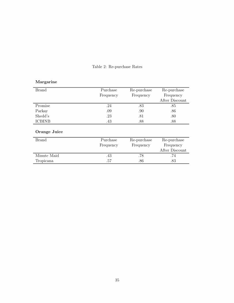
Table 2: Re-purchase Rates

Margarine

Brand PurchaseFrequency

Re-purchaseFrequency

Re-purchaseFrequency

After DiscountPromise .24 .83 .85Parkay .09 .90 .86Shedd’s .23 .81 .80ICBINB .43 .88 .88

Orange Juice

Brand PurchaseFrequency

Re-purchaseFrequency

Re-purchaseFrequency

After DiscountMinute Maid .43 .78 .74Tropicana .57 .86 .83

35

Table 3: Log Marginal Likelihood for State Dependence (SD) Specifications

Model Margarine Orange JuiceHomogeneous Model without SD -10755 -76125 Comp Normal without SD -5575 -45285 Comp Normal with lagged prices, no SD -5517 -4389Homogeneous Model with SD -8175 -62975 Comp Normal with SD -5501 -44345 Comp, SD, Randomized Purchase Sequence -5581 -45035 Comp, SD, Interaction with Discount -5537 -4419

36

Table 4: Learning and State Dependence

Model Margarine Orange Juice5-comp, SD -5551 -44345-comp, SD, experienced shopper dummy -5533 -44775-comp, SD, main e!ect of brand experience -5302 -42645-comp, SD, main and interaction e!ect of brand exp -5266 -4293

37

Table 5: Dollar Value of State Dependence

Margarine

Quantile Dollar Value Dollar Value/MeanPrice

10% $0.07 0.0425% $0.17 0.1150% $0.44 0.2875% $1.16 0.7590% $2.69 1.74

Orange Juice

Quantile Dollar Value Dollar Value/MeanPrice

10% $0.12 0.0425% $0.27 0.1050% $0.56 0.2175% $1.15 0.4290% $2.09 0.77

38

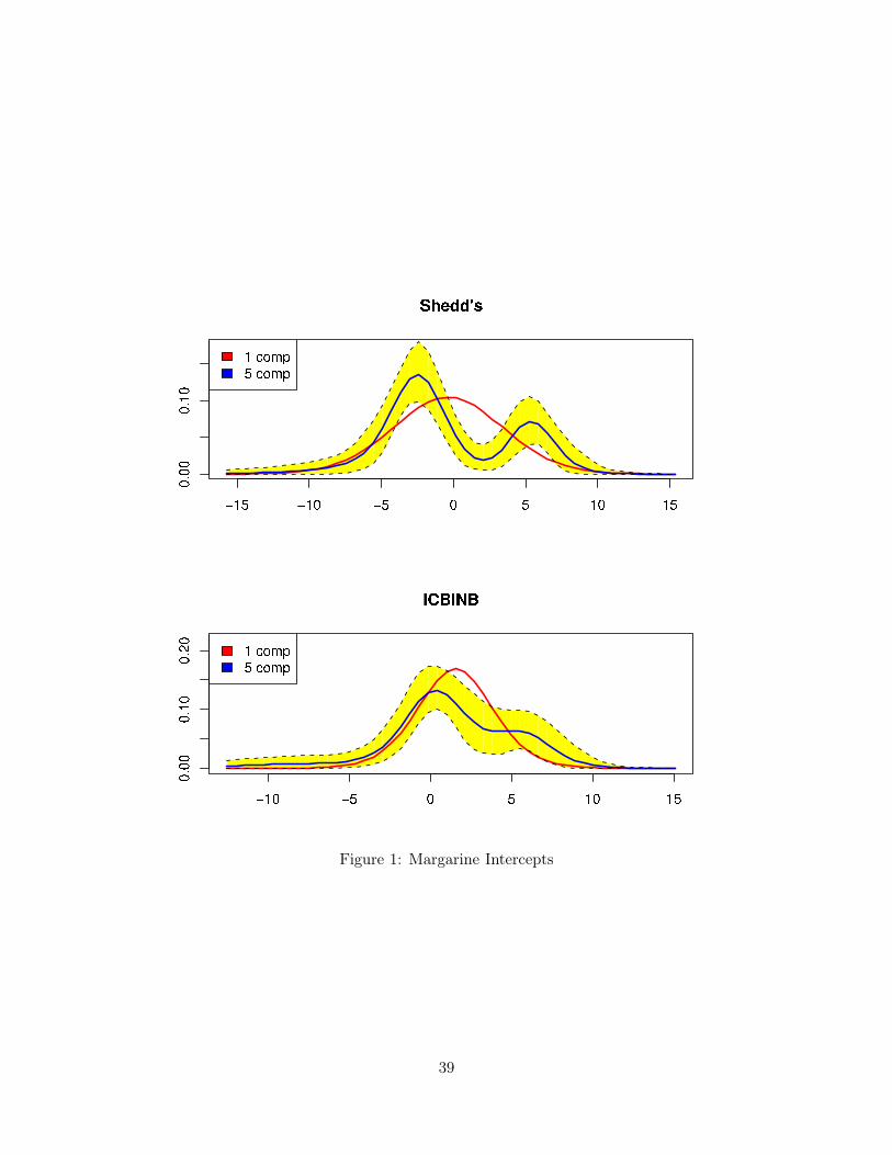
Figure 1: Margarine Intercepts

39

Figure 2: Price and State Dependence Coe"cients: Margarine

40

Figure 3: Refrigerated Orange Juice Brand Intercepts

41

Figure 4: Price and State Dependence Coe"cients for Refrigerated Orange Juice

42

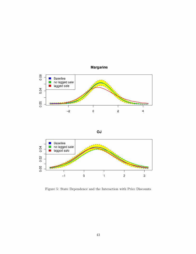
Figure 5: State Dependence and the Interaction with Price Discounts

43

Figure 6: Brand Specific State Dependence: Margarine

44

Figure 7: Brand Specific State Dependence: Orange Juice

45

Figure 8: Interaction Between State Dependence and Display

46

Figure 9: Interaction between State Dependence and Prior Brand Consumption

47