Collaborative Project

Holistic Benchmarking of Big Linked DataProject Number: 688227 Start Date of Project: 2015/12/01 Duration: 36 months

Deliverable 5.1.2Second Version of the Data StorageBenchmarkDissemination Level Public

Due Date of Deliverable Month 30, 31/05/2018

Actual Submission Date Month 30, 31/05/2018

Work Package WP5 - Benchmarks III: Storage and Curation

Task T5.1

Type Other

Approval Status Final

Version 1.0

Number of Pages 30

Abstract: This deliverable describes the development of the second version of the Data Storagebenchmark for HOBBIT. By introducing new features, such as the parallel execution of thebenchmark queries in a scenario based on real-world load, and the time compression ratioparameter, we were able to introduce an extended version of our benchmark for assessing BigLinked Data storage solutions for interactive applications.

The information in this document reflects only the author’s views and the European Commission is not liable for any use

that may be made of the information contained therein. The information in this document is provided "as is" without

guarantee or warranty of any kind, express or implied, including but not limited to the fitness of the information for a

particular purpose. The user thereof uses the information at his/ her sole risk and liability.

This project has received funding from the European Union’s Horizon 2020 research and innovation programmeunder grant agreement No 688227.

D5.1.2 - v. 1.0. . . . . . . . . . . . . . . . . . . . . . . . . . . . . . . . . . . . . . . . . . . . . . . . . . . . . . . . . . . . . . . . . . . . . . . . . . . . . . . . . . . . . . . . . . . . . . . . . . . .

History

Version Date Reason Revised by

0.1 11/05/2018 First draft Mirko Spasić, Milos Jovanovik

0.2 13/05/2018 Review Irini Fundulaki

1.0 25/05/2018 Final version Mirko Spasić, Milos Jovanovik

Author List

Organization Name Contact Information

OpenLink Mirko Spasić mspasic@openlinksw.com

OpenLink Milos Jovanovik mjovanovik@openlinksw.com

. . . . . . . . . . . . . . . . . . . . . . . . . . . . . . . . . . . . . . . . . . . . . . . . . . . . . . . . . . . . . . . . . . . . . . . . . . . . . . . . . . . . . . . . . . . . . . . . . . . .

Page 1

D5.1.2 - v. 1.0. . . . . . . . . . . . . . . . . . . . . . . . . . . . . . . . . . . . . . . . . . . . . . . . . . . . . . . . . . . . . . . . . . . . . . . . . . . . . . . . . . . . . . . . . . . . . . . . . . . .

Executive Summary

The demand for efficient RDF storage technologies has been steadily growing in recent years, dueto the increasing number of available Linked Data datasets and applications exploiting Linked Dataresources. With this, a growing number of applications require RDF storage solutions capable ofanswering SPARQL queries in interactive times, often over very large datasets. Given the number ofavailable RDF storage solutions, there is an need for objective means to compare technologies fromdifferent vendors. Consequently, there is a need for representative benchmarks that mimic the actualworkloads present in real-world applications. In addition to helping developers, such benchmarks aimto stimulate technological progress among competing systems and thereby accelerate the maturingprocess of Big Linked Data software tools.

One aspect in such benchmarking efforts is the benchmarking of data storage. As part of theHOBBIT project, we created the Data Storage benchmark, using the LDBC Social Network Benchmarkas a starting point. By introducing important modifications to its synthetic data generator and dataset,and by modifying and transforming its SQL queries to SPARQL, all while preserving the benchmark’smost relevant features, we were able to create the first version of the Data Storage benchmark forHOBBIT. Now, building on our previous work, we introduce new features and provide an extendednew version of the benchmark.

This deliverable outlines the details of how the second version of the Data Storage benchmarkfor HOBBIT was developed and tested. It focuses on the newly introduced parallel execution of thebenchmark queries, and the time compression ratio parameter, both of which enable storage evaluationbased on a real-world workload. The deliverables also describes the integration of the new version ofthe benchmark into the HOBBIT platform, and showcases the benchmark results of the baselineimplementation.

. . . . . . . . . . . . . . . . . . . . . . . . . . . . . . . . . . . . . . . . . . . . . . . . . . . . . . . . . . . . . . . . . . . . . . . . . . . . . . . . . . . . . . . . . . . . . . . . . . . .

Page 2

D5.1.2 - v. 1.0. . . . . . . . . . . . . . . . . . . . . . . . . . . . . . . . . . . . . . . . . . . . . . . . . . . . . . . . . . . . . . . . . . . . . . . . . . . . . . . . . . . . . . . . . . . . . . . . . . . .

Contents

1 Introduction 4

1.1 Requirements for the Data Storage Benchmark . . . . . . . . . . . . . . . . . . . . . . 4

2 Data Storage Benchmark Dataset 5

3 Data Storage Benchmark (DSB v2.0) 5

3.1 Key Performance Indicators . . . . . . . . . . . . . . . . . . . . . . . . . . . . . . . . . 7

4 Integration into the HOBBIT Platform 7

4.1 DSB Parameters . . . . . . . . . . . . . . . . . . . . . . . . . . . . . . . . . . . . . . . 7

4.2 Components . . . . . . . . . . . . . . . . . . . . . . . . . . . . . . . . . . . . . . . . . . 8

4.2.1 Benchmark Controller . . . . . . . . . . . . . . . . . . . . . . . . . . . . . . . . 9

4.2.2 Data Generator . . . . . . . . . . . . . . . . . . . . . . . . . . . . . . . . . . . . 9

4.2.3 Task Generator . . . . . . . . . . . . . . . . . . . . . . . . . . . . . . . . . . . . 10

4.2.4 System Adapter . . . . . . . . . . . . . . . . . . . . . . . . . . . . . . . . . . . . 11

4.2.5 Evaluation Module . . . . . . . . . . . . . . . . . . . . . . . . . . . . . . . . . . 11

4.2.6 Common API . . . . . . . . . . . . . . . . . . . . . . . . . . . . . . . . . . . . . 12

5 Evaluation 13

5.1 Sequential Tasks . . . . . . . . . . . . . . . . . . . . . . . . . . . . . . . . . . . . . . . 14

5.2 Parallel Tasks . . . . . . . . . . . . . . . . . . . . . . . . . . . . . . . . . . . . . . . . . 14

6 MOCHA Preliminary Challenge Results 18

References 20

A Tables 21

B Virtuoso Configuration 26

. . . . . . . . . . . . . . . . . . . . . . . . . . . . . . . . . . . . . . . . . . . . . . . . . . . . . . . . . . . . . . . . . . . . . . . . . . . . . . . . . . . . . . . . . . . . . . . . . . . .

Page 3

D5.1.2 - v. 1.0. . . . . . . . . . . . . . . . . . . . . . . . . . . . . . . . . . . . . . . . . . . . . . . . . . . . . . . . . . . . . . . . . . . . . . . . . . . . . . . . . . . . . . . . . . . . . . . . . . . .

1 Introduction

The demand for efficient RDF storage technologies has been steadily growing in recent years. Thisincrease is a result of the growing number of available Linked Data datasets and applications exploitingLinked Data resources. With this, a growing number of applications require RDF storage solutionscapable of answering SPARQL queries in interactive times, often over very large datasets. Given thenumber of available RDF storage solutions, there is an need for objective means to compare technologiesfrom different vendors. Consequently, there is a need for representative benchmarks that mimic theactual workloads present in real-world applications. In addition to helping developers, such benchmarksaim to stimulate technological progress among competing systems and thereby accelerate the maturingprocess of Big Linked Data software tools.

One aspect in such benchmarking efforts is the benchmarking of data storage. After a carefulconsideration of all available benchmarks and benchmark generation frameworks for querying LinkedData, we developed the first version of the Data Storage benchmark (DSB) for HOBBIT [6]. Thebenchmark is based on and extends the Social Network Benchmark (SNB), developed under the aus-pices of the Linked Data Benchmark Council (LDBC)1. LDBC introduced a new choke-point drivenmethodology for developing benchmark workloads, which combines user input with input from expertsystems architects [4]. Unlike other benchmarks which are specifically tied to a single technology [2, 7],SNB is much more generic, and can be used for the evaluation of pure graph database systems, sys-tems intended to manage Semantic Web data conforming to the RDF data model, distributed graphprocessing systems and traditional relational database systems that support recursive SQL.

In the first version of the Data Storage benchmark, we have created a benchmark based on the SNB-Interactive SQL version, along with a synthetic RDF dataset generator based on SNB’s DATAGEN,which was used in LDBC to generate a relational database. For the second version, we introduce parallelexecution of the benchmark queries, which simulates a real-world workload for the tested system. Wealso introduce a new parameter, time compression ratio, which allows an increase / decrease to thespeed of query issuing, i.e. modifies the speed of the social network activity simulation. This deliverableprovides a detailed description of these new features as part of the second version of the Data Storagebenchmark for HOBBIT. The deliverables also describes the integration of the new version into theHOBBIT platform, and showcases the benchmark results of the baseline implementation.

1.1 Requirements for the Data Storage Benchmark

The requirements that the Data Storage benchmark for HOBBIT has to meet, are:

• High insert rate with time-dependent and largely repetitive or cyclic data

• Possible exploitation of structure and physical organization adapted to the key dimensions of thedata

• Bulk load support

• Interactive complex read queries

• Simple lookups

• Concurrency1http://www.ldbcouncil.org/

. . . . . . . . . . . . . . . . . . . . . . . . . . . . . . . . . . . . . . . . . . . . . . . . . . . . . . . . . . . . . . . . . . . . . . . . . . . . . . . . . . . . . . . . . . . . . . . . . . . .

Page 4

D5.1.2 - v. 1.0. . . . . . . . . . . . . . . . . . . . . . . . . . . . . . . . . . . . . . . . . . . . . . . . . . . . . . . . . . . . . . . . . . . . . . . . . . . . . . . . . . . . . . . . . . . . . . . . . . . .

• High throughput

These requirements enable an efficient evaluation of data storage solutions which support interac-tive workloads in real-world scenarios, over various dataset sizes [1, 5].

2 Data Storage Benchmark Dataset

The second version of the Data Storage benchmark uses the same dataset as the first version. Thedataset is a synthetic RDF dataset, created by our data generator (DATAGEN). The DATAGEN wasbased on the Social Network Benchmark data generator, but was significantly modified and improvedfor the first version of DSB [6]. It generates synthetic RDF datasets which mimic an online socialnetwork and has real-world coherence. It can generate synthetic RDF datasets with a scale factor of1, 3, 10, 30, 100, etc. The number of triples per scale factor is shown in Table 1.

Table 1: Number of triples in the DSB datasets of different size.

SF # Triples

1 45.4M

3 136.5M

10 464.1M

30 1428.4M

100 4645.7M

The DSB DATAGEN is publicly available on GitHub2.

3 Data Storage Benchmark (DSB v2.0)

Our Data Storage Benchmark (DSB) is based on the LDBC Social Network Benchmark (SNB) andintroduces some important modifications related to the synthetic dataset and the benchmark queries.These changes, along with the choke points on which the queries are based, are described in extendeddetail in deliverable D5.1.1 [6], where the first version of DSB is presented. The improvements in-troduced in this version of the benchmark relate to the way the queries are executed, i.e. the queryworkload. In this second version of DSB, the query workload is more realistic, practical and pragmatic.

DSB v1.0 was single-threaded - at any point in the benchmark run there is only one running query,with the next one starting only after the previous one completes. With this approach, we examinedand appraised the best performance of the tested system for each query, by allowing the system tohave all resources available for the currently running query.

The KPIs collected using the first version of the benchmark are not useful for the deployment of asystem which would serve a social network. Primarily, the purpose of the benchmark is the comparison

2https://github.com/hobbit-project/DataStorageBenchmark-Dev

. . . . . . . . . . . . . . . . . . . . . . . . . . . . . . . . . . . . . . . . . . . . . . . . . . . . . . . . . . . . . . . . . . . . . . . . . . . . . . . . . . . . . . . . . . . . . . . . . . . .

Page 5

D5.1.2 - v. 1.0. . . . . . . . . . . . . . . . . . . . . . . . . . . . . . . . . . . . . . . . . . . . . . . . . . . . . . . . . . . . . . . . . . . . . . . . . . . . . . . . . . . . . . . . . . . . . . . . . . . .

of different triple stores, but also, in a real scenario, the benchmark should provide the relevant partieswith answers to the following question: is it possible to use a particular triple store (e.g. VirtuosoCommercial) as a storage component in the back-end of a social network application, if we have inmind the approximate number of users and available hardware resources? So, for that purpose, theaverage execution time of specific queries is not very relevant. Here, the throughput of concurrentqueries is much more important, and the ability of the system to provide the answers to the multiplequeries submitted at the same time, or almost at the same time, in reasonable and interactive times.This perspective served as a guideline for the second version of our benchmark.

The second version of DSB is multithreaded, allowing us to test the concurrency of the systemwith multiple queries running simultaneously. The majority of benchmarks test the parallel executionof multiple queries by simply having multiple query queues and running query-by-query per queue[3]. Our intent was not to just submit a large amount of queries at the same time, but to provide aworkload which mimics real-world activity in the social network domain, i.e. a workload which will bedriven by updates in the following sense.

Here, the updates represent social network events, such as adding a person to the social network,joining a group, posting a photo or a comment, liking a post, becoming the friend of a person, etc.All of these events, present in the real-world based synthetic dataset, have timestamps of when theyoccurred, so we can simulate a workload by using them. For instance, if there is a time delay betweentwo specific events of 10ms, the updates (as INSERT queries) corresponding to them will take place ina time span of 10ms. The workload, just like in SNB, is constructed by taking the updates (as INSERTqueries) from the dataset and mixing them with SELECT queries which have predefined frequencies(e.g. Query 1 should be performed once in every 132 update operation). The resulting query mix hastwo goals in mind [4]: to be somewhat realistic, and to be challenging for the query engine. For thefirst goal, the ratio between INSERT and SELECT queries is realistically determined (e.g. for each500 reads there is 1 write in Facebook’s database [8]). For the second goal, the idea is to make sureeach query type takes approximately equal amount of CPU time (i.e. queries that touch more data runless frequently) to avoid the workload being dominated by a single query [4]. This way, the workloadwill mimic the real-world usage of the data store serving the social network application.

This kind of workload will provide us with an answer to the following question: is the system undertest capable of serving a social network of the specific size? However, this does not seem enough totest the scalability of the system and the system behavior in a more demanding workload. How can westress it further? Having in mind the graph characteristics of the dataset, the most common approachhere is to provide a larger dataset, a dataset with more triples, i.e. a social network with more userswhere there are more updates per unit of time [4]. This is obvious because more users provide moreposts, comments and activity in general, represented as updates, or more precisely SPARQL INSERTqueries. They are bundled with SELECT queries by specified ratio, giving us more SPARQL SELECTqueries, as well. So, the benchmark scales well with increasing size of the dataset.

Is it possible to have more demanding workload, while keeping the size of the dataset unmodified?Here, we propose a time compression ratio (TCR), as a target throughput to test. It is used for"squeezing" together or "stretching" apart the queries of the workload. If TCR is equal to 1, thequeries (INSERT and SELECT) will be executed according to the real times, mimicking the realdistribution of the queries. With increasing TCR, the queries will be submitted faster and faster. Thehigher the values of TCR, the more demanding the workload. For example, if TCR is equal to 2,the queries which represent activities from the dataset spanning 2 minutes, will be executed (moreprecisely - started) within 1 minute as part of the benchmark. If TCR is less than 1, for instance0.5, the workload will be easier on the system than the real one, as the same queries (representing 2minutes of activity in the dataset) will be executed (i.e. started) within 4 minutes in the benchmark.

. . . . . . . . . . . . . . . . . . . . . . . . . . . . . . . . . . . . . . . . . . . . . . . . . . . . . . . . . . . . . . . . . . . . . . . . . . . . . . . . . . . . . . . . . . . . . . . . . . . .

Page 6

D5.1.2 - v. 1.0. . . . . . . . . . . . . . . . . . . . . . . . . . . . . . . . . . . . . . . . . . . . . . . . . . . . . . . . . . . . . . . . . . . . . . . . . . . . . . . . . . . . . . . . . . . . . . . . . . . .

3.1 Key Performance Indicators

The key performance indicators (KPIs) for the second version of the Data Storage benchmark are thesame as for the first version:

• Bulk Loading Time: The total time in milliseconds needed for the initial bulk loading of thedataset.

• Average Task Execution Time: The average SPARQL query execution time.

• Average Task Execution Time Per Query Type: The average SPARQL query executiontime per query type.

• Query failures: The number of SPARQL SELECT queries whose result set is different (in anyaspect) from the result set obtained from the triple store used as a gold standard.

• Throughput: The average number of tasks executed per second.

The only difference is that throughput is no longer the main KPI for the benchmark. In DSBv1.0, it could be calculated as 1000 divided by the average task execution time in ms, because of thesequentiality in the execution of queries. Here, this value completely depends on the specified timecompression ratio, which is the benchmark parameter specified at the beginning of the experiment.This dependence is already explained in the previous section. So, we could remove it completely fromthe KPIs, as it can vary very little when fixing the TCR (in the case when the system under testcannot serve the specified workload). The rationale for keeping it among other KPIs will be given inthe next section.

4 Integration into the HOBBIT Platform

The second version of the Data Storage benchmark (DSB v2.0) has been integrated into the HOBBITplatform. All interested parties can evaluate their systems against it by running the benchmark throughthe platform website3. The users who want to use the platform intensively for testing and debugging,can also deploy it locally. We also have our own deployment at OpenLink Software, which is publiclyavailable4. With the latter approach, the users will not have to wait for the experiments of other users,as is the case at the global project platform, which is important during the development phase.

Interested parties should follow the instructions from the platform Wiki page5 – in brief, theyneed to provide their system in the form of a Docker image and provide a system adapter whichimplements the corresponding API6. The guidelines for implementing the system adapter are providedat the project website7.

4.1 DSB Parameters

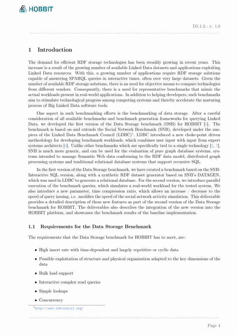
The DSB v2.0 parameters which need to be set in order to execute the benchmark are the following:3http://master.project-hobbit.eu/4http://hobbit_demo.openlinksw.com5https://github.com/hobbit-project/platform/wiki6https://project-hobbit.eu/challenges/mighty-storage-challenge2018/msc-tasks/#common-api7https://project-hobbit.eu/challenges/mighty-storage-challenge2018/msc-tasks/

#implementation-guidelines

. . . . . . . . . . . . . . . . . . . . . . . . . . . . . . . . . . . . . . . . . . . . . . . . . . . . . . . . . . . . . . . . . . . . . . . . . . . . . . . . . . . . . . . . . . . . . . . . . . . .

Page 7

D5.1.2 - v. 1.0. . . . . . . . . . . . . . . . . . . . . . . . . . . . . . . . . . . . . . . . . . . . . . . . . . . . . . . . . . . . . . . . . . . . . . . . . . . . . . . . . . . . . . . . . . . . . . . . . . . .

• Number of operations: The user must provide the total number of SPARQL queries (SELECTand INSERT) that should be executed against the tested system.

• Scale factor: DSB can be executed using different sizes of the dataset, i.e. with different scalefactors. The total number of triples per scale factor, along with several other properties of thedataset, are available in D5.1.1 [6].

• Seed: The user has to specify the seed for generating the pseudo-random numbers used fornon-deterministic selection of query substitution parameters.

• Time compression ratio (TCR): This value is used for "squeezing" together or "stretching"apart the queries of the workload, thus making it more or less demanding. The parameter isexplained in Section 3.

• Sequential Tasks: This check-box is disabled by default, and this means that the multithreadedapproach of the benchmark will be applied. We did not want to remove all useful features ofDSB v1.0, and therefore we provided an option to integrate them into DSB v2.0. If the check-box is enabled, the queries will be submitted to the tested system sequentially, one query afterthe other. This option is very useful when someone wants to compare systems with similarperformance results. For example, we did a lot of internal experiments comparing Virtuoso v7.2against Virtuoso v8.0, in order to track the performance of the system across versions. Withusing DSB v2.0, we were unable to notice some minor performance differences between these twosystems, because there is a lot of compensation between queries running at the same time. So,for a finer comparison between similar systems, or between different configurations of a singlesystem, this option is very useful. If this option is enabled, the Time Compression Ratio will beignored, thus the Throughput KPI will be relevant.

• Enable/Disable Query Type: This parameter controls if all query types should be includedin the workload. There are different scenarios where it would be useful to disable specific querytype(s) for the upcoming experiment, e.g. when a system is unable to cope with a specific typeof query, or it takes too long to process it. If a user does not want to invalidate all other resultsby running the problem-inducing queries as well, this option can be applied. By default, allquery types are enabled and a user can provide a string for this parameter containing ’0’ atthe position corresponding to the query type that should be disabled. For example, the string’01100’ will disable Q1, Q4 and Q5 in the experiment, while all the other will be enabled. Itwould be easier for the user to have a separate check-box for each query type that should beincluded in the workload, but it would result in too many benchmark parameters; an unwelcomeUI complication.

• Warm-up Percent: This parameter presents the percentage of total number of operations thatshould be used in the warm-up phase. These queries will not be evaluated later, and their purposeis only for system warm-up.

Figure 1 illustrates an example configuration of the Data Storage benchmark.

4.2 Components

Here, a brief description of the main components of the Data Storage benchmark is given, highlightingthe differences compared to the first version. A detailed presentation of the first version of DSB isprovided in D5.1.1 [6]. The implementation of the components can be found as part of the public

. . . . . . . . . . . . . . . . . . . . . . . . . . . . . . . . . . . . . . . . . . . . . . . . . . . . . . . . . . . . . . . . . . . . . . . . . . . . . . . . . . . . . . . . . . . . . . . . . . . .

Page 8

D5.1.2 - v. 1.0. . . . . . . . . . . . . . . . . . . . . . . . . . . . . . . . . . . . . . . . . . . . . . . . . . . . . . . . . . . . . . . . . . . . . . . . . . . . . . . . . . . . . . . . . . . . . . . . . . . .

Figure 1: Example Values for the DSB Parameters.

GitHub project8. The current implementation is in the master branch, but the previous versions aretagged with specific tags: v1.0, v1.1 and v1.2.

4.2.1 Benchmark Controller

The Benchmark Controller is the main component used to create and synchronize the other componentsof the benchmark. During the initialization phase, it gathers parameters from the Platform Controller,provided by a platform user, necessary to initialize the other components. Then the BenchmarkController executes the Data Storage benchmark by sending start signals to the Data Generator andthe Task Generator. When they are done, it creates the Evaluation Module of the benchmark, waits forit to finish and sends the received evaluation results of the benchmark to the Platform Storage. Fromthere, the platform can read the results, and present them to the user. This is a common scenario forthe controller component - the same scenario is implemented by all other benchmarks in the platform.This is the reason why this component has been undergone only minimal changes from DSB v1.0 toDSB v2.0. These minimal changes are related to using and passing the new DSB parameters.

4.2.2 Data Generator

The Data Generator is the component responsible for providing the dataset. Due to the nature of thesynthetic RDF dataset(s) generated with our DSB DATAGEN, there is no need to generate them foreach benchmark run separately. Additionally, the generation of the larger datasets can take a coupleof hours. So, instead, DSB uses pre-generated datasets when used within the HOBBIT platform [6].After the initialization phase, the Data Generator is aware of the designated scale factor, downloadsthe specified dataset and sends it to the System Adapter to be bulk loaded. When it receives the signalindicating that the bulk loading phase is finished, it starts sending the dataset to the Task Generator,

8https://github.com/hobbit-project/DataStorageBenchmark

. . . . . . . . . . . . . . . . . . . . . . . . . . . . . . . . . . . . . . . . . . . . . . . . . . . . . . . . . . . . . . . . . . . . . . . . . . . . . . . . . . . . . . . . . . . . . . . . . . . .

Page 9

D5.1.2 - v. 1.0. . . . . . . . . . . . . . . . . . . . . . . . . . . . . . . . . . . . . . . . . . . . . . . . . . . . . . . . . . . . . . . . . . . . . . . . . . . . . . . . . . . . . . . . . . . . . . . . . . . .

based on which it prepares the queries. The main differences introduced in the second version of thebenchmark for this component are related to the ability of generating more datasets of larger scales,and providing the relevant data to the Task Generator needed for queries, instead of sending the pre-calculated queries to it. This way, the Task Generator has the freedom to generate the queries byitself, opening up opportunities for more realistic workloads.

4.2.3 Task Generator

The Task Generator is the component responsible for creating the workload. It creates the tasks, i.e.the SPARQL SELECT and INSERT queries, based on the incoming data. The deliverable for the firstversion of the benchmark explained two approaches related to the process of checking the correctnessof the query results, and gave the rationale for using a pre-calculated set of results [6]. This componentreceives the data from the Data Generator, prepares the queries, retrieves the pre-calculated answersto them and then sends the queries to the System Adapter, and the answers to the Evaluate Storage.Compared to the DSB v1.0, this component has gone through a significant amount of changes. In thefirst version we use sequential tasks, i.e. the Task Generator sends the tasks one by one, waits for thesystem under test to process a task in full before sending the next one to the System Adapter. This isdone by synchronizing the Task Generator and the Evaluation Storage. In the second version of DSB,we have two types of Task Generators: one which is very similar to the Task Generator from DSB v1.0where sequential tasks are used, and a second one which runs the tasks in parallel and is more realisticand more useful for comparing different systems.

The Task Generator of DSB 2.0 does not synchronize with the other components - the queries aresubmitted according to the specified workload which encompasses the real-world frequencies, distri-butions and mutual ratios of the separate queries. The behavior of the Task Generator in this phaseis also affected by the designated time compression ratio, which provides an additional way of testingthe scalability, as we explained before. Additionally, the Task Generator of DSB 2.0 implements thepossibility to disable one or more types of queries, in order to get a workload without them. As wealready pointed out, this is very useful for debugging and tweaking the system under test.

The following is a pseudo-code for the most important method of the Task Generator, responsiblefor generating the tasks:

protected void generateTask(byte[] data) {//convert the data received from the Data Generator into suitable formString dataString = convert(data);

// extract and prepare the exact time when the task has to be submittedlong newSimulatedTime = extract_and_prepare(dataString);// current timelong newRealTime = System.currentTimeMillis();

// wait for the right time having in mind the time compression ratiolong waitingTime = calculate_wait_time(newSimulatedTime, newRealTime, tcr)wait(waitingTime);

// prepare SPARQL INSERT queryString updateString = prepare_update(dataString);

// if that type is not disabled, submit the query

. . . . . . . . . . . . . . . . . . . . . . . . . . . . . . . . . . . . . . . . . . . . . . . . . . . . . . . . . . . . . . . . . . . . . . . . . . . . . . . . . . . . . . . . . . . . . . . . . . . .

Page 10

D5.1.2 - v. 1.0. . . . . . . . . . . . . . . . . . . . . . . . . . . . . . . . . . . . . . . . . . . . . . . . . . . . . . . . . . . . . . . . . . . . . . . . . . . . . . . . . . . . . . . . . . . . . . . . . . . .

if (!disabled(update_type(updateString)))sendTaskToSystemAdapter(updateString);

// for all SPARQL SELECT queriesfor (type : select_types) {

// if it is the right time to submit the specific query type according to workload// and the query type is not disabledif (can_submit(type) && !disable(type)) {

// prepare text of a queryString selectString = prepareSelectQuery(type);// prepare answer of a queryString answer = prepareAnswer(selectString);

// sent query to the System AdaptersendTaskToSystemAdapter(taskIdString, selectString);// sent answer and the timestamp of the current time to the Evaluation StoragesendTaskToEvalStorage(current_timestamp(), answer);

}}

}

4.2.4 System Adapter

The System Adapter is a component which enables the communication between the benchmark andthe system under test. It receives data from Data Generator, loads it into the system, and then informsthe other components that it is ready to start executing the SPARQL queries. It then gets the queriesfrom the Task Generator and forwards them to the system being tested. The results of the queriesare sent to the Evaluation Storage for validation and evaluation, where the correctness, timeliness andother significant characteristics are measured.

We developed a couple of instances of the System Adapter. One of them is used for our baselineimplementation of DSB, for which we used the Virtuoso open-source version (VOS). We developedother instances for the commercial versions of Virtuoso v7.2, v7.5, v8.0 and v8.1 (beta). For eachof them the System Adapter is mostly the same, and it is part of the same Docker container as thesystem.

This benchmark is a part of the Mighty Storage Challenge (MOCHA), where we have a commonAPI for all benchmarks which comprise it (Section 4.2.6). That means that all systems which followthe same API could be tested against any benchmark from the MOCHA challenge (ODIN, DSB,Versioning, and Faceted benchmark). Practically, all the systems developed as a baseline for any ofthese tasks could be used with our benchmark, and vice versa. Apart from our systems, we testedBlazegraph, GraphDB and Apache Jena Fuseki, for which the system adapters were developed withindifferent work packages.

4.2.5 Evaluation Module

The Evaluation Module is the component which validates and evaluates the results received from thebenchmarked system. The answers to the queries are pre-calculated using the golden standard, andthen are compared to the actual answers that the benchmarked system provided. For each SPARQL

. . . . . . . . . . . . . . . . . . . . . . . . . . . . . . . . . . . . . . . . . . . . . . . . . . . . . . . . . . . . . . . . . . . . . . . . . . . . . . . . . . . . . . . . . . . . . . . . . . . .

Page 11

D5.1.2 - v. 1.0. . . . . . . . . . . . . . . . . . . . . . . . . . . . . . . . . . . . . . . . . . . . . . . . . . . . . . . . . . . . . . . . . . . . . . . . . . . . . . . . . . . . . . . . . . . . . . . . . . . .

query, the Evaluation Storage saves the execution start-time and end-time, along with the expectedresult set. Based on these measurements, this component calculates all specified key performanceindicators (KPIs) described in Section 3.1, and sends them to the platform (as an RDF model) to bepresented to the user.

The KPIs of the experiments running against our second version of DSB are the ones describedin Section 3.1, and they can be summarized and compared within the platform results page.

4.2.6 Common API

In the scope of the HOBBIT project, we have 4 different benchmarks that evaluate the performanceof triple stores from different aspects:

• ODIN: An RDF data ingestion benchmark that measures how well systems can ingest streamsof RDF data.

• DSB: The Data storage benchmark that measures how data stores perform with different typesof queries.

• Versioning Benchmark: The Versioning benchmark measures how well versioning and archivingsystems for Linked Data perform when they store multiple versions of large datasets.

• Faceted Benchmark: The Browsing Benchmark checks existing solutions for how well they sup-port applications that need browsing through large datasets.

We developed the components of these benchmarks following the common API that we jointly ap-proved. All systems should follow the same API, thus will be ready to be evaluated with any of thesebenchmarks. In this section, we present the common API.

A SPARQL based system has four phases during the benchmarking:

1. Initialization phase: As every system, it has to initialize itself, e.g., start needed components,load configurations, etc. This phase ends as soon as it sends the SYSTEM_READY_SIGNAL on thecommand queue (as described in the wiki and implemented in the AbstractSystemAdapter9).

2. Loading phase: After the system is running and the benchmark is started, it can receive datafrom the data queue which it should load into its triple store. This can be done as bulkload. The benchmark controller will send a BULK_LOAD_DATA_GEN_FINISHED signal on the com-mand queue when the data from the data generator has been placed in the data queue. TheBULK_LOAD_DATA_GEN_FINISHED message comes with an integer value (4 bytes) as additionaldata, representing the number of data messages the system adapter should get from the dataqueue. Note that the benchmark controller might have to collect the number of generated datamessages from the data generators. In addition, the BULK_LOAD_DATA_GEN_FINISHED messagescontains a flag that determines whether there are more data that have to be sent by the bench-mark controller. This flag lets the system enter the querying phase, or makes it wait for addi-tional data to come. More specifically, the system will read the remaining data from the dataqueue, bulk load it into the store and send a BULK_LOADING_DATA_FINISHED signal on the com-mand queue to the benchmark controller, to indicate that it has finished the loading. If the

9https://github.com/hobbit-project/core/blob/master/src/main/java/org/hobbit/core/components/AbstractSystemAdapter.java

. . . . . . . . . . . . . . . . . . . . . . . . . . . . . . . . . . . . . . . . . . . . . . . . . . . . . . . . . . . . . . . . . . . . . . . . . . . . . . . . . . . . . . . . . . . . . . . . . . . .

Page 12

D5.1.2 - v. 1.0. . . . . . . . . . . . . . . . . . . . . . . . . . . . . . . . . . . . . . . . . . . . . . . . . . . . . . . . . . . . . . . . . . . . . . . . . . . . . . . . . . . . . . . . . . . . . . . . . . . .

flag of BULK_LOAD_DATA_GEN_FINISHED command was false, it waits for the next set of data tocome, bulk load it into the store and send the BULK_LOADING_DATA_FINISHED signal again onthe command queue. If the flag is true it can proceed to the querying phase. The values of theaforementioned commands are:

BULK_LOADING_DATA_FINISHED = (byte) 150;BULK_LOAD_DATA_GEN_FINISHED = (byte) 151;

The data received at that time is structured in the following way:

• Integer value (4 bytes) containing the length of the graph URI

• Graph URI (UTF-8 encoded String)

• NTriples (UTF-8 encoded String; the rest of the package/data stream)

Example workflow:

01. lastBulkLoad = false02. while lastBulkLoad is false do03. numberOfMessages = X04. benchmark sends data to system05. if there are no more data for sending then06. lastBulkLoad = true07. end if08. benchmark sends BULK_LOAD_DATA_GEN_FINISHED { numberOfMessages,lastBulkLoad }09. system loads data10. system sends BULK_LOADING_DATA_FINISHED11. done12. system enters querying phase

For the benchmarks that measure the time it takes a system to load the data, the times fromstep 8 to 10 are measured.

3. Querying phase: During this phase the system can get two types of input:

• Data from the data queue that should be inserted into the store in the form of INSERTSPARQL queries.

• Tasks from the task queue, i.e., SPARQL queries (SELECT, INSERT, etc.) that it has toexecute. The results for the single tasks (in JSON format) have to be sent together withthe id of the task to the result queue.

4. Termination phase: As described in the wiki, the third phase ends when the system receives theTASK_GENERATION_FINISHED command and has consumed all the remaining messages from thetask queue. (The AbstractSystemAdapter already contains this step.)

5 Evaluation

As we mentioned in Section 4.2.4, in the scope of the HOBBIT project we developed four differentbaseline systems implementing the common API, and that they could be tested against DSB. This

. . . . . . . . . . . . . . . . . . . . . . . . . . . . . . . . . . . . . . . . . . . . . . . . . . . . . . . . . . . . . . . . . . . . . . . . . . . . . . . . . . . . . . . . . . . . . . . . . . . .

Page 13

D5.1.2 - v. 1.0. . . . . . . . . . . . . . . . . . . . . . . . . . . . . . . . . . . . . . . . . . . . . . . . . . . . . . . . . . . . . . . . . . . . . . . . . . . . . . . . . . . . . . . . . . . . . . . . . . . .

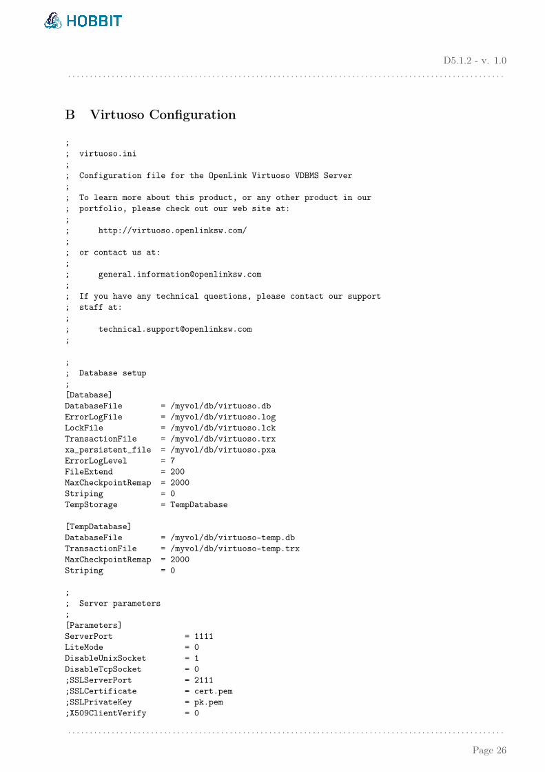
section should not be considered as a comparison of the tested systems, for two reasons: (a) theexperiments we ran were intended to prove that our benchmark works as intended and expected, and(b) the baseline systems developed within other workpackages are not capable of answering queriesin reasonable time, even for the smallest dataset (also verified with the MOCHA challenge results inSection 6). Because of that, in the experiments that follow we use Virtuoso open-source (VOS) as thesystem under test. The version of VOS is 07.20.3217 and its configuration file is given in Appendix B.The experiments presented in this section were executed on the HOBBIT platform.

5.1 Sequential Tasks

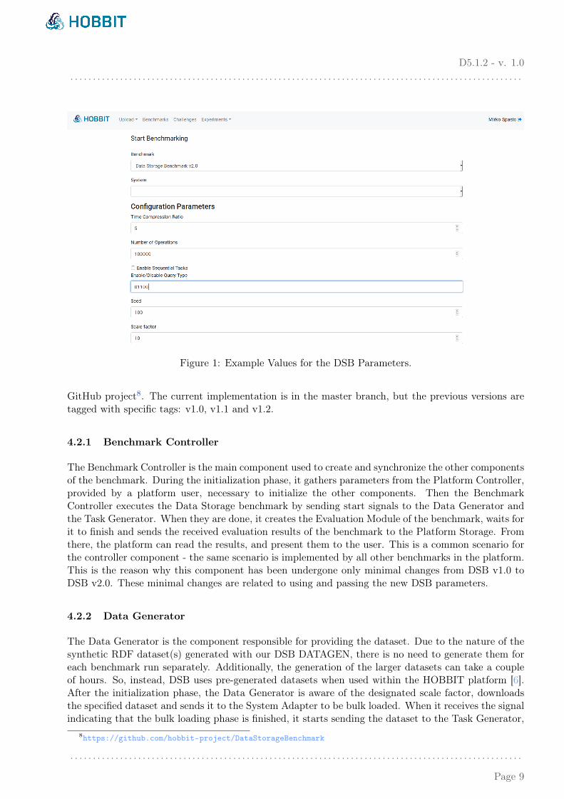
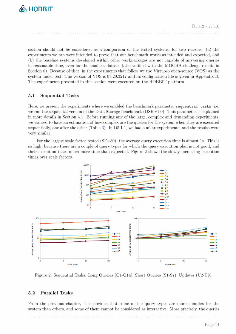
Here, we present the experiments where we enabled the benchmark parameter sequential tasks, i.e.we ran the sequential version of the Data Storage benchmark (DSB v1.0). This parameter is explainedin more details in Section 4.1. Before running any of the large, complex and demanding experiments,we wanted to have an estimation of how complex are the queries for the system when they are executedsequentially, one after the other (Table 3). In D5.1.1, we had similar experiments, and the results werevery similar.

For the largest scale factor tested (SF=30), the average query execution time is almost 1s. This isso high, because there are a couple of query types for which the query execution plan is not good, andtheir execution takes much more time than expected. Figure 2 shows the slowly increasing executiontimes over scale factors.

Figure 2: Sequential Tasks: Long Queries (Q1-Q14), Short Queries (S1-S7), Updates (U2-U8).

5.2 Parallel Tasks

From the previous chapter, it is obvious that some of the query types are more complex for thesystem than others, and some of them cannot be considered as interactive. More precisely, the queries

. . . . . . . . . . . . . . . . . . . . . . . . . . . . . . . . . . . . . . . . . . . . . . . . . . . . . . . . . . . . . . . . . . . . . . . . . . . . . . . . . . . . . . . . . . . . . . . . . . . .

Page 14

D5.1.2 - v. 1.0. . . . . . . . . . . . . . . . . . . . . . . . . . . . . . . . . . . . . . . . . . . . . . . . . . . . . . . . . . . . . . . . . . . . . . . . . . . . . . . . . . . . . . . . . . . . . . . . . . . .

themselves are developed to be interactive, and the audited results of non-RDF systems tested withinthe LDBC project against the SQL version of these queries are the proof of that10. But here, thetested triple stores are not capable of executing these queries in a short enough time so that they canbe considered as interactive (i.e. execute in less than a couple of seconds). If we include these querytypes in the real workload, where the queries are submitted very fast, and several at once, they willtake a lot of time to execute, they will pile up, and after some time there will be lot of them executingat once, occupying all hardware resources and paralyzing the newly arrived queries. The delay will beincreasing constantly, thus invalidating the whole experiment.

With this in mind, we decided to temporarily disable these long lasting query types, and keep onlyfast ones for the following set of experiments. We achieved this by setting the benchmark parameterEnable/Disable Query Type to 01100111011010111111111111111. We executed VOS against DSB,while varying different parameters:

• Scale Factors (SF): 1, 3, 10, 30

• Time Compression Ratio (TCR): 0.03, 0.1, 0.3, 1, 3, 10, 30, 100, 300

In all experiments, the number of operations (SPARQL queries) is 20000, out of which 20% are usedfor system warm-up.

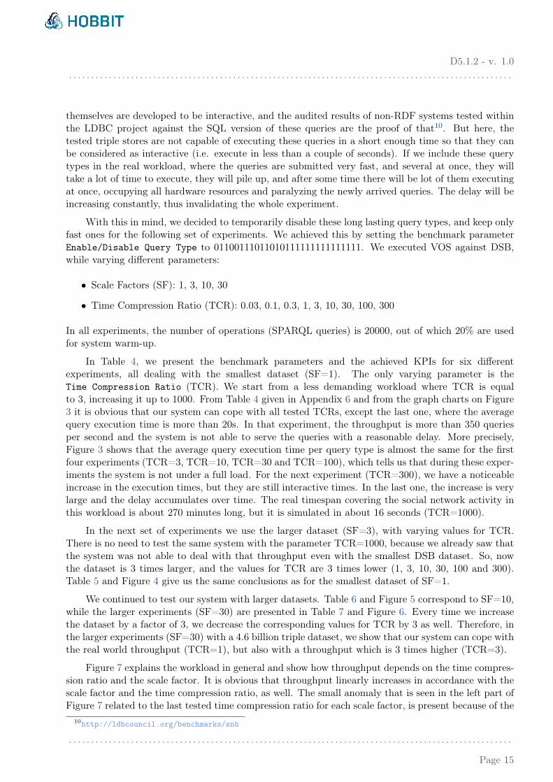
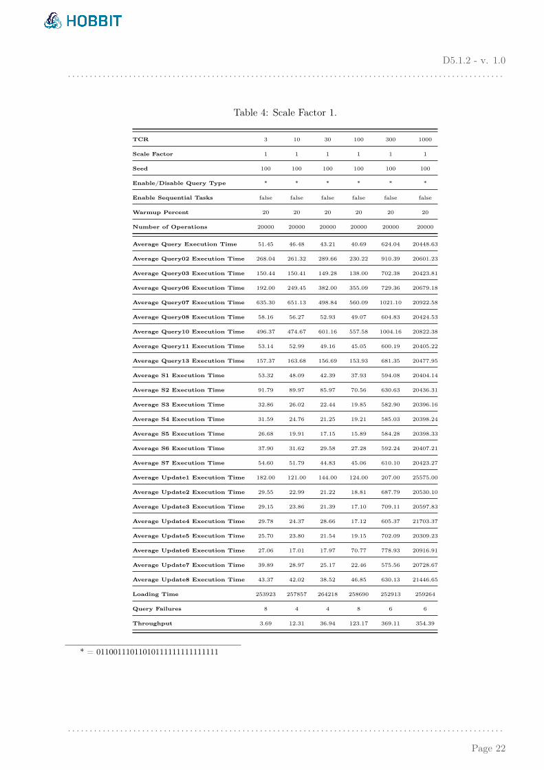
In Table 4, we present the benchmark parameters and the achieved KPIs for six differentexperiments, all dealing with the smallest dataset (SF=1). The only varying parameter is theTime Compression Ratio (TCR). We start from a less demanding workload where TCR is equalto 3, increasing it up to 1000. From Table 4 given in Appendix 6 and from the graph charts on Figure3 it is obvious that our system can cope with all tested TCRs, except the last one, where the averagequery execution time is more than 20s. In that experiment, the throughput is more than 350 queriesper second and the system is not able to serve the queries with a reasonable delay. More precisely,Figure 3 shows that the average query execution time per query type is almost the same for the firstfour experiments (TCR=3, TCR=10, TCR=30 and TCR=100), which tells us that during these exper-iments the system is not under a full load. For the next experiment (TCR=300), we have a noticeableincrease in the execution times, but they are still interactive times. In the last one, the increase is verylarge and the delay accumulates over time. The real timespan covering the social network activity inthis workload is about 270 minutes long, but it is simulated in about 16 seconds (TCR=1000).

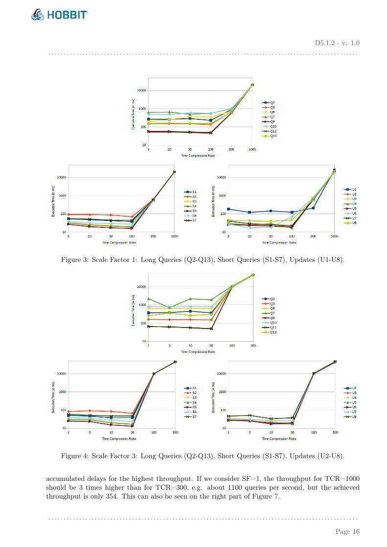
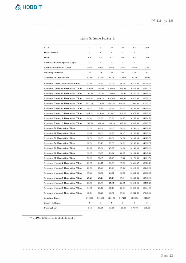
In the next set of experiments we use the larger dataset (SF=3), with varying values for TCR.There is no need to test the same system with the parameter TCR=1000, because we already saw thatthe system was not able to deal with that throughput even with the smallest DSB dataset. So, nowthe dataset is 3 times larger, and the values for TCR are 3 times lower (1, 3, 10, 30, 100 and 300).Table 5 and Figure 4 give us the same conclusions as for the smallest dataset of SF=1.

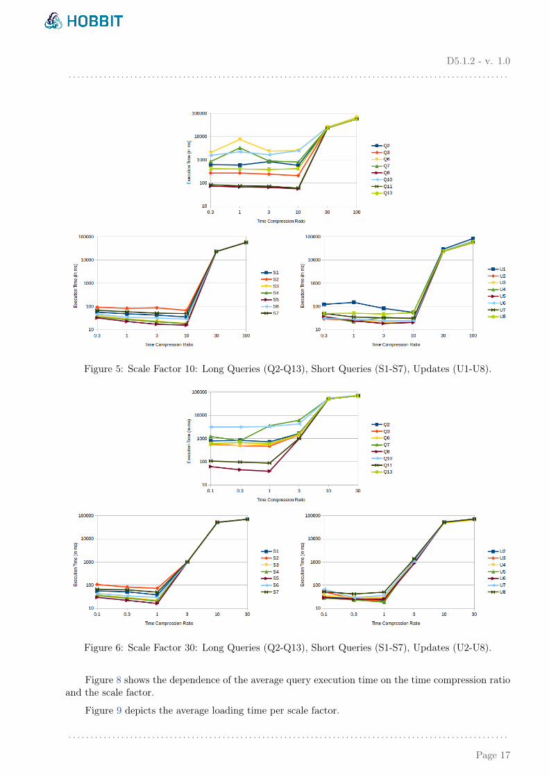
We continued to test our system with larger datasets. Table 6 and Figure 5 correspond to SF=10,while the larger experiments (SF=30) are presented in Table 7 and Figure 6. Every time we increasethe dataset by a factor of 3, we decrease the corresponding values for TCR by 3 as well. Therefore, inthe larger experiments (SF=30) with a 4.6 billion triple dataset, we show that our system can cope withthe real world throughput (TCR=1), but also with a throughput which is 3 times higher (TCR=3).

Figure 7 explains the workload in general and show how throughput depends on the time compres-sion ratio and the scale factor. It is obvious that throughput linearly increases in accordance with thescale factor and the time compression ratio, as well. The small anomaly that is seen in the left part ofFigure 7 related to the last tested time compression ratio for each scale factor, is present because of the

10http://ldbcouncil.org/benchmarks/snb

. . . . . . . . . . . . . . . . . . . . . . . . . . . . . . . . . . . . . . . . . . . . . . . . . . . . . . . . . . . . . . . . . . . . . . . . . . . . . . . . . . . . . . . . . . . . . . . . . . . .

Page 15

D5.1.2 - v. 1.0. . . . . . . . . . . . . . . . . . . . . . . . . . . . . . . . . . . . . . . . . . . . . . . . . . . . . . . . . . . . . . . . . . . . . . . . . . . . . . . . . . . . . . . . . . . . . . . . . . . .

Figure 3: Scale Factor 1: Long Queries (Q2-Q13), Short Queries (S1-S7), Updates (U1-U8).

Figure 4: Scale Factor 3: Long Queries (Q2-Q13), Short Queries (S1-S7), Updates (U2-U8).

accumulated delays for the highest throughput. If we consider SF=1, the throughput for TCR=1000should be 3 times higher than for TCR=300, e.g. about 1100 queries per second, but the achievedthroughput is only 354. This can also be seen on the right part of Figure 7.

. . . . . . . . . . . . . . . . . . . . . . . . . . . . . . . . . . . . . . . . . . . . . . . . . . . . . . . . . . . . . . . . . . . . . . . . . . . . . . . . . . . . . . . . . . . . . . . . . . . .

Page 16

D5.1.2 - v. 1.0. . . . . . . . . . . . . . . . . . . . . . . . . . . . . . . . . . . . . . . . . . . . . . . . . . . . . . . . . . . . . . . . . . . . . . . . . . . . . . . . . . . . . . . . . . . . . . . . . . . .

Figure 5: Scale Factor 10: Long Queries (Q2-Q13), Short Queries (S1-S7), Updates (U1-U8).

Figure 6: Scale Factor 30: Long Queries (Q2-Q13), Short Queries (S1-S7), Updates (U2-U8).

Figure 8 shows the dependence of the average query execution time on the time compression ratioand the scale factor.

Figure 9 depicts the average loading time per scale factor.

. . . . . . . . . . . . . . . . . . . . . . . . . . . . . . . . . . . . . . . . . . . . . . . . . . . . . . . . . . . . . . . . . . . . . . . . . . . . . . . . . . . . . . . . . . . . . . . . . . . .

Page 17

D5.1.2 - v. 1.0. . . . . . . . . . . . . . . . . . . . . . . . . . . . . . . . . . . . . . . . . . . . . . . . . . . . . . . . . . . . . . . . . . . . . . . . . . . . . . . . . . . . . . . . . . . . . . . . . . . .

Figure 7: Throughput by Time Compression Ratio (left) and by Scale Factor (right).

Figure 8: Average Query Execution Time by Time Compression Ratio (left) and by Scale Factor (right).

Figure 9: Average Loading Time by Scale Factor.

6 MOCHA Preliminary Challenge Results

At the end of the reporting period for the deliverable, the Data Storage Benchmark was part of theMighty Storage Challenge (MOCHA) 201811, at ESWC 201812. The challenge consisted of four tasks,and DSB was Task 2. The benchmark had a defined maximum time for the experiment of 3 hours.Table 2 shows the configuration for DSB at MOCHA 2018.

For the participation in Task 2 of MOCHA 2018, i.e. for the Data Storage Benchmark, five systemsapplied and were submitted: Virtuoso 7.2 Open-Source Edition by OpenLink Software, Virtuoso 8.0

11https://project-hobbit.eu/challenges/mighty-storage-challenge2018/12https://2018.eswc-conferences.org/

. . . . . . . . . . . . . . . . . . . . . . . . . . . . . . . . . . . . . . . . . . . . . . . . . . . . . . . . . . . . . . . . . . . . . . . . . . . . . . . . . . . . . . . . . . . . . . . . . . . .

Page 18

D5.1.2 - v. 1.0. . . . . . . . . . . . . . . . . . . . . . . . . . . . . . . . . . . . . . . . . . . . . . . . . . . . . . . . . . . . . . . . . . . . . . . . . . . . . . . . . . . . . . . . . . . . . . . . . . . .

Commercial Edition by OpenLink Software, Blazegraph, GraphDB Free 8.5, and Apache Jena Fuseki3.6.0.

Table 2: MOCHA 2018 - DSB Configuration.

Parameter Value

Scale Factor 30

Number of operations 15000

Time Compression Ratio 0.5

Enable/Disable Query Type *

Seed 100

Sequential Tasks false

Warmup Percent 20

Unfortunately, Blazegraph, GraphDB and Jena Fuseki were not able to finish the experiment inthe requested time, i.e. it exhibited a timeout. Based on the results from the main KPIs (Figure 10)and the rest of the KPIs (Figure 11), the winning system for the task was Virtuoso 8.0 CommercialEdition by OpenLink Software.

Figure 10: MOCHA 2018 - Task 2: Short Queries and Updates

* = 01100111011010111111111111111

. . . . . . . . . . . . . . . . . . . . . . . . . . . . . . . . . . . . . . . . . . . . . . . . . . . . . . . . . . . . . . . . . . . . . . . . . . . . . . . . . . . . . . . . . . . . . . . . . . . .

Page 19

D5.1.2 - v. 1.0. . . . . . . . . . . . . . . . . . . . . . . . . . . . . . . . . . . . . . . . . . . . . . . . . . . . . . . . . . . . . . . . . . . . . . . . . . . . . . . . . . . . . . . . . . . . . . . . . . . .

Figure 11: MOCHA 2018 - Task 2: Average Query Execution Time per Query Type

References

[1] Renzo Angles, Peter Boncz, Josep Larriba-Pey, Irini Fundulaki, Thomas Neumann, Orri Erling,Peter Neubauer, Norbert Martinez-Bazan, Venelin Kotsev, and Ioan Toma. The Linked DataBenchmark Council: A Graph and RDF Industry Benchmarking Effort. SIGMOD Rec., 43(1):27–31, May 2014.

[2] Christian Bizer and Andreas Schultz. The Berlin SPARQL Benchmark. Int. J. Semantic Web Inf.Syst., 5(2):1–24, 2009.

[3] Peter Boncz, Thomas Neumann, and Orri Erling. TPC-H Analyzed: Hidden Messages and LessonsLearned from an Influential Benchmark. In Revised Selected Papers of the 5th TPC Technology Con-ference on Performance Characterization and Benchmarking - Volume 8391, pages 61–76, Berlin,Heidelberg, 2014. Springer-Verlag.

[4] Orri Erling, Alex Averbuch, Josep Larriba-Pey, Hassan Chafi, Andrey Gubichev, Arnau Prat, Minh-Duc Pham, and Peter Boncz. The LDBC Social Network Benchmark: Interactive Workload. InProceedings of the 2015 ACM SIGMOD International Conference on Management of Data, pages619–630. ACM, 2015.

[5] Yuanbo Guo, Abir Qasem, Zhengxiang Pan, and Jeff Heflin. A Requirements Driven Frameworkfor Benchmarking Semantic Web Knowledge Base Systems. IEEE Transactions on Knowledge andData Engineering, 19(2):297–309, Feb 2007.

[6] Milos Jovanovik and Mirko Spasić. First Version of the Data Storage Bench-mark. https://project-hobbit.eu/wp-content/uploads/2017/06/D5.1.1_First_version_of_the_Data_Storage_Benchmark.pdf, May 2017. Project HOBBIT Deliverable 5.1.1.

[7] Venelin Kotsev, Nikos Minadakis, Vassilis Papakonstantinou, Orri Erling, Irini Fundulaki, andAtanas Kiryakov. Benchmarking RDF Query Engines: The LDBC Semantic Publishing Benchmark.In BLINK@ISWC, 2016.

[8] Janet Wiener and Nathan Bronson. Facebook’s Top Open Data Problems. https://research.fb.com/facebook-s-top-open-data-problems/, October 2014.

. . . . . . . . . . . . . . . . . . . . . . . . . . . . . . . . . . . . . . . . . . . . . . . . . . . . . . . . . . . . . . . . . . . . . . . . . . . . . . . . . . . . . . . . . . . . . . . . . . . .

Page 20

D5.1.2 - v. 1.0. . . . . . . . . . . . . . . . . . . . . . . . . . . . . . . . . . . . . . . . . . . . . . . . . . . . . . . . . . . . . . . . . . . . . . . . . . . . . . . . . . . . . . . . . . . . . . . . . . . .

A Tables

Table 3: Sequential Tasks.

Scale Factor 1 3 10 30

TCR 1 1 1 1

Seed 100 100 100 100

Enable/Disable Query Type - - - -

Enable Sequential Tasks true true true true

Number of Operations 20000 20000 20000 20000

Average Query Execution Time 78.14 187.35 379.25 899.42

Average Query01 Execution Time 3595.73 3906.22 6819.36 15088.27

Average Query02 Execution Time 224.82 426.72 550.97 669.51

Average Query03 Execution Time 111.19 118.74 218.19 524.94

Average Query04 Execution Time 891.63 4987.81 27899.67 91529.82

Average Query05 Execution Time 2881.18 21781.49 19201.00 35698.52

Average Query06 Execution Time 312.00 621.60 1895.40 496.60

Average Query07 Execution Time 432.12 1587.03 924.57 1753.32

Average Query08 Execution Time 38.83 47.73 68.15 70.04

Average Query09 Execution Time 8343.25 14961.38 32335.38 54364.00

Average Query10 Execution Time 544.94 781.56 1519.05 3307.79

Average Query11 Execution Time 31.99 39.20 49.83 76.11

Average Query12 Execution Time 198.22 235.18 336.18 432.32

Average Query13 Execution Time 126.53 305.73 398.48 638.28

Average Query14 Execution Time 1441.26 5282.79 13054.95 17006.48

Average S1 Execution Time 23.01 29.37 28.64 32.68

Average S2 Execution Time 54.54 60.83 67.64 77.79

Average S3 Execution Time 10.08 10.41 12.73 14.79

Average S4 Execution Time 8.40 8.85 9.94 11.50

Average S5 Execution Time 6.11 6.22 7.29 7.81

Average S6 Execution Time 14.57 14.04 14.76 19.49

Average S7 Execution Time 28.74 27.67 29.71 39.88

Average Update2 Execution Time 10.67 11.68 14.91 30.21

Average Update3 Execution Time 10.26 15.73 14.71 20.49

Average Update4 Execution Time 10.39 15.40 19.08 20.10

Average Update5 Execution Time 9.74 9.85 13.42 13.91

Average Update6 Execution Time 10.54 12.26 17.40 21.76

Average Update7 Execution Time 13.29 17.43 23.15 35.73

Average Update8 Execution Time 15.22 14.77 19.00 28.61

Loading Time 254592 319601 939616 3392135

Throughput 12.23 5.23 2.62 1.11

. . . . . . . . . . . . . . . . . . . . . . . . . . . . . . . . . . . . . . . . . . . . . . . . . . . . . . . . . . . . . . . . . . . . . . . . . . . . . . . . . . . . . . . . . . . . . . . . . . . .

Page 21

D5.1.2 - v. 1.0. . . . . . . . . . . . . . . . . . . . . . . . . . . . . . . . . . . . . . . . . . . . . . . . . . . . . . . . . . . . . . . . . . . . . . . . . . . . . . . . . . . . . . . . . . . . . . . . . . . .

Table 4: Scale Factor 1.

TCR 3 10 30 100 300 1000

Scale Factor 1 1 1 1 1 1

Seed 100 100 100 100 100 100

Enable/Disable Query Type * * * * * *

Enable Sequential Tasks false false false false false false

Warmup Percent 20 20 20 20 20 20

Number of Operations 20000 20000 20000 20000 20000 20000

Average Query Execution Time 51.45 46.48 43.21 40.69 624.04 20448.63

Average Query02 Execution Time 268.04 261.32 289.66 230.22 910.39 20601.23

Average Query03 Execution Time 150.44 150.41 149.28 138.00 702.38 20423.81

Average Query06 Execution Time 192.00 249.45 382.00 355.09 729.36 20679.18

Average Query07 Execution Time 635.30 651.13 498.84 560.09 1021.10 20922.58

Average Query08 Execution Time 58.16 56.27 52.93 49.07 604.83 20424.53

Average Query10 Execution Time 496.37 474.67 601.16 557.58 1004.16 20822.38

Average Query11 Execution Time 53.14 52.99 49.16 45.05 600.19 20405.22

Average Query13 Execution Time 157.37 163.68 156.69 153.93 681.35 20477.95

Average S1 Execution Time 53.32 48.09 42.39 37.93 594.08 20404.14

Average S2 Execution Time 91.79 89.97 85.97 70.56 630.63 20436.31

Average S3 Execution Time 32.86 26.02 22.44 19.85 582.90 20396.16

Average S4 Execution Time 31.59 24.76 21.25 19.21 585.03 20398.24

Average S5 Execution Time 26.68 19.91 17.15 15.89 584.28 20398.33

Average S6 Execution Time 37.90 31.62 29.58 27.28 592.24 20407.21

Average S7 Execution Time 54.60 51.79 44.83 45.06 610.10 20423.27

Average Update1 Execution Time 182.00 121.00 144.00 124.00 207.00 25575.00

Average Update2 Execution Time 29.55 22.99 21.22 18.81 687.79 20530.10

Average Update3 Execution Time 29.15 23.86 21.39 17.10 709.11 20597.83

Average Update4 Execution Time 29.78 24.37 28.66 17.12 605.37 21703.37

Average Update5 Execution Time 25.70 23.80 21.54 19.15 702.09 20309.23

Average Update6 Execution Time 27.06 17.01 17.97 70.77 778.93 20916.91

Average Update7 Execution Time 39.89 28.97 25.17 22.46 575.56 20728.67

Average Update8 Execution Time 43.37 42.02 38.52 46.85 630.13 21446.65

Loading Time 253923 257857 264218 258690 252913 259264

Query Failures 8 4 4 8 6 6

Throughput 3.69 12.31 36.94 123.17 369.11 354.39

* = 01100111011010111111111111111

. . . . . . . . . . . . . . . . . . . . . . . . . . . . . . . . . . . . . . . . . . . . . . . . . . . . . . . . . . . . . . . . . . . . . . . . . . . . . . . . . . . . . . . . . . . . . . . . . . . .

Page 22

D5.1.2 - v. 1.0. . . . . . . . . . . . . . . . . . . . . . . . . . . . . . . . . . . . . . . . . . . . . . . . . . . . . . . . . . . . . . . . . . . . . . . . . . . . . . . . . . . . . . . . . . . . . . . . . . . .

Table 5: Scale Factor 3.

TCR 1 3 10 30 100 300

Scale Factor 1 1 1 1 1 1

Seed 100 100 100 100 100 100

Enable/Disable Query Type * * * * * *

Enable Sequential Tasks false false false false false false

Warmup Percent 20 20 20 20 20 20

Number of Operations 20000 20000 20000 20000 20000 20000

Average Query Execution Time 61.48 54.47 53.04 48.00 10215.03 45024.27

Average Query02 Execution Time 374.60 382.68 456.68 369.02 10422.48 45291.61

Average Query03 Execution Time 161.94 157.94 158.00 152.53 10220.22 44870.34

Average Query06 Execution Time 645.91 645.18 657.09 654.09 10817.09 45908.64

Average Query07 Execution Time 2231.96 714.86 2213.90 1949.81 11332.00 47582.35

Average Query08 Execution Time 66.85 61.27 57.39 49.83 10162.09 44964.15

Average Query10 Execution Time 824.21 819.09 825.07 819.23 10973.86 45705.73

Average Query11 Execution Time 64.14 62.90 55.89 48.17 10153.89 44926.73

Average Query13 Execution Time 255.48 364.93 265.93 302.41 10433.94 45217.93

Average S1 Execution Time 51.31 46.51 37.68 38.53 10141.17 44930.25

Average S2 Execution Time 83.47 92.60 84.95 66.47 10187.32 44967.41

Average S3 Execution Time 32.01 30.38 21.04 16.90 10139.24 44929.59

Average S4 Execution Time 30.04 29.19 20.06 16.61 10142.30 44932.97

Average S5 Execution Time 24.92 23.61 15.39 13.00 10142.86 44933.69

Average S6 Execution Time 38.05 35.95 28.32 23.65 10152.35 44945.21

Average S7 Execution Time 58.99 51.85 47.15 47.20 10170.24 44964.51

Average Update2 Execution Time 28.05 24.77 20.30 17.98 10391.47 45623.29

Average Update3 Execution Time 28.96 25.46 19.10 17.16 10415.29 45140.80

Average Update4 Execution Time 37.40 31.57 24.37 18.53 10052.63 43690.07

Average Update5 Execution Time 27.26 25.14 17.43 17.34 10435.24 45543.89

Average Update6 Execution Time 28.63 26.63 17.67 20.05 10012.84 42705.29

Average Update7 Execution Time 34.95 28.71 27.49 25.61 10395.02 45644.99

Average Update8 Execution Time 46.74 51.27 33.71 37.61 10622.35 47740.81

Loading Time 316664 316494 328193 317247 322298 324097

Query Failures 7 8 7 8 3 6

Throughput 3.42 10.27 34.25 102.80 270.79 181.21

* = 01100111011010111111111111111

. . . . . . . . . . . . . . . . . . . . . . . . . . . . . . . . . . . . . . . . . . . . . . . . . . . . . . . . . . . . . . . . . . . . . . . . . . . . . . . . . . . . . . . . . . . . . . . . . . . .

Page 23

D5.1.2 - v. 1.0. . . . . . . . . . . . . . . . . . . . . . . . . . . . . . . . . . . . . . . . . . . . . . . . . . . . . . . . . . . . . . . . . . . . . . . . . . . . . . . . . . . . . . . . . . . . . . . . . . . .

Table 6: Scale Factor 10.

TCR 0.3 1 3 10 30 100

Scale Factor 1 1 1 1 1 1

Seed 100 100 100 100 100 100

Enable/Disable Query Type * * * * * *

Enable Sequential Tasks false false false false false false

Warmup Percent 20 20 20 20 20 20

Number of Operations 20000 20000 20000 20000 20000 20000

Average Query Execution Time 71.31 79.07 59.40 57.96 23338.14 57513.94

Average Query02 Execution Time 615.01 589.00 831.86 570.33 23668.28 57880.89

Average Query03 Execution Time 267.78 267.13 239.50 206.34 23407.41 57356.19

Average Query06 Execution Time 2064.00 7489.18 2358.73 2460.00 25537.91 67469.82

Average Query07 Execution Time 835.83 3256.71 880.54 797.68 23919.01 58094.57

Average Query08 Execution Time 72.89 67.13 64.36 55.85 23276.22 57441.14

Average Query10 Execution Time 1549.42 2193.72 1645.80 2457.39 24820.22 59606.41

Average Query11 Execution Time 83.51 75.18 72.02 59.97 23261.33 57395.05

Average Query13 Execution Time 410.22 401.34 379.43 413.39 23692.61 57717.26

Average S1 Execution Time 56.47 47.90 42.35 34.94 23249.06 57398.98

Average S2 Execution Time 92.34 82.38 87.02 67.44 23290.71 57442.18

Average S3 Execution Time 40.88 29.49 23.06 18.50 23246.12 57399.56

Average S4 Execution Time 35.65 27.02 21.79 18.05 23249.51 57403.08

Average S5 Execution Time 32.03 22.40 17.05 15.58 23250.32 57404.22

Average S6 Execution Time 46.36 34.00 31.79 28.21 23260.46 57413.95

Average S7 Execution Time 68.28 58.64 51.07 49.07 23279.05 57434.54

Average Update2 Execution Time 122.00 149.00 82.00 55.00 29279.00 84379.00

Average Update2 Execution Time 29.17 24.67 20.79 21.01 23495.05 57514.88

Average Update3 Execution Time 36.04 24.72 20.62 21.05 23188.52 56102.77

Average Update4 Execution Time 36.15 21.38 34.08 29.85 24836.38 64149.62

Average Update5 Execution Time 36.49 23.79 18.39 20.31 23473.63 57513.23

Average Update6 Execution Time 30.80 28.02 24.64 23.92 24737.08 63400.75

Average Update7 Execution Time 49.50 34.79 32.18 31.02 23726.20 58689.27

Average Update8 Execution Time 49.38 50.88 47.18 53.38 23692.05 58586.46

Loading Time 941103 987008 983863 949311 992662 975562

Query Failures 29 3 1 4 2 1

Throughput 3.30 10.99 32.99 109.05 200.50 148.32

* = 01100111011010111111111111111

. . . . . . . . . . . . . . . . . . . . . . . . . . . . . . . . . . . . . . . . . . . . . . . . . . . . . . . . . . . . . . . . . . . . . . . . . . . . . . . . . . . . . . . . . . . . . . . . . . . .

Page 24

D5.1.2 - v. 1.0. . . . . . . . . . . . . . . . . . . . . . . . . . . . . . . . . . . . . . . . . . . . . . . . . . . . . . . . . . . . . . . . . . . . . . . . . . . . . . . . . . . . . . . . . . . . . . . . . . . .

Table 7: Scale Factor 30.

TCR 0.1 0.3 1 3 10 30

Scale Factor 1 1 1 1 1 1

Seed 100 100 100 100 100 100

Enable/Disable Query Type * * * * * *

Enable Sequential Tasks false false false false false false

Number of Operations 20000 20000 20000 20000 20000 20000

Average Query Execution Time 85.42 74.33 78.54 1071.05 51371.66 69811.91

Average Query02 Execution Time 785.66 840.20 718.20 1644.73 51866.84 70330.30

Average Query03 Execution Time 568.72 497.28 468.00 1422.16 51456.00 69838.94

Average Query06 Execution Time 520.45 499.00 544.55 1444.09 52099.82 70959.36

Average Query07 Execution Time 1222.68 803.68 3572.74 6122.39 52064.20 72338.55

Average Query08 Execution Time 61.58 44.95 38.86 974.69 51256.17 69692.00

Average Query10 Execution Time 3121.66 3121.28 3285.66 4259.03 55008.43 73020.39

Average Query11 Execution Time 106.85 96.30 87.20 1013.01 51258.74 69668.95

Average Query13 Execution Time 602.64 670.90 595.22 1541.65 51823.60 70312.09

Average S1 Execution Time 56.71 51.97 38.24 972.80 51239.66 69653.65

Average S2 Execution Time 107.07 82.85 73.20 1008.97 51276.60 69701.00

Average S3 Execution Time 38.01 29.98 22.40 970.60 51242.94 69660.60

Average S4 Execution Time 35.68 27.41 20.72 973.24 51246.65 69664.82

Average S5 Execution Time 29.90 22.18 16.35 973.52 51248.24 69666.65

Average S6 Execution Time 43.53 34.88 29.72 985.35 51258.67 69677.59

Average S7 Execution Time 66.86 62.92 50.06 1004.98 51280.17 69699.69

Average Update2 Execution Time 30.60 26.41 23.08 1295.73 51575.84 70025.64

Average Update3 Execution Time 52.02 25.93 20.52 1154.88 51464.15 69816.06

Average Update4 Execution Time 35.67 29.61 29.94 1213.39 48567.50 63767.28

Average Update5 Execution Time 27.93 23.28 18.57 1173.89 51403.92 69658.45

Average Update6 Execution Time 29.24 24.86 25.73 864.57 52352.22 71315.66

Average Update7 Execution Time 66.61 28.90 36.86 1069.77 52350.20 71551.28

Average Update8 Execution Time 52.44 41.79 49.90 1375.27 52277.71 71582.88

Loading Time 3390361 3450266 3384711 3513919 3509870 3432508

Query Failures 30 3 4 4 3 3

Throughput 3.51 10.52 34.08 95.82 133.66 113.75

* = 01100111011010111111111111111

. . . . . . . . . . . . . . . . . . . . . . . . . . . . . . . . . . . . . . . . . . . . . . . . . . . . . . . . . . . . . . . . . . . . . . . . . . . . . . . . . . . . . . . . . . . . . . . . . . . .

Page 25

D5.1.2 - v. 1.0. . . . . . . . . . . . . . . . . . . . . . . . . . . . . . . . . . . . . . . . . . . . . . . . . . . . . . . . . . . . . . . . . . . . . . . . . . . . . . . . . . . . . . . . . . . . . . . . . . . .

B Virtuoso Configuration

;; virtuoso.ini;; Configuration file for the OpenLink Virtuoso VDBMS Server;; To learn more about this product, or any other product in our; portfolio, please check out our web site at:;; http://virtuoso.openlinksw.com/;; or contact us at:;; general.information@openlinksw.com;; If you have any technical questions, please contact our support; staff at:;; technical.support@openlinksw.com;

;; Database setup;[Database]DatabaseFile = /myvol/db/virtuoso.dbErrorLogFile = /myvol/db/virtuoso.logLockFile = /myvol/db/virtuoso.lckTransactionFile = /myvol/db/virtuoso.trxxa_persistent_file = /myvol/db/virtuoso.pxaErrorLogLevel = 7FileExtend = 200MaxCheckpointRemap = 2000Striping = 0TempStorage = TempDatabase

[TempDatabase]DatabaseFile = /myvol/db/virtuoso-temp.dbTransactionFile = /myvol/db/virtuoso-temp.trxMaxCheckpointRemap = 2000Striping = 0

;; Server parameters;[Parameters]ServerPort = 1111LiteMode = 0DisableUnixSocket = 1DisableTcpSocket = 0;SSLServerPort = 2111;SSLCertificate = cert.pem;SSLPrivateKey = pk.pem;X509ClientVerify = 0

. . . . . . . . . . . . . . . . . . . . . . . . . . . . . . . . . . . . . . . . . . . . . . . . . . . . . . . . . . . . . . . . . . . . . . . . . . . . . . . . . . . . . . . . . . . . . . . . . . . .

Page 26

D5.1.2 - v. 1.0. . . . . . . . . . . . . . . . . . . . . . . . . . . . . . . . . . . . . . . . . . . . . . . . . . . . . . . . . . . . . . . . . . . . . . . . . . . . . . . . . . . . . . . . . . . . . . . . . . . .

;X509ClientVerifyDepth = 0;X509ClientVerifyCAFile = ca.pemMaxClientConnections = 10CheckpointInterval = 60O_DIRECT = 0CaseMode = 2MaxStaticCursorRows = 5000CheckpointAuditTrail = 0AllowOSCalls = 0SchedulerInterval = 10DirsAllowed = ., /usr/local/virtuoso-opensource/share/virtuoso/vad, /myvol/datasetsThreadCleanupInterval = 0ThreadThreshold = 10ResourcesCleanupInterval = 0FreeTextBatchSize = 100000SingleCPU = 0VADInstallDir = /usr/local/virtuoso-opensource/share/virtuoso/vad/PrefixResultNames = 0RdfFreeTextRulesSize = 100IndexTreeMaps = 256MaxMemPoolSize = 200000000PrefixResultNames = 0MacSpotlight = 0IndexTreeMaps = 64MaxQueryMem = 2G ; memory allocated to query processorVectorSize = 1000 ; initial parallel query vector sizeMaxVectorSize = 1000000 ; query vector size threshold.AdjustVectorSize = 0ThreadsPerQuery = 4AsyncQueueMaxThreads = 10;;;; When running with large data sets, one should configure the Virtuoso;; process to use between 2/3 to 3/5 of free system memory and to stripe;; storage on all available disks.;;;; Uncomment next two lines if there is 2 GB system memory free;NumberOfBuffers = 170000;MaxDirtyBuffers = 130000;; Uncomment next two lines if there is 4 GB system memory free;NumberOfBuffers = 340000; MaxDirtyBuffers = 250000;; Uncomment next two lines if there is 8 GB system memory free;NumberOfBuffers = 680000;MaxDirtyBuffers = 500000;; Uncomment next two lines if there is 16 GB system memory free;NumberOfBuffers = 1360000;MaxDirtyBuffers = 1000000;; Uncomment next two lines if there is 32 GB system memory free;NumberOfBuffers = 2720000;MaxDirtyBuffers = 2000000;; Uncomment next two lines if there is 48 GB system memory free;NumberOfBuffers = 4000000;MaxDirtyBuffers = 3000000;; Uncomment next two lines if there is 64 GB system memory free;NumberOfBuffers = 5450000

. . . . . . . . . . . . . . . . . . . . . . . . . . . . . . . . . . . . . . . . . . . . . . . . . . . . . . . . . . . . . . . . . . . . . . . . . . . . . . . . . . . . . . . . . . . . . . . . . . . .

Page 27

D5.1.2 - v. 1.0. . . . . . . . . . . . . . . . . . . . . . . . . . . . . . . . . . . . . . . . . . . . . . . . . . . . . . . . . . . . . . . . . . . . . . . . . . . . . . . . . . . . . . . . . . . . . . . . . . . .

;MaxDirtyBuffers = 4000000;;;; Note the default settings will take very little memory;; but will not result in very good performance;;NumberOfBuffers = 14900000MaxDirtyBuffers = 11000000

[HTTPServer]ServerPort = 8890ServerRoot = /usr/local/virtuoso-opensource/var/lib/virtuoso/vspMaxClientConnections = 10DavRoot = DAVEnabledDavVSP = 0HTTPProxyEnabled = 0TempASPXDir = 0DefaultMailServer = localhost:25ServerThreads = 10MaxKeepAlives = 10KeepAliveTimeout = 10MaxCachedProxyConnections = 10ProxyConnectionCacheTimeout = 15HTTPThreadSize = 280000HttpPrintWarningsInOutput = 0Charset = UTF-8;;HTTPLogFile = http.logMaintenancePage = atomic.htmlEnabledGzipContent = 1

[AutoRepair]BadParentLinks = 0

[Client]SQL_PREFETCH_ROWS = 100SQL_PREFETCH_BYTES = 16000SQL_QUERY_TIMEOUT = 0SQL_TXN_TIMEOUT = 0;SQL_NO_CHAR_C_ESCAPE = 1;SQL_UTF8_EXECS = 0;SQL_NO_SYSTEM_TABLES = 0;SQL_BINARY_TIMESTAMP = 1;SQL_ENCRYPTION_ON_PASSWORD = -1

[VDB]ArrayOptimization = 0NumArrayParameters = 10VDBDisconnectTimeout = 1000KeepConnectionOnFixedThread = 0

[Replication]ServerName = db-D602566B774EServerEnable = 1QueueMax = 50000

;

. . . . . . . . . . . . . . . . . . . . . . . . . . . . . . . . . . . . . . . . . . . . . . . . . . . . . . . . . . . . . . . . . . . . . . . . . . . . . . . . . . . . . . . . . . . . . . . . . . . .

Page 28

D5.1.2 - v. 1.0. . . . . . . . . . . . . . . . . . . . . . . . . . . . . . . . . . . . . . . . . . . . . . . . . . . . . . . . . . . . . . . . . . . . . . . . . . . . . . . . . . . . . . . . . . . . . . . . . . . .

; Striping setup;; These parameters have only effect when Striping is set to 1 in the; [Database] section, in which case the DatabaseFile parameter is ignored.;; With striping, the database is spawned across multiple segments; where each segment can have multiple stripes.;; Format of the lines below:; Segment<number> = <size>, <stripe file name> [, <stripe file name> .. ];; <number> must be ordered from 1 up.;; The <size> is the total size of the segment which is equally divided; across all stripes forming the segment. Its specification can be in; gigabytes (g), megabytes (m), kilobytes (k) or in database blocks; (b, the default);; Note that the segment size must be a multiple of the database page size; which is currently 8k. Also, the segment size must be divisible by the; number of stripe files forming the segment.;; The example below creates a 200 meg database striped on two segments; with two stripes of 50 meg and one of 100 meg.;; You can always add more segments to the configuration, but once; added, do not change the setup.;[Striping]Segment1 = 100M, db-seg1-1.db, db-seg1-2.dbSegment2 = 100M, db-seg2-1.db;...

;[TempStriping];Segment1 = 100M, db-seg1-1.db, db-seg1-2.db;Segment2 = 100M, db-seg2-1.db;...

;[Ucms];UcmPath = <path>;Ucm1 = <file>;Ucm2 = <file>;...

[Zero Config]ServerName = virtuoso (D602566B774E);ServerDSN = ZDSN;SSLServerName =;SSLServerDSN =

[Mono];MONO_TRACE = Off;MONO_PATH = <path_here>;MONO_ROOT = <path_here>;MONO_CFG_DIR = <path_here>

. . . . . . . . . . . . . . . . . . . . . . . . . . . . . . . . . . . . . . . . . . . . . . . . . . . . . . . . . . . . . . . . . . . . . . . . . . . . . . . . . . . . . . . . . . . . . . . . . . . .

Page 29

D5.1.2 - v. 1.0. . . . . . . . . . . . . . . . . . . . . . . . . . . . . . . . . . . . . . . . . . . . . . . . . . . . . . . . . . . . . . . . . . . . . . . . . . . . . . . . . . . . . . . . . . . . . . . . . . . .

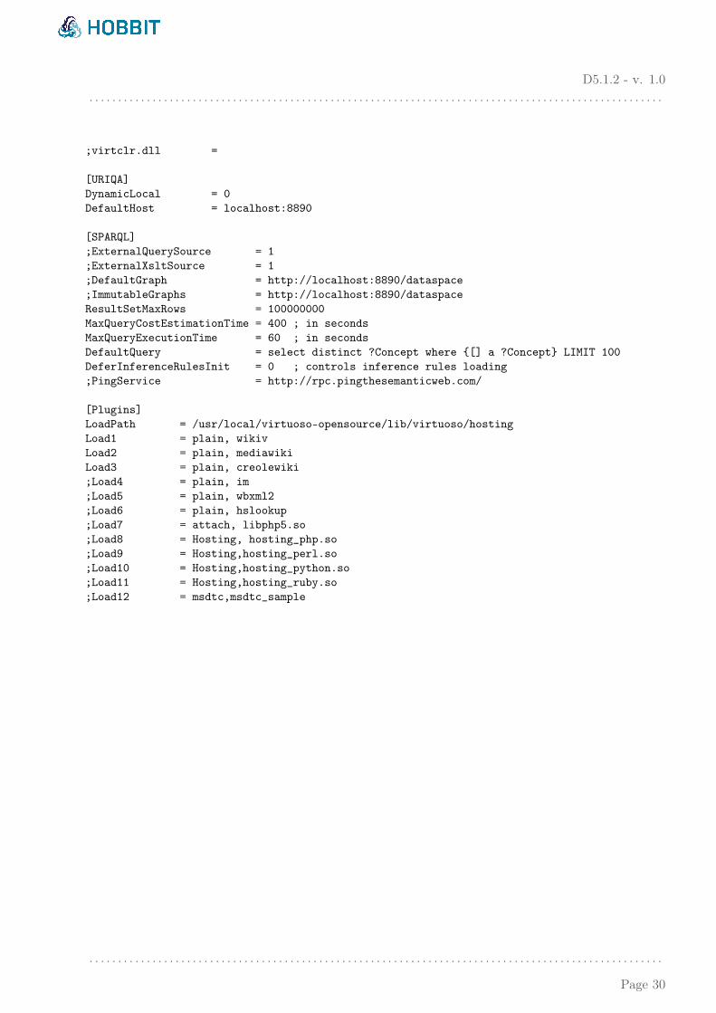
;virtclr.dll =

[URIQA]DynamicLocal = 0DefaultHost = localhost:8890

[SPARQL];ExternalQuerySource = 1;ExternalXsltSource = 1;DefaultGraph = http://localhost:8890/dataspace;ImmutableGraphs = http://localhost:8890/dataspaceResultSetMaxRows = 100000000MaxQueryCostEstimationTime = 400 ; in secondsMaxQueryExecutionTime = 60 ; in secondsDefaultQuery = select distinct ?Concept where {[] a ?Concept} LIMIT 100DeferInferenceRulesInit = 0 ; controls inference rules loading;PingService = http://rpc.pingthesemanticweb.com/

[Plugins]LoadPath = /usr/local/virtuoso-opensource/lib/virtuoso/hostingLoad1 = plain, wikivLoad2 = plain, mediawikiLoad3 = plain, creolewiki;Load4 = plain, im;Load5 = plain, wbxml2;Load6 = plain, hslookup;Load7 = attach, libphp5.so;Load8 = Hosting, hosting_php.so;Load9 = Hosting,hosting_perl.so;Load10 = Hosting,hosting_python.so;Load11 = Hosting,hosting_ruby.so;Load12 = msdtc,msdtc_sample

. . . . . . . . . . . . . . . . . . . . . . . . . . . . . . . . . . . . . . . . . . . . . . . . . . . . . . . . . . . . . . . . . . . . . . . . . . . . . . . . . . . . . . . . . . . . . . . . . . . .

Page 30