spread, volatility and volume relation in financial markets and market maker's profit...
TRANSCRIPT
1
Spread, volatility, and volume relationship in financial markets
and market maker’s profit optimization
Jack Sarkissian
Managing Member, Algostox Trading LLC
email: [email protected]
Abstract
We study the relationship between price spread, volatility and trading volume. We find that
spread forms as a result of interplay between order liquidity and order impact. When trading
volume is small adding more liquidity helps improve price accuracy and reduce spread, but
after some point additional liquidity begins to deteriorate price. The model allows to
connect the bid-ask spread and high-low bars to measurable microstructural parameters and
express their dependence on trading volume, volatility and time horizon. Using the
established relations, we address the operating spread optimization problem to maximize
the market-maker’s profit.
1. Introduction
When discussing security prices it is customary to describe them with single numbers. For example,
someone might say price of Citigroup Inc. (ticker “C”) on April 18, 2016 was $45.11. While good enough
for many uses, it is not entirely accurate. Single numbers can describe price only as referring to a particular
transaction, in which 𝑁 units of security are transferred from one party to another at a price $𝑋 each. Price
could be different a moment before or after the transaction, or if the transaction had different size, or if it
were executed on a different exchange. To be entirely accurate, one should specify these numerous details
when talking about security price.
Please cite as: J. Sarkissian, “Spread, Volatility, and Volume Relationship in Financial Markets and
Market Maker's Profit Optimization” (June 23, 2016). Available at SSRN:
http://ssrn.com/abstract=2799798
The enclosed materials are copyrighted materials. Federal law prohibits the unauthorized reproduction,
distribution or exhibition of the materials. Violations of copyright law will be prosecuted.

2
We will take this observation a step further. Technically speaking, other than at the time of transaction we
cannot say that price exists as a single number at all. Let us demonstrate this point. In financial markets
securities are normally bought and sold in an exchange, and the record of current orders is called an order
book. An example of order book is shown in Fig. 1. The order book shows how buyers (on the left side) are
willing to buy the security at a lower price and sellers (on the right side) are willing to sell it at a higher
price1. The trading parties wait in line for a matching order, and until that order arrives, the security does
not have a single price. Instead, there is a spectrum of prices, that could potentially represent the security
price.
Best candidates among them are the best bid 𝑠𝑏𝑖𝑑 and the best ask 𝑠𝑎𝑠𝑘 (marked green and red in Fig. 1).
The difference between the two is called the bid-ask spread:
Δ = 𝑠𝑎𝑠𝑘 − 𝑠𝑏𝑖𝑑, (1)
We can say that the security price is localized between the best bid and the best ask. When an order is
matched it disappears from order book and a transaction is recorded. Then the transaction price can be
referred to as the security price, but again, within the context of a particular transaction.
Buyers – bid Sellers - ask
Price Size Price Size
27.83 100 27.87 100
27.82 100 27.9 100
27.8 200 27.95 1000
27.79 600 28.15 300
27.78 100 28.2 400
Fig. 1. Sample order book. Buyers (on the left side) want to buy the security at a lower price and sellers
(on the right side) want to sell it at a higher price. Best bid is marked green, and best ask is marked red.
Often quotes in the order book come from market makers. Market makers are companies or desks within
companies that quote buy and sell prices of financial instruments for other market participants, while
providing commitment to buy and sell at the quoted prices. These firms profit from the bid-ask spread, and
1 Sometimes there might be no buyers or sellers, or neither buyers, nor sellers
3
spread management is crucial for them. As market makers, they compete for order execution and larger
turnover on the assets they quote.
Higher turnover is easily achieved by reducing the operating spread – the difference between market
maker’s own buy and sell quotes. However, reducing the operating spread also lowers income per trading
cycle2. To the contrary, increasing the operating spread increases income per cycle, but reduces turnover.
There is a tradeoff between spread and turnover, and the fundamental question is: what is the optimal
operating spread, that will maximize market maker’s profit from a given security?
Understanding spread behavior is important not only for market makers, but also for market users and
passive participants. It helps price discovery and allows them to save money by executing closer to the fair
price. Companies managing larger funds, particularly pension funds, can use it to price larger blocks of
securities. Understanding spread also provides tools for accurate risk management of securities with limited
liquidity.
Spread has a deep fundamental value. In order to demonstrate this, let us try to answer a question: what is
a measurement in finance and how is price measurement performed, [1-3]? If a number represents a valid
security price, then there must be parties in the market willing to transact the security at that price. In order
to test if the price is right, we must submit an order, for example a BUY order, at a discount price and keep
increasing the price until somebody wishes to sell at our price. Once our order executes, we can say that
price has been measured and the transaction price represents a valid security price. In fact, every
transaction in financial markets is an elementary act of price measurement.
How do we improve price accuracy? If we start with a small order it may not have enough weight to
represent price, so we may want to increase order size. It may work to a certain extent. However, at some
point the order will become so large that it will affect price. Other traders will see it and adjust their orders,
or our order will execute piercing multiple levels of order book – there are many ways how it can happen.
Even though the spread may still be low, price itself will become distorted. Apparently, there is an inherent
price uncertainty associated with the nature of price measurement. That uncertainty cannot be reduced and
is directly related to spread.
This quality has been pointed out in [4-9] to resemble the Heisenberg’s uncertainty principle in quantum
mechanics. In our earlier work [2] we showed that spread can be described as a quantum notion with
fluctuating coefficients, and that it obeys the statistics of quantum chaotic systems. In another work we
2 Market maker’s trading cycle consists of buying a security low from the current seller and selling it high to the
next available buyer (or shorting and covering it).

4
showed that, not only spread, but entire price evolution can be described with quantum chaotic framework
[1].
The most common approach is to obtain spread as a result of modeling processes in the order book. Once
order arrival, cancellation, and execution have been properly modeled, spread is obtained by direct
calculation [10,11]. Another approach is to obtain spread as the optimal value from market maker’s
perspective [12,13]. This approach allows to calculate spread from microstructural parameters, but also
depends on inventory held by market makers and their risk aversion level.
We are going to base our study on the considerations described in this section. Our goal is to express the
theoretical concept of spread as a bandgap in a lwo-level system [3,14] through observable and measurable
quantities. We are concerned with properties that have universal form, not depending on particulars of an
exchange system or company fundamentals. Naturally for financial industry, we are not looking for 100%
deterministic solutions. All relationships we find have statistical nature. But despite the statistical
dispersion, certain behavioral characteristics can be factored out to be applied practically.
Unlike our previous publications, here we will differentiate between bid-ask spread and high-low bars. Bid-
ask spread is related to the difference between the best bid and best offer, and is important to those who
want to provide liquidity based on its demand. High-low bars are related to fixed timeframe and are
important to those who simply want to update their quotes once in that timeframe while maintaining certain
execution level. As we shall see, there are substantial differences in behavior of the two quantities and that
is why we will differentiate them in this work.
Usually the designated market makers are subject to maintaining certain conditions, such as minimum
quotation time, maximum allowed spread or minimum turnover. We will overlook these details and will
focus on general framework. Firms and trading desks can include these additional conditions as they apply
to them.
And lastly, in order to maintain focus we will only consider the equity asset class. Same concepts can be
applied to other asset classes.
2. Basic relationship between spread, volatility and volume
Spread as price uncertainty
Many factors play role in spread formation, such as price uncertainty, transaction costs, holding premium,
etc [15-20]. Among them price uncertainty is the largest and most immediate. It is possible to evaluate the
5
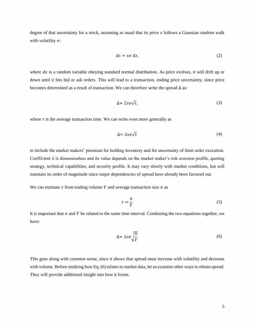
degree of that uncertainty for a stock, assuming as usual that its price 𝑠 follows a Gaussian random walk
with volatility 𝜎:
𝑑𝑠 = 𝑠𝜎 𝑑𝑧, (2)
where 𝑑𝑧 is a random variable obeying standard normal distribution. As price evolves, it will drift up or
down until it hits bid or ask orders. This will lead to a transaction, ending price uncertainty, since price
becomes determined as a result of transaction. We can therefore write the spread Δ as:
∆≈ 2𝑠𝜎√𝜏, (3)
where 𝜏 is the average transaction time. We can write even more generally as
∆= 𝜆𝑠𝜎√𝜏 (4)
to include the market makers’ premium for holding inventory and for uncertainty of limit order execution.
Coefficient 𝜆 is dimensionless and its value depends on the market maker’s risk aversion profile, quoting
strategy, technical capabilities, and security profile. It may vary slowly with market conditions, but will
maintain its order of magnitude since major dependencies of spread have already been factored out.
We can estimate 𝜏 from trading volume 𝑉 and average transaction size 𝑛 as
𝜏 =𝑛
𝑉 (5)
It is important that 𝜎 and 𝑉 be related to the same time interval. Combining the two equations together, we
have:
∆≈ 𝜆𝑠𝜎√𝑛
𝑉 (6)
This goes along with common sense, since it shows that spread must increase with volatility and decrease
with volume. Before studying how Eq. (6) relates to market data, let us examine other ways to obtain spread.
They will provide additional insight into how it forms.
6
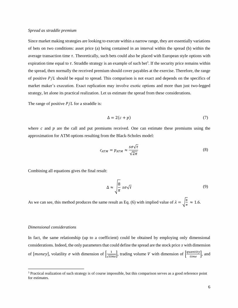
Spread as straddle premium
Since market making strategies are looking to execute within a narrow range, they are essentially variations
of bets on two conditions: asset price (a) being contained in an interval within the spread (b) within the
average transaction time 𝜏. Theoretically, such bets could also be placed with European style options with
expiration time equal to 𝜏. Straddle strategy is an example of such bet3. If the security price remains within
the spread, then normally the received premium should cover payables at the exercise. Therefore, the range
of positive 𝑃/𝐿 should be equal to spread. This comparison is not exact and depends on the specifics of
market maker’s execution. Exact replication may involve exotic options and more than just two-legged
strategy, let alone its practical realization. Let us estimate the spread from these considerations.
The range of positive 𝑃/𝐿 for a straddle is:
Δ = 2(𝑐 + 𝑝) (7)
where 𝑐 and 𝑝 are the call and put premiums received. One can estimate these premiums using the
approximation for ATM options resulting from the Black-Scholes model:
𝑐𝐴𝑇𝑀 = 𝑝𝐴𝑇𝑀 ≈𝑠𝜎√𝜏
√2𝜋 (8)
Combining all equations gives the final result:
Δ ≈ √8
𝜋 𝑠𝜎√𝜏 (9)
As we can see, this method produces the same result as Eq. (6) with implied value of 𝜆 = √8
𝜋 ≈ 1.6.
Dimensional considerations
In fact, the same relationship (up to a coefficient) could be obtained by employing only dimensional
considerations. Indeed, the only parameters that could define the spread are the stock price 𝑠 with dimension
of [𝑚𝑜𝑛𝑒𝑦], volatility 𝜎 with dimension of [1
√𝑡𝑖𝑚𝑒], trading volume 𝑉 with dimension of [
𝑞𝑢𝑎𝑛𝑡𝑖𝑡𝑦
𝑡𝑖𝑚𝑒], and
3 Practical realization of such strategy is of course impossible, but this comparison serves as a good reference point
for estimates.
7
average executing order size 𝑛 with dimension of [𝑞𝑢𝑎𝑛𝑡𝑖𝑡𝑦]. The only combination in which they
compose a spread with dimension of [𝑚𝑜𝑛𝑒𝑦] is
∆~𝑠 (𝑛𝜎2
𝑉)
𝑚
(10)
where 𝑚 is some power exponent. Realizing that under normal trading conditions spread must be
proportional to volatility, we figure 𝑚 =1
2:
∆= 𝜆𝑠 √𝑛𝜎2
𝑉 (11)
which is the same as Eq. (6). Market makers could set coefficient 𝜆 to any value they like. Smaller 𝜆 will
ensure more execution and bigger turnover, but will also result in larger residual risk from induced
inventory. Larger 𝜆 will ensure rare execution and smaller residual risk. One way to find a reasonable value
for coefficient 𝜆 is from market data. A market maker can then calibrate his 𝜆 relative to the market.
Relation to market data
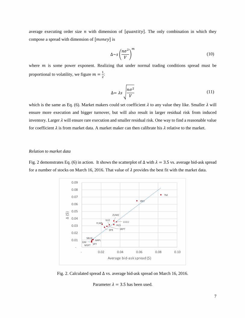
Fig. 2 demonstrates Eq. (6) in action. It shows the scatterplot of Δ with 𝜆 = 3.5 vs. average bid-ask spread
for a number of stocks on March 16, 2016. That value of 𝜆 provides the best fit with the market data.
Fig. 2. Calculated spread Δ vs. average bid-ask spread on March 16, 2016.
Parameter 𝜆 = 3.5 has been used.
AAPL
FLWS
GM
HLS
IRBT
LULU
MSFT
SBUX
SPR
SPY
SRPT
TM
VLO
ZUMZ
-
0.01
0.02
0.03
0.04
0.05
0.06
0.07
0.08
0.09
- 0.02 0.04 0.06 0.08 0.10
Δ (
$)
Average bid-ask spread ($)

8
Figs. 3a-d show how Eq. (6) works for spread dynamics. It displays calibrated Δ and average bid-ask spread
in the period March 1-16, 2016 for AMZN (Amazon.com, Inc.) and LULU (Lululemon Athletica inc.).
(a) (b)
Fig. 3a-b. Dynamics and correlation of calibrated Δ and average bid-ask spread
during the period of March 1-16, 2016 for AMZN.
(c) (d)
Fig. 3c-d. Dynamics and correlation of calibrated Δ and average bid-ask spread
during the period of March 1-16, 2016 for LULU.
-
0.1
0.2
0.3
0.4
0.5
0.6
1 6 11 16
Day
AMZN
Bid-ask spread Δ
-
0.1
0.2
0.3
0.4
0.5
0.6
- 0.1 0.2 0.3 0.4 0.5 0.6
Δ($
)Bid-ask spread ($)
AMZN
-
0.01
0.02
0.03
0.04
0.05
1 6 11 16
Day
LULU
Bid-ask spread Δ
-
0.01
0.02
0.03
0.04
0.05
- 0.01 0.02 0.03 0.04 0.05
Δ($
)
Bid-ask spread ($)
LULU

9
Thus, we established that spread, volatility, and trading volume are not independent variables and are
connected through Eq. (6). We also estimated the market’s implied value for 𝜆 to be around 𝜆 = 3.5.
Relation Eq. (6) describes spread for various securities and captures its dynamics. It is important that no
assumptions about the security, company, or market structure, other than that the security price follows a
Wiener process, were made in deriving it.
3. Microscopic theory
Overview of quantum coupled-wave model
Eq. (6) says that spread must always decrease with volume. According to market data this is only true to a
certain extent: when volume is large spread starts growing with volume, (see Figs. 11-13). In order to obtain
the general relationship for spread, we need to use a model that deals with it as an intrinsic property of
financial instruments and that captures its statistical properties.
Such model was developed in our earlier paper [2]. In that paper we proposed the idea that security prices
can be described as eigenvalues of price operator acting on probability amplitude, so that:
�̂�𝜓𝑛 = 𝑠𝑛𝜓𝑛 (12)
and 𝑝𝑛 = |𝜓𝑛|2 (13)
Matrix elements of the price operator fluctuate in time, due to which its eigenvalues and eigenfunctions
acquire random properties:
�̂�(𝑡 + 𝛿𝑡) = �̂�(𝑡) + 𝛿�̂�(𝑡) (14)
Here we will slightly modify it compared to [2] to build it for transfer between high and low levels, realizing
that bid and ask are also a special case of high-low at the time scale equal to 𝜏. For a two-level system
Eq. (12) takes the following form:
𝜓 = (𝜓ℎ𝑖𝑔ℎ
𝜓𝑙𝑜𝑤) and (
𝑠11 𝑠12
𝑠12∗ 𝑠22
) (𝜓ℎ𝑖𝑔ℎ
𝜓𝑙𝑜𝑤) = 𝑠ℎ𝑖𝑔ℎ/𝑙𝑜𝑤 (
𝜓ℎ𝑖𝑔ℎ
𝜓𝑙𝑜𝑤) (15)

10
Given this, the high and low prices can be obtained as
𝑠ℎ𝑖𝑔ℎ = 𝑠𝑚𝑖𝑑 +ℎ
2 and 𝑠𝑙𝑜𝑤 = 𝑠𝑚𝑖𝑑 −
ℎ
2 (16a)
𝑠𝑚𝑖𝑑 =
𝑠11 + 𝑠22
2=
𝑠𝑙𝑜𝑤 + 𝑠ℎ𝑖𝑔ℎ
2 (mid − price) (16b)
ℎ = √(𝑠11 − 𝑠22)2 + 4|𝑠12|2 (bar height or spread) (16c)
Matrix elements 𝑠𝑖𝑘 of price operator are then parametrized to include fluctuations:
𝑠11(𝑡 + 𝑑𝑡) = 𝑠𝑙𝑎𝑠𝑡(𝑡) + 𝑠𝑙𝑎𝑠𝑡(𝑡) 𝜎𝑑𝑧 +
𝜉
2 (17a)
𝑠22(𝑡 + 𝑑𝑡) = 𝑠𝑙𝑎𝑠𝑡(𝑡) + 𝑠𝑙𝑎𝑠𝑡(𝑡) 𝜎𝑑𝑧 −
𝜉
2 (17b)
𝑠12(𝑡 + 𝑑𝑡) =𝜅
2 (17c)
where 𝑑𝑧 ∼ 𝑁(0,1), 𝜉~𝑁(𝜉0, 𝜉1) and 𝜅~𝑁(𝜅0, 𝜅1). In such setup the mid-price, the bar height and last
price are given by equations
𝑠𝑚𝑖𝑑(𝑡 + 𝑑𝑡) = 𝑠𝑙𝑎𝑠𝑡(𝑡) + 𝑠𝑙𝑎𝑠𝑡(𝑡) 𝜎𝑑𝑧 (18a)
ℎ = √𝜉2 + 𝜅2 (18b)
𝑠𝑙𝑎𝑠𝑡(𝑡 + 𝑑𝑡)~𝑢𝑛𝑖𝑓(𝑠𝑙𝑜𝑤 , 𝑠ℎ𝑖𝑔ℎ) (18c)
At each step the next mid-price takes a value normally distributed around the last price. The high and low
levels take values ℎ/2 above and below the mid-price. Then the next last price takes a random value
uniformly distributed between the high and low levels. Price chart that can be generated by the model,
Eqs. (18a-c) is shown in Fig. 4. Volatility of prices (as referring to last prices) is equal
𝜂 = √𝑠2𝜎2𝑑𝑡 + 𝛼ℎ2
4 (19)

11
where 𝛼 is a coefficient that corresponds to distribution of 𝑠𝑙𝑎𝑠𝑡 in Eq. (18c)4, and we used notation 𝑠 for
𝑠𝑙𝑎𝑠𝑡. Rather than considering bars as rigid boundaries beyond which price cannot extend, it is possible to
think of them as the characteristic distribution width of the last price around mid-price. For example, that
distribution can be normal with half the bar height as its standard deviation:
𝑠𝑙𝑎𝑠𝑡(𝑡 + 𝑑𝑡)~𝑁 (𝑠𝑚𝑖𝑑 ,ℎ
2) (20)
In this case volatility is:
𝜂 = √𝑠2𝜎2𝑑𝑡 +ℎ2
4 (21)
Fig. 4. Price chart generated by coupled-wave model. At each step the next mid-price takes a value
normally distributed around the last price. The high and low levels take equally spaced values above and
below the mid-price. Then the next last price takes a random value uniformly distributed between the high
and low levels.
Bars described by Eq. (18b) behave as quantum-chaotic quantities [2], whose statistics matches the
observed statistics quite well both on bid-ask micro-level and on bar data level, see Figs. 5a, 5b.
4 Statistics of trades inside the high-low range can be different for different time scales, which will result in different
𝛼. For example, trades execute at bid or ask levels but not in the middle, but as we move up in time horizon, trades
become more frequent in the middle of the high-low range and scarce at its edges.
0
20
40
60
80
100
120
0 20 40 60 80 100
time
high low price

12
Fig. 5a. Calibration of coupled-wave model to bid-ask data for AAPL and AMZN, [2]
Fig 5b. Calibration of coupled-wave model to bar data for AAPL and AMZN, [2]
Evolution of probability amplitude 𝜓 is described by equation [1,2]:
𝑖𝜏0𝑠𝜕𝜓
𝜕𝑡= �̂�𝜓 (22)
or in an open form
𝑖𝜏0𝑠𝑑𝜓ℎ𝑖𝑔ℎ
𝑑𝑡= 𝑠11𝜓ℎ𝑖𝑔ℎ + 𝑠12𝜓𝑙𝑜𝑤 (23a)
𝑖𝜏0𝑠𝑑𝜓𝑙𝑜𝑤
𝑑𝑡= 𝑠12
∗ 𝜓ℎ𝑖𝑔ℎ + 𝑠22𝜓𝑙𝑜𝑤 (23b)
AAPL AMZN
AAPL AMZN
13
Here 𝜏0 is some constant with dimension of time. For constant coefficients this system of equations has the
following solution, expressed through model parameters ℎ, 𝜉, and 𝜅 [2]:
𝜓ℎ𝑖𝑔ℎ(𝑡) = 𝑒−𝑖𝑠𝑚𝑖𝑑𝑡 {[𝑐𝑜𝑠 (ℎ
2𝜏0𝑠𝑡) − 𝑖
𝜉
ℎ𝑠𝑖𝑛 (
ℎ
2𝜏0𝑠𝑡)] 𝜓ℎ𝑖𝑔ℎ(0) − 𝑖
𝜅
ℎ𝑠𝑖𝑛 (
ℎ
2𝜏0𝑠𝑡) 𝜓𝑙𝑜𝑤(0)} (24a)
𝜓𝑙𝑜𝑤(𝑡) = 𝑒−𝑖𝑠𝑚𝑖𝑑𝑡 {−𝑖𝜅
ℎ𝑠𝑖𝑛 (
ℎ
2𝜏0𝑠𝑡) 𝜓ℎ𝑖𝑔ℎ(0) + [𝑐𝑜𝑠 (
ℎ
2𝜏0𝑠𝑡) + 𝑖
𝜉
ℎ𝑠𝑖𝑛 (
ℎ
2𝜏0𝑠𝑡)] 𝜓𝑙𝑜𝑤(0)} (24b)
Since in fact coefficients ijs fluctuate, solution has to be applied numerically in small time steps, during
which price operator elements ijs can be considered constant.
General relation for spread
Coupled-wave model contains three dimensions of uncertainty: (a) uncertainty of the mid-price, Eq. (18a),
(b) uncertainty of bar size, Eq. (18b), and uncertainty of price within the bar, Eq. (18c). The first two
elements accumulate over time, while the uncertainty of price within the bar is present from the beginning.
Spread must cover these risks over the liquidation period 𝜏. Scaling these risk components each according
to its risk-aversion level, we can compose the spread to be
Δ = √(𝜌ℎ)2
4+ (𝜆𝜂)2 (25)
where in this case 𝜂 = √𝑠2𝜎2𝜏 +𝜌2
𝜆2
ℎ2
4. The initial uncertainty is
ℎ
2 up and down, and over time 𝜏, it accrues
𝑠𝜎√𝜏 and another half-bar ℎ
2. To be accurate, we should have used different ℎ for the initial and subsequent
bars, but for our purposes we will be using characteristic values. Eventually, we have
Δ = √(𝜌ℎ)2
2+ (𝜆𝑠𝜎)2𝜏 (26)
Let us link all components to observable quantities. The second term under the square root is the already
familiar element associated with price uncertainty due to finite liquidation time. It is essentially the price
that a buy-side trader must pay in order to access immediate liquidity. We can call it the liquidity price.
14
Bar size ℎ determines oscillation frequency in Eqs. (24a,b). Oscillation period corresponds to double the
average transaction time 2𝜏, in which the security is transferred back and forth in a full cycle. We must
therefore have
ℎ𝜏
2𝑠𝜏0≈ 𝜋 (27)
and as a result:
ℎ ≈ 2𝜋𝜏0
𝑠
𝜏 (28)
Noting that 𝑠
𝜏 is the amount of money per share traded in a transaction, we come to conclusion that ℎ
represents money flow and characterizes the degree of price impact caused by that flow. We will call it the
impact price.
Within ℎ, parameter 𝜅 is associated with securities transfer between the “high” and “low” levels, and
parameter 𝜉 is associated with the intensity of that transfer. This can be verified by direct modeling of
Eqs. (24a,b) and varying 𝜉 and 𝜅, particularly using combinations 𝜉 = 0, 𝜅 ≠ 0 and 𝜅 = 0, 𝜉 ≠ 0.
Combining Eqs. (5, 26, 28), we have the final result for the spread:
Δ = √(𝜆𝑠𝜎√𝜏)2
+ 2 (𝜌𝜋𝑠𝜏0
𝜏)
2
= √𝜆2𝑠2𝜎2𝑛
𝑉+ 2𝜌2 (
𝜋𝑠𝜏0
𝑛)
2
𝑉2 (29)
We can shape up this equation writing it in a simpler dimensionless format:
𝛿(𝑣) = √𝑎
𝑣+ 𝑣2 (30)
where 𝛿 =Δ
𝑠, 𝑎 = √2𝜌𝜆2𝜎2(𝜋𝜏0), 𝑣 =
𝑉
𝑉0, and 𝑉0 =
1
√2𝜌
𝑛
𝜋𝜏0.
Eq. (30) relates the spread to microstructural parameters and is more general than Eq. (6). We see that
spread can have two regimes with different characteristic behavior. When volume is small, such that
𝑣 ≪ √𝑎3
, the liquidity price contribution prevails over impact price contribution and spread exhibits the
already familiar behavior: δ(𝑣)~1
√𝑣 . This regime is shown in Fig. 6a, where we can see how adding more
flow to trading reduces the spread and helps improve price. This is valid as long as volume is not large
enough to affect price. When 𝑣 ≫ √𝑎3
, so that cash value of executing orders becomes larger than the
liquidity price, these orders begin to impair price measurement and spread starts to grow linearly with
volume: δ(𝑣)~𝑣. This regime is shown in Fig. 6b.

15
(a) (b)
Fig. 6. Interplay between liquidity price and impact price: (a) impact is small and adding more liquidity
improves price accuracy, (b) impact is so large that it impairs price.
Minimum spread and price uncertainty
Due to the functional form of Eq. (30), 𝛿(𝑣) does not reach zero. It reaches minimum at 𝑣𝑚𝑖𝑛 = √𝑎
2
3, and
its minimum value is equal to 𝛿𝑚𝑖𝑛 = √3 𝑣𝑚𝑖𝑛. For every spread 𝛿 > 𝛿𝑚𝑖𝑛 there are two values of 𝑣 that
correspond to it.
Time scaling of spread
What happens if a desk quotes prices based on some time scale and wants to change to another time scale5.
What is the relationship between high-low bars at different time scales? How do we transition from bid-ask
spread to bars, or between the bars of different time scales?
If we were to quote at a different time scale with the same risk aversion, we would just use the volatility
related to that time scale in Eq. (25) and add it to the initial uncertainty, represented by the initial bar:
Δ𝑇 = √𝜌2ℎ𝜏
2
4+ 𝜆2𝜂𝜏
2𝑇
𝜏 (31)
5 Some desks do tick-based quoting, which is tied to market events, while others do bar-based quoting refreshing their
quotes after certain time. But even the bar-based quoters require this transition since they normally randomize their
time horizon.
Liq
uid
ity
pri
ce
𝑠𝑎𝑠𝑘
𝑠𝑎𝑠𝑘′
Impact price
𝑠𝑏𝑖𝑑
𝑡
𝑠𝑏𝑖𝑑′
Liq
uid
ity
pri
ce
𝑠𝑎𝑠𝑘
Impact price
𝑠𝑎𝑠𝑘′
𝑠𝑏𝑖𝑑 𝑠𝑏𝑖𝑑′
𝑡

16
where indexes now indicate the reference time, and 𝑇 ≥ 𝜏. Expressing Δ𝑇2 through the parameters related
to reference time 𝑇1, we get
Δ𝑇2 = Δ𝑇1 √1 + 𝜆2𝜂𝑇
21
Δ𝑇2
1
(𝑇2
𝑇1− 1) (32)
Particularly, Δ𝑇 is related to bid-ask spread Δ𝜏 = √𝜌2ℎ𝜏2
4+ 𝜆2𝜂𝜏
2 through:
Δ𝑇 = Δ𝜏 √1 + 𝜆2𝜂𝜏
2
Δ𝜏2
(𝑇
𝜏− 1) (33)
This agrees with the result obtained in our other work [1] (Eq. (43) in it). Equations are mapped to each
other with the following substitutions:
Δ𝜏 ↔ 𝑤Δt
𝜆𝜂𝜏 ↔ 𝛽𝜖
𝜏 ↔ Δ𝑡
Some spread curves calibrated to average intraday minute bars, observed on March 16, 2016, and average
daily bars are shown in Figs. (7a and 7b).
Fig. 7a. Spread curves calibrated to average 1-minute intraday (left) and daily (right) bars for ticker LULU
0.0%
0.2%
0.4%
0.6%
0.8%
1.0%
- 20 40 60
Spre
ad
Time (min)
LULU
High-low δ(T)
0%
10%
20%
30%
40%
- 20 40 60
Spre
ad
Time (days)
LULU
High-low δ(T)

17
Fig. 7b. Spread curves calibrated to 1-minute intraday (left) and daily (right) bars for ticker AMZN
Comparison to classical theory
According to classical theory volatility scales as square root of time6:
𝜂𝑇2= √
𝑇2
𝑇1𝜂𝑇1
(34)
This implies that price accuracy can be indefinitely improved by reducing measurement time. This is not
true in real markets, as was discussed in Introduction section, and Eq. (33) does not allow it. Only over long
time horizon volatility prevails and the effect of the initial spread disappears, leading to regular square root-
like behavior:
Δ𝑇2≈ √
𝑇2
𝑇1Δ𝑇1
(35)
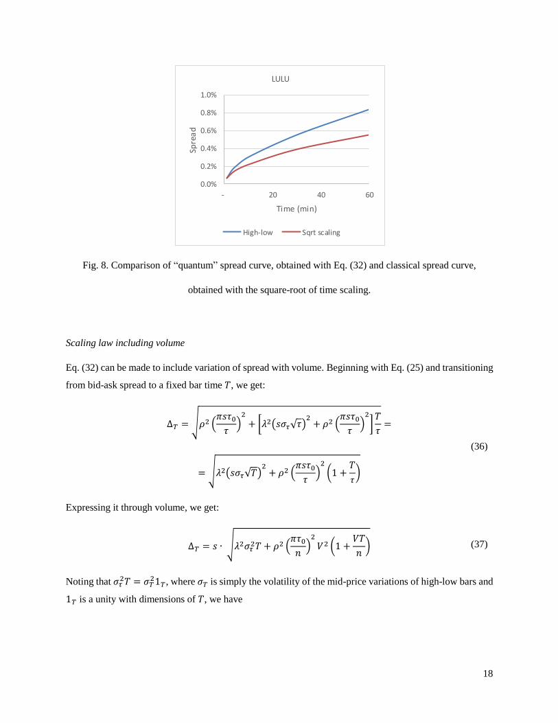
To see the difference visually, we can take the spread curve of the LULU stock. If a 1-minute high-low bar
was scaled forward to 60 minutes with Eq. (35), the result would be 0.55%, which about 35% off the real
value.
6 Strictly speaking, this relates to volatility of returns. However, since return 𝑟 =
𝑠
𝑠0− 1, the relation is the same for
small price deviations discussed here.
0.0%
0.2%
0.4%
0.6%
0.8%
1.0%
- 20 40 60
Spre
ad
Time (min)
AMZN
High-low δ(T)
0%
10%
20%
30%
- 20 40 60
Spre
ad
Time (days)
AMZN
High-low δ(T)
18
Fig. 8. Comparison of “quantum” spread curve, obtained with Eq. (32) and classical spread curve,
obtained with the square-root of time scaling.
Scaling law including volume
Eq. (32) can be made to include variation of spread with volume. Beginning with Eq. (25) and transitioning
from bid-ask spread to a fixed bar time 𝑇, we get:
Δ𝑇 = √𝜌2 (𝜋𝑠𝜏0
𝜏)
2
+ [𝜆2(𝑠𝜎𝜏√𝜏)2
+ 𝜌2 (𝜋𝑠𝜏0
𝜏)
2
]𝑇
𝜏=
= √𝜆2(𝑠𝜎𝜏√𝑇)2
+ 𝜌2 (𝜋𝑠𝜏0
𝜏)
2
(1 +𝑇
𝜏)
(36)
Expressing it through volume, we get:
Δ𝑇 = 𝑠 ∙ √𝜆2𝜎𝜏2𝑇 + 𝜌2 (
𝜋𝜏0
𝑛)
2
𝑉2 (1 +𝑉𝑇
𝑛) (37)
Noting that 𝜎𝜏2𝑇 = 𝜎𝑇
21𝑇, where 𝜎𝑇 is simply the volatility of the mid-price variations of high-low bars and
1𝑇 is a unity with dimensions of 𝑇, we have
0.0%
0.2%
0.4%
0.6%
0.8%
1.0%
- 20 40 60Sp
rea
d
Time (min)
LULU
High-low Sqrt scaling

19
Δ𝑇(𝑉) = 𝑠 ∙ √𝜆2𝜎𝑇21𝑇 + 𝜌2 (
𝜋𝜏0
𝑛)
2
𝑉2 + 𝜌2(𝜋𝜏0)2𝑇
𝑛3𝑉3 (38)
or in dimensionless format:
𝛿𝑇(𝑣) = √𝜆2𝜎𝑇21𝑇 +
𝑣2
2+
𝑇
23/2 𝜌𝜋𝜏0
𝑣3 (39)
We see that high-low bars depend on volume completely differently than bid-ask spread. Unlike 𝛿𝜏 the 𝜎
term for 𝛿𝑇 does not depend on volume, and along with 𝑣 there is now a 𝑣3/2 behavior, which prevails at
large time horizons. Unlike 𝛿𝜏, which has a minimum, 𝛿𝑇 starts with its minimum value at 𝑣𝑇 = 0 and only
increases with volume. The differences can be seen in Fig. (9) showing characteristic 𝛿𝜏(𝑣) and 𝛿𝑇(𝑣)
behavior.
Fig. 9. Qualitative difference in behavior between (a) bid-ask spread and (b) high-low bars.
Risk aversion level
Eqs. (29 and 38) provide a good reference, but not yet the final answers to spread modeling. One reason is
that statistics of trades inside the high-low range can be different for data at different time scales, which
will result in different 𝛼 in Eq. (19). For example, trades execute at bid or ask levels, but not inside the
spread. Same trades can be more evenly distributed between the high and low levels on minute time scale.
0.00%
0.02%
0.04%
0.06%
0.08%
0.10%
0 100,000 200,000 300,000 400,000 500,000
Volume
spread bars
20
Lastly, in daily data trades usually occur around the center of high-low interval rather than by its edges.
Transitions between time scales must include variation of 𝛼 with time scale.
Another point is that risk aversion level depends on numerous factors. For example, market makers would
usually ask a bigger premium to quote at smaller time scale than at large time scale. Additionally, they will
generally set larger spreads at market opening since they are unsure about market consensus regarding
prices. They will subsequently lower spreads once such consensus is established. Market makers will also
increase spreads closer to the end of the day in order to prepare for longer holding timeframe (until market
open) or to reduce chances of carrying overnight positions.
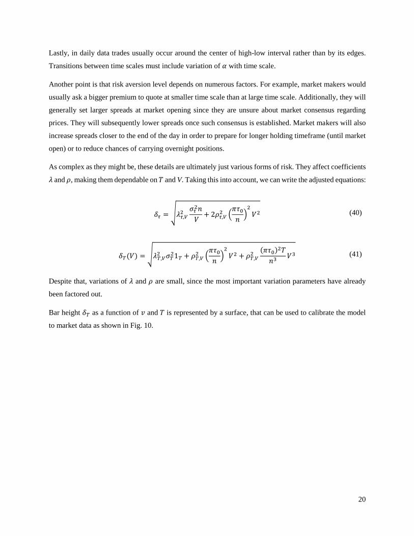
As complex as they might be, these details are ultimately just various forms of risk. They affect coefficients
𝜆 and 𝜌, making them dependable on 𝑇 and V. Taking this into account, we can write the adjusted equations:
𝛿𝜏 = √𝜆𝜏,𝑉2
𝜎𝜏2𝑛
𝑉+ 2𝜌𝜏,𝑉
2 (𝜋𝜏0
𝑛)
2
𝑉2 (40)
𝛿𝑇(𝑉) = √𝜆𝑇,𝑉2 𝜎𝑇
21𝑇 + 𝜌𝑇,𝑉2 (
𝜋𝜏0
𝑛)
2
𝑉2 + 𝜌𝑇,𝑉2
(𝜋𝜏0)2𝑇
𝑛3𝑉3 (41)
Despite that, variations of 𝜆 and 𝜌 are small, since the most important variation parameters have already
been factored out.
Bar height 𝛿𝑇 as a function of 𝑣 and 𝑇 is represented by a surface, that can be used to calibrate the model
to market data as shown in Fig. 10.

21
Fig. 10. Spread surface for AMZN.
It is natural to use 𝜆 and 𝜌 as control parameters allowing to gauge execution rate. Numerical connection
between the two will be established in the next section.
Connection with market data
As an example Figs. 11-13 present spread-volume data based on bid-ask spread, 1-minute intraday high-
low bars, and daily high-low bars for AMZN and LULU. The spread-volume curves correspond to
execution rate levels of 90%. They were obtained by taking the scatterplot of spread vs. volume, splitting
it into volume buckets, and calculating the 90-th percentile across the spread for each bucket. Values for 𝑛
and 𝜎𝜏 were measured directly from trading flow data. What was left after that is only to select 𝜏0 and
calibrate 𝜆 and 𝜌. In order to make judgement of statistical significance easier, we supplement main plots
with trade frequency using an additional vertical axis.
The model works pretty well for daily high-low data. It gets more complex for bid-ask and 1-minute high-
low data. One can notice how the model works better on LULU than AMZN. This is because coupled-wave
model assumes only two price levels at each step, and LULU has much more distinct levels than AMZN.
This is apparent from trade frequency data, so LULU is better approximated by a two-level system. In order
to describe AMZN more accurately, a multi-level model has to be used.
We can also see that 1-minute high-low bars do not start with a finite value, but grow from almost zero
values (daily bars are fine in that respect). This is where the already mentioned effect of change in trade
1
200
400600
8001000
0.0%
2.0%
4.0%
6.0%
8.0%
10.0%
12.0%
Tim
e (m
in)
δ
Volume (#/min)
22
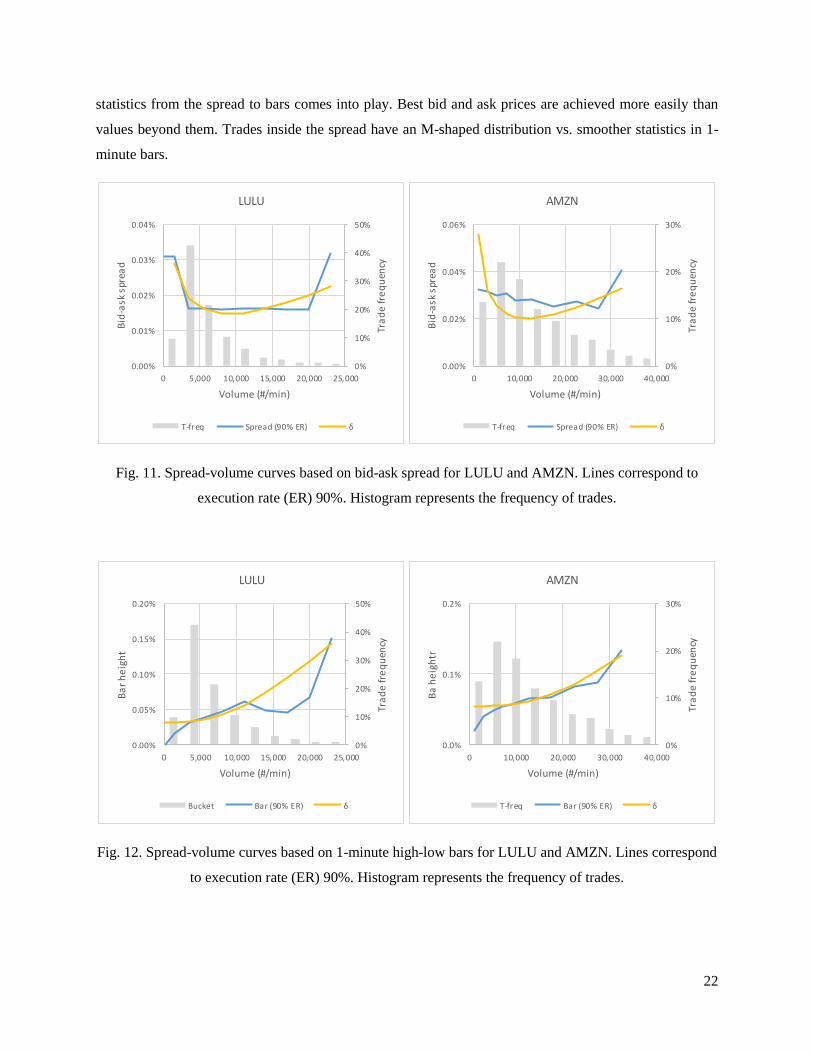
statistics from the spread to bars comes into play. Best bid and ask prices are achieved more easily than
values beyond them. Trades inside the spread have an M-shaped distribution vs. smoother statistics in 1-
minute bars.
Fig. 11. Spread-volume curves based on bid-ask spread for LULU and AMZN. Lines correspond to
execution rate (ER) 90%. Histogram represents the frequency of trades.
Fig. 12. Spread-volume curves based on 1-minute high-low bars for LULU and AMZN. Lines correspond
to execution rate (ER) 90%. Histogram represents the frequency of trades.
0%
10%
20%
30%
40%
50%
0.00%
0.01%
0.02%
0.03%
0.04%
0 5,000 10,000 15,000 20,000 25,000Tr
ad
e fr
eq
uen
cy
Bid
-ask
spr
ead
Volume (#/min)
LULU
T-freq Spread (90% ER) δ
0%
10%
20%
30%
0.00%
0.02%
0.04%
0.06%
0 10,000 20,000 30,000 40,000
Tra
de
fre
qu
ency
Bid
-ask
spr
ead
Volume (#/min)
AMZN
T-freq Spread (90% ER) δ
0%
10%
20%
30%
40%
50%
0.00%
0.05%
0.10%
0.15%
0.20%
0 5,000 10,000 15,000 20,000 25,000
Tra
de
fre
qu
ency
Ba
r h
eig
ht
Volume (#/min)
LULU
Bucket Bar (90% ER) δ
0%
10%
20%
30%
0.0%
0.1%
0.2%
0 10,000 20,000 30,000 40,000
Tra
de
fre
qu
ency
Ba
he
igh
tr
Volume (#/min)
AMZN
T-freq Bar (90% ER) δ

23
Fig. 13. Spread-volume curves based on daily high-low bars for LULU and AMZN. Lines correspond to
execution rate (ER) 90%. Histogram represents the frequency of trading volume.
4. Spread control and market maker’s profit optimization
Armed with functional dependence 𝛿(𝑣) we can now approach the problem of spread control and
optimization. Market maker’s P/L consists of two major components: spread revenue and inventory P/L.
Spread revenue comes from executing buy and sell orders and keeping the price difference. Inventory P/L
is the result of mark-to-market of the inventory held on market maker’s book between buying and selling.
Since market makers essentially bet against price direction, that mark-to-market usually produces a loss.
While inventory P/L is an extremely important component, that can substantially distort the net P/L profile,
it has a substantially different nature from spread revenue and firms have various approaches dealing with
it. Here we will focus on the spread revenue part.
If market maker executes bid and ask quotes with execution rate 𝑟 on a security that trades at volume 𝑣,
then the market maker’s turnover is 𝑟𝑣. Execution costs and rebates 𝛼 are usually proportional to turnover,
so if quoted spread is 𝛿, earnings per round trip are 𝛿 − 𝛼. The spread P/L over the period is then equal
𝑃/𝐿 = 0.5 𝑟𝑣(𝛿 − 𝛼) (42)
Here 𝑟 is a function of 𝛿, and factor 0.5 reflects the fact that the security has to be bought and sold. An
example of the resulting curve is shown in Fig. 14. The question is: what is the optimal operating spread
that maximizes P/L? How should it be adjusted depending on current volume in order to guarantee
maximum P/L? And are there conditions under which trading should be halted?
0%
10%
20%
30%
40%
0%
2%
4%
6%
8%
0 2 4 6 8 10
Tra
de
fre
qu
ency
Ba
r h
eig
ht
Volume (mln #/day)
LULU
T-freq Bar (90% ER) δ
0%
10%
20%
30%
40%
0%
2%
4%
6%
8%
0 5 10 15
Tra
de
fre
qu
ency
Ba
r h
eig
ht
Volume (mln #/day)
AMZN
T-freq Bar (90% ER) δ
24
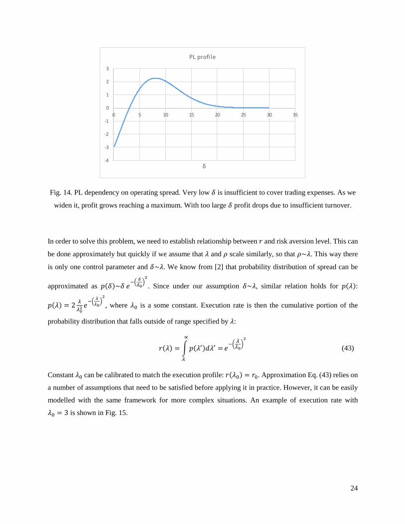
Fig. 14. PL dependency on operating spread. Very low 𝛿 is insufficient to cover trading expenses. As we
widen it, profit grows reaching a maximum. With too large 𝛿 profit drops due to insufficient turnover.
In order to solve this problem, we need to establish relationship between 𝑟 and risk aversion level. This can
be done approximately but quickly if we assume that 𝜆 and 𝜌 scale similarly, so that 𝜌~𝜆. This way there
is only one control parameter and 𝛿~𝜆. We know from [2] that probability distribution of spread can be
approximated as 𝑝(𝛿)~𝛿 𝑒−(
𝛿
𝛿0)
2
. Since under our assumption 𝛿~𝜆, similar relation holds for 𝑝(𝜆):
𝑝(𝜆) = 2𝜆
𝜆02 𝑒
−(𝜆
𝜆0)
2
, where 𝜆0 is a some constant. Execution rate is then the cumulative portion of the
probability distribution that falls outside of range specified by 𝜆:
𝑟(𝜆) = ∫ 𝑝(𝜆′)𝑑𝜆′ =
∝
𝜆
𝑒−(
𝜆𝜆0
)2
(43)
Constant 𝜆0 can be calibrated to match the execution profile: 𝑟(𝜆0) = 𝑟0. Approximation Eq. (43) relies on
a number of assumptions that need to be satisfied before applying it in practice. However, it can be easily
modelled with the same framework for more complex situations. An example of execution rate with
𝜆0 = 3 is shown in Fig. 15.
-4
-3
-2
-1
0
1
2
3
0 5 10 15 20 25 30 35
δ
PL profile

25
Fig. 15. Execution rate dependency on 𝜆.
(a) (b)
Fig. 16. 𝜆 and 𝑟 dependency on trading volume for bid-ask quoting.
Optimal execution rate can then be found from solving the following equation with respect to 𝑟:
𝛿 − 𝛼 + 𝑟𝜕𝛿
𝜕𝑟= 0 (44)
0%
20%
40%
60%
80%
100%
0 2 4 6 8 10
Exec
uti
on
ra
te
λ
0
0.5
1
1.5
2
2.5
3
0 2 4 6 8 10
v
Optimal λ
0%
10%
20%
30%
40%
50%
60%
70%
0 2 4 6 8 10
v
Optimal execution rate
26
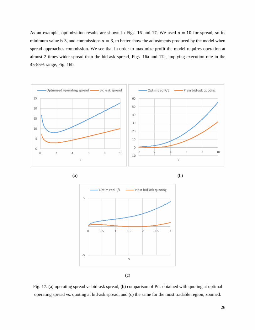
As an example, optimization results are shown in Figs. 16 and 17. We used 𝑎 = 10 for spread, so its
minimum value is 3, and commissions 𝛼 = 3, to better show the adjustments produced by the model when
spread approaches commission. We see that in order to maximize profit the model requires operation at
almost 2 times wider spread than the bid-ask spread, Figs. 16a and 17a, implying execution rate in the
45-55% range, Fig. 16b.
(a) (b)
(c)
Fig. 17. (a) operating spread vs bid-ask spread, (b) comparison of P/L obtained with quoting at optimal
operating spread vs. quoting at bid-ask spread, and (c) the same for the most tradable region, zoomed.
0
5
10
15
20
25
0 2 4 6 8 10
v
Optimized operating spread Bid-ask spread
-10
0
10
20
30
40
50
60
0 2 4 6 8 10
v
Optimized P/L Plain bid-ask quoting
-5
5
0 0.5 1 1.5 2 2.5 3
v
Optimized P/L Plain bid-ask quoting

27
Behavior suggested by the model is opposite to that of buy-side. It proposes a more aggressive quoting (a)
when trading volume is low and liquidity is limited, which is when market makers are most needed, and
(b) when volume is large, which usually happens at times of large volatility, when the buy-side isn’t sure
about prices. Execution rate has to be lowered when bid-ask spread is around its minimum values, which
helps to reduce the effect of the commissions. Optimized profit is shown in Figs. 17b and zoomed in
Fig. 17c, versus the P/L made with plain bid-ask spread quoting. Similar charts are shown for bar-based
quoting in Figs. 18, and 19.
Fig. 18. 𝜆 and 𝑟 dependency on trading volume for bar quoting.
(a) (b)
0
0.5
1
1.5
2
2.5
3
0 2 4 6 8 10
v
Optimal λ
0%
10%
20%
30%
40%
50%
60%
70%
0 2 4 6 8 10
v
Optimal execution rate
0
20
40
60
80
0 2 4 6 8 10
v
Optimized operating spread High-low bars
0
50
100
150
200
0 2 4 6 8 10
v
Optimized P/L Plain bar quoting
28
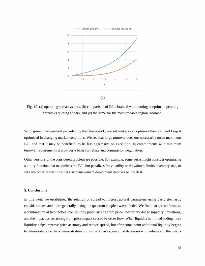
(c)
Fig. 19. (a) operating spread vs bars, (b) comparison of P/L obtained with quoting at optimal operating
spread vs quoting at bars, and (c) the same for the most tradable region, zoomed.
With spread management provided by this framework, market makers can optimize their P/L and keep it
optimized in changing market conditions. We see that large turnover does not necessarily mean maximum
P/L, and that it may be beneficial to be less aggressive on execution. In commitments with minimum
turnover requirements it provides a basis for rebate and commission negotiation.
Other versions of the considered problem are possible. For example, some desks might consider optimizing
a utility function that maximizes the P/L, but penalizes for volatility or drawdown, limits inventory size, or
sets any other restrictions that risk management department imposes on the desk.
5. Conclusions
In this work we established the relation of spread to microstructural parameters using basic stochastic
considerations, and more generally, using the quantum coupled-wave model. We find that spread forms as
a combination of two factors: the liquidity price, arising from price uncertainty due to liquidity limitations,
and the impact price, arising from price impact caused by order flow. When liquidity is limited adding more
liquidity helps improve price accuracy and reduce spread, but after some point additional liquidity begins
to deteriorate price. As a demonstration of this the bid ask spread first decreases with volume and then starts
0
2
4
6
8
10
0 0.5 1 1.5 2 2.5 3
v
Optimized P/L Plain bar quoting

29
increasing after reaching a minimum. High-low bars display a different behavior: they start with their
minimum value and only keep growing.
The bar time-scaling law is more complex than the traditional ~√𝑇 behavior for volatility. At small time
scale the impact price component keeps spread from reaching zero. The ~√𝑇 behavior restores for large 𝑇
when bar size becomes unimportant compared to volatility.
Combining the scaling results for volume and time, we were able to model bars as a function of volume
and time horizon: 𝛿 = 𝛿(𝑣, 𝑇). Such model allows to quickly adjust spread to current volume and switch
between quoting time horizons.
This model’s main limitation is the two-level assumption. Its results could break when order book is deep
(many levels are filled with orders) and securities transfer involves more than two levels. In such case a
multi-level model has to be applied. Such model was described in [1]. Additionally, because trading
statistics is different for bid-ask spread and for bars, coupled-wave model should be carefully applied at
small time scales at which bars are comparable in size with the spread.
All these results are consistent with market data on intraday and daily levels, so overall, we can say that
“quantum coupled-wave model” produces viable results. It is important that no assumptions about the
security, company fundamentals, or market structure were made in deriving these results.
Results about spread behavior were applied to solve the market maker’s profit optimization problem. We
showed how by setting spread at optimal value the spread revenue can be maximized. That value does not
always correspond to quoting straight best bid and ask prices, and may require an execution rate that is
substantially lower than 100%. Understanding spread behavior allows market makers to dynamically
manage operating spread and keep profiting in any market conditions.
This model opens new capabilities for financial institutions that are involved in market-making and
securities dealing activities. Using this framework firms and trading desks can price securities, particularly
ones with limited liquidity, measure risk associated with spread, react quickly to changing market
conditions, and optimize their income. All these capabilities are extremely important when a trading desk’s
risk/return profile substantially depends on spread.
6. References
[1] J. Sarkissian, “Quantum Theory of Securities Price Formation in Financial Markets”,
arXiv:1605.04948v2 [q-fin.TR], (2016)

30
[2] J. Sarkissian, “Coupled mode theory of stock price formation”, arXiv:1312.4622v1 [q-fin.TR], (2013)
[3] P. A. M. Dirac, “The Principles of Quantum Mechanics”, (Oxford Univ Pr., 1982)
[4] C. Zhang, L. Huang, “A quantum model for the stock market”, arXiv:1009.4843v2 [q-fin.ST], (2010)
[5] O. Choustova, “Toward Quantum-like Modelling of Financial Processes”, arXiv:quant-ph/0109122v5,
(2007)
[6] X. Meng, J-W. Zhang and H. Guo, “Quantum Brownian motion model for the stock market”,
Quantitative Finance 8(3), 217–224 (2008), http://arxiv.org/pdf/1405.3512.pdf
[7] M. Schaden, “Quantum finance”, Physica A 316 (2002) 511-538.
[8] M. Schaden, “A quantum approach to stock price fluctuations”, arXiv:physics/0205053v2, (2003)
[9] V. Solovyev and V. Saptsin, “Heisenberg Uncertainty Principle and Economic Analogues of Basic
Physical Quantities”, Quantitative Finance 8(3), 217–224 (2008), http://arxiv.org/pdf/1111.5289.pdf
[10] T-W. Yang, L. Zhu, “A reduced-form model for level-1 limit order books”, arXiv:1508.07891v3 [q-
fin.TR], http://arxiv.org/abs/1508.07891, (2015)
[11] I.M. Toke, N. Yoshida, “Modelling intensities of order flows in a limit order book”, arXiv:1602.03944
[q-fin.ST], http://arxiv.org/abs/1602.03944, (2016)
[12] M. Avellaneda, S. Stoikov, “High-frequency trading in a limit order book”, Quantitative Finance 8(3),
217–224 (2008)
[13] O. Gueant, C.-A. Lehalle, and J. Fernandez-Tapia, “Dealing with the inventory risk: a solution to the
market making problem", Mathematics and Financial Economics, Volume 7, Issue 4, pp 477-507, (2013)
[14] L.D. Landau, E.M. Lifshitz, “Quantum Mechanics: Non-Relativistic Theory”. Vol. 3, 3rd ed.,
(Butterworth-Heinemann, 1981)
[15] A.B. Schmidt, “Financial Markets and Trading: An Introduction to Market Microstructure and Trading
Strategies”, Wiley; 1 edition (August 9, 2011)
[16] A. Abhyankar, D. Ghosh, E. Levin, R.J. Limmack, “Bid-ask spreads, trading volume and volatility:
intraday evidence from the London Stock Exchange”, Journal of Business Finance and Accounting, 24 (3)
& (4) (1997)
31
[17] N. P.B. Bollen, T. Smith, R.E. Whaley, “Modeling the bid/askspread: measuring the inventory-holding
premium”, Journal of Financial Economics 72 (2004) 97–141
[18] S.M. Hussain, “The Intraday Behaviour of Bid-Ask Spreads, Trading Volume and Return Volatility:
Evidence from DAX30”, International Journal of Economics and Finance Vol. 3, No. 1, (2011)
[19] K. Dayri, M. Rosenbaum, “Large tick assets: implicit spread and optimal tick size”, Quantitative
Finance 8(3), 217–224 (2008), http://arxiv.org/pdf/1207.6325.pdf
[20] J. Blanchet and X. Chen, “Continuous-time Modeling of Bid-Ask Spread and Price Dynamics
in Limit Order Books”, Quantitative Finance 8(3), 217–224 (2008), http://arxiv.org/pdf/1310.1103.pdf