spectral analysis of clock noise: a primer

x0000 - xx xxxx 2006 metrologia

Spectral Analysis of Clock Noise: A Primer

Donald B Percival

Applied Physics Laboratory

University of Washington

Seattle, WA 98195–5640, USA

Abstract. The statistical characterization of clock noise is important for

understanding how well a clock can perform in applications where timekeeping

is important. The usual frequency domain characterization of clock noise is the

power spectrum. We present a primer on how to estimate the power spectrum of

clock noise given a finite sequence of measurements of time (or phase) differences

between two clocks. The simplest estimator of the spectrum is the periodogram.

Unfortunately this estimator is often problematic when applied to clock noise.

Three estimators that overcome the deficiencies of the periodogram are the

sinusoidal multitaper spectral estimator, Welch’s overlapped segment averaging

estimator and Burg’s autoregressive estimator. We give complete details on how

to calculate these three estimators. We apply them to two examples of clock

noise and find that they all improve upon the periodogram and give comparable

results. We also discuss some of the uses for the spectrum and its estimates in

the statistical characterization of clock noise.

1. Introduction

Spectral analysis is one of the most commonly used techniques for studying

measurements collected at regularly spaced intervals of time. Its use is ubiquitous

in, e.g., atmospheric science, oceanography, geophysics, astronomy, physics and

engineering. The subject has been covered in a number of textbooks over the last

fifty years [4, 6, 7, 8, 9, 13, 15, 18, 19, 23, 25, 26, 27, 35, 37, 41, 42, 49]. Given

Metrologia, submitted, xx xxxx 2006 1

Donald B Percival

a real-valued time series Xt, t = 0, 1, . . . , N − 1, the basic idea behind spectral

analysis to decompose the sample variance

σ2X =

1

N

N−1∑t=0

(Xt − X)2, where X =1

N

N−1∑t=0

Xt, (1)

into components that can be associated with various Fourier frequencies f . The

decomposition is expressed as an empirical power (or variance) spectrum SX(·),

which is a nonnegative function of Fourier frequency. If we let ∆t be the amount

of time that elapses between observing Xt and Xt+1, then we have the basic

constraint that ∫ fN

−fNSX(f) df = 2

∫ fN

0SX(f) df = σ2

X , (2)

where fN = 1/(2 ∆t) is known as the Nyquist frequency. The first equality above

follows because, by construction, SX(−f) = SX(f). The physically meaningful

frequencies are those in the interval [0, fN ] (a ‘two-sided’ spectrum with negative

frequencies is introduced to simplify mathematical developments and to allow

generalization to complex-valued time series). The interpretation of equation (2)

follows from a consideration of the Fourier representation for Xt, which reexpresses

a time series as a sum of sines and cosines (collectively we refer to these as

sinusoids). The Fourier representation essentially takes the form

Xt =∑

0≤f≤fN

A(f) cos(2πft) + B(f) sin(2πft), (3)

where SX(f) is associated with A2(f) + B2(f) (the expression above ignores the

exact form of the summation so that we can focus our discussion on the ideas

rather than the mathematical details). Thus, when SX(f) is large, the amplitudes

associated with the sinusoids of frequency f are important contributors to the

Fourier representation for Xt. Studying the spectrum SX(f) can give us insight

into how a time series is structured and how it compares to other time series.

Given the prominent role that the spectrum plays in the physical sciences and

engineering, it comes as no surprise that it is one of the major characterizations

2 Metrologia, submitted, xx xxxx 2006, 1-29


of clock noise. In this context the difference in time as kept by two clocks (or,

equivalently, the phase difference between the oscillators that are driving the

clocks) is measured, and Xt represents the tth such measured time difference.

Measurements are commonly taken at regularly spaced intervals, in part because

this sampling design greatly simplifies the estimation of spectra and of other

measures of clock performance (in practice, instrumentation problems can result in

missing measurements, but the proportion of missing data in metrology is usually

small, and lost data can be filled in using a variety of interpolation schemes).

Examples of measured time differences are shown in figure 1. If both clocks

being compared were perfect timekeepers, then Xt would be identically zero at

all measured times, its sample variance would be zero, and its spectrum would be

zero at all frequencies. In practice Xt measures imperfections (hence justifying the

pejorative name ‘clock noise’), and the spectrum gives insight into the nature of the

imperfections and what impact these might have when a particular clock is used in

a particular application. As one example, if the spectrum for one clock has a lower

level over a certain band of Fourier frequencies as compared to a second clock,

the first clock will be more suitable for applications in which good timekeeping

is required over time spans related to the inverses of the Fourier frequencies (i.e.,

periods). As a second example, a sharp peak in a spectrum implies that there

is some structure in the clock noise that needs to be investigated and possibly

exploited to improve the performance of the clock. Finally, one approach for

forming a time scale from an ensemble of clocks is to weight each clock according

to how predictable its clock noise is. The best linear predictor for clock noise can

be deduced once its spectrum is known.

The goal of this article is to provide a self-contained primer on spectral analysis

for clock noise measurements. The primer starts with a review of the definition of

the spectrum SX(f) for intrinsically stationary stochastic processes (section 2.).

Metrologia, submitted, xx xxxx 2006, 1-29 3

Donald B Percival

This class of processes provides realistic models for detrended clock noise. Given a

set of clock noise measurements that can be regarded as a realization of a portion

X0, X1, . . . , XN−1 of an intrinsically stationary process, our task is to estimate

SX(f). The spectrum estimation problem in general is quite complicated. In the

case of clock noise, the simplest estimator (the periodogram) is often inadequate

(section 3.1.), but, in its place, we can recommend either a sinusoidal multitaper

estimator (section 3.2.), Welch’s overlapped segment averaging estimator (3.3.)

or Burg’s autoregressive spectral estimator (3.4.). We provide all the formulae

needed to compute these estimators. We compare these spectral estimates on the

two examples of clock noise shown in figure 1 and find that the estimates are

consistent with one another (3.6.). We then describe some of the many uses for

the spectrum in characterizing clock noise (4.). We conclude with a brief summary

in section 5.

2. Power Spectra for Intrinsically Stationary Processes

Once any sort of deterministic pattern in the time differences between two clocks

has been removed (e.g., subtraction of a systematic linear drift between the time

kept by the clocks), the resulting clock noise series is inherently stochastic in

nature. Accordingly we regard clock noise as a realization of a stochastic process

Xt, i.e., a collection of random variables indexed by a time index t. In metrology

great care is taken to maintain a stable environment for high precision clocks. As

a result, an appropriate class of stochastic processes for modeling clock noise is

the class of intrinsically stationary processes. The notion of stationarity posits

that certain statistical properties of a process are invariant with regard to shifts in

time. Basically, stationarity just requires that the underlying stochastic nature of

the process not be changing over time. Even though individual realizations from

an intrinsically stationary process certainly vary over time and differ from each



other in their specific patterns, their variations are similar in that they have the

same ‘look and feel’ with the passage of time.

The class of intrinsically stationary processes is a generalization of the class

of stationary processes. The latter admits a spectral representation of the form

Xt = µ +∫ fN

−fNei2πft ∆t dZ(f), t = . . . ,−2,−1, 0, 1, 2, . . . , (4)

where µ is a constant representing the expected value of Xt; as before, fN is

the Nyquist frequency, which is dictated by the sampling interval ∆t; ei2πft ∆t =

cos(2πft ∆t) + i sin(2πft ∆t), with i =√−1; and Z(f) is a complex-valued

stochastic process (indexed by the Fourier frequency f) with the very special

property of having orthogonal increments. At first glance the above representation

looks formidable, but the basic idea is that Xt is a linear combination of sinusoids

over a continuum of frequencies. The amplitude that is assigned to the cosine and

sine with frequency f is generated by the increment dZ(f) = Z(f+df)−Z(f) from

the stochastic process Z(f). Because dZ(f) is stochastic, different realizations

will have different amplitudes assigned to the sinusoids with frequency f . The

spectrum tells us how large these amplitudes are likely to be. Formally, for the

stationary processes of interest in modeling clock noise, the expected squared

magnitude of dZ(f) is given by SX(f) df , where SX(f) is called the spectrum (or

spectral density function). The fact that the increments of dZ(f) are orthogonal

(in the sense that the correlation between dZ(f) and dZ(f ′) is zero when f �= f ′)

leads to the basic result that

∫ fN

−fNSX(f) df = σ2

X , (5)

where σ2X is the variance of the stationary process (one of the consequences of

stationarity is that the variance of Xt does not depend upon t). The above can be

regarded as the theoretical analog of equation (2), which involves quantities that

can be computed from actual measurements. In words, the spectrum breaks up


Donald B Percival

the process variance for Xt into components, each of which is associated with a

different Fourier frequency f . By examining SX(f) as a function of frequency, we

can determine which sinusoids are important in constructing Xt via its spectral

representation.

In preparation for defining an intrinsically stationary process, we need the

following result, which follows from the theory of linear time invariant filters (see,

e.g., [30, 31, 35, 37] for details). Suppose Xt is a stationary process with spectrum

SX(f), and let X(1)t = Xt−Xt−1 be its first-order backward difference. Then X

(1)t

is also a stationary process, and its spectrum is given by

SX(1)(f) = |2 sin(πf ∆t)|2 SX(f). (6)

If we take the first-order backward difference of X(1)t , we obtain the second-order

backward difference of Xt, namely, X(2)t = X

(1)t −X

(1)t−1 = Xt − 2Xt−1 + Xt−2. The

process X(2)t is stationary with spectrum

SX(2)(f) = |2 sin(πf ∆t)|2 SX(1)(f) = |2 sin(πf ∆t)|4 SX(f). (7)

The obvious generalization to the dth order backward difference of Xt says that

the spectrum for X(d)t is given by

SX(d)(f) = |2 sin(πf ∆t)|2d SX(f). (8)

The class of intrinsically stationary process is constructed by considering

what can be regarded as the inverse operation to differencing, namely, cumulative

summation. For example, suppose we define

Wt =

⎧⎪⎪⎪⎪⎨⎪⎪⎪⎪⎩C +

∑tu=1 Xu, t = 1, 2, . . .;

C, t = 0 and

C − ∑|t|−1u=0 X−u, t = −1,−2, . . .,

(9)

where C is random variable with variance σ2C ≥ 0 (we assume C is uncorrelated

with each Xt). If Xt is stationary with variance σ2X > 0 and spectrum SX(f), then



the process Wt cannot be stationary since this would dictate that the variance of

Wt is finite and the same for all t; however, the variances for W0 and W±1 are,

respectively, σ2C and σ2

C +σ2X . By construction, the first-order backward difference

W(1)t of Wt is just Xt. Since the process W

(1)t is stationary with spectrum SX(f),

equation (6) suggests a way of defining a spectrum for Wt. Formally, we replace

X with W in that equation to obtain SW (1)(f) = |2 sin(πf ∆t)|2 SW (f), which

yields SX(f) = |2 sin(πf ∆t)|2 SW (f). The desired definition is

SW (f) =SX(f)

|2 sin(πf ∆t)|2. (10)

More generally, if Wt is any nonstationary process whose dth order backward

differences form a stationary process Xt with spectrum SX(f), then the spectrum

for Wt is defined to be

SW (f) =SX(f)

|2 sin(πf ∆t)|2d . (11)

In this case the process Wt is said to be a dth order intrinsically stationary process

(stationary processes can be considered to be intrinsically stationary with order

zero). Formally we have ∫ fN

−fNSW (f) df = ∞, (12)

which, when compared to equation (5), suggests that we assign an infinite variance

to a nonstationary process with stationary backward differences (this viewpoint

is consistent with the construction given in equation (9) if we take σ2C to be

infinite). The results of Yaglom [48] can be used to argue that the spectrum for

Wt as defined above is fully consistent with the definition of the spectrum for a

stationary process. In particular, if Wt is used as the input to an ideal bandpass

filter of narrow bandwidth ∆f centered at frequency f , then the variance of the

output is given by 2SW (f) ∆f to an approximation that improves as ∆f → 0.

The above theory provides us with a well-defined spectrum for the class of

intrinsically stationary processes, members of which have proven to be useful


Donald B Percival

models for clock noise. The task that now faces us is to take a set of clock

measurements that we assume to be a realization of a portion X0, X1, . . . , XN−1 of

an intrinsically stationary process with spectrum SX(f) and to use these measurements

to estimate the spectrum. The efficacy of the methodology that we describe in

the next section is supported by computer experiments [14, 28, 29] and some

theoretical work that has appeared over the last decade [12, 21, 45, 46].

3. Estimation of Clock Noise Spectra

In the subsections that follow, we briefly describe some well-known estimators of

the spectrum and state all the formulae that are needed to compute them (sections

3.1. to 3.5.), after which we comment upon how they perform on the clock noise

series shown in figure 1 (section 3.6.). All the estimators are intended to be used

on a time series Xt after it has been centered by subtracting off its sample mean.

We denote the centered series by

Xt = Xt − X, t = 0, 1, . . . , N − 1, where, as before, X =1

N

N−1∑t=0

Xt. (13)

Each estimator makes use of the discrete Fourier transform (DFT). By definition

the DFT of the time series W0, W1, . . . , WN ′−1 is given by

∆tN ′−1∑t=0

Wte−i2πtj/N ′

, j = 0, 1, . . . , N ′ − 1, (14)

where ∆t is the sampling interval for Wt. The jth element of the DFT is associated

with the Fourier frequency f ′j = j/(N ′ ∆t). The DFT can be efficiently computed

using a fast Fourier transform (FFT) algorithm, for which ∆t is often standardized

to be either unity or 1/N ′. The most common form of this algorithm presumes

that N ′ is a power of two; i.e., N ′ = 2J for some positive integer J . In the

formulae that we give in the following subsections, we will not assume that the

sample size N is a power of two, but we will restrict ourselves to using a ‘power

of two’ FFT algorithm. We accomplish this by ‘zero padding’ the centered series



Xt. Accordingly, let

X ′t =

⎧⎪⎪⎨⎪⎪⎩Xt, t = 0, 1, . . . , N − 1, and

0, t = N, N + 1, . . . .(15)

In what follows, if N is not a power of two, we let N ′ be any power of two such

that N ′ > N ; if N is a power of two, we can take N ′ to be the same as N . When

N ′ > N , then X ′t = 0 for t = N, N + 1, . . . , N ′ − 1.

3.1. A Naive Estimator: The Periodogram

A basic estimator of the spectrum is the periodogram, which is defined as

S(p)X (f) =

∆t

N

∣∣∣∣∣N−1∑t=0

Xte−i2πft ∆t

∣∣∣∣∣2

, |f | ≤ fN . (16)

The above can be computed using

S(p)X (f ′

j) =∆t

N

∣∣∣∣∣∣N ′−1∑t=0

X ′te

−i2πtj/N ′

∣∣∣∣∣∣2

, j = 0, 1, . . . ,N ′

2, (17)

where the right-hand side involves the first N ′

2+1 values in the DFT of the centered

and zero padded series X ′t. Note that f ′

0 = 0 and f ′N ′/2 = fN so that f ′

j defines

a grid of N ′

2+ 1 equally spaced frequencies that partition the interval [0, fN ] into

N ′/2 subintervals of equal size.

While the periodogram does satisfy the basic constraint of equation (2), it can

suffer from a phenomenon known as leakage, in which portions of the estimated

spectrum are artificially elevated. The frequencies at which leakage can occur are

portions of S(p)X (f) that do not contribute very much to the sample variance. The

periodogram is thus capable of describing what is going on at frequencies that are

the dominant contributors to the sample variance, but it can be very misleading

elsewhere. In addition, the periodogram is inherently quite noisy looking, making

it necessary to smooth it somehow so that we can see what it might be telling us.

As examples, the left-hand column of figure 2 shows periodograms for the

clock noise series X1,t (upper plot) and X2,t (lower). Since N = 4000 for both


Donald B Percival

series, we set N ′ = 4096 and plot S(p)X (f ′

j) versus f ′j for j = 1, . . . , N ′/2 on

log/log scales (we cannot display S(p)X (f ′

0) versus f ′0 on a log/log scale for two

reasons: f ′0 = 0 and S

(p)X (f ′

0) = 0 due to centering). Both periodograms begin at

f ′1 = 1/(N ′ ∆t) and end at f ′

2048 = fN = 1/(2 ∆t), but the spanned frequencies

are different because the sampling interval ∆t is 1 second for the first series and

60 seconds for the other, leading to fN = 0.5 Hz (cycles per second) and 0.0083 Hz,

respectively. Both periodograms look very noisy, so we show smoothed versions

S(p)X (f ′

j) in the right-hand column (thin jagged curves). Along with the smoothed

periodograms are shown corresponding Burg autoregressive spectral estimates

(thick smoother curves), which are described in more detail in section 3.4.. Note

that the smoothed periodograms are elevated systematically above Burg’s estimate

over certain frequencies. For X1,t, the elevation is confined to frequencies close

to the Nyquist frequency fN = 0.5 Hz, but, for for X2,t, it is spread out over a

wider range of frequencies. The systematic elevation is greater than an order of

magnitude at some frequencies. These discrepancies can be attributed to leakage

in the periodogram; i.e., whereas Burg’s estimate can be considered to be largely

free of bias, the periodogram appears to be badly biased at certain frequencies.

The next two subsections consider two other estimators that, like the Burg

estimator, can get around the limitations of the periodogram.

3.2. Multitaper Spectral Estimation

As we noted in the previous section, one problem with the periodogram is that

it can suffer from leakage. One way to alleviate leakage is to use a data taper.

figure 3 shows the Hanning data taper

hN,t =

(2

3(N + 1)

)1/2 [1 − cos

(2π(t + 1)

N + 1

)], t = 0, 1, . . . , N − 1, (18)

along with an example of a tapered series hN,tX1,t using the centered clock noise

series X1,t shown in the top of figure 1. Tapering essentially forces the beginning



and end of a time series to damp down smoothly to zero, thus forcing the extremes

of the series to match up with each other. To obtain an estimator of the spectrum

that does not suffer from leakage to the degree that the periodogram does, we

define

h′N,t =

⎧⎪⎪⎨⎪⎪⎩hN,t, t = 0, 1, . . . , N − 1, and

0, t = N, N + 1, . . . ,(19)

and use h′N,tX

′t in place of X ′

t in equation (17), with ∆t/N replaced by just ∆t

(the division by N has been eliminated because of the manner in which hN,t is

normalized).

Why tapering helps alleviate leakage is based upon the following chain of

thought. First, the periodogram for a time series is proportional to the squared

amplitudes of its Fourier representation. Second, the Fourier extrapolation of

a time series outside of its measured values is periodic with a period of N so

that, e.g., X−1 and XN are extrapolated to be, respectively, XN−1 and X0.

Third, a discontinuity either in the time series or in its extrapolation can disrupt

the amplitudes of its Fourier representation over a range of frequencies. This

disruption is one explanation for leakage. Tapering essentially helps to eliminate

discontinuities between a time series and its periodic extrapolation by forcing both

ends of the centered series towards zero. Both clock noise series shown in figure 1

are such that X0 and XN−1 are not reasonable extrapolations for XN and X−1.

While tapering helps eliminate leakage, it arguably does so by reducing the

sample size of the time series (compare the top plot of figure 1 with the bottom plot

of figure 3). The information that is lost by using a single taper can be recovered by

using more than one taper, leading to a multitaper spectral estimator [44, 35, 38].

The idea behind multitapering is to use a set of K orthonormal data tapers

{hk,N,t}, k = 0, . . . , K − 1, where the orthonormality stipulation means that

N−1∑t=0

hk,N,thl,N,t =

⎧⎨⎩ 1, if k = l;

0, if k �= l.0 ≤ k, l ≤ K − 1. (20)


Donald B Percival

With h′k,N,t defined in terms of hk,N,t as per equation (19), the multitaper spectral

estimator is given by

S(mt)X (f ′

j) =∆t

K

K−1∑k=0

∣∣∣∣∣∣N ′−1∑t=0

h′k,N,tX

′te

−i2πtj/N ′

∣∣∣∣∣∣2

, j = 0, 1, . . . ,N ′

2. (21)

Note that the summation within the absolute value involves the first N ′

2+1 values

in the DFT of the centered, tapered and zero padded series h′k,N,tX

′t.

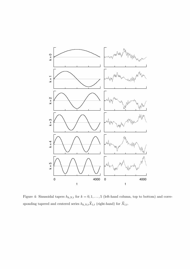
A convenient set of multitapers to use is the family of sinusoidal tapers. These

tapers are easily computed since they are given by

hk,N,t =(

2

N + 1

)1/2

sin

((k + 1)π(t + 1)

N + 1

), t = 0, . . . , N − 1. (22)

The left-hand column of figure 4 shows these tapers for k = 0, 1, . . . , 5. The

right-hand column shows the product of hk,N,t and the clock noise series X1,t. The

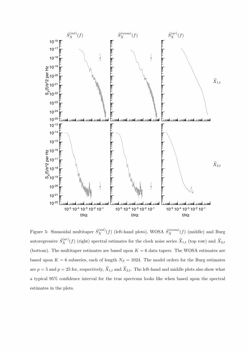
left-hand column of figure 5 shows the K = 6 sinusoidal multitaper estimates for

X1,t (upper plot) and X2,t (lower).

Statistical theory suggests that a 95% confidence interval for the unknown

SX(f) is given by ⎡⎣ νS(mt)X (f)

Qν(0.975),νS

(mt)X (f)

Qν(0.025)

⎤⎦ , (23)

where here ν = 2K, and Qν(p) is the percentage point such that the probability

of a chi-square random variable with ν degrees of freedom being less than Qν(p)

is p (when K = 6 so that ν = 2K = 12, we have Q12(0.025).= 4.404 and

Q12(0.975).= 23.337). The width of such a confidence interval on a log/log plot

is independent of the actual value of S(mt)X (f). The confidence interval based

upon a fictitious estimate S(mt)X (0.1) = 10−18 is shown in the upper left-hand plot

of figure 5 and can be used to roughly gauge the variability we can expect the

multitaper estimator to have. In addition, for 0 < f ′j < f ′

j′ < fN , we can expect

the estimators S(mt)X (f ′

j) and S(mt)X (f ′

j′) to be approximately uncorrelated as long

as the separation between frequencies f ′j′ −f ′

j is at least as large as the bandwidth

of the multitaper estimator, which is given by K+1(N+1)∆t

.



The choice of K dictates the statistical properties of S(mt)X (f). As K increases,

Equation (21) says that more averaging is used to form the estimator, which results

in a decrease in the variance of S(mt)X (f) and in a tighter confidence interval for

the unknown SX(f). Since the variance of S(mt)X (f) is proportional to 1/K, there

is a rapid drop in variability as we initially increase K beyond unity. Setting K

to be in the range of 5 to 10 yields an estimator with a reduction in variance that

is a clear improvement over the variability inherent in the periodogram (compare

the left-hand plots in figures 2 and 5). As K increases, the bandwidth of the

estimator also increases, which unfortunately can offset some of the advantages

of decreased variability. In particular, if the true spectrum has a sharp peak,

increasing the bandwidth will broaden the peak in the estimated spectrum, thus

increasing uncertainty in its location. If the bandwidth is too large, two peaks

that are separated by less than the bandwidth can be smeared together by the

estimator. Restricting K to be in the range of 5 to 10 has the additional benefit

of keeping the bandwidth small enough so that the estimated spectrum reliably

preserves sharp features in most applications.

3.3. Welch’s Overlapped Segment Averaging Spectral Estimation

While multitapering is one strategy for obtaining a spectral estimator with better

properties than the periodogram, another commonly used approach is Welch’s

overlapped segment averaging (WOSA) spectral estimator [47]. The idea is to

break the centered time series Xt up into overlapping subseries of equal length, to

apply a common data taper to each subseries and then to form an estimator based

upon averaging the squared magnitudes of the DFTs of each tapered subseries.

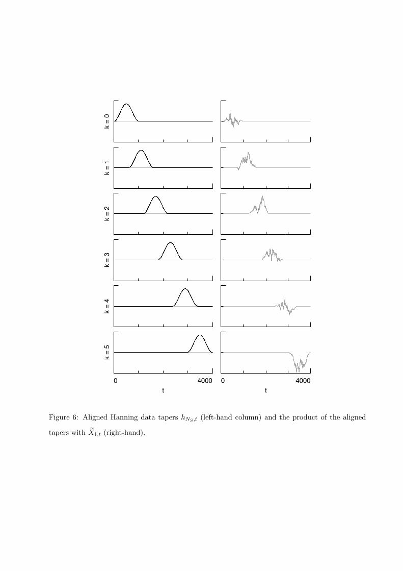
Let NS represent the length of each subseries, and let K be the number of

subseries, with the individual subseries being indexed by k = 0, 1, . . . , K − 1.

Figure 6 illustrates the tapering of K = 6 subseries from X1,t, each of length


Donald B Percival

NS = 1024. Here we take the common taper to be the Hanning data taper hNS ,t

of equation (18). The kth subseries consists of X1,tk , X1,tk+1, . . . , X1,tk+NS−1, where

the starting indices are given by

tk =⌊k

(N − NS

K − 1

)⌋, k = 0, 1, . . . , K − 1 (24)

(in the above, �x� is the greatest integer that is less than or equal to x). The

left-hand column of plots shows the Hanning data taper aligned to t0 = 0, t1 = 595,

. . . , t5 = 2976. The right-hand column shows the product of each aligned hNS ,t

with X1,t. Note that, except at the extremes of the time series, values that happen

to be severely tapered in one subseries are relatively unaltered in an adjacent

subseries. For the Hanning data taper, it is recommended that, once NS has been

selected, the number of subseries K be set so that the overlap between adjacent

subseries is about 50%. For the example, the overlap is 1 − N−NS

NS(K−1)= 41.9%.

Since we can select the subseries length NS to be a power of two, it is easy

to formulate the WOSA estimator to take advantage of an FFT algorithm that

requires a power of two. For a bit more generality, we formulate the estimator

in terms of N ′, which we take to be any power of two satisfying N ′ ≥ NS. With

h′NS ,t defined in terms of hNS ,t as per equation (19), the WOSA spectral estimator

is given by

S(wosa)X (f ′

j) =∆t

K

K−1∑k=0

∣∣∣∣∣∣N ′−1∑t=0

h′NS ,tX

′t+tk

e−i2πtj/N ′

∣∣∣∣∣∣2

, j = 0, 1, . . . ,N ′

2. (25)

If N ′ is set to the same power of two in the above and in equation (21), the WOSA

and multitaper estimates are computed over the same grid of frequencies.

The middle column of figure 5 shows the WOSA spectral estimates for the

clock noise series X1,t (top plot) and X2,t (bottom). To get an idea of how

much sampling variability there is in the WOSA estimator, the upper plot also

shows a 95% confidence interval for the true spectrum at f = 0.1 based upon a

fictitious estimate of S(wosa)X (0.1) = 10−18. This interval is computed as indicated



by equation (23), but we need to replace S(mt)X (f) with S

(wosa)X (f) and to set ν

using

ν =2K

1 + 2∑K−1

k=1

(1 − k

K

) ∣∣∣∑NS−1t=0 hNS ,thNS ,t+tk

∣∣∣2 . (26)

For the present example, this yields ν.= 11.9, which is virtually the same as for the

multitaper estimates (ν = 12). If the degree of overlap between adjacent subseries

is close to 50% (as is the case in our example), then, to a good approximation,

the above becomes

ν ≈ 2K

1 + 2(K−1)K

∣∣∣∑NS/2−1t=0 hNS ,thNS ,t+NS/2

∣∣∣2 ≈ 36K2

19K − 1. (27)

The second approximation above yields ν.= 11.5. Finally, we note that the

bandwidth for the Hanning-based WOSA estimator is approximately 2NS ∆t

, which

implies that S(wosa)X (f ′

j) and S(wosa)X (f ′

j′) with 0 < f ′j < f ′

j′ < fN are uncorrelated

to a reasonable approximation as along as f ′j′ − f ′

j is at least as large as this

bandwidth.

3.4. Autoregressive Spectral Estimation

The spectral estimators that we have discussed in the previous three subsections

are formed based upon one or more DFTs of either part or all of a time series

(after centering and possibly tapering). An alternative approach that is quite

effective for typical clock noise is to use an autoregressive (AR) process to model

Xt. Under this model, we presume that

Xt = µ +p∑

k=1

φp,k(Xt−k − µ) + εt, (28)

where µ is a constant representing the expected value of Xt; p is the order of the

AR model; φp,1, φp,2, . . . , φp,p are constants known as the AR coefficients; and εt

is a set of uncorrelated random variables with mean zero and variance σ2p (i.e., εt


Donald B Percival

is white noise). An AR process has an associated theoretical spectrum given by

SX(f) =σ2

p ∆t

|1 − ∑pk=1 φp,ke−i2πfk ∆t|2

, |f | ≤ fN . (29)

The scheme is to plug estimates φp,1, φp,2, . . . , φp,p and σ2p of the p+1 AR parameters

into the above to create an AR spectral estimator S(ar)X (f). Note that we can use

the DFT to evaluate this estimator over the same grid of frequencies f ′k as before.

To do so, define

φ′p,k =

⎧⎪⎪⎪⎪⎪⎪⎨⎪⎪⎪⎪⎪⎪⎩1, k = 0;

−φp,k, k = 1, . . . , p; and

0, k = p + 1, p + 2, . . . .

(30)

Then

S(ar)X (f ′

j) =σ2

p ∆t∣∣∣∑N ′−1k=0 φ′

p,ke−i2πkj/N ′

∣∣∣2 , j = 0, . . . , N ′/2. (31)

There are many estimators in the literature for the AR parameters. For typical

clock noise spectra, we recommend the Burg estimator [11], which is remarkably

effective and can be computed efficiently [10, 25, 27, 35, 42]. For t = 0, . . . , N −1,

define f0,t = Xt and b0,t = Xt. Let A1 = 2Nσ2X − X2

0 − X2N−1 and σ2

0 = σ2X , where

σ2X is the sample variance of Xt. We obtain the estimators φp,1, φp,2, . . . , φp,p and

σ2p by recursively computing, for l = 1, . . . , p,

Bl = 2N−1∑t=l

fl−1,tbl−1,t−l (32)

φl,l = Bl/Al (33)

φl,k = φl−1,k − φl,lφl−1,l−k, 1 ≤ k ≤ l − 1 (this is skipped if l = 1) (34)

σ2l = σ2

l−1(1 − φ2l,l) (35)

fl,t = fl−1,t − φl,lbl−1,t−l, l ≤ t ≤ N − 1 (36)

bl,t−l = bl−1,t−l − φl,lfl−1,t, l ≤ t ≤ N − 1 (37)

Al+1 =(1 − φ2

l,l

)Al − f 2

l,l − b2l,N−l−1 (38)

(the last three equations can be skipped when l = p). The desired estimators of

the p + 1 AR parameters are available as output at the end of the pth recursion.



Equation (34) is also part of the Levinson–Durbin recursions that are used to form

the well-known Yule–Walker estimator of the AR parameters [25, 27, 35, 42].

The remaining task is to set p. Three approaches are to use Akaike’s final

prediction error (FPE) [1], Akaike’s information criterion (AIC) [2] or the Bayesian

information criterion (BIC) [40]. All three criteria require that we initially set p

to some maximum value, say p′, and use the Burg method to fit a model of order

p′ to the data, keeping track of σ2l , l = 1, . . . , p′, as they are computed as part of

the Burg recursive equations. The FPE approach consists of plotting

FPE(l) =N + l + 1

N − l − 1σ2

l (39)

versus l = 1, . . . , p′ and then setting p to the value of l for which FPE(l) is the

smallest. The AIC approach is similar in spirit, with FPE(l) being replaced by

AIC(l) = log (σ2l ) +

2l

N(40)

(a ‘bias corrected’ version of the AIC has also been proposed [43, 22], which

consists of replacing 2l/N with 2(l + 1)/(N − l − 2)). The BIC approach makes

use of

BIC(l) = log (σ2l ) +

2 log (N)

N(41)

(for the AIC and BIC, ‘log’ should interpreted as ‘log base e’). In practice, caution

must be exercised in using these criteria since they do not always yield satisfactory

choices for p, but they are often good starting points.

The right-hand column of figure 5 shows the Burg AR spectral estimates for

the two clock noise series. With p′ set to 100, we used the FPE criterion to set

p = 5 and 25 for, respectively, X1,t and X2,t. While the two estimated AR spectra

are much smoother looking than either the multitaper or WOSA estimates, it is

not easy to assess the effect of sampling variability, and hence we cannot display

a 95% confidence interval here as we could in the left-hand and middle columns.

It is also not easy to give a measure of the bandwidth of S(ar)X (f). Despite these


Donald B Percival

limitations, the Burg AR spectral estimator is guaranteed to integrate to the

sample variance as per equation (2).

3.5. Prewhitening and Postcoloring

A technique that can potentially improve the spectral estimators we have discussed

so far is prewhitening. The basic idea is to filter a time series so that the output

from the filter is closer to white noise than the unfiltered series. We then perform

a spectral analysis on the filtered series and estimate the spectrum for the original

(unfiltered) series using the estimate based on the filtered series after it has been

adjusted for the effect of the prewhitening filter. The rationale for this scheme is

that the spectrum for white noise is much easier to estimate for any other process

since it is just a constant proportional to the variance of the process. When

presented with white noise, all of the estimators we have considered so far are

unbiased estimators of the true spectrum. In practice, prewhitening often works

well even if the spectrum for the filtered series is still markedly different from

white noise.

For processes whose spectra are dominated by low frequency components,

a commonly used prewhitening filter is a first-order backward difference. Such

a filter damps down low frequency components considerably and is useful for

intrinsically stationary processes as long as the spectrum for the differenced process

does not damp down to zero too fast as f → 0. In the context of clock noise, the

first-order backward difference X(1)t = Xt −Xt−1 is proportional to the fractional

frequency deviation Y t = (Xt − Xt−1)/∆t, so we will consider the latter instead

of X(1)t . The spectra for Y t and Xt are related by

SY (f) =4 sin2(πf ∆t)

(∆t)2SX(f). (42)



Once we have estimated SY (f) using, say, SY (f), we can estimate SX(f) using

SX(f) =(∆t)2

4 sin2(πf ∆t)SY (f). (43)

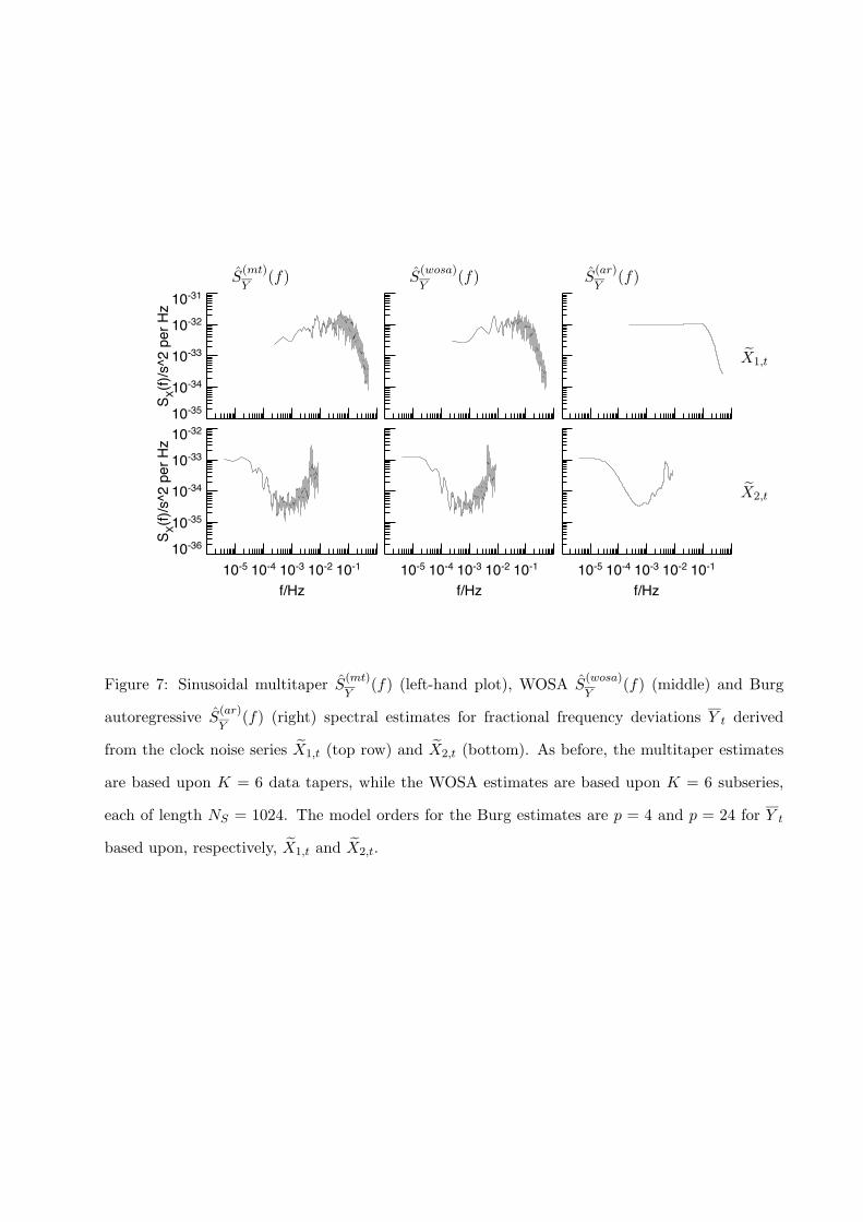
Figure 7 shows multitaper, WOSA and AR spectral estimates based upon

Y t for the two clock noise series X1,t and X2,t (the plots are arranged in the

same manner as for figure 5). These estimates were obtained by using Y t (after

centering and possible zero padding) in place of Xt or X ′t in all the equations

stated previously in this section. For the AR estimates, the FPE criterion picked

out p = 4 and 24 for the two fractional frequency series, in contrast to 5 and

25 for X1,t and X2,t. Whereas the spectra in figure 5 have variations ranging

over 7 or 8 decades, the ones in figure 7 range only over about 2 decades, so the

first-order backward difference filter has indeed had a whitening effect. There

is, however, some concern with the AR estimate corresponding to X1,t (upper

right-hand plot). The corresponding multitaper and WOSA estimates show the

spectra to be decreasing as f → 0, whereas the AR estimate flattens out. This

points out a potential problem with AR spectral estimates, namely that, whereas

they have been demonstrated to work well with processes whose spectra increase

as f → 0, they are also known to perform poorly in comparison to multitaper and

WOSA estimators for processes whose spectra decrease rapidly as f → 0. (In fact,

prewhitening is rarely used with AR spectral estimation, but, rather, low-order

AR models are often fit to a time series to identify a potential prewhitening filter;

for more details, see, e.g., [35], section 9.10).

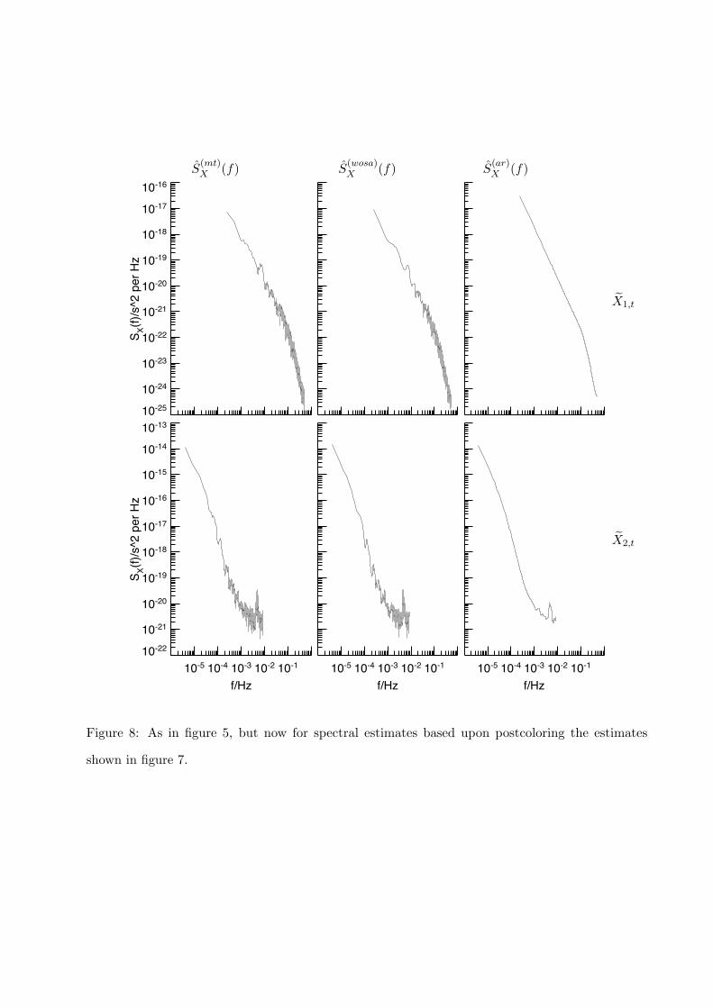
Figure 8 shows the multitaper, WOSA and AR spectral estimates for SX(f)

based upon converting the estimates for SY (f) in figure 7 using equation (43).

The agreement amongst the three spectra is quite good, with the exception

that the AR estimate for X1,t (upper right-hand plot) is elevated about half an

order of magnitude above the multitaper and WOSA estimates at the very lowest

frequency. This discrepancy can be attributed to the deficiency in AR spectral


Donald B Percival

estimation that we just pointed out. If we compare the multitaper and WOSA

spectra in figures 8 with those in figure 5, again the agreement is quite good except

at the very lowest frequencies. The ones in figure 5 tend to flatten out, whereas

those in figure 8 do not. The tendency of the estimates in figure 5 to flatten out

can be attributed to the bandwidth of these estimates, which begin to trap the

value f = 0 at the very lowest frequencies. Because of the need to center the

time series, the estimated spectra are biased toward zero at frequencies that are

less than a bandwidth away from f = 0. The prewhitening scheme has evidently

removed some of this bias, so the multitaper and WOSA spectra in figures 8 are

to be preferred over those in figure 5.

3.6. Comparison of Spectral Estimators

Let us now take a closer look at the multitaper and WOSA spectral estimates of

figure 8 and the AR spectral estimates of figure 5. Note that the AR spectral

estimates are much smoother than the multitaper and WOSA estimates. In

principle, the multitaper estimate could be smoothed out by increasing K, and the

WOSA also, by increasing K along with a reduction in NS (we could also decrease

the variability in the estimates by smoothing across frequencies); however, there is

no compelling reason for smoothing here since the variability in the multitaper and

WOSA estimates is not so large that we cannot easily see how the spectra vary with

frequency. The advantage of the relatively unsmoothed multitaper and WOSA

estimates over the AR estimates is that their statistical properties are tractable,

and hence they are suitable for future manipulations (see the discussion in the

next section). While the AR spectral estimates are certainly quite good, their

statistical properties are difficult to assess without some rather strong assumptions

(in particular, that there is no error in the selected order p).

Visually the multitaper, WOSA and AR spectral estimates follow the same



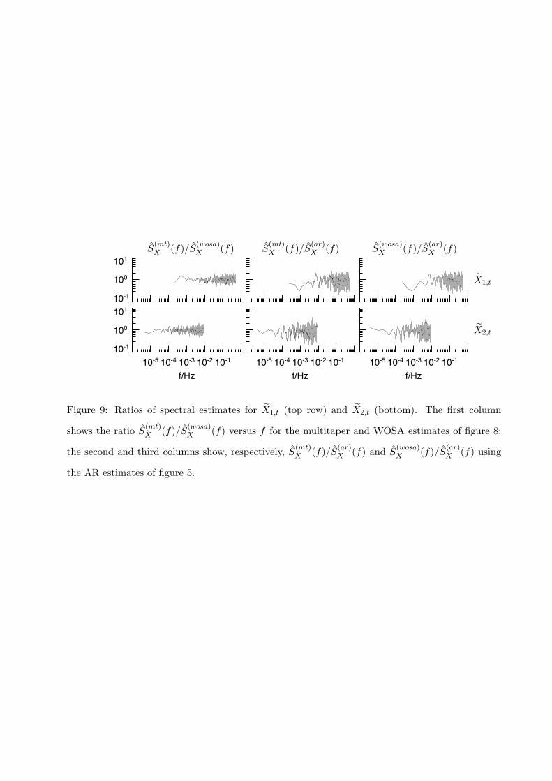
overall patterns as functions of frequency. For a more sensitive comparison, the

top row of plots in figure 9 shows, from left to right, the ratios S(mt)X (f)/S

(wosa)X (f),

S(mt)X (f)/S

(ar)X (f) and S

(wosa)X (f)/S

(ar)X (f) for X1,t, while the bottom row is for X2,t.

Despite the inherently bumpy nature of the multitaper and WOSA estimates, the

left-hand column of plots show that, except at a very few isolated frequencies,

they differ by no more than a factor of two. The general conclusion that we can

draw from figure 9 is that, although the three estimators we have discussed have

quite different theoretical foundations, they are all telling us the same story about

the spectra of X1,t and X2,t.

4. Uses for the Spectrum in Assessing Clock Noise

In this section we briefly mention some of the uses for the spectrum SX(f) and

its estimates SX(f) in assessing the performance of clocks. Since Xt involves a

comparison between two clocks, the estimated spectrum reflects the performance

of both. If one of the clocks in the comparison is regarded as an approximation to

a ‘noise free’ standard, then the spectrum will largely reflect the performance of a

clock under test. A direct comparison of the levels of the estimated spectra for two

clocks under test can reveal ranges of Fourier frequencies over which one clock is

superior. While such comparisons are the most obvious use for estimated spectra,

in fact spectra can contribute to the characterization of clock noise in several

other ways. (In passing, we note that, when intercomparing three or more clocks,

none of which can be regarded as a ‘noise free’ standard, it is in theory possible

to obtain an estimate of the spectrum for an individual clock by examining the

cross-spectrum between contemporaneous measurements of X1,t and X2,t, both of

which involve the individual clock of interest. To make this work, there is a critical

assumption, namely, that all three clocks involved in the two sets of measurements

are uncorrelated with one another.)


Donald B Percival

First, estimated spectra can be used to provide a nonparametric method

for assessing the variability in time-domain measures of clock instability. A

well-known such measure is the Allan variance [3, 5]. For moderate sample sizes

N , the distribution of the maximal-overlap estimator of the Allan variance is, to

a good approximation, normally distributed with a mean given by the population

Allan variance and with a variance that is proportional to

∫ fN

−fNAτ (f)S2

X(f) df, (44)

where Aτ (f) can be computed based upon knowledge of the filter whose squared

output forms the basis for the maximal-overlap estimator at averaging time τ [33,

36]. A nonparametric method for assessing the variability in the estimated Allan

variance is to use SX(f) in place of SX(f) in the above. The current procedure

for assessing variability is parametric and involves associating Xt with a canonical

power-law process [17]. This nonparametric approach is simpler, is asymptotically

correct, and avoids the canonical power-law assumptions behind the parametric

approach. (The above remarks hold for time-domain characterizations of clock

noise other than the Allan variance.)

Second, the estimated spectra can be used to assess the power-law assumption

underlying the statistical assessment of most time-domain characterizations of

clock noise. A glance at the estimated spectra for the two examples we have

examined shows that, while the spectrum for X1,t might be well-modeled as

a piece-wise power-law process, the spectrum for X2,t is not, particularly, for

frequencies between fN/2 and fN .

Third, estimates of the spectrum can be used to assess the validity of the

hypothesis that one of the canonical power-law spectra (i.e., SX(f) = |f |α, with

α = 0, −1, −2, −3 or −4) is tenable as a spectral model over a certain range of

frequencies for a given set of clock noise measurements. Here the fact that the

multitaper and WOSA estimators have tractable statistical properties plays an



important role because it is possible to compute an estimate α of α based upon a

linear least squares fit of log (SX(f)) versus log(f) and to assess the variability in

α [28, 29, 34]. Using statistical methodology to assess the validity of the canonical

power-law hypothesis has generally been ignored in practice, but it is important

to test as much as possible the assumptions underlying any statistical analysis to

avoid incorrect inferences.

Fourth, the development of new statistical measures for characterizing clock

noise in the time domain continues to be an area of active research, which is

evidence that no existing time domain measure is fully satisfactory (see, e.g.,

[20]). To date, all such measures are similar to the Allan variance in the sense of

being based on the squared outputs from non-ideal band-pass filters. Comparison

between old and new measures would be easier if there were a ‘gold standard.’

In the frequency domain, there is an obvious choice, namely, an ideal band-pass

variance, which by definition would be just the integral of the spectrum SX(f)

over the relevant pass-band [39, 32]. New and existing time domain measures can

be evaluated as estimators of this target variance in terms of, e.g., bias, variance

and mean squared error. This approach would lead to a viable way of objectively

determining whether or not one measure is superior to another when analyzing a

certain type of clock noise.

5. Summary

We have demonstrated that three different spectral estimators (multitaper, WOSA

and autoregressive) yield basically the same results when applied to two representative

clock noise series. Clock noise spectra can thus be successfully tackled using any

of these estimators, even though the estimation of power spectra is in general

complicated due to the wide variety of spectra that are encountered in the engineering

and physical sciences. The theoretical underpinnings of these three estimators are


Donald B Percival

quite different. The fact that the end results are in such good agreement reassures

us that our estimates are on target. Given a routine that efficiently computes

the discrete Fourier transform, we have given all the equations needed to fully

implement all three estimators. Finally, we have noted some important uses for

spectra and their estimates in the statistical characterization of clock noise, both

in the frequency and time domains.

In passing we note that the spectral analyses we have presented demonstrate

the effectiveness of autoregressive processes as models for clock noise. The problem

of forming a time scale based upon an ensemble of clocks can be formulated as a

Kalman filter (see, e.g., [16] and references therein), but this approach has been

problematic in that such a filter cannot easily handle the canonical power-law

processes with α = −1 and α = −3 (phase and frequency flicker noises). The

Kalman filter, however, can readily accommodate autoregressive processes [24],

so a promising avenue of research would be to use just autoregressive processes

(with appropriate parameter estimation) as clock noise models.

6. Software and Acknowledgments

A collection of functions in the freeware statistical package R that implements

the procedures described here is available upon request from the author. The R

package itself can be downloaded from the Comprehensive R Archive Network at

http://cran.r-project.org/.

The author would like to thank (i) the National Institute of Standards and

Technology, Time and Frequency Division, for support and (ii) Demetrios Matsakis,

Lara Schmidt and Sam Stein for the clock noise data.



References

1. Akaike H 1970 Statistical predictor identification Annals of the Institute of

Statistical Mathematics 22 203–17

2. Akaike H 1974 A new look at the statistical model identification IEEE

Transactions on Automatic Control 19 716–22

3. Allan D W 1966 Statistics of atomic frequency standards Proceedings of the

IEEE 54 221–30

4. Anderson T W 1971 The Statistical Analysis of Time Series (New York: John

Wiley & Sons) 704 p.

5. Barnes J A, Chi A R, Cutler L S, Healey D J, Leeson D B, McGunigal T

E, Mullen Jr J A, Smith W L, Sydnor R L, Vessot R F C, and Winkler

G M R 1971 Characterization of frequency stability IEEE Transactions on

Instrumentation and Measurement 20 105–20.

6. Blackman R B and Tukey J W 1958 The Measurement of Power Spectra (New

York: Dover Publications) 190 p.

7. Bloomfield P 2000 Fourier Analysis of Time Series: An Introduction 2nd edn

(New York: John Wiley & Sons) 261 p.

8. Brillinger D R 1981 Time Series: Data Analysis and Theory expanded edn

(San Francisco: Holden–Day) 540 p.

9. Brockwell P J and Davis R A 1991 Time Series: Theory and Methods 2nd

edn (New York: Springer–Verlag) 577 p.

10. Brockwell P J and Davis R A 2002 Introduction to Time Series and Forecasting

2nd edn (New York: Springer) 434 p.

11. Burg J P 1968 A new analysis technique for time series data NATO Advanced

Study Institute on Signal Processing with Emphasis on Underwater Acoustics;

also in Childers D G 1978 Modern Spectrum Analysis (New York: IEEE Press)

334 p.


Donald B Percival

12. Chan G, Hall P and Poskitt D S 1995 Periodogram-based estimators of fractal

properties Annals of Statistics 23 1684–711

13. Chatfield C 2004 The Analysis of Time Series: An Introduction 6th edn (Boca

Raton, LA: Chapman & Hall/CRC) 333 p.

14. Fougere P F 1985 On the accuracy of spectrum analysis of red noise processes

using maximum entropy and periodogram methods: simulation studies and

application to geophysical data Journal of Geophysical Research 90 4355–66

15. Fuller W A 1996 Introduction to Statistical Time Series 2nd edn (New York:

John Wiley & Sons) 698 p.

16. Galleani L and Tavella P 2003 On the use of the Kalman filter in timescales

Metrologia 40 S326–34

17. Greenhall C A 1991 Recipes for degrees of freedom of frequency stability

estimators IEEE Transactions on Instrumentation and Measurement 40

994–9.

18. Grenander U and Rosenblatt M 1984 Statistical Analysis of Stationary Time

Series 2nd edn (New York: Chelsea Publishing Company) 308 p.

19. Hamilton J D 1994 Time Series Analysis (Princeton, NJ: Princeton University

Press) 799 p.

20. Howe D A 2006 TheoH: a hybrid, high-confidence statistic that improves on

the Allan deviation Metrologia under revision

21. Hurvich C M and Ray B K 1995 Estimation of the memory parameter for

nonstationary or noninvertible fractionally integrated processes Journal of

Time Series Analysis 16 17–41

22. Hurvich C M and Tsai C–L 1989 Regression and time series model selection

in small samples Biometrika 76 297–301

23. Jenkins G M and Watts D G 1968 Spectral Analysis and Its Applications (San

Francisco, CA: Holden–Day) 525 p.



24. Jones R H 1980 Maximum likelihood fitting of ARMA Models to time series

with missing observations Technometrics 22 389–95

25. Kay S M 1988 Modern Spectral Estimation: Theory and Application

(Englewood Cliffs, NJ: Prentice–Hall) 543 p.

26. Koopmans L H 1995 The Spectral Analysis of Time Series 2nd edn (San

Diego, CA: Academic Press) 366 p.

27. Marple S L Jr 1987 Digital Spectral Analysis with Applications (Englewood

Cliffs, NJ: Prentice–Hall) 492 p.

28. McCoy E J, Walden A T and Percival D B 1998 Multitaper spectral estimation

of power law processes IEEE Transactions on Signal Processing 46 655–68.

29. Nichols–Pagel G A, Percival D B and Reinhall P G 2006 Should structure

functions be used to estimate power laws in turbulence? A comparative study

Physica D under revision

30. Oppenheim A V and Schafer R W 1989 Discrete-Time Signal Processing

(Englewood Cliffs, NJ: Prentice–Hall) 879 p.

31. Papoulis A and Pillai S U 2002 Probability, Random Variables, and Stochastic

Processes 4th edn (New York: McGraw–Hill) 304 p.

32. Percival D B 1991 Characterization of frequency stability: frequency domain

estimation of stability measures Proceedings of the IEEE 79 961–72

33. Percival D B 1995 On estimation of the wavelet variance Biometrika 82 619–31

34. Percival D B 2003 Stochastic models and statistical analysis for clock noise

Metrologia 40 S289–304

35. Percival D B and Walden A T 1993 Spectral Analysis for Physical Applications:

Multitaper and Conventional Univariate Techniques (Cambridge, UK:

Cambridge University Press) 583 p.

36. Percival D B and Walden A T 2000 Wavelet Methods for Time Series Analysis

(Cambridge, UK: Cambridge University Press) 594 p.


Donald B Percival

37. Priestley M B 1981 Spectral Analysis and Time Series (London: Academic

Press) 890 p.

38. Riedel K S and Sidorenko A 1995 Minimum bias multiple taper spectral

estimation IEEE Transactions on Signal Processing 43 188–95

39. Rutman J 1978 Characterization of phase and frequency instabilities in

precision frequency sources: fifteen years of progress Proceedings of the IEEE

66 1048–75

40. Schwarz G 1978 Estimating the dimension of a model Annals of Statistics 6

461–4

41. Shumway R H and Stoffer D S 2006 Time Series Analysis and Its Application

2nd edn (New York: Springer) 592 p.

42. Stoica P and Moses R L 1997 Introduction to Spectral Analysis (Upper Saddle

River, NJ: Prentice Hall) 319 p.

43. Sugiura N 1978 Further analysis of the data by Akaike’s information criterion

and the finite corrections Communications in Statistics: Theory and Methods

7 13–26

44. Thomson D J 1982 Spectrum estimation and harmonic analysis Proceedings

of the IEEE 70 1055–96

45. Velasco C 1999 Gaussian semiparametric estimation of non-stationary time

series Journal of Time Series Analysis 20 87–127

46. Velasco C 1999 Non-stationary log-periodogram regression Journal of

Econometrics 91 325–71

47. Welch P D 1967 The use of fast Fourier transform for the estimation of power

spectra: a method based on time averaging over short, modified periodograms

IEEE Transactions on Audio and Electroacoustics 15 70–3

48. Yaglom A M 1958 Correlation theory of processes with random stationary nth

increments American Mathematical Society Translations (Series 2) 8 87–141



49. Yaglom A M 1987 Correlation Theory of Stationary and Related Random

Functions, Volume I: Basic Results (New York: Springer–Verlag) 526 p.

Received on xx xxxx 2006.


Donald B Percival

Figure captions

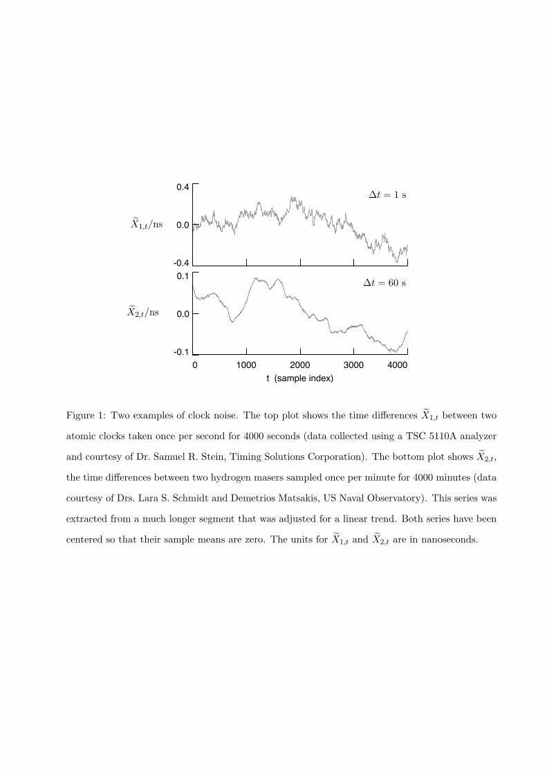
1. Two examples of clock noise. The top plot shows the time differences X1,t

between two atomic clocks taken once per second for 4000 seconds (data

collected using a TSC 5110A analyzer and courtesy of Dr. Samuel R. Stein,

Timing Solutions Corporation). The bottom plot shows X2,t, the time

differences between two hydrogen masers sampled once per minute for 4000

minutes (data courtesy of Drs. Lara S. Schmidt and Demetrios Matsakis, US

Naval Observatory). This series was extracted from a much longer segment

that was adjusted for a linear trend. Both series have been centered so that

their sample means are zero. The units for X1,t and X2,t are in nanoseconds.

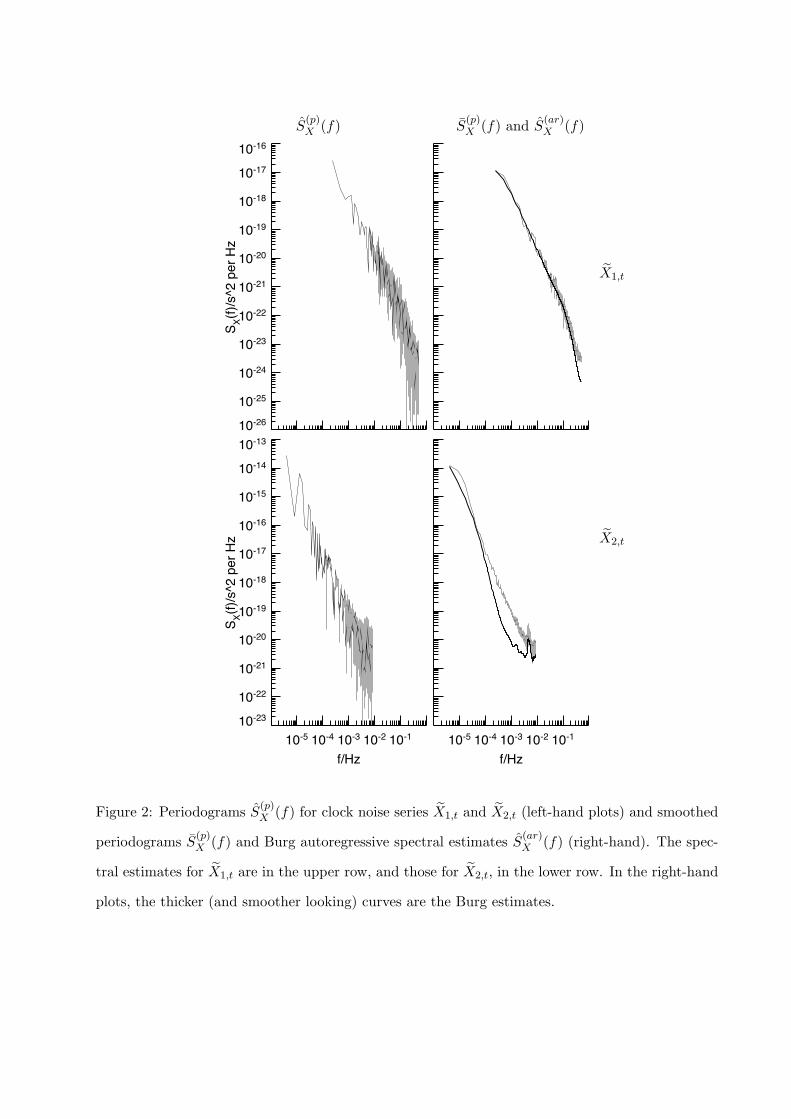
2. Periodograms S(p)X (f) for clock noise series X1,t and X2,t (left-hand plots) and

smoothed periodograms S(p)X (f) and Burg autoregressive spectral estimates

S(ar)X (f) (right-hand). The spectral estimates for X1,t are in the upper row,

and those for X2,t, in the lower row. In the right-hand plots, the thicker

(and smoother looking) curves are the Burg estimates.

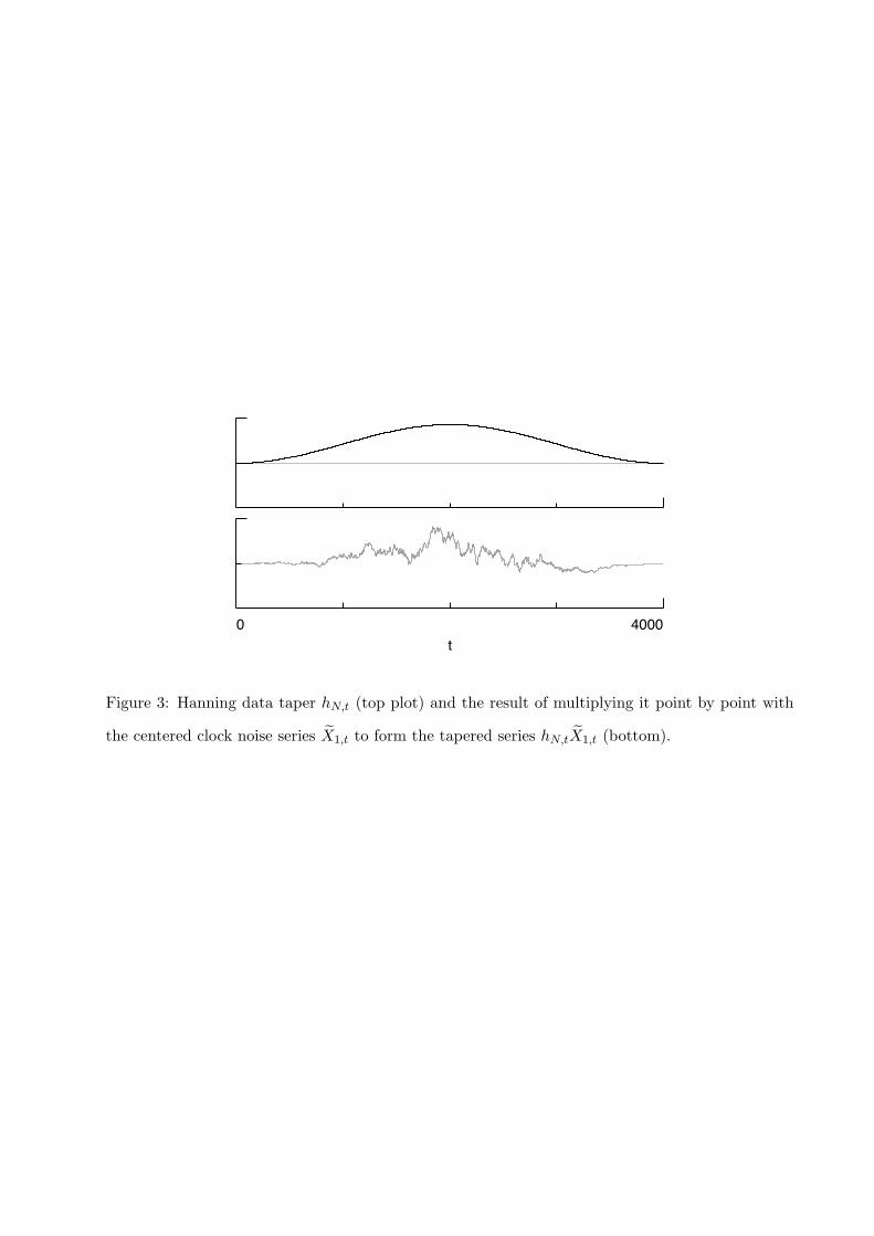
3. Hanning data taper hN,t (top plot) and the result of multiplying it point

by point with the centered clock noise series X1,t to form the tapered series

hN,tX1,t (bottom).

4. Sinusoidal tapers hk,N,t for k = 0, 1, . . . , 5 (left-hand column, top to bottom)

and corresponding tapered and centered series hk,N,tX1,t (right-hand) for

X1,t.

5. Sinusoidal multitaper S(mt)X (f) (left-hand plots), WOSA S

(wosa)X (f) (middle)

and Burg autoregressive S(ar)X (f) (right) spectral estimates for the clock

noise series X1,t (top row) and X2,t (bottom). The multitaper estimates

are based upon K = 6 data tapers. The WOSA estimates are based upon



K = 6 subseries, each of length NS = 1024. The model orders for the

Burg estimates are p = 5 and p = 25 for, respectively, X1,t and X2,t. The

left-hand and middle plots also show what a typical 95% confidence interval

for the true spectrum looks like when based upon the spectral estimates in

the plots.

6. Aligned Hanning data tapers hNS ,t (left-hand column) and the product of

the aligned tapers with X1,t (right-hand).

7. Sinusoidal multitaper S(mt)

Y(f) (left-hand plot), WOSA S

(wosa)

Y(f) (middle)

and Burg autoregressive S(ar)

Y(f) (right) spectral estimates for fractional

frequency deviations Y t derived from the clock noise series X1,t (top row) and

X2,t (bottom). As before, the multitaper estimates are based upon K = 6

data tapers, while the WOSA estimates are based upon K = 6 subseries,

each of length NS = 1024. The model orders for the Burg estimates are

p = 4 and p = 24 for Y t based upon, respectively, X1,t and X2,t.

8. As in figure 5, but now for spectral estimates based upon postcoloring the

estimates shown in figure 7.

9. Ratios of spectral estimates for X1,t (top row) and X2,t (bottom). The

first column shows the ratio S(mt)X (f)/S

(wosa)X (f) versus f for the multitaper

and WOSA estimates of figure 8; the second and third columns show,

respectively, S(mt)X (f)/S

(ar)X (f) and S

(wosa)X (f)/S

(ar)X (f) using the AR estimates

of figure 5.


-0.4

0.0

0.4

-0.1

0.0

0.1

0 1000 2000 3000 4000

t (sample index)

∆t = 1 s

∆t = 60 s

X1,t/ns

X2,t/ns

Figure 1: Two examples of clock noise. The top plot shows the time differences X1,t between two

atomic clocks taken once per second for 4000 seconds (data collected using a TSC 5110A analyzer

and courtesy of Dr. Samuel R. Stein, Timing Solutions Corporation). The bottom plot shows X2,t,

the time differences between two hydrogen masers sampled once per minute for 4000 minutes (data

courtesy of Drs. Lara S. Schmidt and Demetrios Matsakis, US Naval Observatory). This series was

extracted from a much longer segment that was adjusted for a linear trend. Both series have been

centered so that their sample means are zero. The units for X1,t and X2,t are in nanoseconds.

10-26

10-25

10-24

10-23

10-22

10-21

10-20

10-19

10-18

10-17

10-16

SX(f

)/s^

2 pe

r H

z

10-5 10-4 10-3 10-2 10-1

f/Hz

10-23

10-22

10-21

10-20

10-19

10-18

10-17

10-16

10-15

10-14

10-13

SX(f

)/s^

2 pe

r H

z

10-5 10-4 10-3 10-2 10-1

f/Hz

S(p)X (f) S

(p)X (f) and S

(ar)X (f)

X1,t

X2,t

Figure 2: Periodograms S(p)X (f) for clock noise series X1,t and X2,t (left-hand plots) and smoothed

periodograms S(p)X (f) and Burg autoregressive spectral estimates S

(ar)X (f) (right-hand). The spec-

tral estimates for X1,t are in the upper row, and those for X2,t, in the lower row. In the right-hand

plots, the thicker (and smoother looking) curves are the Burg estimates.

0 4000t

Figure 3: Hanning data taper hN,t (top plot) and the result of multiplying it point by point with

the centered clock noise series X1,t to form the tapered series hN,tX1,t (bottom).

k =

0k

= 1

k =

2k

= 3

k =

4k

= 5

0 4000

t

0 4000

t

Figure 4: Sinusoidal tapers hk,N,t for k = 0, 1, . . . , 5 (left-hand column, top to bottom) and corre-

sponding tapered and centered series hk,N,tX1,t (right-hand) for X1,t.

10-25

10-24

10-23

10-22

10-21

10-20

10-19

10-18

10-17

10-16

SX(f

)/s^

2 pe

r H

z

x x

10-22

10-21

10-20

10-19

10-18

10-17

10-16

10-15

10-14

10-13

SX(f

)/s^

2 pe

r H

z

10-5 10-4 10-3 10-2 10-1

f/Hz

x

10-5 10-4 10-3 10-2 10-1

f/Hz

x

10-5 10-4 10-3 10-2 10-1

f/Hz

S(mt)X (f) S

(wosa)X (f) S

(ar)X (f)

X1,t

X2,t

Figure 5: Sinusoidal multitaper S(mt)X (f) (left-hand plots), WOSA S

(wosa)X (f) (middle) and Burg

autoregressive S(ar)X (f) (right) spectral estimates for the clock noise series X1,t (top row) and X2,t

(bottom). The multitaper estimates are based upon K = 6 data tapers. The WOSA estimates are

based upon K = 6 subseries, each of length NS = 1024. The model orders for the Burg estimates

are p = 5 and p = 25 for, respectively, X1,t and X2,t. The left-hand and middle plots also show what

a typical 95% confidence interval for the true spectrum looks like when based upon the spectral

estimates in the plots.

0 4000

t

k =

0k

= 1

k =

2k

= 3

k =

4k

= 5

0 4000

t

Figure 6: Aligned Hanning data tapers hNS ,t (left-hand column) and the product of the aligned

tapers with X1,t (right-hand).

10-35

10-34

10-33

10-32

10-31

SX(f

)/s^

2 pe

r H

z

10-5 10-4 10-3 10-2 10-1

f/Hz

10-36

10-35

10-34

10-33

10-32

SX(f

)/s^

2 pe

r H

z

10-5 10-4 10-3 10-2 10-1

f/Hz10-5 10-4 10-3 10-2 10-1

f/Hz

S(mt)

Y(f) S

(wosa)

Y(f) S

(ar)

Y(f)

X1,t

X2,t

Figure 7: Sinusoidal multitaper S(mt)

Y(f) (left-hand plot), WOSA S

(wosa)

Y(f) (middle) and Burg

autoregressive S(ar)

Y(f) (right) spectral estimates for fractional frequency deviations Y t derived

from the clock noise series X1,t (top row) and X2,t (bottom). As before, the multitaper estimates

are based upon K = 6 data tapers, while the WOSA estimates are based upon K = 6 subseries,

each of length NS = 1024. The model orders for the Burg estimates are p = 4 and p = 24 for Y t

based upon, respectively, X1,t and X2,t.

10-25

10-24

10-23

10-22

10-21

10-20

10-19

10-18

10-17

10-16

SX(f

)/s^

2 pe

r H

z

10-5 10-4 10-3 10-2 10-1

f/Hz

10-22

10-21

10-20

10-19

10-18

10-17

10-16

10-15

10-14

10-13

SX(f

)/s^

2 pe

r H

z

10-5 10-4 10-3 10-2 10-1

f/Hz

10-5 10-4 10-3 10-2 10-1

f/Hz

S(mt)X (f) S

(wosa)X (f) S

(ar)X (f)

X1,t

X2,t

Figure 8: As in figure 5, but now for spectral estimates based upon postcoloring the estimates

shown in figure 7.

10-1

100

101

10-5 10-4 10-3 10-2 10-1

f/Hz

10-1

100

101

10-5 10-4 10-3 10-2 10-1

f/Hz

10-5 10-4 10-3 10-2 10-1

f/Hz

S(mt)X (f)/S

(wosa)X (f) S

(mt)X (f)/S

(ar)X (f) S

(wosa)X (f)/S

(ar)X (f)

X1,t

X2,t

Figure 9: Ratios of spectral estimates for X1,t (top row) and X2,t (bottom). The first column

shows the ratio S(mt)X (f)/S

(wosa)X (f) versus f for the multitaper and WOSA estimates of figure 8;

the second and third columns show, respectively, S(mt)X (f)/S

(ar)X (f) and S

(wosa)X (f)/S

(ar)X (f) using

the AR estimates of figure 5.

spectral analysis of clock noise: a primer

Documents