AGRICULTURAL ECONOMICS

ELSEVIER Agricultural Economics 27 (2002) 403-424 www.elsevier.com/locate/agecon

Spatial economics of biological control: investing in new releases of insects for earlier limitation of Paterson's curse in Australia

T.L. Nordbloma,*, M.J. Smythb, A. Swirepikb, A.W. Sheppardb, D.T. Brieseb,

Cooperative Research Centre for Australian Weed Management (Weeds CRC)

a Farrer Centre, Schaal of Agriculture, Charles Sturt University, Wagga Wagga, NSW 2678, Australia b CSIRO-Entamalagy, GPO Box 1700, Canberra, ACT 2601, Australia

Abstract

Paterson's curse and related weeds (Echiurn spp.) were introduced as garden flowers before 1850 and have spread to over 30 million ha in southern Australia. Four hundred successful releases of crown weevil (M. larvatus) populations specifically targeting Echiurn spp. were made in the 1993-2000 period. Based on the timing, location and performance of these past releases of beneficial insects, spatially and temporally specific trajectories of biocontrol have been simulated. Insect populations established by the past releases are expected to cover expanding areas at densities sufficient to limit host Echiurn infestations only over the next 25-50 years. The present analysis tackles the questions of where and how many additional releases are economically justified to speed up this process. We identify 31 districts in which diminishing niches for further insect releases are projected over time, according to the locations of damaging weed infestations and the timing, location and numbers of past insect releases. Benefits of biocontrol are expressed in terms of the value of recovered pasture productivity, keyed to estimates of loss and to historical district livestock inventories converted to dry sheep equivalent (DSE) feed availability levels to which prices are applied. Expected marginal contributions of increments of new releases were simulated for each of the 31 districts, subject to the space/time limitations of each niche. Our explicit accounting for the spatial and temporal dimensions has made possible the economically optimal targeting of new biocontrol releases. For example, at $12/DSE and a marginal cost of $2000 per release, with a discount rate of 10%, we find there is a case for a program of over 400 new releases targeted to 17 districts, with as few as five releases to each of several and as many as 70 releases in one district. Crown Copyright© 2002 Published by Elsevier Science B.V. All rights reserved.

Keywords: Spatial; Benefit--cost; Investment; Simulation; Classical biological control; Echium spp.; Weed; Magulanes larvatus; Biocontrol agent

1. Introduction

Echiurn plantagineurn (commonly known as Paterson's curse, Salvation Jane or Riverina bluebell)

* Corresponding author. Present address: Economic Services Unit, NSW Agriculture WWAI, Wagga Wagga, NSW 2650, Aus­tralia. Tel.: +61-2-6938-1627; fax: +61-2-6938-1809. E-mail address: tom.nordb1om@agric.nsw.gov.au (T.L. Nordblom).

was introduced to Australia as a garden flower before 1850. An early emerging winter annual plant, it pro­duces abundant seed that may remain viable in the soil for up to 7 years. Free of its native Meditenanean plant and insect communities, it has become one of the dominant pasture weeds of temperate Australia. Other introduced Echiurn species (E. vulgare, E. italicurn and E. simplex) also occur as weeds in Aus­tralia (Parsons and Cuthbertson, 1992). Keeping in

0169-5150/02/$ - see front matter Crown Copyright© 2002 Published by Elsevier Science B.V. All rights reserved. PII: SO 169-5150(02)00069-5

404 T.L. Nordblom et al. I Agricultural Economics 27 (2002) 403-424

mind that E. plantagineum is the most important Aus­tralian pasture weed in the genus, we refer to the four species collectively as 'Echium'. Although relatively nutritious in terms of digestible nutrients and valued as a pasture plant in some places, Echium contains pyrrolizidine alkaloids that are poisonous to livestock, reducing weight gain and wool clip and in severe cases may lead to death (Cullen, 1993; Culvenor et al., 1984; Macneil, 1993; Piggin, 1977; Seaman et al., 1989; Seaman and Dixon, 1989). Echium is estimated to occur on over 30 million ha in Australia (lAC Re­port, 1985). Australia's Commonwealth Scientific and Industrial Research Organisation (CSIRO) has carried out work on the ecology and classical biological con­trol (biocontrol) of this weed over the past 30 years.

Classical biocontrol of weeds entails the release of natural enemies on a plant that has become a weed in an introduced range of that plant. Classical biocontrol is based on the theory that plants introduced into a new environment, when free of their native herbivores and pathogens (agents) out-compete other vegetation in the new range, becoming environmental or economic weeds. Therefore, the aim of biocontrol is to redress this ecological imbalance by importing and releasing agents that feed on the plant in its native range to re­duce its competitive advantage as a weed in the in­troduced range. A biocontrol program involves many phases but the three main components include: (1) exploration for potential control agents in the native range of the weed, (2) importation into quarantine and testing of agent safety and specificity and (3) the re­lease and evaluation of safe agents in the field (Briese, 2000). Depending on the scale of the weed problem and the rate at which an agent breeds, rearing the agent in large numbers and releasing them for many years could be required to ensure adequate coverage of the agent over the range of the weed. In the case of some weeds, the rate ofbiocontrol agent spread may be slow so that spatial targeting of releases is an issue. The eco­nomic value of a biocontrol program can be affected by the timing and location of releases, the speed of spread and effectiveness of the agent and the discount rate. In the case of Echium, all these factors come into play.

Echium was first suggested as a candidate for classical biocontrol at the Australian Weeds Coun­cil in 1971. From its station at Montpellier, France, CSIRO-Entomology started surveys in the weed's na­tive range in 1972. Of the 100 or more insect species

recorded on Echium, eight were selected as possible biocontrol agents, with the first imported by 1979 into CSIROs quarantine facilities in Canberra, Australia. Following rigorous specificity testing and after initial legal challenges and economic doubts were answered (Cullen and Delfosse, 1985; lAC, 1985), six insect species were successfully released: a leaf mining moth, Dialectica scalariella, crown and root weevils, Mogulones larvatus and Mogulones geographicus, a root beetle, Longitarsus echii, a stem boring beetle, Phytoecia coerulescens and a pollen beetle Meligethes planiusculus. Of these insects D. scalariella and M. larvatus were introduced first and have been released across the geographic range of the weed. M. larvatus is known to be limiting the Echium population at two of the earliest release sites (Sheppard et al., 1999) and ap­proaching control at many of the younger release sites.

Legner (2002) has reviewed a large number of studies with the aim of emphasising the economic and other advantages of biocontrol in comparison to chemical methods. Gutierrez et al. (1999, p. 246) have summarised results of economic analysis from 23 classical biological control programs around the world with starting dates from 1905 to 1978 and ben­efit:cost ratios ranging from 14 to 12,698. Many of these programs saved industries from collapse using only modest biological control research and devel­opment funds. The discounted value of the particular industry losses avoided (or proportions thereof dis­tributed over a time sequence), divided by the cost of the program, provided the rough method by which many of these benefit: cost ratios were derived.

A recent example of such a study calculates a present value to Australia of $223 million from an ACIAR biological control project in Papua New Guinea where benefits were valued at $201 million (Waterhouse et al., 1998). Please note that dollar ($) values throughout this text refer to Australian dol­lars. The ACIAR project is judged to have contained and minimised the effects of an early 1980s invasion of the 'banana skipper' butterfly (Erionota thrax), a damaging pest of banana production capable of in­festing new areas at the rate of 500 km per year. The project is reckoned to have prevented heavy losses in Papua New Guinea and, due to sharply reduced banana skipper densities in that country, markedly lowered the risk of these butterflies invading Aus­tralia, the banana industry of which is vulnerable. The

T.L Nordblom et al./ Agricultural Economics 27 (2002) 403-424 405

total present value of benefits to both countries ($424 million) and the present value of ACIAR project costs ($0.7 million), imply a benefit:cost ratio of 606.

Gutierrez et al. (1999, p. 247) hailed biological con­trol of the cassava mealybug over the vast cassava belt of Africa as a monumental achievement. Zeddies et al. (2001) have succeeded in capturing the complex eco­nomic side of that biological control program across 27 countries, from Angola to Kenya and from Sene­gal to Zambia. Each country was reckoned to have its total cassava production distributed in percentage terms among its Savanna, Rainforest and Highlands ecological zones. Each of the three ecological zones offered a different environment for the mealybug to establish itself and damage cassava yields (in all cases rapidly) and for the biocontrol agent to overcome the pest and reduce its effects (in all cases, more slowly). According to field observations in the different ecolog­ical zones, rates of damage onset and biocontrol relief were keyed to the time (in years) since first appear­ance of the pest or agent. Aside from the prevention of untold human misery, this biological control program by the International Institute for Tropical Agriculture (IITA) and its national and international partners, is estimated to have achieved an economic benefit:cost ratio of about 200, even if estimated only through the year 2013 (Zeddies et al., 2001). The success of cas­sava mealybug biocontrol has caused international de­velopment agencies to seriously consider biological control (van Driesche and Bellows, 1996).

Based on the positive population trend of the bio­control agent M. larvatus and its ability to limit Echium at an increasing number of sites, observed in releases made in the 1993-2000 period, the economic analysis of the lAC Report (1985) was revisited in 2001 so projected economic gains from the biocon­trol program could be quantified (Nordblom et al., 2001). The current analysis is an attempt to answer key questions arising from the first study: are further releases of M. larvatus economically justified? If so, where and how many? Unlike earlier benefit-cost analysis of biocontrol by others, where an insect is assigned an arbitrary impact and rate of spread, our analysis incorporates observed values based on the bi­ology and ecology of M. larvatus and its' weedy host, Echium.

The following section describes the spatial infor­mation and ecological modelling assumptions we

have made to simulate the future effects of insect releases already done in the 1993-2000 period. This forms the basis for simulating the scope for effects and benefits of additional releases. We then pose the question of additional releases in terms of econom­ically optimising targeted numbers and locations in a national program according to expected returns on such an investment. Finally, because future economic conditions are unknown, we test the sensitivity of our model results under a range of prices, costs and dis­count rates. Detailed examples of results at the district level are presented at the end to show the value of a spatial modelling approach for economically targeting additional releases of biocontrol agents.

2. Methods

Our analysis takes an ecological/political district approach somewhat similar to Zeddies et al. (2001), with unique location, climate, size, weed infestation and pasture productivity values in each cell. However, we assume quite a different way of dealing with the spread of effects of the biological control agent. And this is different both temporally and spatially to any of the studies cited, because the time and place of each release counts in our model. This was made necessary by the slowness of spread and attack rates observed in the insects released against Echium; perhaps two orders of magnitude slower than the rates implied for the agents against the banana skipper in Papua New Guinea or the cassava mealybug in Africa as refer­enced by Waterhouse et al. (1998) and Zeddies et al. (2001), respectively.

Of some 1000 releases of M. larvatus in the 1993-2000 period, only 400 have been confirmed successful in terms of insect population establishment and survival to subsequent seasons. Of the success­ful releases, 91% were in areas identified in the lAC Report (1985) as ones where Echium is most prob­lematic (Fig. 1). Of these releases, 177 were in New South Wales (NSW), 131 in Victoria, while South Australia and Western Australia reported only 25 and 32 each (Table 1).

We refer to the commencement of the season with autumn rains as the 'autumn break'. As Australia is in the southern hemisphere, autumn may be as early as March or as late as May. These months are

406 T.L. Nordblom et al./ Agricultural Economics 27 (2002) 403-424

scale

400 krn coast lines ~- ...

south-west Western Australia

Timing or Autumn break, 2. 25 nun precipitation

approximated from Bureau of Met. (2000)

•••••••••••• state boundaries

• •••••• •••

May April March

maximum change in pasture productivity • in the absence of Echium

.. +20%

.. +15% +10%

[]!] + 5%

N =reference number of district, Table I • estimates given in lAC Repon ( I 985)

prior to release of biocontrol agents

N

W E

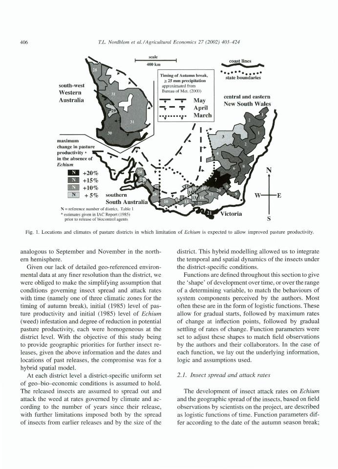
s Fig. I. Locations and climates of pasture districts in which limitation of Echium is expected to allow improved pasture productivity.

analogous to September and November in the north­ern hemisphere.

Given our lack of detailed geo-referenced environ­mental data at any finer resolution than the district, we were obliged to make the simplifying assumption that conditions governing insect spread and attack rates with time (namely one of three climatic zones for the timing of autumn break), initial (1985) level of pas­ture productivity and initial (1985) level of Echium (weed) infestation and degree of reduction in potential pasture productivity, each were homogeneous at the district level. With the objective of this study being to provide geographic priorities for further insect re­leases, given the above information and the dates and locations of past releases, the compromise was for a hybrid spatial model.

At each district level a district-specific uniform set of geo-bio-economic conditions is assumed to hold. The released insects are assumed to spread out and attack the weed at rates governed by climate and ac­cording to the number of years since their release, with further limitations imposed both by the spread of insects from earlier releases and by the size of the

district. This hybrid modelling allowed us to integrate the temporal and spatial dynamics of the insects under the district-specific conditions.

Functions are defined throughout this section to give the 'shape ' of development over time, or over the range of a determining variable, to match the behaviours of system components perceived by the authors. Most often these are in the form of logistic functions . These allow for gradual starts, followed by maximum rates of change at inflection points, followed by gradual settling of rates of change. Function parameters were set to adjust these shapes to match field observations by the authors and their collaborators. In the case of each function , we lay out the underlying information, logic and assumptions used.

2.1. insect spread and attack rates

The development of insect attack rates on Echium and the geographic spread of the insects, based on field observations by scientists on the project, are described as logistic functions of time. Function parameters dif­fer according to the date of the autumn season break;

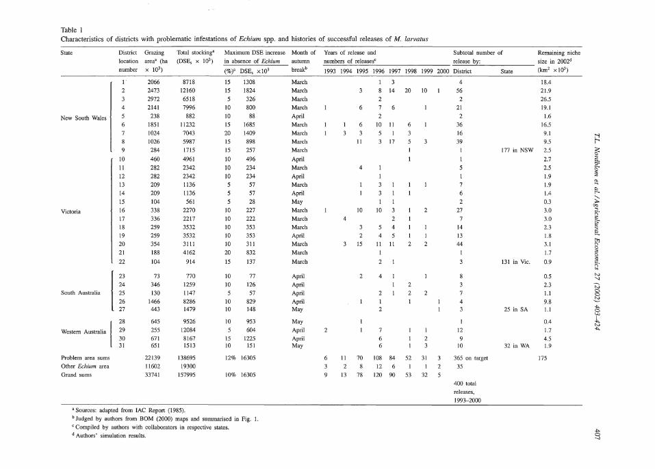
Table I Characteristics of districts with problematic infestations of Echium spp. and histories of successful releases of M. larvatus

State

New South Wales

Victoria

District Grazing

location area' (ha

number x 103)

I 2

4

5 6 7

8

9

10

II

12

13

14

15

16

17

18

19

20

21

22

24

2066

2473

2972

2141

238

1851

1024

1026

284

460

282

282

209

209

104

338

336

259

259

354

188

104

[

23

South Australia 25

73

346

130

1466 443

26 27

Western Australia 29 {

28

Problem area sums Other Echium area

Grand sums

30 31

645

255

671 651

22139

11602

33741

Total stocking'

(DSE, X 103 )

8718

12160

6518

7996

882

11232

7043

5987

1715

4961

2342

2342

1136

1136

561

2270

2217

3532

3532

3111

4162

914

770

1259

1147

8286 1479

9526

12084

8167 1513

138695

19300

157995

'Sources: adapted from lAC Report (1985).

Maximum DSE increase Month of

in absence of Echium autumn

(%)' DSE, x 10' breakb

15

15

5 10

10

15

20

15

15

10

10

10

5 10

10

10

10

10

20

15

10

10

5

10 10

10

15 10

1308

1824

326

800

88

1685

1409

898

257

496

234

234

57

57

28

227

222

353

353

311

832

137

77

126 57

829 148

953

604

1225 151

12% 16305

10% 16305

March

March

March

March

April

March

March

March

March

April

March

April

March

April

May

March

March

March

April

March

March

March

April

April

April

April May

May

April

April May

b Judged by authors from BOM (2000) maps and summarised in Fig. I.

' Compiled by authors with collaborators in respective states.

d Authors' simulation results.

Years of release and Subtotal number of Remaining niche

numbers of releases' release by: size in 2002d

1993 1994 1995 1996 1997 1998 1999 2000 District

2

6

9

4

6

6

II

4

10

2

15

2

11 70

2 8

13 78

I

8 14 20 10

2

7 6 2

10 11

5 17

10

2

4

4 5

11 11

2

4

2

2

7

6 6

6

I

2

2

2

2

2

2

2 3

108 84 52 31 3

12 6 I I 2

120 90 53 32 5

4

56

2

21

2

36

16

39

7

6

2

27

7

14

13

44

7

4

12

9 10

365 on target

35

400 total

releases,

1993-2000

State (km2 x103 )

18.4

21.9

26.5

19.1

1.6

16.5

9.1

9.5

177 in NSW 2.5

2.7

2.5

1.9

1.9

1.4

0.3

3.0

3.0

2.3

1.8

3.1

1.7

131 in Vic. 0.9

0.5

2.3

1.1

9.8 25 in SA 1.1

0.4

1.7

4.5 32 in WA 1.9

175

:-l J:-'

~ it "'"" ~ ~ ., ,..... :;: "" :::. " "' l! a ~ ;:,

~ ~-

"' 'l

-;:,

~ """

~

""" 0 _,

408 T.L. Nordblom et al./ Agricultural Economics 27 (2002) 403-424

both attack and spread rates are the highest with an early autumn break (March) and the lowest with a late break (May). This variation occurs because late breaks tend to decouple the occurrence synchrony of Echium and M. larvatus (Sheppard et al., 1999). The autumn break classifications were assigned to districts accord­ing to the month in which greater than 25 mm median rainfall is received, based on long-term monthly me­dian rainfall maps from the Bureau of Meteorology (BOM, 2000).

First consider a model of geographic spread:

S _ Ms t - 1 + eb,(I,-t)

(1)

where S1 is the rate of geographic spread of M. larvatus (kilometres per year) out from the release site in the tth year since release, see Fig. 3a, for which we assume: Ms is the maximum rate of geographic spread of M. larvatus in the particular autumn break region ( 1. 7 km per year for March, 1.0 for April and 0.8 for May); Is is the inflection year (the number of years from M. lar­vatus release at which the maximum increase in spread rate occurs: at 3 years where autumn break is in March, 5 for April and 10 for May); tis the number of years since M. larvatus was released at the release site; bs is the slope of the spread function at the inflection point.

Given the geo-referenced release date information provided by CSIRO collaborators in the various states and the timing of autumn breaks in the districts where releases were made, the maximum aggregated surface spread of each M. larvatus population was simulated. Results are plotted for the years 2010, 2020 and 2030 in schematic form in Fig. 2.

Our vision of the question of whether further re­leases of biocontrol agents might be economically justified and if so, "where and how many?", is embod­ied in our geo-referenced simulation results of Fig. 2 against the background of Fig. 1. The 400 releases made in the 1993-2000 period are expected to leave many gaps still in 2010, which close only slowly through 2020, 2030 and beyond. Answers for "how many?" are obviously not the same everywhere in the weed-infested parts of the country. This is not so obvi­ous simply from a look at the district data in Table 1. The characteristics of districts with the highest eco­nomic demand for new releases are combinations of too few earlier releases for the size of the potential for pasture recovery; that is, where there are large and

'·.

Western Australia

South Australia

s ~0 * Given the geo-referenced initial release dates and numbers (Table 1), and climatic factors (Figure 1), insect spread from release sites is simulated here for the years 2010, 2020 and 2030. In the current study we focus on the questions of where, and how many, further releases are economically justified to accelerate the spread and density of insect coverage of Echium beyond that depicted in this chart.

Fig. 2. Simulated maximum surface extent of only the 400 pop­ulations of biocontrol insects released against Echium in the 1993-2000 period.

costly gaps remaining in insect coverage. We have constructed a model to quantify the economic ques­tions of "where and how many?" and to show how the answers change with different pasture values, costs of new releases and discount rates.

In two-dimensional geographic space, we assume that M. larvatus spreads evenly in all directions out­ward from the release site. That is, in succeeding years the insect population spreads away from the re­lease site in concentric rings, ultimately with maxi­mum widths of 0.8-1.7 km each year (Ms. as defined earlier). Given the distance the insect spreads from a release site in t years (S1 ), we may estimate the surface area newly invaded in the tth year (N1) by subtracting the area of maximum reach of the insect in the prior year ( Jr s;_ 1) from that in the current year:

(2)

where 1r is the ratio of the circumference to the di­ameter of a circle, such that the area of a circle is 1r

times the square of the radius.

T.L. Nordblom et al./ Agricultural Economics 27 (2002) 403-424 409

The newly invaded area N1 is expressed in km2 of land surface. We label each ring (c) according to the time it was first invaded by M. larvatus. Therefore, the area of any of the concentric rings of land may be expressed as:

Nc = n(s;- s;_1) (3)

where Sc is the distance from the release site to the outer edge of concenuic ring 'c' following the defini­tion of S in Eq. (1).

"C C'll 2 (!) .... c. Ill

1.5 Ill~-::3' ... ~

~ ~ 1 ~ E ~

.lll:! - 0.5 -0 (!)

0 't;j

;

I I/ r

lj__j ....

0 10 20

"' .l!l ! 1: f. oOOOOOOOO

!!: .!!! 0.8 c.

.lll: 0 0 0.6 "' :::: 1:

"' :8 ... 0.4 0 0 Q) c. "' ~ .5 0.2

..9: 0

I o OL1'

J;J

}o 0 I

I o J;J

..L,~ 0 0 ',,rQ,,no

The idea of the cth concentric ring allows the ex­pression of insect attack rates on Echium as a function of ring position and elapsed time since release:

Ma Act = for c :::; t 1 + ehaUa-t+c)

(4)

where Act is the proportion of Echium plants in the cth concentric ring area attacked in the tth year since M. larvatus was released at the centre (release site), see Fig. 3b, for which we assume: Ma is the maximum

St (from Eq.l)

30 40

At (from Eq.4)

000000000 000000000 0000

March

April

May

March April

May

0 10 20 30 40

.lll: 600 0

ra "' 500 :::: Cll "' ... 400 ra >< Cll "'"'~ > E E 300 ~ ctS :::. 200 'S'C E ~ 100 ::I Q) (.) > 0 0

Q)

p . .& rJOo.~o

~I *0 ~'~u

-~' CZi 0 .,&.VJ ~ u

...... " () .;:/ ~0 ..... ~0 i

~'I ~ 1P I o'

-.nn2 • o 0 ~ ,nn[ oDu I . nnnnnnnnn, nn , 1 "' ,. ., 1 "'

0 0 10 20 30 40

years from release of M. /arvatus at a site

Fig. 3. M. larvatus spread and attack rates on Echium and cumulative areas covered at maximum attack rates, according to the timing of the autumn break (commencement of rains in March, April or May).

410 T.L. Nordblom et a!. I Agricultural Economics 27 (2002) 403-424

proportion of plants attacked by M. larvatus in the particular autumn break region (1.0 in March, 0.91 in April and 0.8 in May); Ia is the inflection year (the number of years of M. larvatus presence in an area at which the maximum increase in attack rate occurs: 5 years where autumn break is in March, 7 for April and 10 for May); and ba is the slope of the attack function at the inflection point.

Our concentric rings vary in width, being very nar­row in the first years from release (see Fig. 3a), grow­ing in width as a logistic function of time . . . and stabilising at a maximum rate in kilometres per year determined by climatic zone. Likewise, we assume in­sect densities, or attack rates, increase at a given spot as a logistic function of time (see Fig. 3b), eventually reaching a maximum determined by climatic zone. Only three such zones are defined in the model, reflect­ing again our lack of detailed information on insect response, but also our desire to account for observed differences in spread and attack rates in different parts of the country.

Combining the attack and spread functions in a simulation model allows prediction of surface areas

5 years

0 5

covered by insects at different densities over time. Thus, with the combined effects of Eqs. (1) and (4), the area (krn2) covered by M. larvatus at a particular attack density will increase exponentially with time, most rapidly in regions with early autumn breaks and most slowly with late autumn breaks (Fig. 3c).

Only our insect release date and location data are gee-referenced by Lat/Long, but this is overlayed by climatic zone information at the district level, which is used to calculate the geographic spread of each released population over time. For three future dates (2010, 2020 and 2030) the simulated geographic extents of each of the 400 populations, depicted by growing dot-sizes, were plotted with a mapping program according to their Lat/Long coordinates to produce Fig. 2. This image fairly illustrates the geographic scatter of release sites, the presence of gaps between the growing peripheries of the result­ing populations and their eventual merging in some areas with remaining gaps elsewhere. What Fig. 2 does not show are the insect-density distributions as­sociated with each release, as schematically shown in Fig. 4. Nor does it indicate any of the economic

8 years

km

10 15 20

11 years

* Four sites with releases made 5, 8, 11 and 14 years in the past, in a region with autumn breaks in April

Fig. 4. Schematic map of sequential geographic spread of M. larvatus on Echium at four different sites.

T.L. Nordblom et al. I Agricultural Economics 27 (2002) 403-424 411

consequences, which are derived with our spreadsheet models that operate on a district level into which the geo-referenced release date information were allo­cated. These models account for pasture productivity gains, the value of these gains, the costs of new re­leases and limits to the values of new releases due to district size and interference by populations released in the past as well as the number of new releases.

At any point in time after the year of release of M. larvatus, the areas closest to the release site are assumed to have greater attack rates than areas fur­ther from the release site (Fig. 4). A sequence of geo­graphic spread and increasing attack rates, at 5, 8, 11 and 14 years from release, is illustrated in this figure for a region with autumn breaks in April.

Insect releases against Echium are distributed spa­tially within a district such that the resulting popu­lations may have no contact with one another until they have spread for many years. We assume a newly released population's geographic coverage grows as the square of the radius from the release site to the outer periphery of the population and the growth in the length of this radius itself is a logistic function of time. For example, in an area with autumn breaks in April, the maximum spread from a release site in 5 years, would have a radius of just 0.96 km and cover only 2.9 km2 . At 10 years, we assume the ra­dius grows to 5.5 km from the release site for a max­imum geographic extent of 95 km2. At 20 years the radius reaches 15.5 km for a maximum compass of 7 54 km2 ; at 30 years the radius is at 25.5 km, covering 2042 km2 and so on. Thus, the area increases expo­nentially, slowly in the first years from release, then rapidly as a steady maximum rate of growth of the radius is reached.

Attack rates by the biocontrol agents are also as­sumed to build up slowly at first, then more rapidly toward a maximum at any spot in the given climatic zone, depending on the number of years the biocontrol agent has been at that spot (as illustrated in Fig. 4). The integral expressing the total area attacked at max­imum rates (for the climatic zone) likewise increases exponentially with the square of the radius (Fig. 3c). Typically, where there have been scattered releases across a sub-district, their attack integrals are summed together each calendar year in our model and these are aggregated up to the district level for a sequence of attack levels.

For the cases of releases in regions with earlier or later autumn breaks, March or May, the geographic spread is assumed to be greater or smaller, respectively and the parameters M8 and /8 in Eq. (1) are set accord­ingly. This simulation is an abstraction from a more complex reality in which heterogeneous environments surrounding each of the 400 release sites would warp the picture in its own unique way. Our severe data limitations made it impossible to depict local envi­ronmental obstacles, which we know must be present. In effect, however, we have implicitly assumed dis­trict boundaries are insurmountable obstacles to the insects, a countervailing simplification. Here, we have a rough way to account for time since release and for relative environments (month of autumn break) in simulations of geographic spread and development of attack rates. This sets the stage for the next step in our analysis.

It was assumed for districts in which there was more than one release, the maximum spread of insects from each release was to the area defined as the district to­tal divided by the number of releases in the district. This is a conservative assumption given the fact that the earliest insect releases (say in 1993 versus 2000) will have spread over greater surface areas and reached greater densities than later releases and the fact that insects are not really limited by administrative bound­aries. These conservative assumptions were made to limit the computational burden posed by 400 insect re­leases distributed over an 8-year period across 44 dis­tricts of varying size. In our model, the 400 releases and 44 districts define 130 sub-districts, depending on year of release, for which year-by-year sequences of areas with partial relief were simulated. These are ag­gregated back to the 44 districts as area equivalents with full economic loss relief.

There are several other conservative assumptions in our analysis. While our model implies all long-term biocontrol of Echium will result only from the activ­ity of M. larvatus, the crown weevil, there is good reason to anticipate complementary successes of the other agents released against the weed. Nordblom et al. (2001) conservatively assumed no further re­leases beyond the 400 successful establishments; in reality, state departments of agriculture will continue to respond to farmers' requests (Shepherd, 1993) and Australian Wool Innovation and Meat and Livestock Australia continue important support for releases of

412 T.L. Nordblom et al./ Agricultural Economics 27 (2002) 403-424

biocontrol agents against Echium. Also, the model focuses on the valuation of increased pasture produc­tivity and ignores reductions in conventional spraying costs which formed a significant share of the antic­ipated benefits calculated in the lAC Report (1985) and that of CSIRO (1998). While reductions in pas­ture spray costs may be anticipated, these are likely to be replaced with the costs of measures taken by farm­ers to facilitate the success of the biocontrol agents and to limit reinvasion by other pasture weeds (Taylor and Sindal, 2000; Auld, personal communication, 2001). The model also ignores control costs and losses attributable to Echium as a weed in crops; these amount only to some $1.2 million annually (Jones et al., 2000) and may be assumed to continue indefinitely.

While conveniently concentric, our expansion rings of insect population are not at all evenly spaced or of constant width, until a number of years after re­lease when the rate of growth of the radius stabilises. The need for us to explicitly model the space, time, insect-density dynamic (expressed in Eqs. (1) and (4) and Fig. 4 ), arose when we were faced by field obser­vations that differed across the country due to climatic influences on the insect and the host weed. Individual treatment of sub-districts with unique release dates, otherwise homogeneous in conditions within the dis­trict and heterogeneous across districts, allowed indi­vidual modelling of each insect cohort from multiple releases across different years in the 1993-2000 pe­riod and possible new releases in 2002.

2.2. Expected relief due to past insect releases of economic losses caused by Echium

The relations between attack rates (Act) and relief of economic loss caused by Echium in pastures are sim­ulated on the basis of several assumptions. First, we assume there will be no beneficial effect from attack rates below 50% of Echium plants. Second, we assume that even with 100% of Echium plants being attacked by M. larvatus, a maximum of 90% reduction in eco­nomic loss is possible. Third, we assume economic loss reduction increases at increasing rates as attack rates rise, up to an inflection point at Act = 85%, thereafter increasing at decreasing rates to the max­imum of 90% loss reduction at Act = 100%. These assumptions are captured in Eq. (5).

(5)

where Ret is the proportion of pasture productivity loss reduction in the cth concentric ring area due to the attack rate (Act) expected in the tth year since M.

larvatus was released at the centre (release site), for which we assume: M R is the maximum proportion of pasture loss reduction achievable, 0.9 in a March au­tumn break region where 100% attack rates are pos­sible; lR is the inflection point (taken to be the attack rate, Act = 85%, at which the maximum increase in loss reduction occurs), this is assumed to hold in all regions; bR is the slope coefficient of the loss reduc­tion function at the inflection point; Act from Eq. (4), is the proportion of Echium plants in the cth concen­tric ring area attacked in the tth year since M. larvatus was released at the centre (release site).

For the April and May autumn break regions, where maximum attack rates are assumed to be 90 and 80% respectively, the maximum proportions of pasture pro~ ductivity loss reduction are taken to be 0.68 and 0.32 (Fig. 5).

In approaching measures of economic loss caused by Echium, we relied on a combination of indicators from the lAC Report of 1985. The first of these was a table of local estimates, by district, of the maximum

~

1l 0::

"0 Q) > .!!! ~ 1/1 1/1

..!2 1.) .E 0 c: 0 1.) Q)

0 c: 0 :e 0 c. 0 ... D.

0.9

0.8

0.7

0.6

0.5

0.4

0.3

0.2

0.1

--------------,

----------------Max for autumn break in April

I I

0+-~--~~----~~--~~~~~ 0.0 0.1 0.2 0.3 0.4 0.5 0.6 0.7 0.8 0.9 1.0

Proportion of Echium plants attacked (Act)

Fig. 5. Proportion of pasture productivity loss recovered as a func­tion of the proportion of Echium plants attacked by M. larvatus.

T.L. Nordblom et al. I Agricultural Economics 27 (2002) 403-424 413

proportion of pasture productivity gain expected with the total absence of Echium. These estimates ranged from +20 to -10%. That is, in removing the worst cases of Echium infestation, only a 20% improvement in pasture productivity was expected (Fig. 1, Table 1). In the few cases where Echium was thought to provide a positive contribution to productivity, its total removal was expected to cause a maximum net reduction of 10% in pasture productivity. In those parts of South Australia (not shown) Echium is known as 'Salvation Jane'.

The second of the indicators was the number of grazing livestock present in each of the regions. Ag­gregate stocking numbers in each district are expressed as 'dry sheep equivalents' (DSE) where 1 DSE relates to the feed requirements of one wool sheep, 1.5 DSE represents a meat sheep, 10 DSE a beef animal and 15 DSE a dairy cow. Finally, estimates of pasture ar­eas in each district were given in the 1985 lAC Report (Table 1).

One can think of DSE units as a measures of pasture productivity that may be aggregated across a district, such that:

DSE0 = l.OWOOL + 1.5MEAT

+10BEEF + 15DAIRY (6)

where DSEo is the number of DSE units in a district, based on the conversion factors discussed above for the four classes of grazing livestock.

The 400 successful releases of M. larvatus were made at known dates and locations across southern Australia from 1993 to 2000. About 91% of these past releases were concentrated in districts where Echium is considered economically damaging (Table 1). For simulation purposes, as mentioned earlier, it was as­sumed for each district in which there was more than one release, the maximum spread of insects from each release was to an area defined as the district total divided by the number of releases in the dis­trict (RELEASESo). For each of these single-release sub-districts, we assume DSEo is also equally allo­cated. Thus:

AREA0 (km2) AREAct = RELEASESo (7)

and

DSE = DSEo (number of DSE units) (8) d RELEASESo

where the subscript 'D' indicates district level and 'd' indicates single-release sub-district level.

We multiplied two of the lAC Report indicators, maximum percentage productivity change in absence of Echium (assumed to hold equally at district and sub-district levels) and DSEct, to derive estimates of the maximum change in stocking in the absence of Echium.

max ~DSEct = (MPPCct) (DSEct) (9)

where max ~DSEct is the theoretical maximum change in pasture productivity in absence of Echium, mea­sured in DSE units (see Table 1 where only the 31 districts with significant loss recovery potentials are shown); MPPCct is the maximum proportional change in pasture productivity in the absence of Echium in the sub-district, derived for each district in local work­shops as recorded in the lAC Report (1985); DSEct is the total stocking in sub-district 'd' as defined in Eq. (8), derived from the lAC Report (1985) for each of the districts.

We assume that eradication of Echium is unattain­able with M. larvatus, though strong limitation of the weed by this biocontrol agent has been observed under favourable conditions. It is the year-by-year progress of the agent toward the locally attainable lev­els of weed limitation that we may now simulate at the sub-district level. As described under Eq. (5), maxi­mum reductions in economic loss are assumed to be limited to 90, 68 and 32% in areas with autumn breaks in March, April and May, respectively, due to limits on attack rates and/or limits on the efficacy of the agent.

Because of the progressive spread and increase in attack rates of M. larvatus with time (Fig. 4), we may consider both of these dimensions in a formula that integrates the status of all the concentric rings about a release site in sub-district 'd' at a particular moment in time (year t) in terms of total recovered pasture productivity in a sub-district (Eq. (10)).

max ~DSEctL~=l (RctctNctc) RDSEctt = (10)

AREAct

where RDSEctt is the weighted total increase in DSE units from the 1985 baseline prior to release of M. larvatus in sub-district 'd' as of year t, in DSE units; we call these "recovered DSE8"; max ~DSEct is the maximum change in stocking in the absence of Echium; this is taken as an unattainable theoretical

414 T.L. Nordblom et al./ Agricultural Economics 27 (2002) 403-424

measure of potential pasture productivity change in sub-district 'd', in DSE units, as defined in Eq. (9); Rctct is the proportion of pasture productivity loss reduction in the cth concentric ring area (Eq. (5)) due to the attack rate (Act) expected in the tth year since M. larvatus was released in sub-district d; Nctc

is the area of a concentric ring of land in sub-district 'd' invaded by M. larvatus (Eq. (3)); this serves as a weighting numerator in the formula; AREAct is the area of sub-district 'd', in km2 , as defined in Eq. (7), used here as the weighting denominator.

The 400 releases distributed among the 8 years and 44 districts defined 130 sub-districts, depending on year of release, for which year-by-year sequences of areas with partial relief were simulated. The sequence of aggregate change in pasture productivity, or 'recov­ered DSEs' (RDSEct) was calculated at the sub-district level given the simulated areas of spreading concen­tric rings and the attack densities in each of them at a given time since release. Thus, RDSEct was simulated with Eq. (10) on a year-by-year basis from 1993 to

60 , un-discounted I

I I values, based on I

50 I $8 DSEs r:: I

g I I

I state I

E I 40

* I ----·NSW I

ti I -VIC I - I :;: I -+-SA Q) 30 I

r:: Q) -WA .c ctS :::J 20 r:: r:: ctS

10

0 0 "' 0 "' 0 Kl 0 ~ 0 "' 0 0 0 C\l "'

..,. ..,. 0 0 0 0 0 0 0 0 0 C\l C\l C\l C\l C\l C\l C\l C\l C\l C\l

0

"' 0 C\l

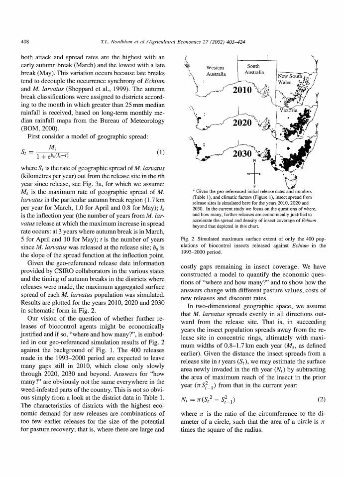
2050 for each of the 130 sub-districts with successful releases between 1993 and 2000. The RDSEct results were then aggregated up to district, state and national levels as calendar sequences over the same years.

In order to express the aggregate economic relief due to the past 400 releases in dollar terms a conser­vative value per recovered DSE is wanted. We have taken $8/DSE as the low end and $16 as the high end of a conservative range of values for recovered pas­ture productivity. Values at the high end are typical for sheep and cattle enterprises in NSW, where the greatest infestations of Echium occur. The year-by-year esti­mates of dollar value loss relief were aggregated across districts by state. The simulated time paths of these benefits for each state are given in Fig. 6. The great­est benefits from biocontrol of Echium are anticipated in NSW, followed by Victoria and Western Australia. Comparatively smaller benefits are expected for West­ern Australia and South Australia, where there have been fewer successful releases and where the late au­tumn breaks put M. larvatus at a disadvantage.

20

r\ 18 I \

I \ discounted I \ 18 I \ values, at

I \ r = 0.1 (10%) \ \ 14 I \ \ \

12 I

\ ' 10

\

\ I

8 \ \

8

4

2

0

year

Fig. 6. State-by-state benefits of past releases (1993-2000).

T.L. Nordblom et al./ Agricultural Economics 27 (2002) 403--424 415

For a given sub-district, with a single-release date (t = 0), the present value (PV) would grow expo­nentially with the geographic coverage and density of the insect population until the insects fill the available niche of Echium in, say, n years:

PV = ~ (PnsE)(RDSEctt) :S;' (1 + r) 1

(11)

where PV is the discounted potential present value of a newly released biocontrol agent; RDSEct1 is the expected amount of 'recovered DSEs' of pasture loss in year t, as defined in Eq. (10); PosE is the dollar value expected per unit of 'recovered DSE'; and r is the discount rate for relating future benefits to present values.

The discounted net present value (NPV) of the biocontrol program that organised, enabled and im­plemented the releases of insects in the 1993-2000 period is calculated to be on the order of $410 million as of 2002 (Nordblom et al., 2002), over the period of 1972-2050, assuming a value of $8 per recovered DSE and a discount rate of 10% (Eq. (12)).

NPVpast =I t ~ (l ~ r~2~o02J state= I i = 1972

= $410million (12)

where NPV past is the expected net present value of the past program of research, development and release of biocontrol insects against Echium from 1972 to 2050, state refers, in turn, to New South Wales (NSW), Victoria (VIC), South Australia (SA) and Western Australia (WA), Bi is the sum of state-wide benefits of biocontrol of Echium in year i, from 2000 to 2050 and C is sum of state-wide costs in year i, including shares of the national expenditures, for development and implementation of the biocontrol program from 1972 to 2000.

While $410 million may be quite a respectable amount, considering the accumulated costs of the biocontrol program from 1972 to date have been on the order of $14 million and the benefits only began to accrue since about 2000, it provides no informa­tion on what to do next beyond the general message: 'biocontrol programs are good investments'. The very gradual expected increases in benefits (panel 'a' of Fig. 6) and the 'spottiness' of coverage from these

past releases (Fig. 2), give rise to questions of where and how many further releases of insects might be justified against Echium.

2.3. Thirty-one diminishing niches for further releases

Of the 44 districts where M. larvatus populations have been successfully established in the 1993-2000 period, 31 are identified as candidates for possible fu­ture releases. These are the ones listed in Table 1 and depicted in Fig. 1. The criterion for this is the expecta­tion that harmful concentrations of Echium still exist in pastures of these districts, based on the original 1985 lAC Report. Thus, we exclude from consideration 12 districts where insects had been released on Echium infestations thought to be causing little or no economic loss and one district in South Australia where Echium was considered a positive contributor to pasture value. Our interest here, however, is in those districts where Echium is associated with important economic losses in pasture productivity.

Given the fact that M. larvatus populations have already been established in each of these 31 districts and that each of those 400 populations is thought to be expanding, the niches for capturing benefits with further insect releases must diminish with time. To avoid any double-counting of benefits, there is a need to quantify both the spatial and temporal di­mensions of the remaining niches for any further new releases of insects to contribute toward more rapid limitation of Echium. The pace of diminishment of the niche for new releases will vary from district to district depending on the number and timing of past releases as well as district size and climate. Simula­tions of the diminishing niche and potentials for new releases were plotted for a large April break district (Fig. 7).

For example, 10 new releases in a 9300 km2 dis­trict (Fig. 7) are expected to contribute the equivalent of complete control of Echium on some 1200 km2 by about the year 2025. Thirty new releases would be ex­pected to control Echium on about 2200 km2 by about 2023 and 100 new releases would cover 3000 km2 by 2021. These peak benefits, attributed to new releases, would be expected to diminish beyond these dates due to the still-expanding populations of insects released in the 1993-2000 period. As the populations merge, we

416 T.L. Nordblom et al.l Agricultural Economics 27 (2002) 403-424

10000 ~--------------------------------------------, New releases in 2002

Total April break area 9000

-+-10 8000 +-------------------------------------------~

-A-- 20

7000 +-------------------------------------------~ -f:r- 30 maximJm area equivalent with full relief (68% for April break)

N

E .¥ ai 5000 +--------------------____;)--... ~ cu 4000 +-----------------------~

8 '<t

0 <D

0 a>

0 N N N N

0 g.: N

expected relief of pasture losses due to insects released in the 1993-2000 period

-o- 50

~100

""*'"Past

Fig. 7. Schematic example of the diminishing niche for new releases in a district and expected effects of new releases in 2002.

must not double-count their benefits. Maximum attain­able benefits in a district are simply achieved several years earlier with the new releases than without them.

We define a 'limit function', keyed to the size of the niche in the year 2002 (ranging from 300 to 26,500 km2) for new releases in each district, to progressively reduce the marginal contribution of additional new releases in a given niche. This is to further reduce the possibility of double-counting of anticipated benefits by allowing for stronger competi­tion with the fact that the final new releases will have less scope for free expansion than the first new re­leases. These are limits in addition to those imposed by the 'diminishing niche' affect of releases in the 1993-2000 period. Thus, we have:

1 L = 1 - ----,,...,..,.,...,...,..-__,..,.

1 + e (b((k fd)- x+s)) (13)

where L is a limit, being the proportion of free expan­sion allowed to the marginal insect population released in a district in 2002; k is the estimated total size of the niche for new releases in a district in 2002 (km2); d is a common divisor (km2) determining the inflection point number of releases; sis a shift constant (km2) for

the inflection point number of releases; b is the slope of the limitfunction at inflection; and x is the number of releases at which the marginal release is considered.

The effect of the 'limit function ' (Eq. (13)) for a given niche size is to allow almost free expansion to the first proportion of new releases, greater restrictions on the expansion pace of the next portion of releases and severe limits on expansion of any further new releases (Fig. 8).

Costs of scouting release sites are implicitly in­cluded in our 'cost per release' values of $2000 or 1000 ($2K or $1K). These two scenarios of marginal cost per release, in addition to covering the costs of scouting potential release sites, include the costs of contacting willing landholders who are able to help set up and protect insect cages in their Echium patches and monitoring the process. Local scouting and intelligence at the district level allows placing new insect releases in weed-infested sites where previously-released populations have not yet reached. Investments in such purposeful local scouting are considered likely to have higher payoffs than invest­ments in higher resolution data and simulation at this stage.

T.L. Nordblom et al.! Agricultural Economics 27 (2002) 403-424 417

Q) tn 0 Q) Ill tn c.«< c:: Q) o­'iii !!:! c:: Q)

[:E; ~a; 'C ·= $~ ·- Ill ,§ E c:: Q) ::s..s:::: --o.s r::::'C 0 Q) t: c:: 0 .!2> C.tn 0 tn Q.lll

1.0

0.9

0.8

0.7

0.6 -

0.5 -

0.4

0.3

0.2

0.1

niche size (km2)

-<>- 300 --ir 6300 -D-12300 -o-18300

number of new insect population releases in 2002 after marginal five are added

Fig. 8. Limit function reducing the pace of expansion of a marginal five releases, for a new total of releases in 2002, given the size of the remaining niche in a district.

For each of the 31 districts, simulated effects of new releases of insects in 2002 were traced for the 2002-2050 period, in 20 increments of five releases (up to 100). These runs calculated marginal RDSEct1

values for each year (as in Eq. (10)) and the PV (as in Eq. (11) for given DSE values and discount rates) for each of the 620 ( = 31 x 20) district/release-level combinations, limited by the year-specific niche size for the district and by Eq. (13) on the pace of ex­pansion of marginal releases, keyed to calculated niche size in 2002 (Table 1). The PVs of the 620 district/release-level combinations were then sorted from the highest to lowest.

3. Results and discussion

The cumulative PV results for three combinations of DSE value/discount rate are plotted as cumulative values in Fig. 9: (a) $16 DSE/5% discount rate, (b) $12 DSE/10% discount rate and (c) $8 DSE/15% discount rate. Only the cumulative PVs of the best 1500 of the 3100 (= 620 x 5) releases are plotted. In the most favourable economic scenario (a) total PV of benefits

could exceed $100 million for a new release project. In the least favourable condition (c) the total PV of benefits would not exceed $9 million. The more mod­erate middle scenario (b) indicates total PV s above $25 million for a new release project.

Under each of the three economic scenarios (a-c in Fig. 9) national NPVs were calculated for different total numbers of new releases for the cases of marginal costs (MC) of $1000 and 2000 per release.

NPVn = PVn- nMC (14)

where NPVn is the expected net present value of n

new releases given that PV n is the discounted present value of n new releases according to Eq. (11) at the district level and ranked across all districts and states from the highest to lowest PV and nMC is the number of new releases in 2002 times the marginal cost per release.

The numbers of releases at which NPV n is max­imised are indicated for each case by a vertical line and corresponding numerical value (Fig. 9). Likewise for the objective of marginal benefit:cost ratios exceed­ing five (MBCR > 5), an investment criteria aimed at avoiding low-benefit releases.

418 T.L. Nordblom et a!. I Agricultural Economics 27 (2002) 403-424

Fig. 9. National project optimisation for releases in 2002 under 12 economic scenarios. Three combinations of DSE value and discount rate (a, b and c) and assuming basic fixed cost of project at $1 million and objectives of maximising net present value (NPV) or limiting priority releases to those expected to yield marginal benefits in excess of release costs by a ratio of at least 5 (MBCR > 5), given marginal costs of $1000 or 2000 per release.

For illustrative purposes, we point to a middle sce­nario we call "X" in Fig. 9. This assumes $12 DSE8 ,

a 10% discount rate, $2K release costs and, with its objective of MBCR > 5, calls for 410 total new re­leases. This scenario is identified in Figs. 10-12 and is the subject of Fig. 13.

A sensitivity analysis with 18 economic scenarios, defined by three discount rates (5, 10 and 15%), three DSE values ($8, 12 and 16) and two marginal costs per release ($1K and $2K), was completed for each of the two national project objectives: (a) maximum NPVn and (b) MBCR > 5. Results for the 36 cases

are given in terms of optimal total number of releases in 2002 (Fig. 10) and expected national project bene­fit:cost ratios (Fig. 11). In every case, the more restric­tive investment criteria of MBCR > 5 calls for lower numbers of new releases than the NPV n -maximising objective (Fig. 10). As expected for the criteria that avoids low-benefit releases (MBCR > 5), project benefit-cost ratios are higher in every case than with NPV n-maximisation (Fig. 11).

It is most likely that a national project for new releases would aim to maximise investment returns while avoiding low-benefit releases. This is because

T.L. Nordblom et al. I Agricultural Economics 27 (2002) 403-424 419

(a)

1400

0 m 12oo ..Q~ § ~ 1000 c .E Cl 800 .5 lll .!!! :g 600 E Q) ")( ~ lllE 3: 400 ' Q) ii: c 200

z 0 '-----

--<>-5%

-D-10%

(b) 1000 -,---------,.

Ill It) 900

5! AI 800 lila: ..!!! (.) 700 ~m 3: :a soo ~ 1ii 500 - -Q) 0 ... Q)

..Q

E ::I c

"iU -0 1-

Ill

> -·;: 0 ·;: c. J: -"i

400

300

200

100

0

Cost of each new release = $2k

discount rate L ______ _,

$8 $12 $16 $8 $12 $16 Value of added pasture productivity($/ DSE)

Fig. 10. Optimal total number of new releases in 2002 under 36 scenarios. Scenarios comprise combinations of two costs of each new release, three discount rates, three values of recovered pasture productivity and two project objectives, (a) maximising net present value (NPV) or (b) limiting priority release to those expected to yield marginal benefits in excess of release costs by a ratio of at least 5 (MBCR > 5).

such a project would need to be supported in full by the grazing industries that are most likely to benefit from it. Therefore, we present district-by-district op­timal numbers of releases in 2002 only for the case of the investment criteria, MBCR > 5 (Fig. 12). These were calculated for the same three combinations of DSE value and discount rate, (a) $16/5%, (b) $12/10% and (c) $8/15% and two marginal costs per release ($1K and $2K), for which total numbers of releases are listed at the bottom of Fig. 9 for MBCR > 5. As in the case of total numbers, the optimal releases are never greater at the district level with marginal release

costs at $2K than at $1K. They are sometimes equal in our analysis because the five-release increments we used are so large. However, if we had considered single-release increments instead, equal numbers of releases with $1K and $2K marginal costs would be rare indeed, except for districts where even the lower cost exceeds a fifth of the expected benefit; that is, the cases where no releases are called for by the MBCR > 5 criteria.

What is evident in the district-by-district results is the considerable number of districts for which no, or very few, new releases are called for (Fig. 12).

420 T.L. Nordblom et al.! Agricultural Economics 27 (2002) 403-424

(a)

~ Ill E Q) I tfl

>tiS fl.. Q) ZQj .... ....

.e 3: 0 Q) ·- 1: -ta-.... 0 u Ill m a; -..o l§ 0 1: .... fl..

(b)

~1.1) 0 AI ·;: a: a.u :Sm "§: ~ o1Q

+= ..... tiS Q) .... Ill u Ill • • Q) m 111 - tiS u Q) Q)-·- Q) 0 .... .... fl..

45

40

35

30

25

20

15

10

5

0

55.0 50.0 45.0 40.0 35.0 30.0 25.0 20.0 15.0 10.0 5.0

Cost of each new release = $1 k

Cost of each new release = $2k

-<>-5%t -D- 1 O% discou t rate· ·

-!:r-15% ..

0.0 -+------;------4

$8 $12 $16 $8 $12 $16

Value of added pasture productivity($/ DSE)

Fig. 11. National project benefit-cost ratios expected in 2002 under 36 scenarios assuming a basic fixed project cost of $1 million in addition to release costs. Scenarios comprise combinations of two costs of each new release, three discount rates, three values of recovered pasture productivity and two project objectives, (a) maximising net present value (NPV) or (b) limiting priority release to those expected to yield marginal benefits in excess of release costs by a ratio of at least 5 (MBCR > 5).

In the case of a few districts, however, rather large numbers of new releases are called for, even in the least favourable economic setting (panel c, with $2K marginal costs). These few provide targets and answer the questions of 'how many and where' new releases are justified economically. Another point worth not­ing in Fig. 12 is that the changes in optimal releases from one scenario to another are not proportional among the districts. This is due to the conditions of

the various districts being so different regarding dis­trict areas, pasture productivities, Echium infestation levels, climates and histories of past releases (recall Fig. 1 and Table 1).

Results of our middle scenario "X" (Figs. 9-12) are plotted for a clearer geographic perspective in Fig. 13, in which only 17 of the 31 districts would receive new insect releases. The numbers of releases in each of the 17 districts is also indicated.

I iii c

100 90 80 70 60

T.L. Nordblom et al./ Agricultural Economics 27 (2002) 403-424

• 0_ - - - - - -a. $16 DSE value and 5% discount rate • 0 ·o- : : : : : : : : :O: :0: : : : : -- _ -® __ : : : - - - - - - Q

--------------------------- ---0---- ()---"2' 50 ca 40 E 30 · c ca .c

- - - - - - Q- - - - - - - Qo®- - . - .• - - -Q ~ ®- -20 . - - - 0 - - - - - - - - - -0- - - - - - - - - -0- - . 0 - . - - - - . Q 1 ~~--~·~·~Q~-~~~~·-@~Q.· ~-.--~Q~-~·-Q~~~@rQ~--·~-~--Q.~-~·~@r·~-~·--~~~~ -

I C)

~ 100 ;; 90 Ll) 80 1ii 70

0 1 2 3 4 56 7 8 910111213141516171819202122232425262728293031

· - - - b. $12 DSE value and 10% discount rate - - - - -

n- ----- -- - ( solid dots in this panel comprise scenario ·x· )

~ 60-¥ 0

Q -.-- - -· 't;j

:1 ~ ~ iii c "2' ca E :S "i

50 40 30 20 10

N 100 8 90 N .E 80

70 60 50 40 30 20 10 0

• • • • • • • • ••• ~~· Q •••• o o ? • ? ••• 0 ®Q

0 1 2 3

- - - - - - - - - - - c. $8 DSE value and 15% discount rate - - - - - -

-- - - - - - -- o $1 k/ release -() - - - - - - · - - - - - - - - • $2k I release - - · - - - - · - - - - - -------------------------------------0------

.- ·o .-------.-------- -·---- 0

. - _@_-------.-- -·· 0 ·-0--· ----.------.-------- ·o----

0 1 2 3 4 56 7 8 910111213141516171819202122232425262728293031

District (see Fig. 1. for locations)

421

Fig. 12. District-by-district optimisation of new releases in 2002 under six economic scenarios. Assuming project objectives are to maximise benefits while limiting priority releases to those expected to yield marginal benefits in excess of release costs by a ratio of at least 5 (MBCR > 5).

Of course, there is no objective way to know which of the scenarios depicts the future better than the oth­ers. Optimal new release numbers of the 18 scenarios (Fig. 10), under each of the two project objectives ex­hibit a significant spread, from roughly half to roughly quadruple the number of successful releases made ear­lier in the 1993-2000 period. And, while the project

benefit-cost ratios for new releases (Fig. 11) are com­parable with those of other opportunities faced by the Australian grazing industries, they do not tell us pre­cisely what should be done. The clearest answers to the questions of 'where and how many' are provided in the district-by-district results (Fig. 12) that show across a range of economic conditions some districts

422 T.L. Nordblom et al.l Agricultural Economics 27 (2002) 403-424

south-west Western Australia

Optimal locations of 410 new releases in 2002, costing $2K each, given priorities for MBCR ~ 5, with $12/DSE values and

coast lines "r:w:s 5"? ~ ............

state boundaries

scale

400km

s

. • . • . central and eastern

New South Wales

Fig. 13. Example of optimally targeted numbers of insect populations for release in 2002: economic scenario 'X'. Note: small numbers indicate optimal number of release in 2002 in particular districts under scenario X (depicted at the district-by-district level in Fig. 12 and at the national level in Figs. 9, 10 and 11). The districts calling for large numbers of new releases are those with large potential gains from recovered pasture productivity (Fig. 1) and relatively few prior releases (Table 1).

consistently calling for large numbers of new releases and others calling for none or very few.

4. Conclusions

Our need to depict over a long sequence of years the annual sums in individual districts the effects of multiple releases of insects over time, led us to de­velop a model that takes into account different levels of geographic spread and development of attack rates on the host weed as functions of time since release and the climatic zone. The model allowed us to gain the nation-wide strategic view of geographic priorities for release action this year. In the results of the current model these priorities stand out boldly. The present analysis has gone some way toward answering the questions of where and how many additional targeted insect releases against Echium are justified beyond the 400 successful ones achieved in the past decade.

In order to enhance confidence in these modelling results, field monitoring work is required to test and correct the current assumptions on rates of geographic

spread of insects, rates of attack and rates of eco­nomic relief from suppression of Echium, under the different climatic regimes in the weed's range. These three rates are not only functions of climate, but may be reduced locally by inappropriate management practices of graziers/farmers. It is through this con­nection that the value of extension programs may be quantitatively estimated. Such monitoring, modelling and extension work is in the interest of the grazing industry groups who stand to benefit most. The clear indication of our present analysis, however, is that at fairly modest cost a new round of well-targeted insect releases against Echium will provide very respectable economic benefits.

Our explicit accounting for the spatial and temporal dimensions has made this economically optimal tar­geting of new insect releases possible. Legner (2002), Zeddies et al. (2001) and Coombs et al. (2000) have noted that complete economic analysis of biocon­trol projects are rare. Other studies have attempted benefit-cost analysis of biocontrol programs, but none we are aware of have treated the question of how many further releases of agents are justified economi-

T.L. Nordblom et al./ Agricultural Economics 27 (2002) 403-424 423

cally and none have done so in a spatial-bio-economic framework as does the present study. We hope this analysis facilitates such work by others, providing insights for tackling problems in natural resource management that develop, or whose amelioration develops, slowly over time and differentially over space.

Acknowledgements

We wish to thank David Vincent and David Pearce at the Centre for International Economics, Canberra (CIE), for raising a number of important questions over the course of our earlier analysis. We are also grateful to Bruce Auld and David Vere, NSW Agricul­ture, for useful critical comments. We thank those col­laborating at the state level with CSIRO-Entomology in the release and monitoring of biocontrol agents on Echium; in particular, those who provided the geo-referenced release location and date information required for this analysis: Kerry Roberts, Agriculture Victoria, KTRI, Frankston; Ross Stanger, SARDI, Entomology Unit, Adelaide; Paul Sullivan, NSW Agriculture, Tamworth; and Paul Wilson, Agriculture WA, South Perth. Funding support for such work from Australian Wool Innovation and Meat and Live­stock Australia is also gratefully acknowledged. The authors also gratefully acknowledge the helpful com­ments of the editor and two anonymous reviewers. Any errors found in this analysis, or opinions ex­pressed, are those of the authors and do not necessarily represent the policies or opinions of their respective institutions.

References

Auld, B., 2001. Orange Agricultural Institute, NSW Agriculture, Forest Road, Orange, NSW 2800, Australia.

BOM (Bureau of Meteorology), 2000. http://www.bom.gov.au/. Briese, D.T., 2000. Classical biological control. In: Sindel, B. (Ed.),

Australian Weed Management Systems. RG & FJ Richardson Publishers, Melbourne, Chapter 9, pp. 161-192.

Coombs, E.M., Radtke, H., Nordblom, T.L., 2000. Economic benefits of classical biological control. In: Proceedings of the Abstracts of the III International Weed Science Congress, Foz do Iguassu, Brazil, 6-11 June 2000. International Weed Science Society, Oregon State University, Corvallis, p. 174. OOhttp :/ /www. ole miss .edu/ orgsli ws/wees _abstracts_6-2-00. pdf.

CSIRO, 1998. MRC Project CS 209 Biological Control of Paterson's Curse, Echium plantagineum, Phase III Final Report, Unpublished Contracted Research Report. CSIRO-Entomology, Canberra.

Cullen, J.M., 1993. Biological control of weed, invertebrate and disease pests of Australian sheep pastures. In: Delfosse, E.S. (Ed.), Pests of Pastures: Weed, Invertebrate and Disease Pests of Australian Sheep Pastures. CSIRO Information Services, Melbourne, pp. 293-312.

Cullen, J.M., Delfosse, E.S., 1985. Echium plantagineum: catalyst for conflict and change in Australia. In: Delfosse, E.S. (Ed.), Proceedings of the VI International Symposium on Biological Control of Weeds. Canadian Government Publishing Centre, Ottawa, pp. 249-292.

Culvenor, C.C.J., Jago, M.V., Peterson, J.E., Smith, L.W., Payne, A.L., Campbell, D.G., Edgar, J.A., Frahn, J.L., 1984. Toxicity of Echium plantagineum (Paterson's curse). Part 1. Marginal toxic effects in Merino wethers from long-term feeding. Aus. J. Agric. Res. 35, 293-304.

Gutierrez, A.P., Caltagirone, L.E., Meikle, W., 1999. Evaluation of results. In: Bellows, T.S., Fisher, T.W. (Eds.), Handbook of Biological Control: Principles and Applications. Academic Press, San Diego, New York, Chapter 10, pp. 243-251.

lAC (Industries Assistance Commission), 1985. Biological Control of Echium species (Including Paterson's Curse/Salvation Jane). lAC Report No. 371. 30 September 1985. Australian Government Publishing Service, Canberra, ACT.

Jones, R.E., Alemseged, Y., Medd, R.W., Vere, D., 2000. The Distribution, Density and Economic Impact of Weeds in the Australian Annual Winter Cropping System. Cooperative Research Centre for Weed Management Systems, Australia. Technical Series No. 4, August 2000.

Legner, E.F., 2002. Discoveries in Natural History and Exploration. University of California, Riverside. http://www.facnlty.ucr. edn/~legneref.

Macneil, A., 1993. Priorities for control of pests in the sheep-wheat zone of Australia: a farmer's perspective. In: Delfosse, E.S. (Ed.), Pests of Pastures: Weed, Invertebrate and Disease Pests of Australian Sheep Pastures. CSIRO Information Services, Melbonrne, pp. 29-33.

Nordblom, T., Smyth, M., Swirepik, A. Sheppard, A., Briese, D., 2001. Benefit-cost analysis for biological control of Echium weed species (Paterson's curse/Salvation Jane). In: Centre for International Economics, 2001. The CRC for Weed Management Systems: an impact assessment. Cooperative Research Centre for Weed Management Systems, Waite Campus, University of Adelaide. Technical Series No. 6, pp. 36-43. Posted at: http://www.waite.adelaide.edu.au/ CRCWMS/.

Nordblom, T., Smyth, M., Swirepik, A., Sheppard, A., Briese, D., 2002. Paterson's Curse: $100 million-a-year Weed, Faces Biocontrol in Australia. Biocontrol News & Information, June, vol. 23, No. 2, CAB International. http://pest.cabweb.org/ Joumals/BNVBnimain.htrn.

Parsons, W.T., Cuthbettson, E.G., 1992. Noxious Weeds of Australia. Inkata Press, Melbourne/Sydney.

424 T.L. Nordblom et al./ Agricultural Economics 27 (2002) 403-424

Piggin, C.M., 1977. The nutritive value of Echium plantagineum L. and Trifolium subterraneum L. Weed Res. 17, 361-365.

Seaman, J.T., Turvey, W.S., Ottaway, S.J., Dixon, R.J., Gilmour, A.R., 1989. Investigations into the toxicity of Echium plantagineum in sheep. Part 1. Field grazing experiments. Aus. Vet. J. 66, 279-285.

Seaman, J.T., Dixon, R.J., 1989. Investigations into the toxicity of Echium plantagineum in sheep. Part 2. Pen feeding experiments. Aus. Vet. J. 66, 286-292.

Shepherd, R.C.H., 1993. Paterson's curse: "I want some grubs" versus research releases. In: Delfosse, E.S. (Ed.), Pests of Pastures: Weed, Invertebrate and Disease Pests of Australian Sheep Pastures. CSIRO Information Services, Melbourne, pp. 337-341.

Sheppard, A.W., Smyth, M.J., Swirepik, A., 1999. Impact of the root-crown weevil (Mogulones larvatus) and other biocontrol agents on Paterson's curse in Australia: an update. In: Bishop,

A.C., Boersma, M., Barnes, C.D. (Eds.), Proceedings of the Papers of 12th Australian Weeds Conference, Tasmanian Weed Society, Devonport, pp. 343-346.

Taylor, U., Sindal, B., 2000. The Pasture Weed Management Kit: A Guide to Managing Weeds in Southern Australian Perennial Pasture. CRC for Weed Management Systems. ISBN: 095 870 1059

van Driesche, R.G., Bellows, T.S., 1996. Biological Control. Chapman & Hall, New York .

. Waterhouse, D., Dillon, B., Vincent, D., 1998. Economic Benefits to Papua New Guinea and Australia from the Biological Control of Banana Skipper (Erionota thrax). ACIAR Impact Assessment Series IAS 12. Australian Centre for International Agricultural research, ISBN: 1 86320 266 8, Canberra, 36 p.

Zeddies, J., Schaab, R.P., Neuenschwander, P., Herren, H.R., 2001. Economics of biological control of cassava mealybug in Africa. Agric. Econ. 24, 209-219.