1

SPARCS Documentation File

July 25, 2014

I. Contents

I.   SPARCS Data Files and Documentation ......................................... 2  

Data Format & Documentation ..................................................... 2  

Original Documentation ........................................................ 2  

General Information ............................................................. 2  

Unique Individual Identifier .................................................. 2  

Pre-1995 Files ................................................................ 3  

Continuation Records .......................................................... 3  

Small Inpatient Data Files .................................................... 3  

II.   Applying Cost-Charge Ratios ................................................. 4  

Cost Charge Ratio Data .......................................................... 4  

Linking CCR Data to SPARCS Data ................................................. 5  

CMS Provider Number ........................................................... 5  

AHA Identifier ................................................................ 5  

Linking CCR Data to SPARCS with Both CMS Provider Number and AHA ID ........... 5  

III.   Merging SPARCS with NVS Mortality Data .................................... 8  

Sources of Mortality Data ....................................................... 8  

SPARCS “Patient Disposition” Death Indicators ................................. 8  

New York Vital Statistics Data ................................................ 9  

Inaccurate Death Dates .......................................................... 9  

SPARCS ........................................................................ 9  

NY Vital Statistics .......................................................... 10  

Applying Mortality Data to SPARCS Inpatient Sample ............................. 10  

IV.   Final Data Cleaning ........................................................ 12  

Create agein1995 Variable ...................................................... 12  

Procedure .................................................................... 12  

Remove Duplicate Records ....................................................... 13  

Procedure .................................................................... 13  

Identify Individuals with Significant Pre-1995 Inpatient Visits ................ 13  

Longitudinal Linking ......................................................... 13  

Summary of Pre-1995 Visitors Identified in Sample ............................ 15  

Clean Diagnosis and Demographic Variables ...................................... 16  

Procedure .................................................................... 16  

Collapse to Patient-Year Level ................................................. 16  

Procedure .................................................................... 16  

2

V.   Balancing the Data to Reflect Full NY State Population ..................... 16  

Background ..................................................................... 16  

Definition of Age in the Dataset ............................................. 16  

Population and Mortality Data .................................................. 16  

Mortality Data ............................................................... 16  

Population Data .............................................................. 19  

Part I: Within-Sample Balancing ................................................ 19  

Part II: State Population Balancing ............................................ 19  

Balancing the Dataset to Match NY State Population & Death Totals ............ 19  

Potential Sources of Error ..................................................... 23  

Immigration .................................................................. 23  

Age Calculations ............................................................. 23  

Timing of Cohort Measurement ................................................. 25  

Institutionalized Population ................................................. 25  

VI.   Completing the Working Dataset ............................................. 26  

Procedure ...................................................................... 26  

VII.   Insurance Type Assumptions ............................................... 26  

Insurance Type ................................................................. 27  

Procedure ...................................................................... 27  

I. SPARCS Data Files and Documentation

Data Format & Documentation

To date, SPARCS has provided inpatient data for the years 1982 to 2011.

Original Documentation Note that the years received after July 2012 (all files except for 1995-2009) are formatted differently than earlier years. Links to both formats can be found at www.health.ny.gov/statistics/sparcs/data_distribution.htm:

OLD FORMAT Inpatient: www.health.state.ny.us/statistics/sparcs/inpat.htm NEW FORMAT Inpatient: www.health.ny.gov/statistics/sparcs/sysdoc/inpatientoutputdd.pdf General Information

Unique Individual Identifier Beginning in 1995, SPARCS contains a variable that uniquely identifies individuals in the data, “Encrypted Enhanced Unique Personal Identifier” (ENC_ENH_UPID). According to the SPARCS data dictionaries, Enhanced UPID is “a composite field composed of portions of the patient’s last name, first name, social security number, the patient’s date of birth, and the sex of the patient, as recorded on the date of the admission or start of care. This field is designed to enhance matching

3

criteria for individual patient records for longitudinal analysis without compromising the confidentiality of the record.” The encrypted version of this variable, to which we have access, allows for similar longitudinal identification. See page 48 of the SPARCS inpatient data dictionary for further details about the construction of the Enhanced UPID variable.

Pre-1995 Files While we have access to inpatient files from 1982 through 2011, only the 1995-2011 files are useable as part of our working dataset. This is because there is no longitudinal individual identifier in the data prior to 1995. This identifier, ENC_ENHANCED_UPID, only appears beginning in 1995. As John Piddock explains, “Because of the limited number of identifiers in the 1982-1994 group, you'll need to use the PFI, Medical Record Number and the calculated 'difference between discharge year and age'[to longitudinally link individuals]. Keep in mind that this will only link those seen at the same hospital.”

Continuation Records As described in Appendix ZZ of the SPARCS Data Dictionary (http://www.health.ny.gov/statistics/sparcs/sysdoc/appz2.htm), continuation records are the secondary records of multiple record discharges: “Extensive services provided during a hospitalization may result in multiple discharge records being created for a single patient stay. The extra records, referred to as "continuation records", are needed when there is more accommodation, ancillary or non-acute care information for the patient than will fit on a single discharge record.”

The continuation records in the “new format” files (those received after July 2012) are structured differently than the continuation records for “old format” files. The “new format” continuation records repeat only the variables used to identify the hospital visit (discharge number, record sequence number, record sequence count). Due to this different formatting, they are read in using SAS, and stored in a separate .dta file (inpatientcontCCYY.dta contains the continuation records for inpatientCCYY.dta). In contrast, the “old format” continuation records contain all of the same variables as the primary record, uniquely populating only the ancillary and acute care fields. In both cases, it is necessary to deal carefully with continuation records. As we do not make use of the extra ancillary and acute care information contained within these records, they are excluded from the inpatientsmallCCYY.dta files, and all subsequent files.

Small Inpatient Data Files Smaller versions of the original files were also created. These files contain only the most crucial variables, and exclude observations with AIDS and abortion flags. They also exclude continuation records. The small files also include charges as a dollar amount, rather than an integer (the raw data does not include decimal points, and thus must be divided by 100 to yield dollar values). All years of the small files use the variable names from the “old format” years (1995-99), and “new format” variable names have been modified accordingly. The resulting files for all years are stored in the same directory as the full data files:

4

Year File Name Observations

Unique Patient IDs (ENC_ENHANCED_UPID in this Original File)

1995 inpatientsmall1995 2,429,442 1,846,700 1996 inpatientsmall1996 2,417,691 1,812,861 1997 inpatientsmall1997 2,376,853 1,768,733 1998 inpatientsmall1998 2,382,061 1,761,642 1999 inpatientsmall1999 2,397,847 1,764,438 2000 inpatientsmall2000 2,458,197 1,795,120 2001 inpatientsmall2001 2,469,717 1,798,177 2002 inpatientsmall2002 2,502,112 1,806,988 2003 inpatientsmall2003 2,564,025 1,835,240 2004 inpatientsmall2004 2,594,186 1,842,277 2005 inpatientsmall2005 2,579,337 1,829,693 2006 inpatientsmall2006 2,594,156 1,838,574 2007 inpatientsmall2007 2,574,554 1,821,967 2008 inpatientsmall2008 2,592,001 1,825,732 2009 inpatientsmall2009 2,602,535 1,836,591 2010 inpatientsmall2010 2,568,800 1,815,022 2011 inpatientsmall2011 2,531,382 1,791,456

All of the tables above are created using the log file generated by inpatientdescribe.do, outpatientdescribe.do and inoutdescribe.do. II. Applying Cost-Charge Ratios

Hospital charge variables are deflated by the cost-charge ratio (costs/charges) for a given hospital. This process is implemented at the individual-visit-year level, before the data is collapsed, because each hospital uses a different ratio. Following CMS advice, the raw cost-to-charge ratio was trimmed by replacing the top and bottom 5 percent of the raw cost-to-charge ratio with the median cost to charge ratio for that year. Cost Charge Ratio Data

We use two sources of HCRIS cost-charge ratio (CCR) data. The primary source is the HCRIS files available at the NBER indicated in the do file ccr_jroth.do. We rely on Jean’s code to compile the files and calculate raw CCR, and a modified version of Joe Doyle’s code to calculate adjusted ratios from this data. The resulting dataset is hcrisfy1995_2011.dta. This dataset links CCRs to Medicare Provider Numbers. hcrisfy1995_2011.dta

Variable Obs Mean Std. Dev Min Max

provider 0

fybegin 110,332 15915.75 1670.134 13057 18900

fyend 110,332 15612.53 5279.353 -21548 19266

year 116,554 2002.958 4.829767 1995 2011

ccr 116,554 0.466802 0.1296366 0.1835379 0.9277433

mdccr 116,554 0.4593308 0.0858099 0.3297621 0.6268804

ccr_raw 56,413 1.318416 17.50843 1.46E-08 2759.782 The secondary source is a dataset also created by Joe Doyle, ccr_aha_id2.dta, which links CCR to American Hospital Association ID (AHA ID) for the years 2002-2008. Accordingly, we currently have access to CCR values for the years 1995-2011. Both sources of CCR data take the raw information from HCRIS, and both calculate CCR in the same way, per the CMS recommendation: the raw CCR value from the HCRIS data is

5

calculated. Then, the top 5% and bottom 5% of CCR values are replaced with the median CCR for the year. Both sources contain CCRs for hospitals across the country. Linking CCR Data to SPARCS Data

As noted above, the cost-charge ratio datasets identify hospitals in two ways: CMS Provider Number1 and AHA ID. The provider numbers are 6 digit numeric codes beginning with “33” for hospitals in the state of New York. AHA IDs are 7 digit numeric codes beginning with “621” for New York hospitals. The two different sources of CCR data must be linked to SPARCS using these two different ID types. CMS Provider Number The SPARCS data contains a variable called PROVIDER_ID_NUM, which is missing 12% of the time on average (ranging 0%-17% for any given year). The variable takes the form of a viable New York CMS provider number about 32% of the time. We make the initial assumption that when observations successfully merge with the HCRIS CCR data using PROVIDER_ID_NUM as the provider number and the PROVIDER_ID_NUM begins with “33”, the number can be trusted as the correct CMS provider number. The latter criterion is necessary because occasionally the PROVIDER_ID_NUM takes the form of an Aetna or other insurance provider ID that is six digits long, but does not begin with “33”. In these cases, the merge will be successful because the using dataset contains hospitals provider numbers from across the country, resulting in false positives. AHA Identifier Sam Kleiner provided a PFI to AHA ID crosswalk for the years 2000 to 2006 in the form of an excel file, /inpatientdata/aha_to_pfi.csv. We merge this file onto the data file containing CCR by AHA ID, /inpatientdata/ccr_aha_id2.dta. We assume that where the merge is successful, the AHA ID number is correct, even in the case of the years 2007 and 2008. We retain only successfully merged observations. This yields the file /inpatientdata/ccraha2002_2008.dta. This file may be used to directly link SPARCS data for the years 2002-2008 to CCRs. It is important to note that only the Provider ID data source includes fiscal year beginning and end dates for the hospitals. The lack of these dates may undermine the AHA ID file as a useful source of CCRs. In some years, the AHA ID file appears somewhat unnecessary, as it only provides CCRs to an average of about 200,000 observations between 2002 and 2007. However, in 2008 the quality of the provider IDs in SPARCS diminishes significantly, and the AHA ID file provides over 1 million matches. The two files often offer different CCRs for the same provider. We currently prioritize the Provider ID match, as this ID is present in the SPARCS data itself. However, there is no method of verifying that the ID in the SPARCS data is correct, only that it is in the correct format. Conversely, the AHA ID – PFI crosswalk provided by Sam Kleiner appeals because it prescribes exactly one match per PFI, an element that we know to be correct in the data, but it is impossible to review Sam’s methodology for assembling the crosswalk. Linking CCR Data to SPARCS with Both CMS Provider Number and AHA ID Bearing in mind the steps and assumptions made above, our approach to linking cost charge ratios to the SPARCS data takes the following form:

1 The OSCAR CMS Provider Number/ID was renamed the CMS Certification Number in 2007. These terms are all used interchangeably in this document.

6

First, we merge SPARCS to the two CCR files, giving preference to the provider number-HCRIS data:

1. We merge the CCR file hcrisfy1995_2011.dta to the SPARCS data based on year and provider number (PROVIDER_ID_NUM).

2. We ignore matches where the provider number does not begin with “33” and is not six digits long.

3. For only the years 2002 to 2008, we merge the SPARCS data to ccraha2002_2008.dta based on year and provider number. It is important to note that the CCR value offered by this file sometimes differs from the value provided by hcrisfy1995_2011.dta. Currently, the AHA value is ignored if it diverges.

Next, we apply the CCR values identified by the successful merges to all other observations in a given year that share the same PFI:

4. We check for instances where there is more than one CCR for a given PFI and year. In these cases, we consider the list of viable provider numbers associated with the PFI-year. We select the most frequently appearing one, and assign that provider number to all PFIs in that year.

5. We generate a variable, ccrpfi that is equal to the maximum CCR for a given year and PFI, effectively applying the CCR value associated with a given PFI and year to all other observations with the same PFI-year.

We then identify PFIs that have not yet been assigned a CCR. In these cases, we search for the provider number associated with the PFI. We use both the original HCRIS files and other years of SPARCS data to identify these PFI-provider number matches.

6. We build county names on to the SPARCS data using the crosswalk in “Appendix F” (http://www.health.ny.gov/statistics/sparcs/sysdoc/appf.htm). This allows for easy confirmation that hospitals in SPARCS correspond to the same counties as hospitals in HCRIS.

7. We then search for provider IDs for the PFIs with no CCR match, using the file hcrisproviderlist.dta, a compilation of HCRIS files for the years 1995-2011. We search by keyword and county using the do file findproviderids.do. The results are then converted into a PFI-provider crosswalk using foundproviderids.do. Because the same PFI never yields different provider IDs in this dataset, even across years, this crosswalk is general, rather than year-specific. We merge the crosswalk onto the SPARCS files, creating a new provider ID variable.

8. The years 2008-2011 yield significantly fewer natural matches between SPARCS and the CCR datasets. Accordingly, for these years we create an additional PFI to Provider ID crosswalk, based on natural matches occurring in the SPARCS data for the years 2005-2007. The crosswalk excludes all PFI-provider matches that do not agree across years. It is merged onto the SPARCS data for the relevant years. This crosswalk is secondary to the crosswalk created in step 7.

9. After these crosswalks are added, the SPARCS data is then merged again with hcrisfy1995_2011.dta, and missing CCRs are updated.

10. The variable ccrpfi, created in step 5, is then updated, taking into account the newly merged CCR values.

In some instances, it is not possible to determine a Provider ID match for a hospital in a given year. In these cases, we apply an average CCR and assume calendar year dates.

11. Because county is never missing in the SPARCS data, in cases where a CCR match cannot be found, the average annual CCR for the county is used. The county average was calculated using the New York state observations in the file hcrisfy1995_2011.dta, merged with the county information in the HCRIS files (which are condensed in the file hcrisproviderlist.dta using the eponymous do file). The HCRIS file with county identifiers is not available

7

for 1995, so the 1996 file is used to make provider-county matches. Observations in hcrisfy1995_2011.dta for which a county match cannot be found are ignored. This occurs with varying frequency in different years, as follows:

year | Freq. Percent Cum. 1995 | 43 21.29 21.29 1996 | 30 14.85 36.14 1997 | 32 15.84 51.98 1998 | 21 10.40 62.38 1999 | 11 5.45 67.82 2000 | 7 3.47 71.29 2001 | 11 5.45 76.73 2002 | 12 5.94 82.67 2003 | 11 5.45 88.12 2004 | 4 1.98 90.10 2005 | 7 3.47 93.56 2006 | 1 0.50 94.06 2007 | 1 0.50 94.55 2008 | 1 0.50 95.05 2009 | 2 0.99 96.04 2010 | 3 1.49 97.52 2011 | 5 2.48 100.00 Total | 202 100.00

Though the fiscal years of each hospital do not precisely align with calendar years (86% of records indicate a fiscal year start date of January 1), we equate fiscal year with calendar year for the purpose of calculating this average.

12. In several years, some counties are lacking any observations, meaning that a county average cannot be calculated for these county-years. In these cases, the annual New York State average CCR is used. There are 15 instances of missing counties for the 17 years of data.

SUMMARY OF CCR MATCHES GENERATED

Year Total Obs.

CCRs Generated by CMS (#)

CCRs Generated by AHA (#)

CCRs Generated by CMS

Using SPARCS/HCRIS Crosswalks

(#)

CCRs Generated Using

County/State Avg. (#)

1995 2,429,442 2,115,936 0 55,476 258,030 1996 2,417,691 2,092,333 0 55,566 269,792 1997 2,376,853 2,164,921 0 55,149 156,783 1998 2,382,061 2,303,068 0 77,376 1,617 1999 2,397,847 2,317,715 0 75,826 4,306 2000 2,458,197 2,349,690 0 85,118 23,389 2001 2,469,717 2,370,919 0 85,419 13,379 2002 2,502,112 2,394,544 62,289 43,958 1,321 2003 2,564,025 2,473,677 46,729 41,778 1,841 2004 2,594,186 2,466,940 81,177 44,077 1,992 2005 2,579,337 2,385,950 141,806 45,590 5,991 2006 2,594,156 2,423,368 120,666 45,473 4,649 2007 2,574,554 2,057,671 413,511 91,392 11,980 2008 2,592,001 794,831 1,433,616 355,687 7,867 2009 2,602,535 784,515 0 1,725,028 92,992 2010 2,568,800 764,752 0 1,704,005 100,043 2011 2,531,382 729,407 0 1,701,483 100,492

13. After a CCR has been identified for every observation based on calendar year,

it is then necessary to create an effective CCR for each observation, which takes into account the discharge date of the observation, as well as the fiscal year for which the CCR is applicable. If the discharge date falls

8

within the range of the hospital’s fiscal year, the CCR for that year is retained. If not, the CCR for the correct fiscal year (the prior or subsequent fiscal year) is applied. This results in a complete CCR variable effccrpfi, which is the “effective CCR, assigned based on PFI”. This effective CCR is further adjusted to reflect 2012 dollars, using the Urban Consumer Price Index (CPI-U). The inflation-adjusted effective CCR is applied to all charge variables, generating associated cost variables. There are a small number of observations (192 in 1995 and 25 in 1996) for which TOTAL_CHARGES is equal to zero. We replace these with the minimum non-zero charge ($0.01) so that the charge variable can be used to count number of visits. It is important to note that TOTAL_NC_CHARGES is a subset of TOTAL_CHARGES. DO NOT ADD THEM TOGETHER:

New Cost Variable Definition costs TOTAL_CHARGES* inflationadjccr totalnotcovcosts TOTAL_NC_CHARGES* inflationadjccr

Lastly, all discharges for individuals residing outside of New York are dropped, and a set of key variables (costs, visits, length of stay, and “age in 1995”) are created. Note that calculated length of stay differs from the LOS variable, as it ignores leave of absence days. Also, “age in 1995” is bounded at 100, a cap that affects 3537 discharges. The construction of the “age in 1995” variable is a bit complex, and is discussed in more depth on page 12 in Section IV. This entirety of this process is completed using the do file inpatientapplyccr.do. It results in a file data file inpatientsmallfyccr1995_2011.dta.

III. Merging SPARCS with NVS Mortality Data

Sources of Mortality Data

We identify deaths within the SPARCS inpatient files using two sources of information. First, we make use of the PATIENT_DISPOSITION variable within the SPARCS files, which indicates a patient’s condition upon discharge. Deaths in the hospital are indicated using this variable. We also make use of vital statistics data to identify deaths outside of the hospital. This vital statistics information is available in a separate file for the years 1995-2009, and as an additional set of variables (DOD_DT indicates date of death and D32A indicates cause) within the SPARCS data for the years 2010-2011. We allow the death indicators contained in the PATIENT_DISPOSITION variable to supersede the vital statistics data. We selected this hierarchy because we consider the NVS death information to be potentially fallible, as the “fuzzy” matching algorithm used to link SPARCS and death data allows for incorrect matches between individuals to be generated by the process.

SPARCS “Patient Disposition” Death Indicators For all years of SPARCS data, the variable Patient Disposition or Patient Status indicates the state of the patient at time of discharge. If a patient dies during a visit, the disposition/status code indicates the death, and the date of discharge is understood to be the date of death. The following codes indicate a death. They are all taken to mean a death in the hospital:

Code Definition Frequency (1995-2011)

20 Expired (or did not recover - Christian Science patient) 1,064,131 40 Expired at Home 1 41 Expired in a Medical Facility (e.g. hospital, SNF, ICF, or

free standing hospice) 60

9

USAGE NOTE: Codes 40 and 41 are for use only on Medicare and TRICARE claims for hospice care.

42 Expired - Place Unknown USAGE NOTE: For use only on Medicare and TRICARE claims for hospice care.

0

In the years 1995-2011, a total of 1,064,192 individual deaths codes are observed.

New York Vital Statistics Data Through data obtained from the Vital Statistics Department of the State of New York (referred to in this document and related code as Vital Statistics or NVS), we are able to match the unique identifier from the SPARCS data and observe the date when an individual who has appeared in SPARCS dies. A probabilistic matching method was used in order to match the unique identifier in SPARCS to the Vital Statistics records.

The matching process was undertaken by Larry D. Schoen at the Department of Health, and in some older documentation the records from this source are identified as “Larry’s” mortality data.

The mortality matching for the years 1995-2009 was done in two steps. First, we created a dataset containing the last discharge record for every individual observed in the 1995-2009 SPARCS files, who was not shown to have died in the hospital. The NY Department of Health then matched mortality data to this reduced dataset, and created a set of mortality files for these years, located at /disk/agedisk3/sparcs.kowalski/data/ORIG/20121108/extracted/stata/finalinYYn.dta.

The mortality data for the years 2010-2011 was included in the SPARCS files by the NY Department of Health. The date and cause of death for records from these years is stored in the variables DOD_DT (date of death) and D32A (cause of death).

Inaccurate Death Dates

We have observed several instances where either the PATIENT_DISPOSITION variable or the Vital Statistics data indicate that a patient has died on a given date, but the same ENC_ENHANCED_UPID (patient identifier) appears again at later discharge dates, often multiple times. It is unclear whether the death data or the patient identifiers are in error. However, these inconsistencies are quite rare in terms of total discharge records, and even rarer in terms of unique individuals.

SPARCS There are 605 individuals in SPARCS for which there are multiple death dates indicated by the PATIENT_DISPOSITON variable. For 249 of these individuals, the range of death dates is only 1 day, and for 510 individuals the range is no more than 365 days, leaving 95 individuals with ranges of more than one year, and up to 5939 days (~16.25 years). The following table indicates the number of different dates of death reported for individuals with any date of death indicated by the PATIENT_DISPOSITION variable:

# of Different Dates of Death | Freq. Percent Cum. 1 | 1,061,370 99.94 99.94 2 | 596 0.06 100.00 3 | 9 0.00 100.00

10

Total | 1,061,975 100.00

In addition, after adjusting the duplicate death-date observations to retain only the latest recorded death date indicated by the PATIENT_DISPOSITION variable, there are 3991 discharges, for 965 individuals2, where the date of discharge is later than the latest date of death indicated by a PATIENT_DISPOSITION code.

NY Vital Statistics Within the compiled 1995-2009 Vital Statistics data file, /disk/agedisk3/sparcs.kowalski/katearch/deathdata/linkeddeaths1995_2009.dta, there are already some apparent discrepancies between discharge dates and death dates. This file is meant to contain the latest recorded discharge for each patient seen in the SPARCS files, probabilistically matched to mortality data. However, of the 899,113 observations with a precise (MDY) date of discharge and death, and no AIDS or ABORT flag, 241 observations indicate a date of death after the latest date of discharge. In these cases, the date of death ranges from 1 to 325 days after the latest date of discharge indicated in the files. As these differences are all less than a year, these discrepancies may not be problematic.

When the linkeddeaths1995_2009.dta file (which retains all observations, including those with an AIDS/ABORT flag in case the individual identifiers correspond with other, non-flagged observations) is merged with the SPARCS data, 282 discharges of 247 individuals reflect a date of discharge after the date of death indicated by the Vital Statistics records. This indicates that several of records contained in the linked deaths file are not actually the last discharges for an individual observed in SPARCS.

Applying Mortality Data to SPARCS Inpatient Sample

First, we identify the in-hospital deaths indicated by the PATIENT_DISPOSITION variable in SPARCS.

1. Where PATIENT_DISPOSITION is equal to 20, 40, 41 or 42, we give the dummy variable deathhosp a value of 1. We record the date of discharge as the date of death. We then apply this deathhosp indicator and the latest observed date of death to all records with the same ENC_ENHANCED_UPID, so that date of death is indicated for all observations of individuals who ever die in the sample period. By applying the maximum date of death to all observations, we eliminate instances of multiple death dates for the same individual. This process is completed by the first half of the file inpatientdeaths.do.

We next apply the NVS mortality data for the years 1995-2009.

2. We first create a file appending all of the matched death data provided by the NY Department of Health, using the file getlinkeddeaths.do. We eliminate any observations for which an ENC_ENHANCED_UPID is not recorded. For most records, date of death is available to the date. For five records only month-year or year is available. In these cases, we re-code the date as the first of the month or first of the year. At this stage, we do not eliminate records for which the discharge date is later than the date of death. We will deal

2 These counts are based on the 41,459,973 records contained in inpatientsmallfyccr1995_2011.dta, which excludes AIDS, ABORTION, and non-NY records.

11

with these in a later step. The completed file is saved as /disk/agedisk3/sparcs.kowalski/katearch/deathdata/linkeddeaths1995_2009.dta.

3. We next merge linkeddeaths1995_2009.dta on to the SPARCS inpatient sample. We subordinate matches to any deaths already indicated in step 1. There are 7,707 records for which the NVS data corresponds to a death date already indicated within SPARCS. These are counted as deaths indicated by SPARCS. There are also 715 observations for which the SPARCS death dates disagree with the date indicated by the NVS data. These records retain the SPARCS death date as well. The death matches that we retain are indicated using the dummy variable deathnvs. This step is completed in the next segment of inpatientdeaths.do.

We then account for deaths matched by the Department of Health and provided as part of the 2010 and 2011 SPARCS files.

4. It is important to note that while the mortality data from the file linkeddeaths1995_2009 only includes deaths through December 31, 2009, the death dates linked to the 2010-11 SPARCS data continue through December 31, 2012. Date of death for these years is stored in the variable DOD_DT. There are 1097 records where the date of death indicated by the variable DOD_DT occurs prior to the date of discharge. In all of these cases the difference is one day. We apply these death dates to all observations of the dead individuals. As in step 3, we subordinate these mortality data to the deaths indicated by the SPARCS variable PATIENT_DISPOSITION. We also identify these matches using the variable deathnvs = 1.

Lastly, we deal with individuals for whom the date of death falls after the final discharge date observed in SPARCS.

5. We use the simple rule of ignoring any deaths that violate the condition that date of death cannot be sooner than last date of discharge. We do so to avoid inclusion of any erroneous deaths. We recode all records of individuals with death dates that violate the “date of death ≥ latest discharge” rule as non-deaths, at the end of the file inpatientdeaths.do. The reported deaths of 1,305 individuals, in 9521 observations are ignored. The file dataset is saved as /inpatientdata/inpatientsmalldeaths.dta.

After making all adjustments, death date is known for a total of 2,111,793 individuals in the sample -- 1,061,010 of these deaths are from the PATIENT_DISPOSITION variable, and 1,050,783 are from the NVS mortality data. The following details the distribution of death years in the sample:

Total Deaths Reported Year of| Death | Freq. Percent Cum. 1995 | 99,479 4.71 4.71 1996 | 111,296 5.27 9.98 1997 | 114,702 5.43 15.41 1998 | 119,095 5.64 21.05 1999 | 124,903 5.91 26.97 2000 | 127,058 6.02 32.98 2001 | 128,571 6.09 39.07 2002 | 131,013 6.20 45.28 2003 | 131,230 6.21 51.49

12

2004 | 126,511 5.99 57.48 2005 | 129,275 6.12 63.60 2006 | 126,463 5.99 69.59 2007 | 126,610 6.00 75.59 2008 | 128,208 6.07 81.66 2009 | 126,510 5.99 87.65 2010 | 99,483 4.71 92.36 2011 | 117,207 5.55 97.91 2012 | 44,179 2.09 100.00 Total | 2,111,793 100.00

Deaths Reported by SPARCS Year of| Death | Freq. Percent Cum. 1995 | 72,160 6.80 6.80 1996 | 68,768 6.48 13.28 1997 | 65,428 6.17 19.45 1998 | 64,670 6.10 25.54 1999 | 66,488 6.27 31.81 2000 | 66,666 6.28 38.09 2001 | 65,336 6.16 44.25 2002 | 66,003 6.22 50.47 2003 | 65,736 6.20 56.67 2004 | 63,156 5.95 62.62 2005 | 61,037 5.75 68.37 2006 | 58,570 5.52 73.89 2007 | 56,969 5.37 79.26 2008 | 57,369 5.41 84.67 2009 | 55,219 5.20 89.87 2010 | 53,605 5.05 94.93 2011 | 53,830 5.07 100.00 2012 | 0 0.00 100.00 Total | 1,061,010 100.00

Deaths Reported by NVS Year of| Death | Freq. Percent Cum. 1995 | 27,319 2.60 2.60 1996 | 42,528 4.05 6.65 1997 | 49,274 4.69 11.34 1998 | 54,425 5.18 16.52 1999 | 58,415 5.56 22.08 2000 | 60,392 5.75 27.82 2001 | 63,235 6.02 33.84 2002 | 65,010 6.19 40.03 2003 | 65,494 6.23 46.26 2004 | 63,355 6.03 52.29 2005 | 68,238 6.49 58.78 2006 | 67,893 6.46 65.24 2007 | 69,641 6.63 71.87 2008 | 70,839 6.74 78.61 2009 | 71,291 6.78 85.40 2010*| 45,878 4.37 89.76 2011*| 63,377 6.03 95.80 2012*| 44,179 4.20 100.00 Total | 1,050,783 100.00

*Deaths in these years are only reported for individuals with inpatient visits in 2010-11

IV. Final Data Cleaning

After adding death data to the SPARCS inpatient sample, we undertake a few small data cleaning tasks. In this section we will also briefly describe the construction of the “age in 1995” variable, which was actually created at the same time that the CCR codes were applied.

Create agein1995 Variable

Procedure The variable agein1995 indicates the age of a given individual as of 6/30/1995. It is calculated using the PATIENT_DOB variable. We calculate age in 1995 at midyear for the sake of consistency with the population and mortality age calculations discussed in the next section. Because date of birth is typically provided as a year and month, and occasionally only as a year, calculating age as of midyear 1995 is somewhat complex:

1. First, we must convert the PATIENT_DOB variable, which is stored as a string in the form “CCYYMM” or “CCYY” into an elapsed date. While no individuals in the dataset have two different birthdates, some individuals appear with a “CCYYMM” birthdate in some records an only a “CCYY” birthdate in others. Thus, we first apply the more precise birthdate to all observations of an

13

individual. We identify the birth month for 156,831 additional records using this approach. For the remaining 268,460 observations, we simply apply the birth year. Stata will assume that the missing date components (day or day-month) are equal to 1 (thus all birth dates are either of the form MM01CCYY or 0101CCYY). Note that this means that we assume that all individuals without a birth month were born in the first half of the year. It also means that all individuals born in July are assumed to have a birthday on July 1. Thus, we assign the midyear to be June 31 (so that all July birthdays fall after midyear, and all June birthdays fall before).

2. Having correctly generated a date of birth variable (dob), we create the agein1995 variable, which is equal to the time between the month of birth and June 1995. We calculate this period in months, rather than days, so as to avoid the issue of leap years when converting to years. We round down to the closest year (so an individual who was 25 years and 8 months in 1995 is considered age 25). The formula for calculating agein1995 is as follows: agein1995 = floor([ym(1995, 6) - ym(year(dob), month(dob))] / 12 )

Remove Duplicate Records

Procedure As mentioned earlier in this document, it appears that the inpatient files contain a number of “adjustment records”. It is crucial to ensure that we do not overestimate inpatient visits – given the focus of this project, it is better to ignore real visits than to incorrectly create high-intensity outlier patients. Accordingly, we liberally eliminate all observations that may be duplicate records. We consider records to be the same if they share the same PFI, ADMIT_DATE, DISCHARGE_DATE, ENC_ENHANCED_UPID, and costs.

Typically, discharge numbers differ between original and adjustment records. While it is not possible to distinguish between the original record and the subsequent adjustment records with certainty, we attempt to retain the latest version of the record by keeping the record with the highest discharge number.

Identify Individuals with Significant Pre-1995 Inpatient Visits

Ideally, our dataset documents the medical expenditure evolution of a cohort without an intensive medical history. While it is not possible to eliminate with certainty all of the individuals who have significant medical histories, we can identify some individuals that we know have had prior inpatient visits using the 1982-1994 SPARCS files. Though initially we had planned to eliminate individuals who appeared in the pre-1995 data, we ultimately decided not to select our sample based on this information. Longitudinal Linking As John Piddock explains, the pre-1995 data do not contain a longitudinal patient identifier variable. It is possible though, to link individuals across time, as long as they continue to visit the same hospital. This can be done using the combination of “PFI, Medical Record Number and the calculated 'difference between discharge year and age.'” Because ostensibly, each hospital maintains the same medical record number for a given individual for every visit that they make, the combination of PFI and medical record number should be a unique identifier. We only have access to encrypted medical record number (“MRN”), which should be an adequate substitute. We believe that John recommended using date of birth as well in order to be as certain as possible that our linkages are correct. However, in order to

14

identify as many individuals as possible with potential pre-1995 visits, we elect not to use date of birth as an additional constraint when initially identifying linkages.

The MRN-PFI method of identifying individuals is imperfect – in some cases, we find that the same MRN-PFI combination corresponds to multiple UPIDs. This is true throughout the 1995-2011 data sample, but becomes problematic when trying to link the pre-1995 files to this working sample. After performing the initial link, therefore, we implement a multi-step process to ensure that each MRN-PFI combination is attributed to only one UPID, in order to avoid double-counting pre-1995 visits or incorrectly identifying individuals as having pre-1995 visits.

Below is a detailed description of the linking process:

1. First, we compile a dataset of all pre-1995 inpatient visits. We drop all duplicate records – records that share a PFI, discharge date, and encrypted medical record number.

2. Next, we collapse the data by PFI and MRN. We create variables detailing the number of visits associated with each combination, as well as variables identifying the first appearance, last appearance, and number of visits in each pre-1995 year. We are left with a dataset containing 27,149,206 unique MRN-PFI combinations.

3. We then merge this set of pre-1995 data onto the clean 1995-2011 dataset, by PFI and MRN. At this point, the same ENC_ENH_UPID may be associated with multiple PFI-MRN combinations that appear in the pre-1995 data.

a. The simple merge successfully finds matches for 3,430,284 observations out of the 41,409,316 records in the cleaned dataset (about 8%).

4. Next, we identify instances where the merge resulted in the same MRN-PFI being attributed to more than one UPID. We “undo” these merges.

a. This results in the elimination of 397,001 matches, corresponding to 74,292 MRN-PFI combinations.

5. The next step will be to try to use gender and DOB to identify the correct MRN-PFI to UPID match. As in step two, we collapse the compiled dataset of all pre-1995 inpatient visits, this time by PFI, MRN, DOB, and sex. This yields a dataset containing 27,828,509 unique MRN-PFI-DOB-sex combinations. We then merge this set of pre-1995 data onto the 1995-2011 dataset, by MRN, PFI, DOB, and sex.

a. This merge finds matches for 347,070 additional observations. 6. At this point, we still see 58,963 MRN-PFI combinations out of our merged

combinations that correspond to more than one UPID, even with the added DOB and sex matching requirements. To eliminate these, we follow the following rule: if an MRN-PFI combination corresponds to more than one UPID, we keep the match with the UPID that it corresponds to most frequently. Using this rule, we eliminate matches to 102,353 observations. This still leaves a few MRN-PFI combinations corresponding to multiple UPIDs (if there are multiple “mode” UPID matches). We disregard all of these matches. This results in eliminating an additional 16,037 observation matches. At this stage, each MRN-PFI combination linked to pre-1995 observations corresponds with only on UPID.

7. We then use these merges to identify the total number of hospital visits in each pre-1995 year associated with each UPID in the dataset. We are careful

15

to count the visits associated with each MRN-PFI combination once per UPID. Likewise, we identify the earliest pre-1995 visit and latest pre-1995 visit associated with a given UPID, across all MRN-PFI matches.

a. The 1,297,832 UPIDs associated with the successful MRN-PFI matches identified during the initial merge correspond to a total of 6,679,335 records (that is 7% of all individuals in the dataset and 16% of the total records in the dataset).

Summary of Pre-1995 Visitors Identified in Sample We identify 1,297,832 individuals (out of a total of 17,884,777) in the 1995-2011 working data sample with pre-1995 inpatient hospital visits. The following table summarizes the year of the first observed pre-1995 visit for each individual (ENC_ENH_UPID):

First Pre-1995 Visit Freq. Percent

1982 59,649 4.60 1983 51,995 4.01 1984 54,304 4.18 1985 59,287 4.57 1986 70,822 5.46 1987 85,664 6.60 1988 22,362 1.72 1989 80,264 6.18 1990 71,042 5.47 1991 136,249 10.50 1992 137,043 10.56 1993 156,554 12.06 1994 312,597 24.09

Total 1,297,832 100.00

The following table summarizes the portion of the population that we know to have had an inpatient visit in each year of the pre-1995 period:

Year # of Visitors

1982 59,649 1983 59,970 1984 68,262 1985 78,547 1986 96,629 1987 119,097 1988 36,971 1989 118,083 1990 114,355 1991 209,510 1992 236,601 1993 284,459 1994 460,240

As the table below shows, approximately 7% of all individuals in the 1995-2011 dataset have at least one pre-1995 inpatient visit:

# of Years in Pre-1995

Sample # of

Individuals % of

Individuals 0 16,586,945 92.74% 1 919,576 5.14% 2 231,252 1.29% 3 83,780 0.47%

16

4 34,313 0.19% 5 15,086 0.08% 6 6,987 0.04% 7 3,399 0.02% 8 1,716 0.01% 9 902 0.01%

10 470 0.00% 11 229 0.00% 12 95 0.00% 13 27 0.00%

Full Sample 17,884,777 100.00%

Clean Diagnosis and Demographic Variables

Procedure Many variables, including those for payment type, diagnosis, and various demographic indicators, take multiple values for the same individual. Because we will ultimately collapse our data to the patient-year level, we must select one value per year. In the case of variables such age gender or race, we will select one value for the entire period.

Collapse to Patient-Year Level

Procedure After eliminating superfluous records, cleaning remaining variables, and converting charges to inflation adjusted costs using hospital-specific CCR values, we collapse the data from the record-year level to the patient-year level. This step allows us to next balance the data at the patient level.

V. Balancing the Data to Reflect Full NY State Population

Background

Our working dataset must reflect the population and mortality trends in New York State as a whole. We are particularly interested in expenditure evolution of the non-elderly adult population. The goal of the working dataset is to account for the whereabouts of every individual who was age 25 – 64 (the age cohort that we will be following) in the state of New York in 1995 (the year our SPARCS data begins) during each year of our sample period (1995-2011). To create our working dataset, we undertake a two-part “balancing” process.

Definition of Age in the Dataset We will describe the ages of individuals in our working dataset using the variable “age in 1995”. It is important to keep in mind that this is an objective, rather than relative, description of age; much like a birthday. For instance, the “age 25” cohort means the group of people born in 1970, who were 25 in 1995, NOT the group of people who ARE 25 years old in whatever year we are discussing.

Population and Mortality Data

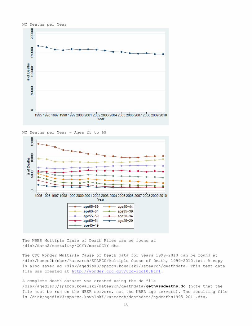
Mortality Data We use the Center for Disease Control and Prevention/National Center for Health Statistics Multiple Cause of Death data. The detailed public use data files, which are available on the NBER server for the years 1995-2011, do not identify deaths by state after 2004. Accordingly, we used the copies of these data made available

17

online by the CDC for the years 1999 to 2010. These online files, however, only provide death totals by age, rather than the full detailed data. This left some ambiguity regarding the way in which the CDC files arrived at death totals, and how to replicate this counting method using the NBER files. Fortunately, the years 1999-2004 are contained in both data sets. Using these years, we determined that the CDC files take the death totals directly from the variable staters, state of residence, without taking note of state of occurrence. Thus, we use this method for the years 1995-1998 as well. Using this method, we retain continuity in our method of counting deaths. The totals include deaths of New York residents that occur outside of New York, and do not include deaths of non-residents that occur inside the state.

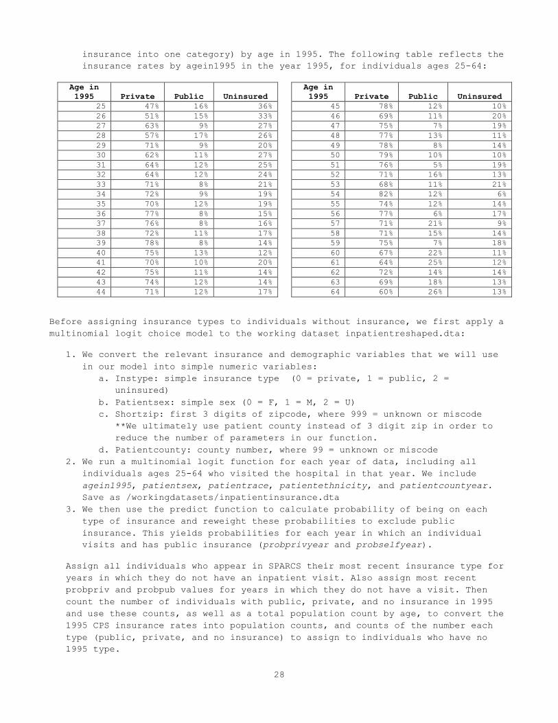
The following graphs show the deaths of NY residents in each year, first, in total, and second, by age (NOT age cohort). As these graphs show, there is no discontinuity between the years 1998 and 1999, where we change data sources.

18

NY Deaths per Year

NY Deaths per Year – Ages 25 to 69

The NBER Multiple Cause of Death Files can be found at /disk/data2/mortality/CCYY/mortCCYY.dta.

The CDC Wonder Multiple Cause of Death data for years 1999-2010 can be found at /disk/homes2b/nber/katearch/SPARCS/Multiple Cause of Death, 1999-2010.txt. A copy is also saved ad /disk/agedisk3/sparcs.kowalski/katearch/deathdata. This text data file was created at http://wonder.cdc.gov/ucd-icd10.html.

A complete death dataset was created using the do file /disk/agedisk3/sparcs.kowalski/katearch/deathdata/getnvssdeaths.do (note that the file must be run on the NBER servers, not the NBER age servers). The resulting file is /disk/agedisk3/sparcs.kowalski/katearch/deathdata/nydeaths1995_2011.dta.

19

Unfortunately, mortality data for NY state with 1 year age categories is not available for the year 2011 from the CDC at this time. Currently we use the 2010 data again for 2011. 2011 data should become available in fall 2013, per discussion with CDC Wonder staff (spoke with Sigrid cwus@cdc.gov 888-496-8347 on 8/8/13).

Population Data We use the US Census intercensal population estimate data file for 1995 to construct our NY population cohort. These data identify the NY population for each year of age from 0 to 84 (ages 85 and older are consolidated into a single category). The 1995 population estimates are contained within the file /disk/oldadmin/homes/web/html/data/census-intercensal-population/pop90s.dta on the NBER public server.

A complete population dataset for the years 1995 – 2010 is available for reference. It was created using /disk/agedisk3/sparcs.kowalski/katearch/popdata/getpopulation.do and is saved as /popdata/nypopulation1995_2010.

Part I: Within-Sample Balancing

First, we create an observation for every individual age 25-64 (in 1995) who ever appears in SPARCS in every year of our sample period. In years where an individual did not visit the hospital, we simply create an observation where all fields are missing, except for agein1995 and deathyear. At this stage, the dataset contains an annual observation for each ENC_ENHANCED_UPID that ever appears in the SPARCS inpatient data. If an individual dies, they remain in the dataset, but their deathyear indicates that they are dead (and as they do not visit the hospital in years following their year of death, those fields are coded as “missing” in later years).

Part II: State Population Balancing

Balancing the Dataset to Match NY State Population & Death Totals We complete the process of balancing the working dataset to match the 1995 NY state totals in two steps. Again, we include only individuals who are ages 25-64 in 1995 in the balanced sample.

1. First, we build observations to match the mortality totals in NY state for the years 1995-2011. That is, we add observations for individuals who die during our sample period according to the mortality records, and are not recorded as dying in SPARCS. We allocate ages and death years to these individuals such that the combination of these individuals plus the dying individuals observed in SPARCS match the age and year of death distribution observed in the state mortality totals.

a. We count the number of deaths of individuals who appear in SPARCS between 1995 and 2011, and group these dying people by “age in 1995” and year of death.

b. We also calculate the total deaths by “age in 1995” and year of death in the state of New York for the years 1995-2010. We use the 2010 data again to simulate deaths in 2011 by “age in 1995”.

c. We then find the difference between the NY population and SPARCS population totals for each age-deathyear category. These differences are equal to the number of people in each age-deathyear cohort of the 1995 NY population who die between 1995 and 2011, but do not visit the

20

hospital. We create an observation for each individual in this set. We give each individual a unique id, reshape to create an observation for each individual in each year, and apply the year of death to each observation, by unique id. The result is a dataset of the following form:

id year deathyear agein1995 deadny+_n 1995-2011 1995-2011 25-64 yrs

We can then append this dataset to the SPARCS balanced dataset. Together, the SPARCS and non-SPARCS deaths account for all of the 895,425 total deaths in NY from 1995-2011 among individuals who were age 25-64 in 1995:

Death Year

Deaths in SPARCS Population Non-SPARCS

Deaths Total Deaths

Death in Hospital

Death from NVS Data

Total SPARCS Deaths

1995 14,146 5,496 19,642 22,936 42,578 1996 14,552 9,044 23,596 17,804 41,400 1997 14,788 10,595 25,383 14,142 39,525 1998 15,803 11,972 27,775 12,541 40,316 1999 17,102 13,564 30,666 12,299 42,965 2000 18,652 14,655 33,307 11,725 45,032 2001 19,376 16,431 35,807 12,717 48,524 2002 20,833 17,820 38,653 11,280 49,933 2003 22,031 18,812 40,843 10,640 51,483 2004 22,319 19,643 41,962 11,218 53,180 2005 22,935 21,980 44,915 10,611 55,526 2006 23,556 23,169 46,725 10,515 57,240 2007 24,404 25,019 49,423 10,352 59,775 2008 26,027 26,542 52,569 10,257 62,826 2009 26,612 28,620 55,232 10,360 65,592 2010 27,133 19,963 47,096 20,956 68,052 2011 28,415 28,584 56,999 14,479 71,478 Total 358,684 311,909 670,593 224,832 895,425 *While 2,111,793 deaths were observed in SPARCS, only 670,593 individuals aged 25-64 in 1995 died by 2011.

Deaths in the SPARCS population comprise 75% of the Deaths observed in New York from 1995 to 2011 in this cohort. 40% of all deaths are deaths observed in the hospital and indicated by the SPARCS dataset, and 35% are deaths provided by the New York Department of Vital Statistics.

2. After accounting for the “SPARCS population” and the “Non-SPARCS population

that dies at some time during the sample period”, we can then derive the remaining NY population for each age group, recalling that we seek to maintain the 1995 NY population age distribution in each year of the sample.

a. We count the number of individuals in each age group contained in the appended dataset created at the end of step 1 (this gives us total SPARCS population + Non-SPARCS dying population). We then subtract these population totals by age group from the 1995 NY population. This yields the remaining NY population by age that must be added to the dataset in order to account for the total 1995 population of NY in each year.

b. We expand these totals, to create an observation for each individual in this set. As before, we give each individual a unique id and reshape to

21

create an observation for each individual in each year. This yields a dataset of the following form:

id year deathyear agein1995 aliveny+_n 1995-2011 . 25-64 yrs

As we discuss more thoroughly in the section “sources of error”, the total population of the dataset exceeds the total 1995 population of New York by 4,154 individuals. This is because for ages 62-63, the sum of the individuals observed in SPARCS and the additional individuals who die during 1995-2011 exceeds the total population of these cohorts observed in the 1995. In order to retain observations for all of the individuals who appear in SPARCS in this age cohort, as well as the mortality total for this group, we allow these age cohorts to slightly exceed the population total for the group. This phenomenon is highlighted in blue on the table on page 22.

c. We then append this dataset to the dataset created in step 1. The graphic below illustrates the composition of the final working dataset:

We recode the individual IDs to count the number of individuals in the dataset (the ids thus range from 1 to 9,554,430). The final working dataset is composed of the SPARCS data, a set of individuals with no hospital visits but with death dates and ages, and a set of individuals with ages, but no visits and no death date. There are 17 observations of each individual, one in each year. There are a total of 9,554,430 individuals in the final set. The composition of the working dataset is detailed in the table on page 22.

We consider an individual to be dead the period following their death (ie. if the current year > death year). The following table summarizes the portion of the population that is dead in each year. It is important to keep in mind that we observe more deaths than there are dead individuals in 2011. This is because individuals who are observed to die in the year 2011 or 2012 are never observed as dead during the sample period (they would not be considered dead until 2012 or 2013):

Year # Dead

1995 1996 1997 1998 1999 2000 2001 2002 2003 2004 2005 2006 2007 2008 2009 2010 2011#  Individuals

Year

These  individuals  are  observed  in  SPARCS, and  die  between  1995  and  2011.  Maroon  indicates  that  they  are  dead  in  a  given  year.

These  individuals  are  observed  in  SPARCS  and  are  still  alive  in  2011.

These  are  New  Yorkers  not  observed  in  SPARCS,  who  die  in  the  years  1995  -­‐ 2011.  Dark  green  indicates  that  they  are  dead.

These  are  New  Yorkers  not  observed  in  SPARCS,  who  do  not  die  in  the  years  1995   -­‐ 2011.

6,030,085

670,593

224,832

2,628,920

9,554,430

22

1996 42,578 1997 83,978 1998 123,503 1999 163,819 2000 206,784 2001 251,816 2002 300,340 2003 350,273 2004 401,756 2005 454,936 2006 510,462 2007 567,702 2008 627,477 2009 690,303 2010 755,895 2011 823,947

Composition of Working Dataset

Age in

1995

Individuals in SPARCS Individuals Not in SPARCS

Total Cohort

Actual 1995 NY

Population Cohort Pop. - Actual Pop.

Death Observed in 1995-2011

No Death Observed

Death Observed in 1995-2011

No Death Observed

25 2,592 215,029 2,364 52,165 272,150 272,150 0 26 2,842 210,527 2,542 49,966 265,877 265,877 0 27 3,116 206,189 2,656 52,998 264,959 264,959 0 28 3,494 205,293 3,166 45,994 257,947 257,947 0 29 3,956 207,907 3,401 82,945 298,209 298,209 0 30 4,439 208,231 3,813 87,822 304,305 304,305 0 31 5,005 207,271 4,155 86,887 303,318 303,318 0 32 5,755 202,302 4,549 95,015 307,621 307,621 0 33 6,146 192,140 4,646 106,033 308,965 308,965 0 34 6,836 190,017 5,060 126,702 328,615 328,615 0 35 7,667 183,726 5,026 125,677 322,096 322,096 0 36 8,161 177,110 5,519 115,937 306,727 306,727 0 37 8,985 173,420 5,664 117,339 305,408 305,408 0 38 9,650 168,385 5,676 98,457 282,168 282,168 0 39 10,401 159,426 6,076 135,366 311,269 311,269 0 40 11,280 160,068 6,307 119,082 296,737 296,737 0 41 12,225 152,649 6,345 103,827 275,046 275,046 0 42 13,000 148,981 6,269 100,537 268,787 268,787 0 43 13,935 146,882 6,412 94,496 261,725 261,725 0 44 14,511 145,765 6,704 105,002 271,982 271,982 0 45 15,781 145,345 6,451 93,913 261,490 261,490 0 46 16,666 146,062 6,676 76,507 245,911 245,911 0 47 18,206 147,132 7,138 75,673 248,149 248,149 0 48 20,729 157,669 5,922 68,401 252,721 252,721 0 49 17,445 125,501 6,518 61,218 210,682 210,682 0 50 18,966 124,254 5,521 59,502 208,243 208,243 0 51 20,263 124,006 6,247 46,398 196,914 196,914 0 52 23,745 133,916 5,743 45,417 208,821 208,821 0 53 22,652 119,913 5,788 35,167 183,520 183,520 0 54 23,060 113,105 5,546 41,995 183,706 183,706 0 55 24,140 112,524 5,751 28,062 170,477 170,477 0 56 25,630 109,449 5,697 26,987 167,763 167,763 0 57 26,864 108,949 6,243 23,223 165,279 165,279 0 58 28,364 105,420 6,033 6,701 146,518 146,518 0 59 29,897 104,137 6,506 16,507 157,047 157,047 0 60 32,427 103,000 6,485 11,453 153,365 153,365 0 61 33,437 96,798 7,092 2,105 139,432 139,432 0 62 36,844 98,095 7,285 0 142,224 140,025 2,199 63 39,021 96,463 7,716 0 143,200 141,245 1,955 64 42,460 97,029 8,124 7,444 155,057 155,057 0

Total 670,593 6,030,085 224,832 2,628,920 9,554,430 9,550,276 4,154

23

Potential Sources of Error

Immigration We are obliged to assume that individuals do not enter or leave the state during the sample period. This means that we must assume that all of the individuals who appear in SPARCS were part of the New York population on July 1, 1995, and that all of the death records from the sample period reflect deaths of individuals from the 1995 population, rather than hospital visits or deaths of individuals moving into the state at a later time. This means that we likely overestimate the number of people from the 1995 New York population who visit the hospital. We also overestimate the number of people from this population who die. We believe that this is the source of the excess population in the older cohorts. Because the aging population is more likely to visit the hospital and more likely to die, any immigration into the state should be most evident in these age cohorts in the SPARCS data (since we probably see most age 60+ people in the hospital at some point, the fact that we are counting too many people is more evident). The following table shows that it is only the combined SPARCS population count that exceeds the 1995 population estimate:

Age in 1995

New York Population

SPARCS Combined

1995 to 2011 Population

SPARCS 1995 Population

NY Population Less Combined SPARCS Pop.

NY Population Less 1995 SPARCS

Population 67 147,072 147,217 20,559 (145) 126,513 68 134,939 145,530 21,319 (10,591) 113,620 69 138,719 144,507 21,267 (5,788) 117,452 70 134,996 144,385 21,674 (9,389) 113,322 71 127,952 141,785 21,809 (13,833) 106,143 72 124,516 138,054 22,074 (13,538) 102,442 73 119,139 135,276 22,279 (16,137) 96,860 74 117,666 129,995 22,343 (12,329) 95,323 75 106,822 125,278 22,059 (18,456) 84,763 76 97,672 111,878 20,528 (14,206) 77,144 77 92,749 109,932 20,941 (17,183) 71,808 78 89,542 101,369 20,050 (11,827) 69,492 79 87,625 95,349 19,847 (7,724) 67,778 80 77,302 92,743 19,799 (15,441) 57,503 81 70,857 85,256 18,953 (14,399) 51,904 82 65,148 78,152 18,100 (13,004) 47,048 83 58,165 69,302 16,844 (11,137) 41,321 84 52,899 62,227 15,940 (9,328) 36,959

It is interesting to note that the age 0 population also produces this issue, both for the aggregate SPARCS population and the 1995 population, when age is measured in December rather than in July. We believe that this is because the cohort with age measured at the end of the year includes some infants not yet born as of the population count. When age is measured in July, as it is above, the problem shifts to include age 67 and exclude age 0.

Age Calculations Our population data, SPARCS data, and mortality (death record) data all provide age in one year intervals. Thus we match the distribution of the population and distribution of deaths using 1 year age cohorts. Unfortunately, each of the data sources differs in the way that age information is derived, which introduces some error into our dataset.

24

• The population data reports the number of individuals in each age group as of 7/1 of the year in question. We calculate age in 1995 as follows:

"𝑎𝑔𝑒  𝑖𝑛  1995" = 1995 − "𝑑𝑎𝑡𝑎  𝑦𝑒𝑎𝑟" + "𝑎𝑔𝑒  𝑖𝑛  𝑑𝑎𝑡𝑎  𝑦𝑒𝑎𝑟" Thus, age in 1995 is as of 7/1/1995.

• The mortality data does not identify age as of a stable date (such as 12/31 or 7/1). Rather, it provides the age at death of individuals who died within a given calendar year. We are obliged to calculate age in 1995 as:

"𝑎𝑔𝑒  𝑖𝑛  1995" = 1995 − "𝑦𝑒𝑎𝑟  𝑜𝑓  𝑑𝑒𝑎𝑡ℎ" + "𝑎𝑔𝑒  𝑎𝑡  𝑑𝑒𝑎𝑡ℎ" Thus, age at death simply means age at some point in 1995. On average, though, we expect that half of the population dies prior to their birth month, and half dies following their birth month, making the sampling of ages at death somewhat equivalent to sampling age on 7/1. To confirm this expectation, we assessed the relationship between death months and birth months in the SPARCS sample and found that this does appear to be the case: Variable | Obs Mean Std. Dev. -------------------+----------------------------------- Death after Birth | 2111793 .4525803 .4977464 Death before Birth | 2111793 .458652 .4982875 Same month | 2111793 .0887677 .2844082

• SPARCS data provides patient date of birth, to varying degrees of accuracy. When month of birth is not provided, we assume a birth month of January. We calculate age in 1995 as of 6/30.

Though the three different approaches to calculating age should all approximate populations at the midpoint of the year, they leave room for some minor discrepancies. When SPARCS age is calculated in December, we see more deaths in SPARCS than in the NY population for some agein1995-year of death combinations, particular at very old or very young ages. The table below shows the extent of these discrepancies. The y axis is agein1995, and the x axis is the difference between total NY deaths and SPARCS deaths for each death-year. As these discrepancies disappear when we calculate age in July rather than December, we attribute them to differences between the age calculations in SPARCS and age calculations in the mortality data.

25

Timing of Cohort Measurement Ideally, we hope to follow a single cohort of people – the residents of NY in 1995. Unfortunately, while our population data reflects the population of NY as of a specific date in 1995, our mortality data and SPARCS data include people who were residents of the state at the time of a given event (a hospital visit or death). Thus, while hospital visits and deaths are being measured for everyone who appears in 1995, the population is counted only on July 1. Our population cohort is the population on one day, but the SPARCS and mortality cohorts are not measured on one day, they are the combination of measurements throughout the year. There is no clean way to adjust for this issue, but it is important to keep in mind as a source of error. Institutionalized Population Because the “SPARCS plus dying” population exceeds the 1995 population count only for ages 61 and above, we considered the possibility that the intercensal population estimate was underestimating older populations. This seemed particularly likely because the mortality data is based on death certificate records, a very precise source of data, while the intercensal estimates are based on census surveys. If the survey excluded or undercounted institutionalized populations (such as people in nursing homes), it would disproportionately underestimate the older population. We therefore reviewed the 2000 census methodology. According to the 2000 census residence rules, “People in nursing or convalescent homes for the aged or dependent [are] counted at the nursing or convalescent home” (http://www.census.gov/population/www/censusdata/resid_rules.html). While it is

Age in 1995 1995 1996 1997 1998 1999 2000 2001 2002 2003 2004 2005 2006 2007 2008 2009 2010

-15 33

-14 458 (25)

-13 482 (16) 9

-12 490 (8) 14 2

-11 497 (15) 21 24 11

-10 515 (17) 21 25 13 5

-9 502 (2) 35 23 17 4 19

-8 482 (11) 31 15 8 10 15 7

-7 515 (4) 6 21 19 17 14 2 19

-6 565 5 25 21 8 5 11 6 15 6

-5 601 - 24 15 14 10 10 7 20 14 11

-4 693 (2) 26 19 14 16 15 8 5 - 13 19

-3 634 (20) 27 11 9 6 12 18 16 14 12 15 17

-2 675 (12) 17 4 18 7 9 6 - 5 10 6 12 10

-1 742 - 26 41 15 16 20 21 20 10 13 14 17 16 16

0 777 (20) 17 34 13 26 14 9 2 20 10 6 13 12 17 32

81 1,601 1,069 928 765 805 635 467 362 362 326 227 179 71 (38) 36 581

82 1,614 1,235 971 893 786 663 481 561 315 376 232 230 247 90 (26) 542

83 1,514 1,282 958 677 575 389 444 232 187 140 97 23 (40) (28) (1) 377

84 1,758 1,190 1,124 975 766 652 418 477 317 256 164 112 1 (15) (36) 299

85 1,515 1,106 848 668 582 330 315 324 194 203 74 23 45 (18) (35) 1,393

86 1,653 1,063 837 797 583 604 436 187 127 195 61 20 (22) 18 1,040

87 1,450 1,080 989 664 605 356 235 293 161 6 44 33 4 1,006

88 1,375 1,030 791 522 432 348 178 144 67 120 (45) (61) 989

89 1,398 912 703 602 379 254 237 61 75 40 78 1,063

90 1,223 864 585 504 393 206 191 170 75 46 987

91 1,044 858 639 498 293 262 101 14 71 984

92 1,177 757 623 400 280 149 75 100 1,008

93 808 571 373 222 188 25 79 1,039

94 920 643 425 303 189 147 1,101

95 671 390 248 195 48 980

96 605 371 235 162 1,071

97 469 274 213 1,094

98 431 273 1,059

99 317 1,129

100 670

26

still possible that correctly counting this population is more difficult, it appears that the Census makes every effort to account for this population.

VI. Completing the Working Dataset

The final step in completing the working dataset is to reshape the data to “wide” form, so that there is a single observation for every individual in the dataset.

Procedure

The reshape retains a minimal number of variables – deathyear, cost, agein1995, id. It also makes a few minor changes to the data so that it is compatible with the reclassification modeling code. In particular, a set of “alreadydeadCCYY” variables are created, and all observations where costs are missing are changed to costs==0. The reshaped data is the master “working dataset,” which can be used with the reclassification modeling code. All working datasets, beginning with this master set, are saved in the workingdatasets directory. The reshape code also creates smaller working datasets, comprised of a subsection of observations. The working datasets created by inpatientreshape.do are all saved at /katearch/workdingdatsets/ and are as follows:

File Name Description inpatientreshaped.dta This is the master working dataset, containing all

observations in the balanced data.

VII. Insurance Type Assumptions

Because we only know insurance type for individuals when they appear in the hospital, we must make an assumption about these individuals during years when they are not in the SPARCS data. For the individuals who never appear in SPARCS, we will need to make an assumption in every year. We assign insurance type (as described in the variable paymentsource) as follows:

If an individual appears in SPARCS, we assign them the payment type of their most recent SPARCS visit. Thus for individuals who appear in SPARCS at least once, insurance type is decided in this manner for all years following their first visit.

For individuals who do not visit in 1995, an insurance type must be assigned until they first appear in SPARCS. We use the CPS march supplement to calculate the percentage of the population by age with public, private, and no insurance in 1995. We then randomly assign one of these three insurance types in 1995 by age according to these CPS insurance distributions. Individuals retain their 1995 insurance type until they appear in SPARCS.

Before assigning insurance types to individuals without insurance, we use the existing insurance information within SPARCS to determine the insurance choices (private vs uninsured) that the publicly insured individuals would make, absent the safety next. We determine the probability that each individual would choose private insurance and the probability that they would go uninsured, based on their characteristics and the characteristics of individuals with private and no insurance by using a multinomial logit function. We do this before applying insurance type to individuals with a missing type so that our function bases

27

predictions only on the accurate demographics/insurance type combinations observed in SPARCS.

Insurance Type

The variable “Source of Payment Code” provides insight into the type of insurance (or lack thereof) used by individuals who visit the hospital. The possible payment codes are as follows:

"A"=Self-Pay "B"=Workers' Compensation "C"=Medicare "D"=Medicaid "E"=Other Federal Program "F"=Insurance Company "G"=Blue Cross "H"=CHAMPUS "I"=Other Non-Federal Program We further simplify these categories into four major groups:

Group Name Payment Codes Included Private Insurance (“Private”) F G Government-Provided Insurance (“Public”) C D E H I Self-Pay (“Self”) A Other Payer (“Other”) B L

We then graph the frequency of these groups, out all individuals in the reference group who visit the hospital in a given year.

Procedure

Use the 1995 CPS March supplement from the NBER files to determine coverage rates:

1. We use the CPS March supplements available from the NBER. Directions to access these files are available at http://www.nber.org/data/current-population-survey-data.html. The current NBER location of these files is /disk/nber10/SCCS/cps/cpsmarchYYYY. We determine insurance type in the CPS files according to the rules recommended by the Census (www.census.gov/hhes/www/hlthins/methodology/programming/cps/recoding.html). This is not a mutually exclusive set of categories, so we then apply the Kaiser Family Foundation’s recommend coverage type hierarchy (http://kff.org/other/state-indicator/total-population/):

Hierarchy Medicaid Medicare CHAMPUS Private Uninsured (Self Pay)

2. Within the file assigninsurance.do, we then generate weighted insurance rates

for private, public, and no insurance (for now, we group all types of public

28

insurance into one category) by age in 1995. The following table reflects the insurance rates by agein1995 in the year 1995, for individuals ages 25-64:

Age in 1995 Private Public Uninsured

25 47% 16% 36% 26 51% 15% 33% 27 63% 9% 27% 28 57% 17% 26% 29 71% 9% 20% 30 62% 11% 27% 31 64% 12% 25% 32 64% 12% 24% 33 71% 8% 21% 34 72% 9% 19% 35 70% 12% 19% 36 77% 8% 15% 37 76% 8% 16% 38 72% 11% 17% 39 78% 8% 14% 40 75% 13% 12% 41 70% 10% 20% 42 75% 11% 14% 43 74% 12% 14% 44 71% 12% 17%

Age in 1995 Private Public Uninsured

45 78% 12% 10% 46 69% 11% 20% 47 75% 7% 19% 48 77% 13% 11% 49 78% 8% 14% 50 79% 10% 10% 51 76% 5% 19% 52 71% 16% 13% 53 68% 11% 21% 54 82% 12% 6% 55 74% 12% 14% 56 77% 6% 17% 57 71% 21% 9% 58 71% 15% 14% 59 75% 7% 18% 60 67% 22% 11% 61 64% 25% 12% 62 72% 14% 14% 63 69% 18% 13% 64 60% 26% 13%

Before assigning insurance types to individuals without insurance, we first apply a multinomial logit choice model to the working dataset inpatientreshaped.dta:

1. We convert the relevant insurance and demographic variables that we will use in our model into simple numeric variables:

a. Instype: simple insurance type (0 = private, 1 = public, 2 = uninsured)

b. Patientsex: simple sex (0 = F, 1 = M, 2 = U) c. Shortzip: first 3 digits of zipcode, where 999 = unknown or miscode

**We ultimately use patient county instead of 3 digit zip in order to reduce the number of parameters in our function.

d. Patientcounty: county number, where 99 = unknown or miscode 2. We run a multinomial logit function for each year of data, including all

individuals ages 25-64 who visited the hospital in that year. We include agein1995, patientsex, patientrace, patientethnicity, and patientcountyear. Save as /workingdatasets/inpatientinsurance.dta

3. We then use the predict function to calculate probability of being on each type of insurance and reweight these probabilities to exclude public insurance. This yields probabilities for each year in which an individual visits and has public insurance (probprivyear and probselfyear).

Assign all individuals who appear in SPARCS their most recent insurance type for years in which they do not have an inpatient visit. Also assign most recent probpriv and probpub values for years in which they do not have a visit. Then count the number of individuals with public, private, and no insurance in 1995 and use these counts, as well as a total population count by age, to convert the 1995 CPS insurance rates into population counts, and counts of the number each type (public, private, and no insurance) to assign to individuals who have no 1995 type.

29

1. Continue using /workingdatasets/inpatientreshaped.dta and assign most recent insurance type to all years where an individual does not appear in SPARCS (this will be missing until an individual appears in SPARCS for the first time). Then collapse the by agein1995 to create a dataset of the number of individuals in each age year with public, private, and no insurance, as well as the total number of individuals of each age in the dataset. Save as /workingdatasets/popdata.dta.

2. Merge popdata.dta on to the CPS insurance rate file (/cpsdata/CPS1995_2011.dta) by age in 1995. Multiply total population by the cps public, private, and no insurance rates to come up with a count of the number of people in 1995 of each age who should have public, private, and no insurance.

a. Rounding these counts up or down to the nearest person will mean that in some cases the sum of the private, public, and no insurance counts will differ from the total population count by +/- 1. To ensure that the sum of the three categories is equal to the total population, add one individual to the category that was closest to being rounded up instead of rounded down, or subtract one from the category that was closest to being rounded down, as necessary. Save as /workingdatasets/inpatientcomplete.dta. Ex:

Exactly Calculated Population (CPS Rate * Total Pop) Rounded Population

Public Private Self Total Public Private Self Total 4.55 3.9 1.55 10 5 4 2 11

REVISION: Round down decimal greater than .5 but closest to .5 Public Private Self Total Public Private Self Total

4.00 3.9 1.56 10 4 4 2 10