Space in Unified Models of Economy and Ecology

or . . . ? Space: The final frontier

A. Xepapadeas*University of Crete, Department of Economics

*Research presented in this lecture has been conducted jointly with William Brock.

• Economics studies how human societies use scarce resources to produce commodities and distribute them among their members.

• Ecology is the study of living species, such as animals, plants and micro-organisms and the relations among themselves and their natural environment. An ecosystem includes these species and their nonliving environment, their interactions and evolution in time and space.

• Human economies and natural ecosystems are inexorably linked, but economic models and ecological models are not usually linked. Ecological economics aims at providing this link.

Economic and ecological systems evolve in time and space. Interactions take place among units occupying distinct spatial points. Thus geographical patterns of production activities, urban concentrations, or species concentrations occur. My purpose is:

• to discuss approaches for modeling, in a meaningful way, economic and ecological processes evolving in space time.

• to examine mechanism under which a spatially homogenous state – a flat landscape – acquires a spatial pattern.

• to examine how this pattern evolves in space-time.

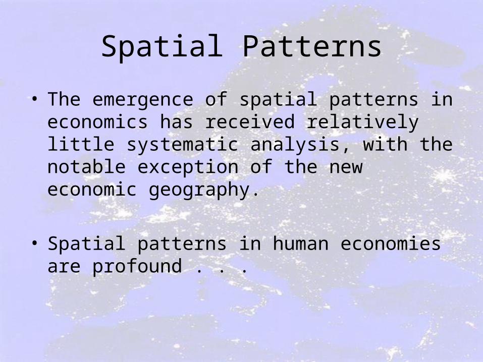
• The emergence of spatial patterns in economics has received relatively little systematic analysis, with the notable exception of the new economic geography.

• Spatial patterns in human economies are profound . . .

Spatial Patterns

Spatial Analysis in Economics

• However spatial analysis was not given sufficient attention until the early 1990s

• Main ideas in location theory rely on economies of scale that enforce geographical concentrations

• Inability of earlier research to work with tractable models of imperfect competition which is implied by unexhausted economies of scale.

• In a homogeneous environment with transportation costs but no returns to scale, spatial patterns of economic activity cannot emerge. Economic activity should spread evenly across space to minimize transportation costs.

• Need for increasing returns to generate spatial patterns

• Need to model imperfect competition• Increasing returns/Imperfect competition

– New Industrial Organization– New Trade Theory – New Growth Theory – New Economic Geography

The Racetrack Economy*• Many regions equally spaced around the

circumference of a circle• Transportation takes place around the

circumferences• From a spatially homogeneous – flat – initial

distribution of manufacturing activities, a perturbation generates a spatial structure. Manufacturing is concentrated in two regions.

• What is the mechanism that generates this spatial pattern?

*M. Fujita, P. Krugman and A. Venables, The Spatial Economy, MIT Press 2001.

Paul Krugman, “Space: The Final Frontier” Journal of Economic Perspectives, Vol. 12, 2, 1998, pp. 161-174

Spatial Analysis in Ecology• Pattern formation and the emergence of

spatial patterns have received relatively more attention in ecology.

• Morphogenesis is the study of patterns and form, e.g.:– Mammalian coat patterns– Butterfly wing patterns

• Spatial patterns in resources.• Spatial patterns of species.• The concept of diffusion has been used in

ecological modeling to explain spatial pattern formation in ecological systems.

How the leopard got its spots

Spatial patterns in Kilimanjaro

Chlorophyll concentrations in oceans

Locust distribution in Australia

Modelling Diffusion• Biological resources tend to disperse in space

and time under forces promoting "spreading" or "concentrating" (Okubo, 2001); these processes along with intra and inter species interactions induce the formation of spatial patterns.

• Economic activities also tend to disperse in space and time. Flows of capital, labour, commodities, resources

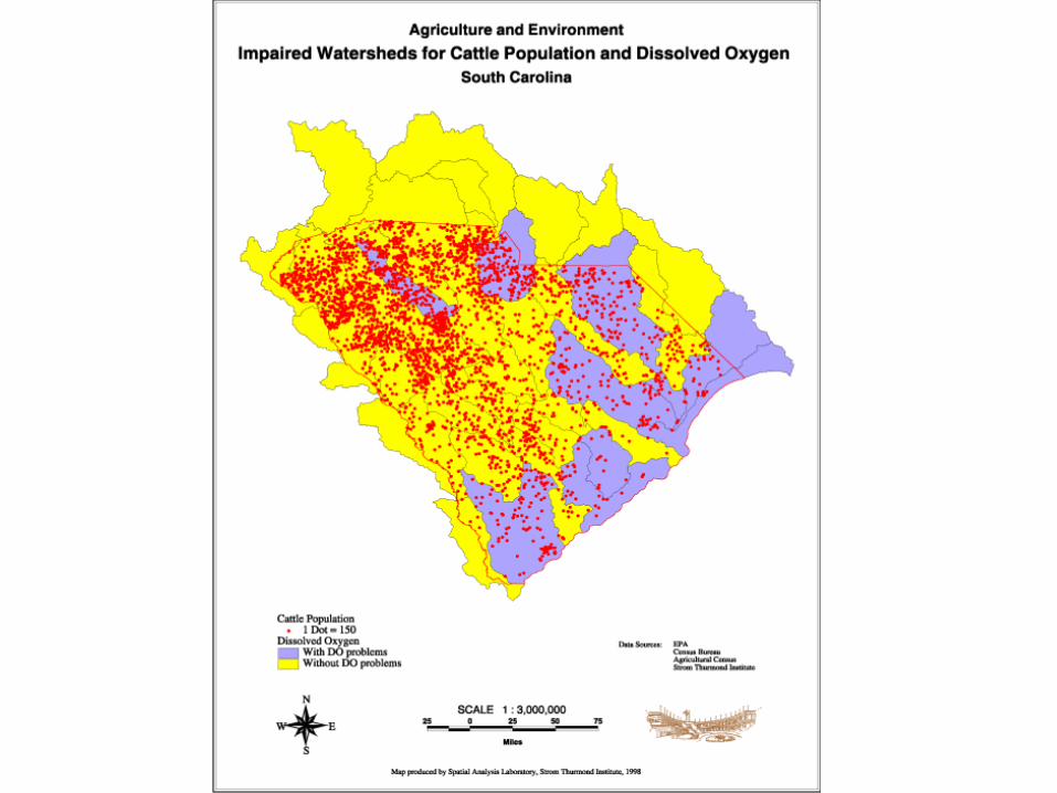
• Spatial issues in economic-ecological problems: – resource management in patchy environments

(Sanchirico and Wilen 1999, 2001; Sanchirico 2004; Brock and Xepapadeas 2002)

– the study of control models for interacting species (Lenhart and Bhat 1992, Lenhart et al. 1999)

– the control of surface contamination in water bodies (Bhat et al. 1999)

• A central concept in modelling the dispersal of biological or economic resources is that of diffusion.

• Diffusion is defined as a process where the microscopic irregular movement of particles such as cells, bacteria, chemicals, animals, or commodities, results in some macroscopic regular motion of the group (Okubo and Levin 2001; Murray 1993, 2003).

• Diffusion is based on random walk models, which when coupled with population growth equations or capital accumulation equations lead to general reaction-diffusion systems.

Let tzx , denote the concentration of a biological or economic

variable at time t 0 at the spatial point .z Space is assume to be a line. We assume that the flux of ‘material’ animals, commodities, is proportional to the gradient of the concentration of the material , or

z

tzxDtz x

,,

where xD is the diffusion coefficient and the minus sign indicates that material moves from high levels of concentration to low levels or concentration Under this diffusion assumption the evolution of the material’s stock in a small interval z is defined as

dstsFtzztzdstsxdt

d zz

x

zz

z,,,,

(1)

where txF , is a growth function for the material in question Dividing (1) by z and taking limits as ,0z the evolution of the material is determined as:

tzFx

tz

t

tzx,

,,

Using the definition of diffusion we obtain the basic diffusion equation

2

2 ,,

,

x

tzxDtzF

t

tzxx

• In general a diffusion process in an ecosystem tends to produce a uniform population density, that is spatial homogeneity. Thus it might be expected that diffusion would "stabilize" ecosystems where species disperse and humans intervene through harvesting.

• There is however one exception known as diffusion induced instability, or diffusive instability (Okubo et al. 2001). Alan Turing (1952) suggested that under certain conditions reaction-diffusion systems can generate spatially heterogeneous patterns. This is the so-called Turing mechanism for generating diffusion instability.

Emergence of Spatial Patterns

• We examine conditions under which the Turing mechanism induces diffusive driven instability and creates heterogeneous spatial patterns in Economic/Ecological models.

• This is a different approach to the one most commonly used to address spatial issues, which is the use of metapopulation models in discrete patchy environments with dispersal among patches.

• Thus the Turing mechanism can be used to uncover conditions which generate spatial heterogeneity in models where ecological variables interact with economic variables. When spatial heterogeneity emerges, the concentration of variables of interest (e.g. resource stock and level of harvesting effort), in a steady state, are different in different locations of a given spatial domain. Once the mechanism is uncovered, the impact of regulation in promoting or eliminating spatial heterogeneity can also be analyzed.

A Bioeconomic ModelThe movement of biomass and effort in time and space can be described by the following reaction diffusion system

2

22

2

2

,

,0for 0 given,0,),0,(

0,

z

x

z

xx

zExzEzx

EDEACpqxEt

E

xDqExrxsxt

x

E

x

where EAC is the average cost curve, assumed to be U-shaped. By (zero flux) it is assumed that there is no external biomass or effort input on the boundary of the spatial domain.

The spatially homogeneous system for biomass evolution is:

0,

EACpqxEE

qExrxsxx

where a steady state 0, Ex for the spatial homogeneous system

is determined as the solution of .0Ex Linearizing around a steady state ,, Ex the linearized spatial homogeneous system can be written as

EE

xxJ www ,

where the linearization matrix J around a steady state is defined as

2221

1211

aa

aa

EACEpqE

qxrxJ

The Turing Mechanism

• The Turing mechanism implies that the spatially homogeneous steady state can be destabilized by a spatial perturbation depending on

• Condition for diffusive instability

xE DD /

02 2/12/1211222112211 xExE DDaaaaDaDa

Linearizing the full system and we obtain

E

xt

t

D

DD

tE

tx

DJ

0

0,

/

/

,2

w

www

The solution for the biomass and effort takes the form

a

zt

aEtzE

a

zt

axtzx

E

x

cosexp,

cosexp,

2

2

2

2

Since ,02

2 a as t increases the deviation from the spatial

homogeneous solution does not die out and could eventually be transformed into a spatial pattern which is like a single cosine mode. Then the growing solution approaches, as ,t a cosine like spatial pattern, which implies spatial heterogeneity of the steady state. Figure 1, draws on Murray (2003 Vol II, pp. 94-95) to represent one possible spatial pattern for ., tzx Shaded areas represent spatial biomass

concentration above ,x while non shaded areas represent spatial biomass

Spatial Pattern

0 α/2 α z

x>x*

x<x*

Figure 1

0

5

10

15 0

10

20

30

40

50

00.51

1.52

0

5

10

15

t

z

x

λ=0.5

t

z

x

λ=-0.5

0

5

10

15 0

10

20

30

40

50

0.9

0.95

1

1.05

1.1

0

5

10

15

Capital Accumulation and Pollution Accumulation*

* Based on current research of S. Levin and A. Xepapadeas

We assume that pollution and capital diffuse along a segment 0,L. Pollution accumulation evolves in time and space according to:

Px,tt

gx,Kx,t xPx,t DP2Px,tx2

#

Capital stock evolves in time and space and according to:

Kx,tt

sxAKx,tfKx,t x,Px,tKx,t

DK2Kx,tx2

#

If the determinant of the linearization matrix around the equilibrium point

J sa AKa1 P PK

gK

does not vanish then an equilibrium exists for the spatially homogeneous system

If 1 then the a11 element of the linearization matrix is positive. In this case if

sa AKa1 P trJ 0

|J| 0 the linearization matrix has two real negative eigenvalues and the equilibrium is stable.

• The spatially homogeneous capital-pollution steady state can be destabilized by diffusive or Turing instability if:

• In this case we have a spatially heterogeneous pattern of capital accumulation (economic activity) and pollution accumulation

• But we require α11>1, increasing returns

02 2/12/1211222112211 KPKP DDaaaaDaDa

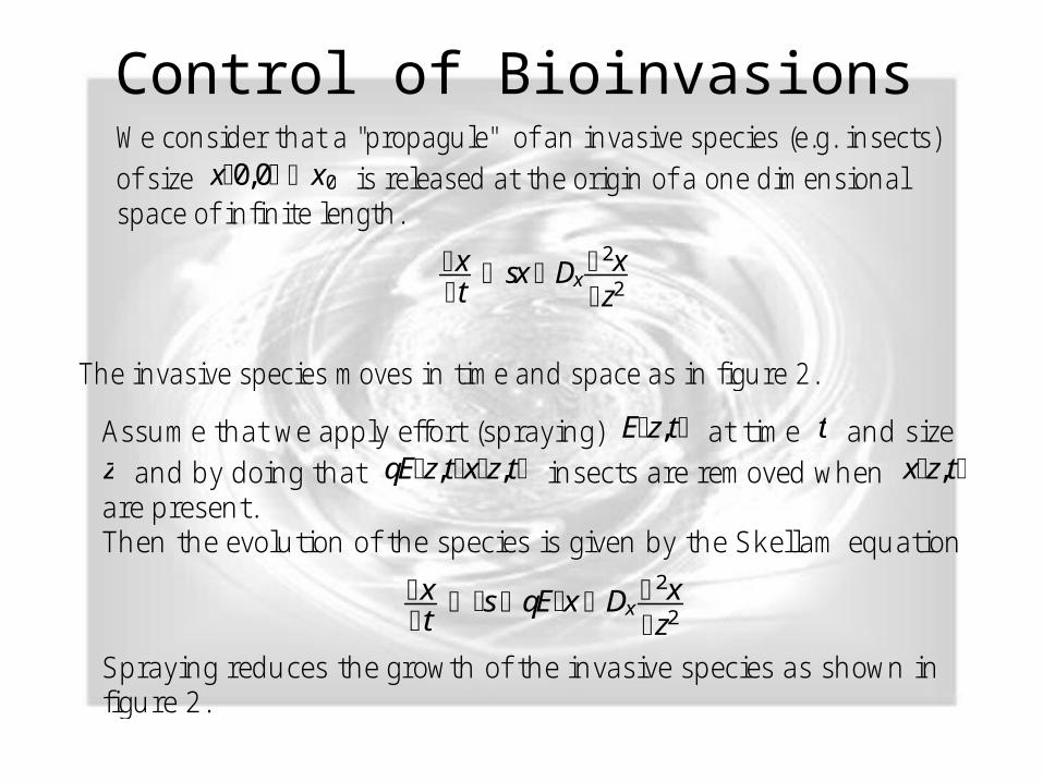
Control of BioinvasionsWe consider that a "propagule" of an invasive species (e.g. insects) of size x0,0 x0 is released at the origin of a one dimensional space of infinite length.

xt

sx Dx 2xz2

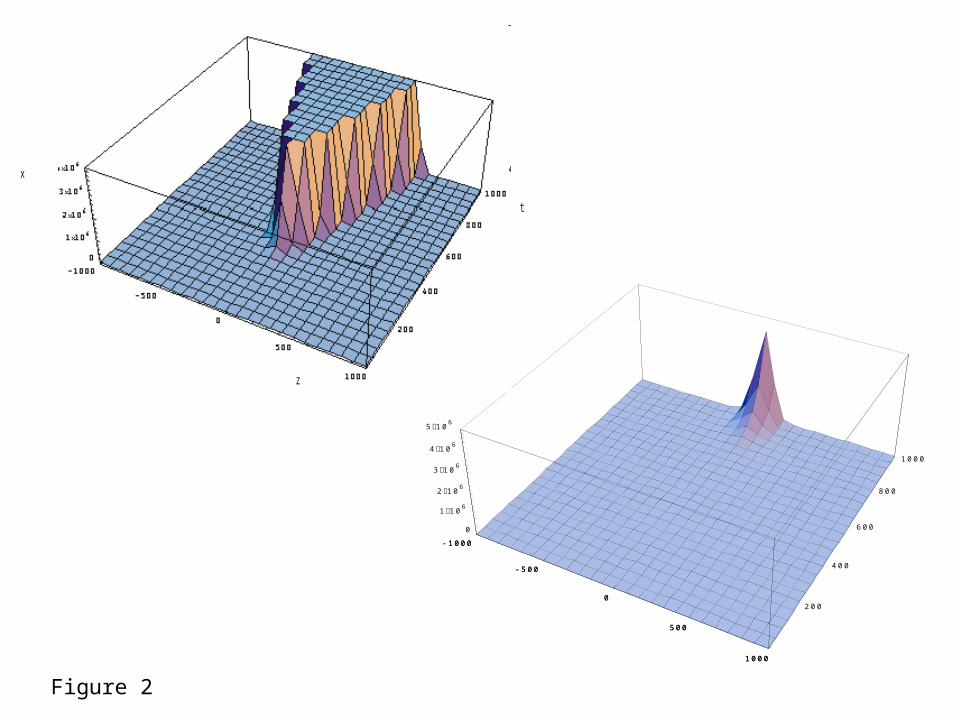
The invasive species moves in time and space as in figure 2.

Assume that we apply effort (spraying) Ez,t at time t and size z and by doing that qEz,txz,t insects are removed when xz,t are present. Then the evolution of the species is given by the Skellam equation

xt

s qEx Dx 2xz2

#

Spraying reduces the growth of the invasive species as shown in figure 2.

-1000

-500

0

500

1000

200

400

600

800

1000

0

1106

2106

3106

4106

5106

-1000

-500

0

500

1000

t

z

x

Figure 2

To make the model more realistic assume that the removal of the insects generates benefit equal to pzqEz,txz,t, where pz is the value associated with insect removal. Spraying has a time invariant average cost

ACE c0z 12c1zEz,t #

Assume that spraying moves fast across sites so that costs and benefits are equated and the p, c0 and c1 are spatially homogeneous. In this case the evolution of the invasive species is given by the Fisher equation

xt

ŝx1 âx Dx 2xz2

ŝ s 2qc0c1

, r 2q2pc1

, â rŝ

#

It can be seen that a wave solution exists for the evolution of the invasive species with minimum wave speed ,

cmin 2 s 2qc0

c1Dx

1/2

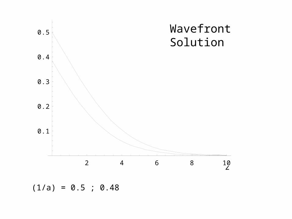
In the wave front solution the maximum concentration of the invasive species is

1â c1s 2qc0

2q2p #

Thus maximum concentration is declining in p the value associated with the removal of the invasive species.

0

5

10

15 0

10

20

30

40

50

0

10

20

30

40

0

5

10

15

Wavefront

Solution

t

z

z2 4 6 8 10

0.1

0.2

0.3

0.4

0.5 Wavefront Solution

(1/a) = 0.5 ; 0.48

Conclusions• This paper develops methods of analyzing

spatial dynamical ecological/economic systems.

• In particular the Turing mechanism for diffusive instability is adopted to bioeconomic problems

• The potential power of the method is shown in the analysis of spatial pattern formation in– A resource management problem– A spatial growth under pollution

accumulation problem– A bioinvasion control problem

Regulation Issues• In the resource management

problem and the growth pollution problem, spatial pattern creation is possible.– Spatial pattern creation may have

welfare implications regarding the spatial distribution of welfare.

– Regulation can eliminate spatial patterns and induce spatial homogeneity.

• Control of Bioinvasions– When benefits and costs are equated

across sites, the invasion could take the form of a travelling wave.

– Regulation affects the wave's speed and the spatially homogeneous stable carrying-capacity biomass of the invasive species.

We are living in a spatially heterogeneous world.. The modeling approach presented here might help in gaining some new insights into the interrelations between ecological systems and human economies and might provide a basis for more efficient regulation of environmental externalities in the space – time continuum