Space Bounded Scatter Machines

João Alves Alírio

Dissertation to obtain the Master of Science Degree in

Mathematics and Applications

Supervisor: Prof. José Félix Gomes da Costa

Examination Committee

Chairperson: Prof. Maria Cristina Sales Viana Serôdio SernadasSupervisor: Prof. José Félix Gomes da Costa

Members of the Committee: Prof. André Nuno Carvalho Soutoand Prof. João Filipe Quintas dos Santos Rasga

May 2017

Acknowledgments

I would like to thank my supervisor, Professor Jose Felix Costa, for introducing me to the subject ofComplexity Theory, for all his help and guidance in the elaboration of this work, for his availability andall the hours spent explaining and clarifying several issues, but mostly for all his patience and tolerancethrough the whole time of the work.

I would also like to thank my family for all the support and help, and my friends who accompaniedme through the work and helped and supported me.

Thank you all.

i

Abstract

This dissertation concerns the computational power of an abstract computation model when boundedin polynomial space. The computation model in study consists of a Turing machine coupled with aphysical experiment as oracle (the scatter experiment). This computation model (the scatter machine)is already studied concerning polynomial time restrictions, from where we adapted most of the prooftechniques used to this work.

We understood for which functions we are able to build a clock (a specific Turing machine) in poly-nomial space. There are clocks in polynomial space for functions with at most an exponential growingrate. We also presented a new communication protocol (the generalized protocol) between the ana-logue and the digital components of the scatter machine which, in this case, allow us to use the propercomputational power of the scatter experiment as an oracle.

We introduce a uniform complexity class, which we use as support class for one non-uniform com-plexity class needed to describe the computational results we obtained. We established the computa-tional results of the scatter machine bounded in polynomial space, for both the sharp wedge and thesmooth wedge cases, using in each case both the standard and the generalized communication proto-cols. We established the results for the three usual precision assumptions (infinite precision, arbitraryprecision and fixed precision), and in some cases of the smooth wedge experiment we obtain differentresults depending on if we use the time schedule (clock to bound the time running of the experiment) ornot.

Keywords: Analogue-digital computation; Physical oracle; Non-uniform complexity; Spacebounded clocks; Hypercomputation.

ii

Resumo

Neste trabalho estudamos o poder computacional de um modelo de computacao abstracto quandolimitado em espaco polinomial. O modelo de computacao em estudo consiste numa maquina de Tur-ing acoplada a uma experiencia fısica como oraculo (a experiencia de dispersao). Este modelo decomputacao (a maquina de dispersao) ja esta estudado em relacao a restricoes em tempo polinomial,de onde adaptamos a maioria das tecnicas de prova usadas neste trabalho.

Averiguamos quais seriam as funcoes para as quais podemos construir um relogio (uma maquinade Turing especıfica) em espaco polinomial. Existem relogios em espaco polinomial para funcoes comum crescimento no maximo exponencial. Apresentamos tambem um novo protocolo de comunicacao (oprotocolo generalizado) entre os componentes analogico e digital da maquina de dispersao que, nestecaso, permite usar todo o poder computacional da experiencia de dispersao como oraculo.

Introduzimos uma classe de complexidade uniforme, que usamos como classe de suporte parauma classe de complexidade nao uniforme necessaria para descrever os resultados computacionaisobtidos. Estabelecemos os resultados computacionais da maquina de dispersao limitada em espacopolinomial para ambas, a parede com vertice e para a parede diferenciavel, utilizando em cada caso,ambos os protocolos de comunicacao padrao e generalizado. Estabelecemos os resultados para ostres casos de precisao usuais (precisao infinita, precisao ilimitada e precisao fixa), e em alguns casosda experiencia com parede diferenciavel obtivemos resultados diferentes dependendo de se usamos orelogio temporizador (relogio para limitar o tempo de execucao da experiencia) ou nao.

Palavras-chave: Computacao analogico-digital; Oraculo fısico; Complexidade nao uniforme;Relogios limitados no espaco; Hipercomputacao.

iii

Contents

Acknowledgments . . . . . . . . . . . . . . . . . . . . . . . . . . . . . . . . . . . . . . . . . . . iAbstract . . . . . . . . . . . . . . . . . . . . . . . . . . . . . . . . . . . . . . . . . . . . . . . . . iiResumo . . . . . . . . . . . . . . . . . . . . . . . . . . . . . . . . . . . . . . . . . . . . . . . . . iiiContents . . . . . . . . . . . . . . . . . . . . . . . . . . . . . . . . . . . . . . . . . . . . . . . . ivList of Figures . . . . . . . . . . . . . . . . . . . . . . . . . . . . . . . . . . . . . . . . . . . . . vList of Tables . . . . . . . . . . . . . . . . . . . . . . . . . . . . . . . . . . . . . . . . . . . . . . vi

1 Introduction 11.1 Our work . . . . . . . . . . . . . . . . . . . . . . . . . . . . . . . . . . . . . . . . . . . . . 31.2 Mathematical preliminaries . . . . . . . . . . . . . . . . . . . . . . . . . . . . . . . . . . . 5

2 Clocks and physical oracle 122.1 Clocks . . . . . . . . . . . . . . . . . . . . . . . . . . . . . . . . . . . . . . . . . . . . . . . 122.2 Scatter experiment . . . . . . . . . . . . . . . . . . . . . . . . . . . . . . . . . . . . . . . . 172.3 Protocol . . . . . . . . . . . . . . . . . . . . . . . . . . . . . . . . . . . . . . . . . . . . . . 192.4 Scatter machine . . . . . . . . . . . . . . . . . . . . . . . . . . . . . . . . . . . . . . . . . 23

3 Standard scatter machine 263.1 Vertex position . . . . . . . . . . . . . . . . . . . . . . . . . . . . . . . . . . . . . . . . . . 273.2 Find the vertex position with fixed precision . . . . . . . . . . . . . . . . . . . . . . . . . . 293.3 Sparse oracles . . . . . . . . . . . . . . . . . . . . . . . . . . . . . . . . . . . . . . . . . . 313.4 Probabilistic trees . . . . . . . . . . . . . . . . . . . . . . . . . . . . . . . . . . . . . . . . 333.5 Boundary numbers . . . . . . . . . . . . . . . . . . . . . . . . . . . . . . . . . . . . . . . . 363.6 Sharp scatter machine . . . . . . . . . . . . . . . . . . . . . . . . . . . . . . . . . . . . . . 373.7 Smooth scatter machine . . . . . . . . . . . . . . . . . . . . . . . . . . . . . . . . . . . . . 41

4 Generalized scatter machine 474.1 Sharp scatter machine . . . . . . . . . . . . . . . . . . . . . . . . . . . . . . . . . . . . . . 484.2 Smooth scatter machine . . . . . . . . . . . . . . . . . . . . . . . . . . . . . . . . . . . . . 51

5 Conclusion 55

References 59

iv

List of Figures

2.1 Clock for f(n) = 2n · 2n + 1 . . . . . . . . . . . . . . . . . . . . . . . . . . . . . . . . . . . 142.2 Clock for f(n) = 2n · 2n−(blognc+1) + 1 . . . . . . . . . . . . . . . . . . . . . . . . . . . . . 162.3 Sharp scatter experiment . . . . . . . . . . . . . . . . . . . . . . . . . . . . . . . . . . . . 172.4 Smooth scatter experiment . . . . . . . . . . . . . . . . . . . . . . . . . . . . . . . . . . . 18

v

List of Tables

3.1 Standard communication protocol ShSM . . . . . . . . . . . . . . . . . . . . . . . . . . . . 263.2 Standard communication protocol SmSM . . . . . . . . . . . . . . . . . . . . . . . . . . . 273.3 Standard communication protocol ShSM . . . . . . . . . . . . . . . . . . . . . . . . . . . . 413.4 Standard communication protocol SmSM . . . . . . . . . . . . . . . . . . . . . . . . . . . 46

4.1 Generalized communication protocol ShSM . . . . . . . . . . . . . . . . . . . . . . . . . . 474.2 Generalized communication protocol SmSM . . . . . . . . . . . . . . . . . . . . . . . . . . 474.3 Generalized communication protocol ShSM . . . . . . . . . . . . . . . . . . . . . . . . . . 504.4 Generalized communication protocol SmSM . . . . . . . . . . . . . . . . . . . . . . . . . . 54

5.1 Standard communication protocol ShSM . . . . . . . . . . . . . . . . . . . . . . . . . . . . 565.2 Generalized communication protocol ShSM . . . . . . . . . . . . . . . . . . . . . . . . . . 565.3 Standard communication protocol SmSM . . . . . . . . . . . . . . . . . . . . . . . . . . . 565.4 Generalized communication protocol SmSM . . . . . . . . . . . . . . . . . . . . . . . . . . 57

vi

Chapter 1

Introduction

A Turing machine is an abstract device introduced by Alan Turing around 1936 (see [22]). Its aim wasto model in a formal way the idea of computation. There are other models of computability, as lambdacalculus for example, but the Turing machine is until today the standard model in Theory of Computation.A Turing machine consists of a finite set of infinite tapes (tapes with an infinite amount of cells) togetherwith a finite control which dictates how the machine behaves. We usually have two common types ofTuring machines, the decision Turing machines and the computation Turing machines. We say that adecision Turing machine decides a set, if it accepts or rejects the input word when the word belongs ornot to the set, respectively. A computation Turing machine computes a function, if it writes in the outputtape the word that the function gives for the specified input word (the words can represent numbers).Throughout this dissertation we are most interested in the decision Turing machines.

Each Turing machine is specified to work with a finite set of symbols, its alphabet plus the blanksymbol (to denote that a tape cell is empty). The blank symbol is the only symbol allowed to occurinfinitely often in any of the tapes, since the input is finite and any other symbol appears only if written bythe Turing machine, which will have performed a finite amount of transitions. The Finite control consistsof a finite set of states and a transition function, which based on the current state and what is written inthe tapes dictates to which state the Turing machine transits and what it writes and where to moves inany of its tapes. The Turing machine must have an initial state, where the computation begins, and aninput tape, where the input is written (the input can be empty). The tapes of a Turing machine are usuallyused to store the input, perform general scratch computations and, when needed, write the output, whichleads us to some distinguished tapes, as the input or the output tapes. In the finite control we also havesome distinguished states, as the initial state and the accepting and rejecting states (or general haltingstates).

Based on this model, a definition of what is computable was given. Usually, a set or a function issaid to be computable if there is a Turing machine that decides or computes it, respectively. We couldalso say it to be Turing-computable. There are, in general Mathematics, non-computable objects as setsand functions. With that understanding, strongest versions of computability started to be presented inthe twentieth century, giving arise to the hypercomputation. It is an interesting philosophical question ifwhether the human brain is computable or not, i.e. if it can be simulated by a Turing machine. BesidesPhilosophy, these subjects also arise interesting questions in both Physics and Mathematics. Here weattempt to study a computation model consisting of a Turing machine coupled with a physical experiment.This model is an analogue-digital machine (or hybrid machine), with its digital part being the Turingmachine and its analogue part being the physical experiment.

The hybrid machine in study through the dissertation is a particular kind of a more embracing setof Turing machines, the oracle Turing machines (see [3, 2]). Usually an oracle is a set of words (a

1

language) and a Turing machine needs one distinguished tape and three distinguished states to interactwith it. The query tape and the query, yes and no states. An oracle Turing machine is a Turing machinethat can write a word in the query tape and when it performs a transition to the query state is instructedto perform another transition either to the yes or the no state, depending on if the query word belongs ornot to the oracle, respectively. On the computation model in study the oracle is a physical experiment, forwhich we may need some additional states or tapes to interact with it. On an usual oracle when reachingthe query state the Turing machine performs exactly one transition to the answer from the oracle. Usinga physical experiment as an oracle, a Turing machine needs to wait for conclusions from the experimentwhich may take more time than one transition.

Throughout this dissertation we are interested in a specific experiment, the scatter experiment (intro-duced in [14]), which aims to measure the position of a vertex in a wedge. The scatter experiment, aswell as other physical experiments, take an intrinsic time until achieve its conclusions. Thus, we must beable to measure time on the digital component of the machine if we want to distinguish results obtainedby the hybrid machine allowing different running times for the experiment. A Turing machine to consultthe experiment as an oracle needs to set some parameters of the experiment, which could be made withmore or less precision. We study, as is usually done in the subject, three different assumptions on theprecision with which the parameters could be set, and define then the different kinds of hybrid machineswe can get, the scatter machines (introduced in [6]).

Considering different kinds of transition functions we get different kinds of Turing machines. Wehave deterministic and non-deterministic Turing machines which are distinguished by the nature of theirtransition functions, and as part of the non-deterministic Turing machines we have the well known prob-abilistic Turing machines (see [3, 2]). A deterministic Turing machine always follows the same behaviourfor any time it is in the same state reading the same in all the tapes while a non-deterministic Turingmachine can have different behaviours originated by the same situation. The non-deterministic Turingmachines have an external component which randomly chooses between two or more options, in theprobabilistic case the external component chooses between two hypothesis with equal probability, 1/2

each. With different precisions to set the experiment we can also get deterministic and probabilisticscatter machines, where their different nature comes from the experiment which can be deterministic orprobabilistic.

Our aim is to study the scatter machine concerning the complexity of its computations. ComplexityTheory, in general, studies the resources needed to perform computations, unlike Theory of Compu-tation, which aims to determine what it is computable or not. Here we aim to understand what canbe computed with some specific restrictions to the resources of the machine. On Turing machines thebounds on resources are usually concerning time and space for the computations, over the input size.In the physical experiment we try to cover most of its possible restrictions, as time to perform the exper-iment or precision on which we could set the experiment.

Due to the nature of the scatter machine we need to introduce, besides the basic complexity classes,the non-uniform complexity classes (see [3]). This classes of languages are distinguished from the basicclasses because the algorithms to decide them have access to an exterior amount of information whichdepends on the input size. So, they have at least the particularity of being able to be decided with adifferent algorithm for each input size, this point of view clears a relation of this classes with Booleancircuits (see [3]). They have actually most relevant issues as the access to non-computable information.

The scatter machines obtain their non-computable information on the position of the vertex, if thevertex is described by a non-computable number. So, in order to have a scatter machine computingbeyond the power of a Turing machine we are assuming the existence of real numbers in the consideredphysical reality. There is a part of the scientific community which believes that there is no hypercom-putability, since we would need to make a non-computable parameter so we could use it then to perform

2

some kind of computation (see [17, 18]). But even if that is true, there is always the interest to under-stand better the physical systems (if they are in fact on real numbers) which can be living beings or ofanother kind.

1.1 Our work

The scatter experiment was introduced in [14] and scatter experiments as oracles to Turing machinesclocked in polynomial time were studied in [6], [7] and [12], inter alia. Through this dissertation weattempt to study the scatter machine bounded in polynomial space.

We have three basic components constituting a scatter machine, the analogue part (the physicalexperiment used as an oracle), the digital part assigned to perform the digital computations and thedigital part used to rule the physical experiment in matter of running time bounds (see [12]). In the timerestriction cases we could also have a digital component to bound the time of the whole computation, orin this context we could consider a digital component to restrict the space allowed to use in the tapes. Butin both cases we can, in general, guarantee the accomplishment of the restrictions without an integranddigital component on the analogue-digital machine.

In a analogue-digital machine we must deal with an important issue on its definition, the communica-tion protocol between the analogue and the digital parts. In the context of this dissertation, we noticedthat the previously considered protocols could artificially restrict the power of the analogue-digital ma-chine, since here we are considering space restrictions instead of time restrictions to the analogue-digitalmachine. We then consider a different communication protocol aiming to access the full power of thephysical oracle and we study the complexity results on the space restricted analogue-digital machinefor both cases, the standard and the generalized protocols. We consider both protocols with any of thethree precision assumptions (infinite, arbitrary and fixed precisions). As a corollary of Proposition 2.3.2:

Proposition. A set A ∈ Σ∗ is decidable by a generalized scatter machine which is not space restrictedif and only if is decidable by a standard scatter machine.

We can conclude that a scatter machine clocked in polynomial time decides the same sets with both thestandard and the generalized protocols.

We consider two different cases of the scatter experiment, the sharp and the smooth cases, whichare distinguished by the nature of their wedge. For which we establish the complexity results of theanalogue-digital machine bounded in polynomial space. With the smooth wedge case the experimenttakes an intrinsic time to achieve its conclusions and we must use the digital part to rule the time boundfor the physical experiment, in order to guarantee that the experiment do not keeps running indefinitely.The digital component aimed to bound the running time of the oracle calls is called time schedule. Aswe are interested in the study of analogue-digital machines bounded in polynomial space, we mustunderstand which are the time functions that we are able to use for the purpose of bounding the runningtimes of the experiment with this restriction. We conclude that we can use a time function with at mostan exponential growing rate (Proposition 2.1.2):

Proposition. In polynomial space, any clock ticks at most an exponential amount of transitions.

And that we can actually use exponential time functions within polynomial space (Proposition 2.1.1):

Proposition. There exists a clock bounded in polynomial space such that, for an input of size n, ticksan exponential amount of transitions on n.

We determine the lower and upper bounds for the scatter machine bounded in polynomial space,with both the standard and the generalized communication protocols. For that purpose we used some

3

proof techniques already used to the polynomial time restriction adapted to our case. To state our resultswe use the already known class PSPACE/poly and another non-uniform complexity class based on thebounded error probabilistic class (as BPP for the polynomial time restriction) for the polynomial spacerestriction. The class is BPPSPACE//poly and the complexity results with the standard communicationprotocol are the ones which follow (respectively, Theorem 3.6.5, 3.6.7, 3.6.9, 3.7.5, 3.7.7 and 3.7.9):

Theorem. A set A ⊆ Σ∗ is decidable by an error-free ShSM in polynomial space if and only if A ∈PSPACE/poly .

Theorem. A set A ⊆ Σ∗ is decidable by an error-prone arbitrary precision ShSM in polynomial space ifand only if A ∈ BPPSPACE//poly .

Theorem. A set A ⊆ Σ∗ is decidable by an error-prone arbitrary precision ShSM in polynomial space ifand only if A ∈ BPPSPACE//poly .

Theorem. A set A ⊆ Σ∗ is decidable by an error-free SmSM in polynomial space, using an exponentialtime schedule, if and only if A ∈ PSPACE/poly .

Theorem. A set A ⊆ Σ∗ is decidable by an error-prone arbitrary precision SmSM in polynomial space,using an exponential time schedule, if and only if A ∈ BPPSPACE//poly .

Theorem. A set A ⊆ Σ∗ is decidable by an error-prone finite precision SmSM in polynomial space,using the time schedule, if and only if A ∈ BPPSPACE//poly .

(Note that ShSM stands for sharp scatter machine and SmSM stands for smooth scatter machine, thetwo different cases of the experiment) With the generalized communication protocol for the smoothscatter machine we obtained different results depending on if we use the time schedule or not. Theresults for the generalized sharp scatter machine are (respectively, Theorem 4.1.4, 4.1.5 and 4.1.7):

Theorem. The sets decidable by an error-free ShSM in polynomial space are all the sets A ∈ Σ∗.

Theorem. The sets decidable by an error-prone arbitrary precision ShSM in polynomial space are allthe sets A ∈ Σ∗.

Theorem. A set A ⊆ Σ∗ is decidable by an error-prone finite precision ShSM in polynomial space if andonly if A ∈ BPPSPACE//poly .

The results for the generalized smooth scatter machine, using the time schedule, are exactly the sameas the results for the standard smooth scatter machine (see Theorems 4.2.5, 4.2.7 and 4.2.10). Theresults for the generalized smooth scatter machine, without using the time schedule, are equal to theresults for the generalized sharp scatter machine (see Theorems 4.2.6 and 4.2.8), but we are only able tonot using the time schedule with the infinite and arbitrary precisions. For the fixed precision assumptionwe must use the time schedule to obtain information about the vertex position.

Some of the proof techniques we use are adaptations to coding advice functions in real numbers(Cantor numbers), find advice functions using Chebyshev’s inequality, usual comparison between dyadicnumbers or using sparse oracles (sparse sets) to code advice functions (see [6, 7]). Some most interest-ing techniques have to do with the physical experiment and consist on simulate a fair Boolean sequencegenerator with a probabilistic experiment or simulate a probabilistic answer from the oracle on a generalprobabilistic Turing machine (see [6, 7]), of course this last one must be restricted to dyadic probabilityassignments to each answer.

4

1.2 Mathematical preliminaries

Throughout this dissertation, without loss of generality, we use the binary alphabet Σ = {0, 1}. Wecall word over Σ (or just word) to a finite sequence of elements of Σ and we denote the set of all wordsover Σ by Σ∗ (including the empty word represented by ε). We define the size of a word as the numberof elements of Σ in the sequence and denote the size of a word w by |w|; we have that |ε| = 0. Wecall set to a subset of Σ∗, usually referred to as language (a set of words), and we call class to a set ofsubsets of Σ∗ (a set of languages).

Example. The words ε, 0, 1, 00, 01, 10, 11, 000, 001, 010, 011, 100, . . . are the first words of Σ∗ whenordered lexicographically, 010011000110 is a word over {0, 1} with size 12 and 0n denotes the word ofsize n composed by n zeros.

We can consider different kinds of words, as the encoding of two or more words for example. Wedenote the encoding of the words w1, w2, . . . , wn by 〈w1, w2, · · · , wn〉 (or w1#w2# · · ·#wn). This en-coding can be done in polynomial space on the size of the words to be encoded. We can have| 〈w1, w2, · · · , wn〉 | ∈ O(s1 + s2 + · · ·+ sn), where si is the size of the word wi, for any i ∈ {1, 2, . . . , n}.

We can distinguish classes of languages by the difference on the resources needed to decide theclasses and study the structural relations between different classes. Any class whose sets are decidedby general Turing machines restricted in any suitable way on its resources would contain the language{ε} (or any regular language) but would not contain a non-computable language as, for example, the wellknown halting set. Limiting the resources of Turing machines on time and space give us the most impor-tant complexity classes, we consider this restrictions on deterministic, non-deterministic and probabilisticTuring machines.

The class of sets which are decidable by a deterministic Turing machine clocked in polynomial timeis called P . A Turing machine clocked on a function(1) t is restricted to perform at most t(n) transitionsfor an input with size n. A very important class for this dissertation is the analogous to P for spacerestrictions, the class of sets decidable by deterministic Turing machines bounded in polynomial space,the complexity class PSPACE . A Turing machine bounded in space by a function(2) s is restricted to useat most k ·s(n) cells for an input with size n, where k is the number of tapes of the Turing machine (it canuse s(n) cells in each tape). In order to consider probabilistic computations, we assume that, for everyTuring machine clocked on a function t, for an input with size n:

• The Turing machine performs exactly t(n) transitions.

• The number of possible computations(3) is exactly 2t(n).

In the first point we can have the case that most of the t(n) transitions are not computing anythingand are just there so that the machine would perform the supposed amount of transitions. The secondpoint is equivalent as stating that the computation tree of a Turing machine can be seen as a binary tree.In a forthcoming chapter we make use of computation trees for the analogue-digital machines, whereternary trees appear, the ternary nature of the trees comes from the analogue part of the machineand not from the digital part, the Turing machine. The computations of a Turing machine are eitheridentical, as in the deterministic case, where all the 2t(n) computations are equal, or may be different,as in the non-deterministic and probabilistic cases. Another very important class for this dissertation is

(1) The function t, so that it can restrict a Turing machine in time, must satisfy some specific conditions to be discussed on Chapter2.

(2) Again, conditions on s to be discussed on Chapter 2.(3) A computation is a run of the Turing machine from the initial state until some halting state.

5

the analogous to the well known class BPP , which is a probabilistic class, for space restrictions. BPP

is the class of sets recognizable by probabilistic Turing machines clocked in polynomial time, where theTuring machines besides being probabilistic follow the bounded error probability decision criterion.

Definition 1.2.1. A bounded error probabilistic Turing machine M is said to decide a set A ⊆ Σ∗ if,there is a rational number ε with 0 < ε < 1/2 such that, for every w ∈ Σ∗ (a) if w ∈ A, thenM rejects wwith probability at most ε and (b) if w /∈ A, thenM accepts w with probability at most ε.

I.e. (a) if w ∈ A, then at least (1− ε) · 2t(|w|) of the computations halt in the accepting state and (b) ifw /∈ A, then at least (1 − ε) · 2t(|w|) of the computations halt in the rejecting state, where t(|w|) is thenumber of transitions of the Turing machine on input w.

The class of sets which are decidable by a bounded error probabilistic Turing machine clocked inpolynomial time is called BPP . As through the whole dissertation we are only using probabilistic ma-chines with the bounded error probability decision criterion, we are calling just probabilistic Turing ma-chines (or probabilistic scatter machines) to bounded error probabilistic Turing machines (or boundederror probabilistic scatter machines). The name BPP comes from bounded probability polynomial time,where the beginning BP stands for bounded probability and the final P stands for polynomial time, asin the deterministic class for polynomial time restrictions which is called just P standing for polynomialtime.

As we are interested in space restrictions, actually polynomial space restrictions, we need to definea complexity class with the bounded error probability decision criterion but for polynomial space restric-tions. We call BPPSPACE to the class of sets which are decidable by a bounded error probabilisticTuring machine bounded in polynomial space. The name, analogously to BPP , comes from boundedprobability polynomial space. The beginning BP stands for bounded probability and the ending PSPACE

stands for polynomial space, as in the deterministic polynomial space restricted class PSPACE .

As we want to study an analogue-digital machine which is an oracle Turing machine we must use adifferent kind of complexity classes, the non-uniform complexity classes ([3, 4]). Which have a differentnature from the uniform ones, since this classes are constituted by sets which are decidable by a Turingmachine that consults additional information. There are no restrictions on this information, it can evenbe of non-computable nature, and it can be different for different input sizes. This information is providedin the form of a function.

An advice function f : N→ Σ∗ is a total function which assigns a word for each (input size) n ∈ N. Aprefix advice function is an advice function f such that, for any n,m ∈ N, if n < m, then f(n) is a prefixof f(m). We call class to a set of advice functions, as well as to a set of sets (a set of languages).

Remark 1.2.2. For each class of advice functions there exist its subclass of prefix advice functions,consisting of the prefix functions in the class.

Definition 1.2.3. Let C be a class of sets and F a class of advice functions. We denote by C/F theclass of sets A for which there exist a set B ∈ C and an advice function f ∈ F such that, for everyw ∈ Σ∗, w ∈ A if and only if 〈w, f(|w|)〉 ∈ B.

Definition 1.2.4. Let C be a class of sets and F a class of advice functions. We denote by C/F? theclass of sets A for which there exist a set B ∈ C and a prefix advice function f ∈ F such that, for everyn ∈ N and w ∈ Σ∗ with |w| ≤ n, w ∈ A if and only if 〈w, f(n)〉 ∈ B.

Each non-uniform class is based on two previously existent classes. We already introduce someclasses of sets and we introduce now some classes of advice functions. The non-uniform complexityclasses are classes of sets and can be used as support for another non-uniform class.

6

We have three basic classes of advice functions and the one that has the most important role throughthe dissertation is the one with polynomially sized functions. The class of advice functions f for whichthere exist a polynomial p such that, for every n ∈ N, |f(n)| ≤ p(n) is called poly . We have also theclasses of advice functions with logarithmic and exponential sized functions which are called log andexp, respectively. A short account of non-uniform classes can be found in [3].

Proposition 1.2.1. Let C and D be classes of sets and F and G classes of advice functions. If C ⊆ D

and F ⊆ G , then C/F ⊆ D/G and C/F? ⊆ D/G?.

Proof. If A ∈ C/F (or A ∈ C/F?), then there exist a set B ∈ C ⊆ D and an advice function f ∈ F ⊆ G

witnessing the fact. Consequently, B ∈ D and f ∈ G also witness that A ∈ D/G (or A ∈ D/G?).

Proposition 1.2.2. If C is a class of sets and F is a class of advice functions (both non-empty), thenC ⊆ C/F and C ⊆ C/F?.

Proof. Let A be a set of C , f any function of F and MA a Turing machine which decides A in C .We consider the advice Turing machine M that on input 〈w, f(|w|)〉, simulates MA on w and acceptsits input if and only if MA accepts w. Therefore, for every function f ∈ F , M decides the set B =

{〈w, f(|w|)〉 : w ∈ A} in C , since M just simulates MA on a part of its input. We conclude then thatA ∈ C/F (and A ∈ C/F?).

Proposition 1.2.3. Let C be a (uniform) class of sets such that P ⊆ C . We have that C/poly =

(C/poly)/poly .

Proof. C/poly ⊆ (C/poly)/poly follows from Proposition 1.2.2.If A ∈ (C/poly)/poly , then there is a set B ∈ C/poly and an advice function f ∈ poly such that, for

every w ∈ Σ∗, w ∈ A if and only if 〈w, f(|w|)〉 ∈ B. If B ∈ C/poly , then there is a set D ∈ C and anadvice function g ∈ poly such that, for every y ∈ Σ∗, y ∈ B if and only if 〈y, g(|y|)〉 ∈ D. Thus, for everyw ∈ Σ∗, w ∈ A if and only if 〈〈w, f(|w|)〉 , g(| 〈w, f(|w|)〉 |)〉 ∈ D. Let MD be the Turing machine whichdecides D in C .

Let h be the advice function such that h(n) = 〈f(n), g(| 〈0n, f(n)〉 |)〉, h ∈ poly since f ∈ poly andg ∈ poly and the composition of polynomials is also a polynomial. Consider the advice Turing machineM such that, on input 〈w, h(|w|)〉 simulates the machine MD over

⟨〈w, f(|w|)〉 , g(|

⟨0|w|, f(|w|)

⟩|)⟩.

ThenM accepts 〈w, h(|w|)〉 if and only ifMD accepted its input, which happens if and only if w ∈ A.To decode 〈w, h(|w|)〉 onto

⟨〈w, f(|w|)〉 , g(|

⟨0|w|, f(|w|)

⟩|)⟩

polynomial time is enough since the wordencoding and all the advice functions have polynomial size. So, as P ⊆ C this decoding uses anamount of resources available to decide a set in C . To simulate MD over its input we need at mostthe maximum allowed resources to decide a set in C since MD decides a set in C . We can thenconclude that A ∈ C/poly , sinceM runs on an amount of resources available to decide a set in C . So,C/poly = (C/poly)/poly .

Remark 1.2.5. The Proposition 1.2.3 also holds when C is a non-uniform class used as support forthe non-uniform class in the statement. On the proof we would need MD to be the advice Turingmachine deciding sets in the support class of sets for C receiving inputs encoding the word of C withthe supposed advice.

Proposition 1.2.4. Let C be a class of sets and F a class of advice functions. We have that C/F? ⊆C/F .

Proof. If A ∈ C/F?, then there exist a set B ∈ C and a prefix advice function f ∈ F such that, for everyn ∈ N and w ∈ Σ∗ with |w| ≤ n, w ∈ A if and only if 〈w, f(n)〉 ∈ B. Thus, the same set B and advicefunction f witness that A ∈ C/F since the condition holds for |w| = n.

7

The next proposition has an important role throughout the dissertation and its proof makes use ofthe following prefix advice function (f ′).

Let g : Σ∗ → Σ∗ be the function such that g(w) is obtained from w by replacing every 0 by 00 andevery 1 by 11. Then, given f ∈ poly , we can define the prefix advice function f ′ such that f ′(n) =

g(f(0))01g(f(1))01 · · · g(f(n))01. f ′ ∈ poly since as f ∈ poly , there is a polynomial p such that, for everyn ∈ N, |f(n)| < p(n), we can conclude that |f ′(n)| < (2p(n) + 2)n.

Remark 1.2.6. The prefix advice function f ′ can be interpreted as f ′(n) = f(0)#f(1)# · · ·#f(n)#. Weuse prefix advice functions like this in Chapter 3, but without the last separation mark (#).

Proposition 1.2.5. Let C be a class of sets with P ⊆ C . We have that C/poly = C/poly?.

Proof. It follows from Proposition 1.2.4 that C/poly? ⊆ C/poly .If A ∈ C/poly , then there exist a set B ∈ C and an advice function f ∈ poly such that w ∈ A if and

only if 〈w, f(|w|)〉 ∈ B. LetMB be the Turing machine which decides B in C and f ′ ∈ poly be the prefixadvice function described above for this f .

Consider the advice Turing machine M such that on input 〈w, f ′(n)〉, for some n ≥ |w| = r, readsf ′(n) in pairs of digits until the rth occurrence of 01 to find the word y = g−1(z) ∈ Σ∗, where z ∈ Σ∗ isthe word confined between the rth and the rth + 1 occurrences of 01 in f ′(n). AfterwardsM simulatesMB on 〈w, y〉 and accepts if and only if 〈w, y〉 ∈ B. Thus,M accepts 〈w, f ′(n)〉 if and only if w ∈ A.

SinceMB decides a set in C and retrieving y from f ′(n) requires a polynomial amount of time, weconclude thatM decides a set also in C (we assumed P ⊆ C ). Therefore, C/poly ⊆ C/poly? and theequality follows.

Remark 1.2.7. From Proposition 1.2.5 we have P/poly = P/poly? for C = P and PSPACE/poly =

PSPACE/poly? for C = PSPACE ⊇ P .

The class of sets BPP is a common support for non-uniform classes, as in [1], and we also intendto use BPPSPACE as support for non-uniform classes. However, simply stating that A ∈ BPP/F (orA ∈ BPPSPACE/F ) we are stating that, there must be a set B ∈ BPP (or B ∈ BPPSPACE ) and anadvice function f ∈ F such that, w ∈ A if and only if 〈w, f(|w|)〉 ∈ B. This means that the advice functionis to be chosen after we fix the probabilistic advice Turing machine which witnesses that B ∈ BPP (orB ∈ BPPSPACE ) and so, we fix the bounded error together with the Turing machine and only then theadvice function. Inhere, we provide a different definition:

Definition 1.2.8. Let F be a class of advice functions, we denote by BPP//F the class of sets A forwhich there exist a probabilistic advice Turing machineM clocked in polynomial time, a constant ε with0 < ε < 1/2 and an advice function f ∈ F such that, for every w ∈ Σ∗, (a) if w ∈ A, then M rejects〈w, f(|w|)〉 with probability at most ε and (b) if w /∈ A, thenM accepts 〈w, f(|w|)〉 with probability at mostε.

Definition 1.2.9. Let F be a class of advice functions, we denote by BPP//F? the class of sets A forwhich there exist a probabilistic advice Turing machineM clocked in polynomial time, a constant ε with0 < ε < 1/2 and a prefix advice function f ∈ F such that, for every n ∈ N and w ∈ Σ∗ with |w| ≤ n, (a) ifw ∈ A, then M rejects 〈w, f(n)〉 with probability at most ε and (b) if w /∈ A, then M accepts 〈w, f(n)〉with probability at most ε.

Definition 1.2.10. Let F be a class of advice functions, we denote by BPPSPACE//F the class ofsets A for which there exist a probabilistic advice Turing machine M bounded in polynomial space, aconstant ε with 0 < ε < 1/2 and an advice function f ∈ F such that, for every w ∈ Σ∗, (a) if w ∈ A,then M rejects 〈w, f(|w|)〉 with probability at most ε and (b) if w /∈ A, then M accepts 〈w, f(|w|)〉 withprobability at most ε.

8

Definition 1.2.11. Let F be a class of advice functions, we denote by BPPSPACE//F? the class ofsets A for which there exist a probabilistic advice Turing machine M bounded in polynomial space, aconstant ε with 0 < ε < 1/2 and a prefix advice function f ∈ F such that, for every n ∈ N and w ∈ Σ∗

with |w| ≤ n, (a) if w ∈ A, thenM rejects 〈w, f(n)〉 with probability at most ε and (b) if w /∈ A, thenMaccepts 〈w, f(n)〉 with probability at most ε.

Proposition 1.2.6. Let F be a class of advice functions. We have that BPP/F ⊆ BPP//F , BPP/F? ⊆BPP//F?, BPPSPACE/F ⊆ BPPSPACE//F and BPPSPACE/F? ⊆ BPPSPACE//F?.

Proof. If A ∈ BPP/F (or A ∈ BPP/F?), we have the set B ∈ BPP and advice function f ∈ F whichwitness the fact. The probabilistic advice Turing machine that witnesses B ∈ BPP has a specifiedbounded error probability ε, if we choose that Turing machine, the same ε and the same advice functionf , we are deciding the same set A for the definition of BPP//F (or BPP//F?). For the BPPSPACE

case is exactly the same where B ∈ BPPSPACE .

It is known that BPP/poly = BPP//poly but not whether BPP/log? = BPP//log? or not.

Proposition 1.2.7. BPP/poly = BPP//poly .

Proof. It follows from Proposition 1.2.6 that BPP/poly ⊆ BPP//poly .If A ∈ BPP//poly , there exist a probabilistic advice Turing machineM clocked in polynomial time, a

constant ε with 0 < ε < 1/2 and an advice function f ∈ poly such that, for every w ∈ Σ∗, if w ∈ A, Mrejects 〈w, f(|w|)〉 with probability at most ε and if w /∈ A,M accepts 〈w, f(|w|)〉 with probability at mostε.

For the advice function f ∈ poly , consider the set B = {〈w, f(|w|)〉 ∈ Σ∗ : w ∈ A}, which is witnessedto be in BPP with bounded error ε byM, sinceM is clocked in polynomial time. We conclude then thatA ∈ BPP/poly since by definition we have that w ∈ A if and only if 〈w, f(|w|)〉 ∈ B. Thus, we have theequality BPP/poly = BPP//poly .

Since for any class of advice functions F we have BPP ⊆ BPP/F ⊆ BPP//F follows that BPP ⊆BPP//F , analogously we have BPP ⊆ BPP//F?, BPPSPACE ⊆ BPPSPACE//F and BPPSPACE ⊆BPPSPACE//F?.

Proposition 1.2.8. Let F and G be classes of advice functions. If F ⊆ G , then BPP//F ⊆ BPP//G ,BPP//F? ⊆ BPP//G?, BPPSPACE//F ⊆ BPPSPACE//G and BPPSPACE//F? ⊆ BPPSPACE//G?.

Proof. If A ∈ BPP//F (A ∈ BPP//F?, A ∈ BPPSPACE//F or A ∈ BPPSPACE//F?), then theadvice function f ∈ F which witnesses the fact also belongs to G , since F ⊆ G . Thus, for the sameadvice Turing machineM and bounded error ε which also witness that A ∈ BPP//F , we also have thatA ∈ BPP//G (A ∈ BPP//G?, A ∈ BPPSPACE//G or A ∈ BPPSPACE//G?).

Proposition 1.2.9. Let F be a class of advice functions. We have that BPP//F? ⊆ BPP//F andBPPSPACE//F? ⊆ BPPSPACE//F .

Proof. If A ∈ BPP/F? (or A ∈ BPPSPACE/F?), then there exist a probabilistic advice Turing machineM, a constant ε with 0 < ε < 1/2 and a prefix advice function f ∈ F which witness the fact. Thus,the same Turing machine M, constant ε and advice function f witness that A ∈ BPP/F (or A ∈BPPSPACE/F ) since the condition holds for |w| = n.

Proposition 1.2.10. BPPSPACE//poly = BPPSPACE//poly?.

9

Proof. It follows from Proposition 1.2.9 that BPPSPACE//poly? ⊆ BPPSPACE//poly .If A ∈ BPPSPACE//poly , then there exist a probabilistic advice Turing machine M, a constant ε

and an advice function f ∈ poly such that, for every w ∈ Σ∗, if w ∈ A, then M rejects 〈w, f(|w|)〉 withprobability at most ε and if w /∈ A, thenM accepts 〈w, f(|w|)〉 with probability at most ε. Let f ′ ∈ poly

be the prefix advice function described before Proposition 1.2.5 for this f ∈ poly .Consider the advice Turing machine M′ such that on input 〈w, f ′(n)〉, for some n ≥ |w| = r, reads

f ′(n) in pairs of digits until the rth occurrence of 01 to find the word y = g−1(z) ∈ Σ∗, where z ∈ Σ∗ isthe word confined between the rth and the rth + 1 occurrences of 01 in f ′(n). AfterwardsM′ simulatesM on 〈w, y〉 and accepts 〈w, f ′(n)〉 if and only if M accepts 〈w, y〉. Thus, M′ decides A for the samebounded error probability ofM since it rejects 〈w, f ′(n)〉 with probability at most ε if w ∈ A and accepts〈w, f ′(n)〉 with probability at most ε if w /∈ A.

As retrieving y from f ′(n) requires a polynomial amount of time, and so, at most a polynomial amountof space, and simulate M on 〈w, y〉 requires also a polynomial amount of space, since M is boundedin polynomial space and 〈w, y〉 has polynomial size on 〈w, f ′(n)〉 (| 〈w, y〉 | ≤ | 〈w, f ′(n)〉 |). We concludethat A ∈ BPPSPACE//poly? and then that BPPSPACE//poly = BPPSPACE//poly?.

The computation model we intend to study is characterized by non-uniform complexity classes. Setsin non-uniform classes are decided with potential access to non-computable information. The classP/exp, for example, coincides with the class of all languages (the parts of Σ∗, which we denote by 2Σ∗

).The proof technique for the next proposition has an important role throughout the dissertation and

it makes use of the following prefix advice function f ∈ exp. Consider all the words in Σ∗ orderedlexicographically and note that there are 2n words in Σ∗ with size n. Given a set A ⊆ Σ∗, consider theadvice function f such that f(n) = fn1 f

n2 · · · fn2n , where fni is either 0 or 1 depending on if the ith word

with size n of Σ∗ ordered lexicographically belongs or not to the set A, respectively. f is obviously in exp

since |f(n)| = 2n for any n ∈ N.

Proposition 1.2.11. Any set A ⊆ Σ∗ belongs to P/exp.

Proof. Given a set A ⊆ Σ∗ we can consider the advice function f as described above and the adviceTuring machineM such that on the input 〈w, f(|w|)〉, computes the position of w among all the |w| sizedwords in Σ∗ ordered lexicographically, afterwardsM checks in f(|w|) if the word w belongs or not to A.Then,M accepts 〈w, f(|w|)〉 if and only if w ∈ A.

To compute the position of w a linear time on | 〈w, f(|w|)〉 | is enough, since a linear time on |f(|w|)| =2|w| is enough. We conclude then that A ∈ P/exp.

Remark 1.2.12. To compute the position of a word w it is not enough a polynomial time on |w|. Weneed indeed the polynomial time over 2|w|, or exponential time on |w|. The non-uniform complexityclasses have this property, which goes without seeing through the dissertation, that the restriction on itscomputational resources is made over the size of the word in the class plus the respective advice.

Based on this result it would be wise to understand if any non-uniform class equals the whole spaceof languages or if there is a counter example. There exist indeed a counter example, P/poly do notcontain some specific computable sets.

There is a well known characterization for P/poly which states that the languages in P/poly are thelanguages which have polynomial size Boolean circuits (see [3]). A Boolean circuit is constructed fora specific input size. Stating that a language is decidable by Boolean circuits means that there is aBoolean circuit for each input size deciding the correspondent language when restricted to the wordswith that size.

10

It is also known that for a sufficiently large n ∈ N exist a n variables Boolean function f : {0, 1}n →{0, 1} such that no Boolean circuit which computes f has polynomial size (has a polynomial amount oflogic gates).

Proposition 1.2.12. There exist sets in EXPSPACE that are not in P/poly (EXPSPACE * P/poly).

Proof. For any n ∈ N+, consider the 22n

n variables Boolean functions ordered lexicographically bytheir truth tables. For any n sufficiently large to have a function f : {0, 1}n → {0, 1} which cannot becomputed by polynomially sized Boolean circuits, denote by fn the first function which is not computedby any polynomially sized Boolean circuit. For all the other n denote by fn the first n variables Booleanfunction in the considered order.

LetA be the setA = {w ∈ Σ∗ : f|w|(w) = 1}. The setA is clearly not in P/poly by the characterizationdescribed above.

We can decide A in EXPSPACE since enumerating all n variables Boolean functions, computing thecircuit complexity (number of logic gates) of each one and find the first which is not of polynomial sizecan all be done in exponential space.

It is a known fact that we can consider an enumeration for all the Turing machines, we can evenconsider an infinite amount of different enumerations. For the next proposition fix an enumeration, sayM1, M2, M3, . . .

The class P/poly , besides not containing every computable sets, contains some non-computablesets, as an incomplete version of the halting set, for example. The set {0n : Mn(n) halts}, where Mn(n)

stands for the Turing machine Mn over the input n (the input can be given in its binary form).

Proposition 1.2.13. The set {0n : Mn(n) halts}, a version of the halting set, is in P/poly .

Proof. Let f be the advice function such that f(n) is either 1 or 0 depending on if the Turing machineMn halts on input n or not, respectively. f is obviously in poly since |f(n)| = 1 for any n ∈ N.

Consider the advice Turing machine M which for an input w = 〈0n, f(n)〉 (|0n| = n) consults theoracle and accepts if and only if the advice is 1 (for any other input the Turing machine rejects w). Theset {0n : Mn(n) halts} is clearly decided byM in polynomial time, since the decision is directly given bythe input. We conclude then that {0n : Mn(n) halts} ∈ P/poly .

11

Chapter 2

Clocks and physical oracle

2.1 Clocks

With this dissertation we intend to study the computational power of the scatter machine bounded inpolynomial space. To that purpose we need to introduce a specific kind of Turing machines – the clocks(see [16]), since we need to use clocks as an integrand digital component of the scatter machines.Through this Section we explicitly specify two clocks (Figures 2.1 and 2.2), we should then explain thatwe consider the infinite tapes of a Turing machine with a first cell. We assume the first cell to be on theleft hand side and the tapes to be infinite to the right hand side.

To introduce the Turing machine as a clock, we need to define a particular set of functions, the timeconstructible functions.

Definition 2.1.1. We say that a total function f : N → N is time constructible if there is a deterministicTuring machineM and a number n ∈ N such that, for any input w with |w| ≥ n,M halts after performingexactly f(|w|) transitions.

The Turing machine in the previous definition is called a clock. A clock is a deterministic Turingmachine that, for sufficiently large inputs, halts after a specific number of transitions depending on theinput size. Given a time constructible function f : N→ N, a clock for f is a deterministic Turing machinethat halts after exactly f(n) transitions, for inputs with sufficiently large size n.

Remark 2.1.2. A clock for f(n) = n + 1 is a deterministic Turing machine that reads the whole inputand halts after detecting the end of the input. Any non-constant time constructible function g : N→ N issuch that g(n) ≥ n+ 1 (except for a finite amount of inputs), since a Turing machine as clock for g mustread the input and detect its end in order to halt depending on the input size. There exists a clock forany polynomial p satisfying p(n) ≥ n + 1 and any polynomial clock operates in polynomial space (see[3], §2.4).

We have an analogous concept for space, where we want to bound the number of cells used by theTuring machine. We only consider, in the following definition, the cells on the work tapes and not thecells on the input tape.

Definition 2.1.3. We say that a total function f : N→ N is space constructible if there is a deterministicTuring machine M and a number n ∈ N such that, for any input w with |w| ≥ n, M halts havingexactly f(|w|) non-blank cells (on its work tapes) and no current blank cell was read through the wholecomputation.

12

We can have non-constant space constructible functions f : N → N with f(n) < n + 1, for examplethe total function(1) f(n) = blog nc + 1 is indeed space constructible. Actually, blog nc + 1 is the numberof digits needed to represent n in the usual binary representation of integers and we need to mark thatspace (amount of cells) in a tape of a clock (see Figure 2.2).

Remark 2.1.4. If we have a time constructible function f , then f is space constructible. The reciprocalis not true.

We intend to study an analogue-digital machine consisting of a deterministic Turing machine coupledwith a physical experiment. It may be the case that the physical experiment takes an intrinsic time to getits conclusions and we may need to be careful so that the experiment would not take an infinite time.We can then use a clock, embedded in the digital part, to bound the time that the experiment can wait.When we have a clock incorporated in an analogue-digital machine, aiming to bound the time for theexperiments, that clock is called time schedule. Those clocks are defined to take the query as its inputand so, we have the time for the experiment bounded on the query size.

This particular Turing machines we call clocks are supposed to halt and turn off on some haltingstate after performing a specific amount of transitions depending on the input size. So, they behave asan alarm clock more than as a clock. This Turing machines can be aware of when they have already hadtime to accomplish a specific amount of transitions. They are not supposed to run, aware of the amountof transitions they have already performed, for an arbitrary large amount of transitions. We say that aclock ticks a certain amount of transitions when it turns off in some halting state after having performedthat amount of transitions, aware that it has already performed them.

In this section we present two exponential clocks which operate in polynomial space. Usually, thisis not a common attention while constructing clocks but we need such a device for the purpose of thisdissertation. We intend to use analogue-digital machines bounded in polynomial space that may needto have a time schedule to bound the time for the experiments. It is then helpful to know the limitationswe have for constructing the clocks (see Proposition 2.1.2) and if we can indeed construct a clock forthe maximum growing rate possible (see Proposition 2.1.1). We present in Figure 2.1 the clock used forthe proof of Proposition 2.1.1.

Proposition 2.1.1. There exists a clock bounded in polynomial space such that, for an input of size n,ticks an exponential amount of transitions on n.

Proof. We depict in Figure 2.1 a clock that halts after 2n · 2n + 1 transitions for an input with size n. Theclock works in linear space, it uses at most n+ 1 cells in each tape, so at most 2n+ 2 cells, since it hastwo tapes. The clock is specified with two tapes where the first tape is the input tape which we use asa general work tape since we only need the size of the input word. But it could be specified with theinput tape plus two work tapes, where the work tapes would be used as the two existent tapes on thespecified clock, and the input tape would be used at the beginning to detect the end of the input.

We can also compose this clock with a polynomial clock between the first and third states (q1 and q3)using some additional tapes, as a third tape for the input and, besides those already considered, otherneeded tapes for the polynomial clock. Note that considering only the first three states, q1, q2 and q3

with the state q3 as an halting state, and the transitions between them excluding the loop in q3 we get aclock for n + 1. The composition must start with the polynomial clock, where for any but the last of itstransitions must move to the right on the first two tapes writing 0 on the first one (it would write 1 at thefirst cell of the second tape). Then, instead of having the polynomial clock transiting to its halting state,it must transit to q3 and follow the instructions in Figure 2.1 ignoring all the tapes but the first two (in thetransition to q3 the clock must move to the left on the first two tapes). We then have, for any polynomial(1) Throughout the dissertation we always consider the function log with base 2.

13

p with p(n) ≥ n + 1, a clock halting after 2(p(n) − 1) · 2p(n)−1 + 1 transitions for an input of size n usingat most a polynomial amount of cells in each tape. We may get, from the composition, a clock which donot works for a greater amount of inputs than the specified one, but it always works for every but a finiteamount of inputs.

We use a general form of depiction for Turing machines (which can be seen as a graph). The circles(vertices of the graph) are the states of the Turing machine where the initial state has a little incomingarrow and the halting state has a double line circumference around it, respectively q1 and q7 in Figure2.1. The arrows between states (edges of the graph) are the transitions of the Turing machine and havea label each. The labels are divided in two parts, by an arrow “→”, that specify before the arrow whateach head should read and after the arrow what each head should write and where to move. The speci-fications for different tapes are divided by semicolons and the commas separate the information of whatto write from where to move.

q1 q2

q3 q4

q5q6

q7

0, 1;→0, R; 1, R

0, 1;→0, R;R

t;→L;L

1;t →L;L

0;t →L;L

1; 1→;

0, 1;t →L;L

1; 1→0, R;R

0; 1→1, R;R

1;→0, R;R

0;→1, R;R

0, 1;→R;R

t;→L;L

Figure 2.1: Clock for f(n) = 2n · 2n + 1

We divided the labels for the transitions in two lines so that they would not be too much long. On thefirst line we have what each head should read and on the second one what each head should write andwhere to move. We constructed the clock with two tapes where the second one is just a mark to knowwhich cell is the first cell, the first tape is the input tape but it is being used as a general work tape. Ifwe would consider an extensive alphabet, we could use other symbols on the first cell and we wouldnot need to have two tapes. For example, we could use the alphabet {0, 1, 0′, 1′} so we would use thesymbols 0′ and 1′ instead of 0 and 1 on the first cell, respectively.

We specified this simplified version of the clock which only works for inputs of size greater or equalto 2, but it would be easy to modify it in order to work for all inputs. We also allowed the “+1” constantthat is easy to avoid.

14

A transition of a Turing machine is the step of an edge from the graph which depicts the Turingmachine. A configuration of a Turing machine is an hypothesis of: state, position of the heads and textwritten in all the tapes. A transition dictates then a change of configuration, if a transition occurs thatdo not change the configuration, then either the machine is non-deterministic or it is stuck in an infinitecycle. We must clarify that these clocks do not measure physical time, they measure logic time, timeinduced by a digital process. We consider that a transition of a Turing machine, that we assume it hasconstant physical time, is one unit of time (logic time).

The concept of transition and configuration is then deeply related, and we use a common prooftechnique based on counting the number of configurations to prove the following Proposition.

Proposition 2.1.2. In polynomial space, any clock ticks at most an exponential amount of transitions.

Proof. Consider a clock M bounded in polynomial space p, and lets assume M has k tapes, r statesand uses an alphabet of a symbols. For an input of size n,M can use at most k · p(n) cells (p(n) cellsper tape).

The number of heads coincides with the number of tapes, k, and each head can be positioned atone of the p(n) cells of its tape. There are then p(n)k possible scenarios for the positions of the heads.There are also (a+ 1)k·p(n) possible scenarios for what is written in the tapes (considering blank cells),which gives us p(n)k · (a+ 1)k·p(n) possible tape configurations. On the other hand, the finite control canhappen to be at any of the r states ofM for each different tape configuration, which gives us a total ofr · p(n)k · (a+ 1)k·p(n) possible configurations forM.

Since a clock is a deterministic Turing Machine, once it assumes a particular configuration (samestate, same position of heads and same text written on all the tapes) it follows a deterministic behaviour.Therefore, ifM assumes a configuration that it had already assumed before in the same computation, itmust proceed exactly as it proceeded the last time it reached that configuration, and it will again be leadto the same configuration. The reasoning can be applied every time M is in that same configurationand we conclude then thatM will assume that configuration an infinite amount of times. There is thenno possible way forM to halt: it is stuck in an infinite cycle.

Since a clock must halt, it must do so before repeating a configuration, and M can tick at mostr · p(n)k · (a+ 1)k·p(n) transitions without repeating a configuration. Therefore, we conclude that a clockbounded in polynomial space with the considered constants can only be a clock for time constructiblefunctions f , where f(n) < r · p(n)k · (a+ 1)k·p(n) and so, it is at most an exponential clock.

We specified in Figure 2.1 an exponential clock which runs in polynomial space. That clock is forthe function 2n · 2n + 1 that is not close to the simple time constructible function 2n, which is usuallyconstructed in time with clocks running in exponential space. We were not able to obtain a preciseclock for 2n in polynomial space, but we managed to have a clock for f(n) = 2n · 2n−(blognc+1) + 1 inpolynomial space, actually in linear space. This time constructible function satisfy 2n ≤ f(n)− 1 < 2n+1

since f(n) − 1 = 2logn+1 · 2n−blognc−1 = 2n+logn−blognc and so, it is much closer to 2n than 2n · 2n + 1

which is strictly bigger than 2n+1 since 2n · 2n = 2n+logn+1.We have the clock for the function f(n) = 2n · 2n−(blognc+1) + 1 in polynomial space depicted in

Figure 2.2. We divided as before the labels in two lines, but this time we omitted the arrow “→” so thatthe labels would not be even more inconveniently long. We have three tapes where the first tape is theinput tape used as a general work tape, and again, we did not avoid the “+1” constant or made the clockworking for all inputs, this one only works for inputs greater or equal to 5. On this clock we used thealphabet {0, 1, 0′, 1′}, so that we would not need an extra tape marking the first cell. The symbols 0′

and 1′ should be read as 0 and 1, respectively, and only occur at the first cell of the first tape.An analogous composition as the one suggested in proof of Proposition 2.1.1 (composition with a

polynomial clock) can also be used in this clock. In this case the polynomial clock must also be po-

15

sitioned between the first and third states (q1 and q3), but we must prepare also the second and thirdtapes besides the first one during its transitions. We must separate the input tape from the first tape,using a fourth tape as input tape plus other needed tapes for the polynomial clock. We then get, forany polynomial p with p(n) ≥ n+ 1, a clock for 2(p(n)− 1) · 2p(n)−1−(blog(p(n)−1)c+1) + 1 using at most apolynomial amount of cells in each tape.

q1 q2

q3

q4 q5

q6

q7

q8

q9

q10

q11 q12 q13

q14 q15 q16 q17

q18

0, 1; ;

0′, R; 1, R; 0, R0, 1; ;

0, R;R; 0, R

t; ;

L;L;L

0, 1; ; 1

L; ;L

0, 1; ; 0

L; ; 1, L

0′; ; 0

1′, R; 1, L;R

0′; ; 1

1′, R; 0, L;R

1′; ; 0

0′, R; 1, L; 1, R

1′; ; 1

0′, R; 0, L;R

0, 1; ; 1

L; ;L

0, 1; ; 0

L; ;L

0′; ; 1

1′, R; 1, L;R

0′; ; 0

1′, R; 0, L;R

1′; ; 1

0′, R; 1, L;R

1′; ; 0

0′, R; 0, L;R

0, 1; ; 1

R; ;R

0, 1; ; 0

R; ;R

0, 1; ;

R; ;R

t; ;

L; ;L

1; ; 1

0, R; ;R

1; ; 0

0, R; ;R

0; ; 1

1, R; ;R

0; ; 0

1, R; ;R

1; ;

0, R; ;R0; ;

1, R; ;R

0, 1; ; 1

R; ;R

0, 1; ; 0

R; ;R

0, 1; ;

R; ;R t; ;

L; ;L

t; ;

L;L;t; ;

L;L;

;t;

L;L;

; 1;

L; ; 0, 1; ;

L; ;

0′; ;

1′, R;R;

1′; ;

0′, R;R;

0, 1; ;

R;R;

t; ;

L;L;

1; ;

0, R;R;

0; ;

1, R;R;

0, 1; ;

L;L;

0′; ;

1′, R;R;

1′; ;

0′, R;R;

; 0, 1;

L;L;

0;t;

L;L;

1;t;

L;L;

1; ;

L;L;

0′; ;

1′, R;R;

0; ;

L;L;

1′; ;

; ;

Figure 2.2: Clock for f(n) = 2n · 2n−(blognc+1) + 1

16

2.2 Scatter experiment

Coupling oracles to Turing machines is a way to boost the computational power of Turing machines,or to speed up or reduce the space needed for the computations. As already explained, an oracle is a setfor which the Turing machine has three distinguished states and a distinguished tape to communicatewith: the ‘query’, ‘yes’ and ‘no’ states and the query tape. We call oracle Turing machine to a Turingmachine coupled with an usual oracle.

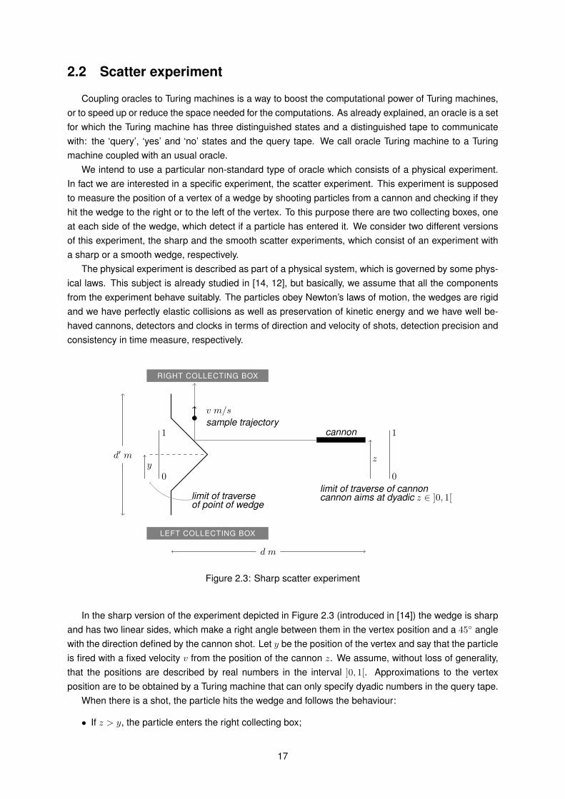
We intend to use a particular non-standard type of oracle which consists of a physical experiment.In fact we are interested in a specific experiment, the scatter experiment. This experiment is supposedto measure the position of a vertex of a wedge by shooting particles from a cannon and checking if theyhit the wedge to the right or to the left of the vertex. To this purpose there are two collecting boxes, oneat each side of the wedge, which detect if a particle has entered it. We consider two different versionsof this experiment, the sharp and the smooth scatter experiments, which consist of an experiment witha sharp or a smooth wedge, respectively.

The physical experiment is described as part of a physical system, which is governed by some phys-ical laws. This subject is already studied in [14, 12], but basically, we assume that all the componentsfrom the experiment behave suitably. The particles obey Newton’s laws of motion, the wedges are rigidand we have perfectly elastic collisions as well as preservation of kinetic energy and we have well be-haved cannons, detectors and clocks in terms of direction and velocity of shots, detection precision andconsistency in time measure, respectively.

RIGHT COLLECTING BOX

LEFT COLLECTING BOX

0

1

y0

1

z

cannon

v m/s

sample trajectory

limit of traverse of cannoncannon aims at dyadic z ∈ ]0, 1[limit of traverse

of point of wedge

d′ m

d m

Figure 2.3: Sharp scatter experiment

In the sharp version of the experiment depicted in Figure 2.3 (introduced in [14]) the wedge is sharpand has two linear sides, which make a right angle between them in the vertex position and a 45◦ anglewith the direction defined by the cannon shot. Let y be the position of the vertex and say that the particleis fired with a fixed velocity v from the position of the cannon z. We assume, without loss of generality,that the positions are described by real numbers in the interval ]0, 1[. Approximations to the vertexposition are to be obtained by a Turing machine that can only specify dyadic numbers in the query tape.

When there is a shot, the particle hits the wedge and follows the behaviour:

• If z > y, the particle enters the right collecting box;

17

• If z < y, the particle enters the left collecting box;

• If z = y, we make no assumptions on the behaviour of the particle.

Remark 2.2.1. So that the third case (z = y) would happen, we would need a dyadic number y, sincez is always dyadic as it is given by a Turing machine. But even then, choosing random positions for thecannon, z, the probability of having z = y is zero, since there are an infinite amount of dyadic numberswithin ]0, 1[ (or any of its subintervals).

We know that unless z = y the particle is detected in a collecting box within a constant time, de-termined by the velocity of the particle v and the distances d and d′ from the cannon to the wedge andbetween the two collecting boxes, respectively. The sides of the wedge make 45◦ angles with the lineof the cannon and then the particle are reflected in a right angle towards a collecting box. Thus, wecan either have the Turing machine waiting the proper amount of time for the result of the experiment,depending on v, d and d′, or set v, d and d′ in such a way that the particle is detected by a collecting boxin the amount of time a Turing machine needs to perform a transition, since that time does not dependon the distance between z and y.

RIGHT COLLECTING BOX

LEFT COLLECTING BOX

0

1

y0

1

z

cannonφ

φ

v m/s

sample trajectory

limit of traverse of cannoncannon aims at dyadic z ∈ ]0, 1[limit of traverse

of point of wedge

d′ m

d m

Figure 2.4: Smooth scatter experiment

In the smooth version of the experiment (introduced in [12]), as depicted in Figure 2.4, we havea smooth wedge. In this case, we do not have a constant time bound as before for the time of theexperiment, the time the experiment takes to run depends on the difference between y and z. When theparticle hits the wedge is reflected as if it hits the tangent line to the wedge at the point of impact, theangle the particle against the wedge makes with the normal to the tangent is the same as the particleagainst the collecting box makes. So, as close to the vertex the particle hits the wedge is as much timeit takes to enter some collecting box. This time is called physical time. In this case, we assume that ifz = y, the particle is reflected backwards and it is not detected in any of the collecting boxes. Note that,here, the collecting boxes are necessarily infinite.

As studied in [12] we know that the physical time taken by the smooth scatter experiment is exponen-tial on |y−z|−1. Lets consider the function g : ]0, 1[→ R such that g(x) describes the shape of the wedgeof a smooth scatter experiment (considering the x axis from left to right). If g(x) is n times continuouslydifferentiable near the vertex position y, with non-zero nth derivative and all the other derivatives until

18

the (n− 1)th vanishing for x = y. Then, with a shot performed at the position z, the time the experimenttakes is t(z), where

A

|y − z|n−1≤ t(z) ≤ B

|y − z|n−1

for some real numbers A, B > 0, when |y − z| is sufficiently small. (see [12] for details)We can then conclude that the physical time of the smooth scatter experiment goes to infinity when z

gets closer to y, being infinite if z = y. Without loss of generality, we assume, for computation purposes,that the smooth scatter experiments we use have a shape, g(x), satisfying the conditions above for n = 2

and that the physical time of the experiment is indeed t(z) = |y− z|−1. We are just setting the constantsto 1.

2.3 Protocol

We intend to use these experiments as oracles to Turing machines. So, we have to explain how is theinformation processed between a Turing machine and an experiment — the communication protocol.

We have three different assumptions on the precision an experiment can set the parameters specifiedby a Turing machine (see [19]).

• The infinite precision, which is when the experiment can set the parameters exactly as the Turingmachine specifies.

• The arbitrary precision, which is when the experiment can commit errors setting the parameters,and the errors can be arbitrarily small and have their limits specified by the Turing machine.

• And the fixed precision, which is when the experiment can commit errors setting the parameters,and the errors have fixed limits, intrinsic to the experiment, that cannot be reduced.

They could also be thought as three different precision assumptions an human technician could setthe parameters for an experiment. We define a different protocol for each different precision assumption.The Turing machine, which aims to use the experiment as an oracle, is modelling a technician, havingto set the parameters for each run of the experiment. Since considering a fixed experiment, which hasa specific vertex position, the only parameter left to set is the cannon position. We must describe howthe Turing machine specifies the cannon position.

To interact with the experiment the Turing machine have a distinguished tape, as well as to interactwith an usual oracle, which is the query tape, and three (or four) additional states, the ‘query’ state (asfor an usual oracle) and the ‘right’ and the ‘left’ states, which can be thought as corresponding to the‘yes’ and ‘no’ states. In some cases of the experiment, mainly in the smooth ones, we may need anotherstate, called ‘timeout’ state, with the purpose of being another possible answer of the experiment as the‘right’ or ‘left’ states, aimed for when the experiment takes too much time and we want to stop it, so wecan keep going with the digital computation on the Turing machine. We may also have to use it to specifythat the particle has hit the vertex in the sharp case of the experiment.

To perform a call to the oracle, when the Turing machine is on its digital computations, writes a wordin the query tape and if it transits to the ‘query’ state, the word in the query tape is used, according to theprotocol (to be defined below), to set the cannon position of the experiment. Afterwards, in the analoguepart (the scatter experiment) a shot is performed and an answer is possibly given by the experimentdetecting the particle in one of its collecting boxes. If the particle is detected in the right collecting box, inthe digital part there is a transition of the Turing machine to the ‘right’ state, and if the particle is detected

19

in the left collecting box, there is a transition to the ‘left’ state. We sometimes couple the analogue-digital machine with the time schedule (mostly in the smooth case), in its digital part, and then if thetime schedule halts before the particle being detected in a collecting box, a transition to the ‘timeout’state occurs. We may need to use a time schedule in the sharp case to decide if the particle has hit thevertex.

As noticed before, we have to specify how the cannon position is specified by the word in the querytape. The cannon position must be a dyadic number in ]0, 1[ since it is given in a finite word to be set ina finite amount of time. Given a word q in the query tape, say q = q1q2 · · · qn (qi is th ith digit of q) wheren = |q|, we consider the real number z = 0.q, i.e. z = 0.q1q2 · · · qn, to describe the cannon position. Aswe work over the binary alphabet (with words over Σ∗) qi is either 0 or 1, and the number z is consideredin its binary representation, we call binary form of z to q1q2 · · · qn. Working for both the sharp and thesmooth experiments, we start to specify the communication protocols already studied concerning timerestrictions ([6, 7, 1]).

Protocol 1.1. Error-free protocolGiven a word q in the query tape, the experiment sets the cannon position to the real number z (usingan infinite precision).

Protocol 1.2. Error-prone arbitrary precision protocolGiven a word q in the query tape, the experiment sets the cannon position, within a uniform distribution,to a real number in the interval ]z − 2|q|, z + 2|q|[ (using an arbitrary precision).

Protocol 1.3. Error-prone finite precision protocolGiven a word q in the query tape, the experiment sets the cannon position, within a uniform distribution,to a real number in the interval ]z − ξ, z + ξ[, where ξ is a fixed positive real number (using a fixedprecision).

With “within a uniform distribution” we mean that a real number in the interval is chosen randomly,having all the numbers the same probability of being chose. A deeper study on distributions to theprecision of physical experiments can be found in [5]. We call accuracy interval, in the error-proneprotocols, to the interval where the experiment chooses the cannon position.

Concerning the error-prone finite precision protocol, without loss of generality, we assume that ξ issmall enough to have the interval ]z − ξ, z + ξ[ embedded in ]0, 1[ at least for z = 1/2. So, we areassuming ξ ≤ 1/2. But sometimes, it might happen that the scatter experiment with fixed precision isused with another cannon positions, when that is the case, we have a more restricted error ξ and theTuring machine only write in the query tape words q which keep ]z − ξ, z + ξ[ embedded in ]0, 1[, wherez = 0.q. We also assume, without loss of generality, for computation purposes, that the fixed error ξ isof the form ξ = 2−N , for some N ∈ N.

Remark 2.3.1. With the error-prone arbitrary precision protocol the length of the accuracy interval isdefined by the size of q, the query word. If we want to shrink the interval keeping its centre, we just needto pad the word q with zeros, and each zero shrinks the interval to the half of its length.

In this case, for some word q with at least one 1, we always have ]z − 2|q|, z + 2|q|[ embedded in]0, 1[. If we want to perform a shot with 0 as lower limit to the accuracy interval, we just have to choosea non-empty query word of the form q = 0 · · · 01 and the accuracy interval is then ]0, 2−(|q|−1)[.

These were the communication protocols already used for the computational bounds of the analogue-digital machine concerning time restrictions. We study space restricted scatter machines with theseprotocols in Chapter 3 and in Chapter 4 we study them for the protocols to be introduced below. Withthe communication protocols between the digital and analogue parts we can introduce properly the

20

machines to be studied throughout the dissertation. For the case of a sharp scatter experiment wecall analogue-digital sharp scatter machine (ShSM for short) to a Turing machine coupled with a sharpscatter experiment as its oracle. We call error-free ShSM to a ShSM with the error-free protocol, error-prone arbitrary precision ShSM to a ShSM with the error-prone arbitrary precision protocol and error-prone finite precision ShSM to a ShSM with the error-prone finite precision protocol. Analogously to thesharp case, for a smooth scatter experiment we call analogue-digital smooth scatter machine (SmSM forshort) to a Turing machine coupled with a smooth scatter experiment. We call error-free SmSM, error-prone arbitrary precision SmSM and error-prone finite precision SmSM to a SmSM with the error-freeprotocol, error-prone arbitrary precision protocol and error-prone finite precision protocol, respectively.

Remark 2.3.2. Throughout this dissertation we use decision scatter machines, which have the ‘accept’and ‘reject’ states but not an output tape. Computation scatter machines could also de used but theyare not interesting for our purposes.

To the time restriction cases these protocols are thought as sufficiently powerful, we see that theseprotocols are equipotent to the new ones which follow (see Proposition 2.3.2), for time restriction cases.But to space restrictions on a scatter machine they may not be sufficient since we are restricting thecannon precision with the space restriction of the query tape. To get a solution on the subject to thepolynomial case, we first thought of consider a communication protocol where the analogue part wouldhave stored the cannon position from the previous shot. Like start to shoot at z = 1/2, and dependingon the result, set the following shot (which is for a future oracle call) at either z = 1/4 or z = 3/4, andso on. With this method we would not need the query tape at all, or we could use it to count the calls tothe oracle or some other purpose. Then, we concluded that this should be equipotent to simply do notrestrict the space of the query tape, which would be a lot simpler to deal with. Since in both methodswe could get access to exponentially long advices in polynomial space, which is sufficient to decide alllanguages (see Proposition 1.2.11).

We have then the ultimate protocol we introduce for the purpose of this dissertation, that is mostlylike the previous one with the exception that, the query tape is even more distinguished. On this newcommunication protocol the query tape is not affected by the space restrictions to the scatter machine,so, we can write as much as we need on the query tape as soon as we use it only to query the oracle (thephysical experiment). The idea of having a tape not affected by the space restrictions to the machineis already used, for example, to the space bounded reducibility (see [3], §3.8). To the space boundedreducibility the machine reducing a set to another has a bound on the space for the work tapes, but theoutput tape is not space restricted. In our case the tape which is not restricted is the query tape. Withthis new protocol, the scatter machine has the same distinguished states to interact with the experimentand distinguished tape, the query tape. The query tape is then restricted in the sense that it must not beused, by the digital part, to perform scratch working. The Turing machine, in its finite control, cannot havethe transition function overusing the query tape. The query tape can only be read to decide either whatto write in itself or when to change to the ‘query’ state. The transition function can then be partitioned intwo parts, a part which can read any tape but can only write in the query tape and transit to the ‘query’state and another part which cannot read the query tape.

All the scatter machines are used satisfying the restrictions to the query tape we just described, andtheir transition functions could be partitioned. They did not need to satisfy that conditions but they wouldnot have any kind of advantage for using the query tape to other than query purposes. But in this lastcase is different, since as the query tape is not space restricted, use it for scratch computations couldboost the computational power of the digital component of the analogue-digital machine.

We then introduce the three communication protocols (for the three precision assumptions) betweenthe analogue and the digital parts. The protocols are exactly the same once the query word is given, the

21

difference is in the length properties of the query word.

Protocol 2.1. Error-free protocolGiven a word q in the query tape, the experiment sets the cannon position to the real number z.

Protocol 2.2. Error-prone arbitrary precision protocolGiven a word q in the query tape, the experiment sets the cannon position, within a uniform distribution,to a real number in the interval ]z − 2|q|, z + 2|q|[.

Protocol 2.3. Error-prone finite precision protocolGiven a word q in the query tape, the experiment sets the cannon position, within a uniform distribution,to a real number in the interval ]z − ξ, z + ξ[, where ξ is a fixed positive real number.

We call standard communication protocol to the first protocol we specified, already used in [6] for ex-ample, and we call space-generalized communication protocol (or generalized communication protocol)to this last one we just specified. We have the same designations for the scatter machines with this newprotocol as we have with the other one. We call analogue-digital sharp scatter machine (ShSM for short)and analogue-digital smooth scatter machine (SmSM for short) to a Turing machine coupled with a sharpor a smooth scatter experiment, respectively. We call error-free ShSM, error-prone arbitrary precisionShSM and error-prone finite precision ShSM to a ShSM with the error-free protocol, error-prone arbitraryprecision protocol and error-prone finite precision protocol, respectively. The same is to the case of aSmSM, we have the error-free SmSM, the error-prone arbitrary precision SmSM and the error-pronefinite precision SmSM. We call, when not already clear, standard analogue-digital scatter machine orgeneralized analogue-digital scatter machine to distinguish between them.

Concerning the differences between the two protocols we can always obtain the results from a stan-dard scatter machine on a generalized scatter machine. We only need to simulate the standard scattermachineM on a generalized scatter machine with an additional tape, whereM′ (the generalized scattermachine) writes on that tape exactly what it writes in the query tape. Then, when M reads the querytapeM′ reads the additional tape and obtain exactly the same information. Leading us to the followingProposition:

Proposition 2.3.1. If a standard scatter machine can decide a set A ∈ Σ∗, then there is a generalizedscatter machine that decides the set A.

The result holds for either the sharp or the smooth scatter machines, with any precision assumptionand for any constraints to the scatter machine (time or space bounds, for example). The reciprocal isnot true as we conclude through the dissertation (see Propositions 3.6.4 and 4.1.1).

Proposition 2.3.2. Concerning scatter machines without space restrictions, a set A ∈ Σ∗ is decidableby a generalized scatter machine if and only if is decidable by a standard scatter machine.

Proof. By Proposition 2.3.1 we have that a set decidable by a standard scatter machine is decidable bya generalized scatter machine.

If a set A ∈ Σ∗ is decidable by a generalized scatter machineM which is not space restricted, then astandard scatter machineM′, behaving likeM, can use exactly the same queriesM uses in any of itscomputations. Since the query tape ofM′ is not space restricted as well as any other tape in eitherM′

orM. Therefore, a standard scatter machine can decide all the sets that a generalized scatter machinecan, and the desired equivalence follows.

As a corollary, of course, if a scatter machine is clocked in polynomial time (it is not space restricted),both the standard and the generalized protocols lead to the same results.

22

2.4 Scatter machine

The analogue-digital scatter machine, as described earlier, consists of coupling a Turing machinewith a scatter experiment. We specified, for the three different precision assumptions, two communica-tion protocols between the two components of the scatter machine, the analogue and the digital parts.We then got, for each one between the standard and the generalized protocols, an error-free protocoland two error-prone ones. With the error-free protocol (infinite precision) we have a deterministic exper-iment, in the sense that two runs with the same parameter z, the specified cannon position, always havethe same result. But with the error-prone protocols (arbitrary and fixed precisions), if we have the vertexposition inside the accuracy interval, we have a non-deterministic experiment, we may have differentresults in two calls with the same parameter z. We have then two different kinds of scatter machine, forwhich we should define decidability of languages, the deterministic and the probabilistic kind.

We always consider a deterministic Turing machine as the digital component for a scatter machine,its possible probabilistic behaviour is always provided by the experiment (see Proposition 2.4.1). Wecan use an error-prone protocol to get a deterministic scatter machine, we just have to be careful toguarantee that no call of probabilistic answer is made, as it actually happens on the lower bounds whenwe want to find the advice with the arbitrary precision (see Propositions 3.6.2 and 3.7.2).

For a deterministic scatter machine, as we have for a deterministic Turing machine, we say that aword w ∈ Σ∗ is accepted if the scatter machine halts the computation for the input w in the ‘accept’ state.

Definition 2.4.1. We say that a deterministic scatter machineM decides a set A ⊆ Σ∗, if for all w ∈ Σ∗,M accepts w if and only if w ∈ A.

For a probabilistic scatter machine, we use the bounded error probability decision criterion (seeDefinition 1.2.1).

Definition 2.4.2. We say that a probabilistic scatter machine M decides a set A ⊆ Σ∗ if, there is arational number ε with 0 < ε < 1/2 such that, for every w ∈ Σ∗ (a) if w ∈ A, then M rejects w withprobability at most ε and (b) if w /∈ A, thenM accepts w with probability at most ε.

It is the same decision criterion as to define BPP or BPPSPACE . We say that a probabilistic scattermachine accepts a word w ∈ Σ∗ if it halts the computation for the input w in the ‘accept’ state. But if werun the same probabilistic scatter machine on w twice, it is possible to have w accepted exactly once.Given these definitions, we have a bounded error probabilistic scatter machine, but we call it probabilisticscatter machine, as we do for the bounded error probabilistic Turing machines through the dissertation.

The probabilistic uniform class BPP has the property that given a set A ∈ BPP , witnessed by aprobabilistic Turing machine M with constant ε, we have a probabilistic Turing machine (based on M)that decides A with error probability at most 2−p(n) for each input w with |w| = n. Analogously as to theclass BPP , we assume the same result for general probabilistic scatter machines, since as the prooftechnique consists in running the Turing machine enough times we can do the same with the scattermachines. We use the assumption, without loss of generality, that a probabilistic scatter machine has itsbounded error less or equal to 1/4.

Remark 2.4.3. If a probabilistic scatter machine has a deterministic behaviour and decides a set A ⊆Σ∗ with the deterministic criterion, then it also decides A with the bounded error probability decisioncriterion. Since if a word w ∈ A, the machine rejects w with probability 0 < ε, and if w /∈ A, the machineaccepts w with probability 0 < ε.

With respect to the lower bounds we may need to simulate a probabilistic advice Turing machine ona scatter machine, this subject was already discussed in [6, 8, 9]. It would be easy to just consider a

23

probabilistic Turing machine in the digital part of the scatter machine to the effect, but we can do it in adifferent way, more elegant and appropriate to the power of the scatter experiment.

First, we have to notice that a scatter experiment with an error-prone protocol can be used as a coin.If we consider a cannon position close enough to the vertex position so that the vertex position would beinside the accuracy interval, we have a probabilistic experiment with two or three possible answer caseswith probability greater than zero (depending on if we have a sharp or a smooth experiment). We canalways consider the union of some answer cases in order to have two hypothesis with complementaryprobability values. With the arbitrary precision assumption we can always use the query q = 1 whichproduces the accuracy interval ]0, 1[ to have a probabilistic coin toss. With the fixed precision assumptionwe can choose a query word that gets the vertex position inside the accuracy interval based on the vertexposition and the fixed error of the protocol, resulting in a probabilistic coin toss. In both cases we canobtain an interval ]δ, 1 − δ[, for some δ with 0 < δ < 1/2, that has at least one of the complementaryprobability values inside it.

It may happen that we obtain a fair coin toss from the scatter experiment, but generally, we obtain abiased coin toss. We have a result, already stated in [1] for example, that states that a biased coin canbe used to generate a sequence of fair coin tosses of length n.

Proposition 2.4.1. Given a biased coin with probability of heads p ∈ ]δ, 1 − δ[, for some δ with 0 < δ <

1/2, and a real number λ ∈ ]0, 1[, we can generate a sequence of independent fair coin tosses of lengthn with a linear amount of biased coin tosses on n, up to probability λ.

We can then simulate a probabilistic Turing machine with a probabilistic scatter machine. If we havea scatter machine bounded in polynomial space we may need to have a sequence of 2n independent faircoin tosses. We cannot generate them all at once since we cannot write a sequence of length 2n as weare bounded in polynomial space. If we generate one fair coin toss at a time, we need each probabilityof success greater than 1 − 2−n−4 in order to have the probability of success for all the 2n coin tossesgreater than 1 − 2−4, for example. We need then an exponential amount of unfair coin tosses (calls tothe oracle) to obtain each fair coin toss (see [6], §7, Lemma 7.7). As we can use the smooth scatterexperiment with a constant time schedule and the sharp one has already a constant physical time, wedo not need more than an exponential time to generate all the 2n fair coin tosses.

With respect to the upper bounds, we need to simulate the probabilistic answers from the oracle ona probabilistic Turing machine, the subject is already discussed in [7]. For each call to the oracle that wemay need to simulate, we must have the probability of the answers from the oracle as dyadic rationals,otherwise it would not be possible to simulate them on a general probabilistic Turing machine.

We do not have a probabilistic scatter experiment with the infinite precision assumption, we onlyhave it when using the error-prone protocols. Based on the behaviour we assume for the error-proneprotocols we always have an accuracy interval centred on z (where z = 0.q and q is the query word) withdyadic boundaries z − 2−N and z + 2−N , for some N ∈ N.

Given a dyadic number with polynomially sized representation (a dyadic vertex position for example)we can check in polynomial time whether it is inside the accuracy interval or not. When we alreadyknow that the answer from the oracle is probabilistic, i.e. (in the sharp case) the dyadic vertex positionyd

is inside the accuracy interval or (in the smooth case) at least one of the boundary numbers is (seeSection 3.5), we can (in the sharp case) compute both the probability for the answer being left and right,which correspond to y

d− (z − 2−N ) and z + 2−N − y

d, respectively. Thus, we can simulate digitally

an event with probability (yd− (z − 2−N ))/2−N+1 to simulate the oracle call (see [7]). Analogously, in

the smooth case we can simulate, if necessary, an event with three possible outcomes, each one withdyadic probability. We can use a fair coin toss to produce any event with dyadic probability, which takes

24

n units of time where n comes from the dyadic probability k/2n, for some k with 0 ≤ k ≤ 2n (n is linearon the dyadic number representation). We can also use fair coin tosses to produce a probabilistic eventwith three possible outcomes, as for example using two coin tosses. Of course we assume that on ageneral probabilistic Turing machine, we have a fair coin toss which takes exactly one transition.

The cost for the computations needed above is polynomial on the size of the dyadic number repre-sentations. So, if we have polynomially sized representations for y

d, z and 2−N , which we do if we have

polynomially sized words q and describing yd, all the simulation takes a polynomial time. The same is,

in the smooth case, with polynomially sized representations for the dyadic boundary numbers.

25

Chapter 3

Standard scatter machine

Throughout this chapter we intend to study the computational power of the scatter machine boundedin polynomial space with the standard communication protocol. We stablish the computational power forboth the sharp and the smooth scatter experiments with any of the three precision assumptions.

At first we present auxiliary results needed in the proofs and only then the proofs itself. This com-munication protocol between the analogue and the digital part is the protocol used for the study of thescatter machine bounded in polynomial time. Here we adapt the results obtained in [6, 7, 13] to the caseof bounded space.

We can start with noticing that the scatter machine bounded in polynomial space can decide all thesets that the scatter machine clocked in polynomial time decide. Since a scatter machine clocked inpolynomial time cannot use more than a polynomial space, the scatter machine bounded in polynomialspace can simulate any scatter machine clocked in polynomial time, because a scatter machine boundedin polynomial space can use an exponential amount of time (see Proposition 3.4.1).

We conclude then that the complexity classes that a scatter machine clocked in polynomial compute(see [10]) are at least embedded in the lower bounds for the scatter machine bounded in polynomialspace.

We can state then the following lower bounds for the analogue-digital sharp scatter machine boundedin polynomial space:

Infinite Arbitrary Fixed

Lower Bound P/poly P/poly BPP// log ?

Table 3.1: Standard communication protocol ShSM

And we can state the following lower bounds for the analogue-digital smooth scatter machine boundedin polynomial space:

26

Infinite Arbitrary Fixed

Lower Bound P/ log ? BPP// log ? BPP// log ?

Table 3.2: Standard communication protocol SmSM

The proof techniques presented below are adaptions from the techniques used to proof the resultsabove, as well as other results concerning computational power of analogue-digital machines.

3.1 Vertex position

In this section we present a useful coding to proof the lower bounds of the computational power ofthe scatter machine. With the aim of simulate an advice Turing machine on a scatter machine, we shouldbe able to code the information of an advice function in the vertex position.

To code a prefix advice function as a vertex position

• We consider the function c : Σ∗ → Σ∗, where the encoding c(w) is obtained from the word w ∈ Σ∗

by replacing every 0 by 100 and every 1 by 010.

• Given a prefix advice function f , we consider the function x(f) : N → Σ∗ such that x(f)(n) =

c(f(n)).

• We call x(f) to the limit sequence(1) of x(f).

• And finally, we define the real number y ∈ ]0, 1[ such that y = 0.x(f).

We can then place the vertex of a scatter experiment at y.

Example.c(ε) = ε.If f(0) = 0 1 0 0 1 1 then x(f)(0) = c(f(0)) = 1 0 0 0 1 0 1 0 0 1 0 0 0 1 0 0 1 0 ,x(f) = 1 0 0 0 1 0 1 0 0 1 0 0 0 1 0 0 1 0 · · · and y = 0.1 0 0 0 1 0 1 0 0 1 0 0 0 1 0 0 1 0 · · · .

We use the encoding c so that we would not have to distinguish between the two possible binaryexpansions of dyadic(2) rationals. No dyadic rational can occur as an y = 0.x(f), since x(f) was con-structed not to have the occurrence of 0000 or 1111, and a dyadic number would have its binary expan-sion ending in either all zeros or all ones. As for example, 1/2 has the two possible binary expansions0.10000 · · · and 0.01111 · · · . This ambiguity (over Σ∗) is limited to the dyadic rationals, any other realnumber has a unique binary expansion.

The numbers which can occur as an y = 0.x(f) are all elements of the so-called Cantor Set. This kindof codification is often used to distinguish between close values. The Cantor Set has been considered toboost computation in the neural net framework as in [20, 21] and in other computational models workingwith real valued parameters such has in [15, 23].

To find f(n) from x(f), when f is a prefix advice function, we read the digits of x(f) in triples.Whenever the triple 100 is read we have a 0 in the advice and whenever the triple 010 is read we

(1) The limit sequence of x(f) is the infinite word over Σ∗ for which any x(f)(n) is a finite prefix of it.(2) A dyadic number is a rational of the form n/2m for some n ∈ Z, m ∈ N.

27

have a 1. When dealing with a prefix advice function f ∈ poly , as we have a polynomial p such that|f(n)| < p(n), it is enough to consider the first 3 · (p(n)− 1) digits of x(f). As we can consider f ∈ poly

as an advice function of known size, we can easily get exactly f(n) from x(f) and no more than that.To find x(f) by means of the scatter experiment, the Turing machine applies the linear search method.

This is a linear search method with additional information we have about the vertex position. We knowthat either y = 0.100 · · · or y = 0.010 · · · , so, if we set the cannon to shoot in the middle, at z = 0.011,then if the answer is right it is because y < z and if the answer is left it is because y > z. The first digitof the advice is then known, i.e. the first triple of x(f). To get the ith digit of the advice, having read thefirst i−1 digits, we set the cannon at z = 0.x(f)1x(f)2 · · ·x(f)i−1011, where x(f)i is the ith triple in x(f)

and follow the same reasoning.This search method leads us to the following algorithm:

Algorithm 1: Linear search methodData: Number of triples we want, mSet q′ := ε ;while |q′| < 3 · n do

Make an oracle call with the query word q = q′011 ;if The answer from the oracle is right then

Set q′ := q′010 ;endif The answer from the oracle is left then

Set q′ := q′100 ;end

endreturn q′ (q′ is a prefix of x(f))

Remark 3.1.1. When a scatter machine is using this linear search method the query coincide with x(f)

but at the last three digits.

The method described needs a space equal to three times the size of the advice, which is polynomialon the size of the input for a polynomial advice. Also, in the sharp case of the experiment the sameamount of time is enough, since we need to perform a call to the oracle for each digit of the advice andthe oracle calls take a constant time. In the smooth case we need an exponential amount of time on thequery size for each call to the oracle. To obtain m triples of x(f) we need less than 23m+3 units of time,since as at the ith call |y− z| > 2−3i−2, we conclude that the ith call needs at most 23i+2 units of time tobe answered.

If we consider an exponential advice, as with the generalized communication protocol, we need anexponential space to write the query, and as we need to perform an exponential amount of queries toobtain the advice we need an exponential amount of time even for the sharp scatter machine. In thesmooth case we need a time with magnitude order of 22n

(see Propositions 4.2.2 and 4.2.3).

Proposition 3.1.1. Let q be a query to the linear search method of a scatter machine with vertex positiony = 0.x(f), for some prefix advice function f . The error-prone arbitrary precision scatter experiment,with the precision set to at least 2−|q|−3, has the same result as the error-free scatter experiment. In thesmooth case of the experiment, the time is at most doubled.

Proof. Since with the linear search method, the scatter experiment is set to fire the cannon at a distanceof at least 2−|q|−2 from the vertex position, if we set the error to be at most 2−|q|−3, the shot is performed

28

at at least 2−|q|−3 from the vertex position, on the same side. So, we have the same answer from theoracle.

In the smooth case, with |y− z| > 2−|q|−2 we had the time to get an answer bounded by 2|q|+2. Now,with |y − z| > 2−|q|−3 we have the time bounded by 2|q|+3, which is twice as much.

Remark 3.1.2. The time in the smooth case can also be reduced by a third. In the error-prone case(arbitrary precision), we have to pad the query word q with three 0’s in order to get the desired accuracyinterval, and to use the linear search method is not necessary to increase the number of oracle calls.

For the proof of the upper bounds, as explained below (see Section 3.3), the scatter machine mayhave a vertex position not in the Cantor set. The scatter machine then needs a measurement algorithmto a more general case, this subject is already studied in [11]. An analogous algorithm to the specifiedone for determining a digit of the binary form of the vertex position at a time would suffice, and wouldalso work only with non-dyadic vertex positions.

An important result on the subject is that an analogue-digital machine, with a general linear searchmethod, can measure any measurable real valued parameter that could be measured by any analogue-digital algorithm (see [11]).

3.2 Find the vertex position with fixed precision

With the fixed precision assumption we must use a different technique, since with a fixed precisionwe are only able to approximate the vertex position until a finite amount of digits. We make then use ofthe Chebyshev’s inequality to obtain an accurate enough approximation of the vertex position.

Proposition 3.2.1. Let z ∈ ]0, 1[ be a real number and y = 0.x(f) a number in the Cantor Set, for someprefix advice function f . If |y − z| < 2−n−5 then the first n digits of the binary form of z and y coincide.

Proof. If at least one of the first n digits of the binary expansion of z and y differ, lets assume that the ith

digit is different and the previous i− 1 are equal, for 1 ≤ i ≤ n. Then, in the worst case scenario, eitherzi = 1 followed by a sequence of 0’s and yi = 0 followed by a sequence of 1’s, or zi = 0 followed by asequence of 1’s and yi = 1 followed by a sequence of 0’s. Where zi and yi are the ith digit in the binaryform of z and y, respectively. In any of the two cases, as y = 0.x(f) for some prefix advice function f ,the sequence of 0’s or 1’s in y has at most 3 digits and thus, we conclude that |y − z| ≥ 2−i−5. So, if|y − z| < 2−n−5, then the first n digits of the binary form of z and y are equal.

A scatter machine must then find a real number close enough to the vertex position so that the firstwanted amount of digits from both numbers are equal.

Proposition 3.2.2. Given a prefix advice function f , an error-prone finite precision ShSMM can obtainm triples of x(f) with error probability smaller than 2−c with 26m+8+c oracle calls.

Proof. Note that if y′ = 1/2 + ξ − 2ξy is the vertex position of M, where y = 0.x(f) and ξ is the fixederror of the protocol, and the cannon position is set at z = 1/2, then the particle has probability y ofbeing detected in the right collecting box.

Let R be the number of particles detected in the right collecting box after s shots, we can then esti-mate y as R/s. So that we could apply Proposition 3.2.1 we want s such that |y−R/s| < 2−3m−5. SinceR is a random variable with expected value µ = sy and variance(3) σ2 = sy(1 − y), using Chebyshev’sinequality, we conclude that Pr(|µ − R| ≥ kσ) ≤ k−2, for any k ∈ R+. Considering k = 2−3m−5sσ−1,we obtain Pr(|y − R/s| < 2−3m−5) > 1 − 26m+10s−1y(1 − y). As y(1 − y) ≤ 2−2, since y ∈ ]0, 1[, if weconsider s = 26m+8+c, we get Pr(|y −R/s| < 2−3m−5) > 1− 2−c.(3) Of course, σ is the positive value such that σ2 = sy(1− y).

29

To obtain the first |f(n)| triples of x(f) with error probability smaller than δ we should choose c suchthat 2−c ≤ δ and perform 26|f(n)|+8+c oracle calls.

If f ∈ poly , we need an exponential amount of oracle calls on n. So, to write and read R and s andto compute R/s until 3 · |f(n)| digits, we need a polynomial space on n. An exponential time on n isenough, since there is a division algorithm that runs in polynomial time.

Proposition 3.2.3. Given a prefix advice function f , an error-prone finite precision SmSMM can obtainm triples of x(f) with error probability smaller than 2−c with 26m+8+c oracle calls.

Proof. Note that, if y′ = 1/2 + ξ − 2ξy is the vertex position ofM, where y = 0.x(f) and ξ is the fixederror of the protocol, and the cannon position is set at z = 1/2, then the particle has probability y of beingdetected in the right collecting box. As we are using the smooth case of the experiment, if we use thetime schedule, we have three possible outcomes with probability greater than zero. For any fixed timeschedule T , there is a number η ∈ ]0, 1] such that, if the shot z = 1/2 is performed within ]y′ − η, y′ + η[,the time schedule halts before the oracle gets to an answer. We want η < 2ξ(1 − y) and η < 2ξy sothat the interval ]y′ − η, y′ + η[ would be embedded in ]1/2 − ξ, 1/2 + ξ[. Since 1/4 < y < 5/8, as yis of the form 0.x(f) for some prefix advice function f , it is enough to consider a time schedule whichmakes η < ξ/2, a constant time schedule is enough. So, the probability of the particle being detectedin the right collecting box before the time schedule halts is (2ξy − η)/2ξ, and the probability of the timeschedule halts before the particle being detected in some collecting box is η/ξ.

Considering the time schedule T in use. Let R be the number of particles detected in the rightcollecting box before the time schedule halts after s shots and U the number of particles that were notdetected in any of the collecting boxes until the time schedule halts, after the same s shots. We can thenestimate y as (R+ U/2)/s = (2R+ U)/2s.

So that we could apply Proposition 3.2.1, we want s such that |y − (2R + U)/2s| < 2−3m−5. As2R + U is a random variable with expected value µ = 2sy and variance σ2 = s(4y(1 − y) − η/ξ), usingChebyshev’s inequality, we conclude Pr(|µ − (2R + U)| ≥ kσ) ≤ k−2, for any k ∈ R+. Consideringk = 2−3m−4sσ−1, we obtain Pr(|y − (2R + U)/2s| < 2−3m−5) > 1 − 26m+8s−1(4y(1 − y) − η/ξ). As3/4 < 4y(1 − y) ≤ 1 and 0 < η/ξ < 1/2 since 1/4 < y < 5/8 and 0 < η < ξ/2, respectively. If weconsider s = 26m+8+c, we get Pr(|y − (2R+ U)/2s| < 2−3m−5) > 1− 2−c.

To obtain the first |f(n)| triples of x(f) with error probability smaller than δ we should choose c suchthat 2−c ≤ δ and perform 26|f(n)|+8+c oracle calls.

If f ∈ poly , we need an exponential amount of oracle calls on n. So, to write and read R and s

and compute R/s until 3 · |f(n)| digits, we need a polynomial space on n. An exponential time on n isenough, since there is a division algorithm that runs in polynomial time.

From the results stated in the last two Propositions we can conclude that for the fixed precisionprotocol, both the sharp and the smooth scatter machines can obtain the same information with thesame error probability for a sufficiently centred vertex position.

30

3.3 Sparse oracles

As described above to the lower bounds, we construct the vertex positions so that they would notbe dyadic numbers. To the upper bounds, as in general, the vertex of a scatter experiment can happento be placed at dyadic positions. We use here proof techniques, not as simple as the to the lowerbounds, for which we need to introduce some other concepts. We aim to simulate scatter machines ingeneral advice Turing machines, where we use the advice to answer the oracle calls. With the standardcommunication protocol we only need to simulate polynomially sized oracle calls, since we are studyingscatter machines bounded in polynomial space.

Concerning the sharp scatter experiment, in the error-prone protocols we assume that if the particlehits the vertex, it deterministically enter the same collecting box (the right or the left one). The proofsare analogous to other assumptions, we could just have to use ternary trees instead of binary ones. Weuse the same proof technique for any of the precision assumptions with te smooth scatter experiment,but in this case we always need ternary trees. With the error-free protocol (sharp scatter experiment)we use a different proof method analogous to the one in [6]. We do not need to assume what happenswhen the particle hits the vertex, but we do have to assume that the behaviour is also deterministic i.e.if the particle hits the vertex, the same result always happens.

To code a vertex position as a sparse oracleGiven a real number y ∈ ]0, 1[, considered with its binary expansion in the terminating form (i.e. 0.01

instead of 0.001111 · · · ), and an increasing total function f : N → N, we construct a sparse(4) set. Forexample, lets consider y = 0.0110001010110100 · · · and the polynomial function f(n) = (n+ 1)2.

To construct the set Ofy , first we consider the infinite word over Σ∗ that represents the binary form ofy, possibly ending in all zeros, and then, after each f(n) digits in the infinite word, we append either thesymbol ‘=’ or the symbol ‘>’, depending on if y is equal to its binary expansion truncated at that point ornot, respectively.

In our example, we would get, 0>110>00101>0110100= · · · or 0>110>00101>0110100> · · · , de-pending on if the binary form keeps on with all zeros or not, respectively. Since f(0) = 1, f(1) = 4,f(2) = 9 and f(3) = 16, for the function chose as example (f(n) = (n + 1)2). Note that the digitf(n) + n+ 1, for any n ∈ N, in any word from Ofy is always a ‘>’ or ‘=’ sign.

If an ‘=’ sign appears, we know that from there on, no 1 ever occurs again and only the symbol ‘=’occurs besides the zeros. We consider the set Ofy as the set with all (finite) prefixes of the resultingword. Ofy is clearly a sparse set (it can even be seen as a tally(5) set).

Proposition 3.3.1. PSPACE/poly =⋃O sparse PSPACE (O).

Proof. First, lets assume A ∈ PSPACE/poly . If A ∈ PSPACE/poly , there exists B ∈ PSPACE and anadvice function f ∈ poly such that, for every w ∈ Σ∗, w ∈ A if and only if 〈w, f(|w|)〉 ∈ B. LetMB be anadvice Turing machine which decides B in polynomial space.

Let O be the set {〈0n, x〉 ∈ Σ∗ : x is a prefix of f(n)}. O is a sparse set since, for any n ∈ N, O hasat most n words of size n. Since for any n ∈ N and k ∈ {0, 1, . . . , n− 1}, there is at most one prefix x off(k) that makes

⟨0k, x

⟩with size n.

Consider the oracle Turing machine M, which for an input w, uses the usual oracle O to obtain⟨0|w|, f(|w|)

⟩(see [3], Chapter 5, Theorem 5.26). Afterwards, M simulates MB over 〈w, f(|w|)〉 and

accepts w if and only ifMB accepts 〈w, f(|w|)〉. Thus,M decides A. As to get⟨0|w|, f(|w|)

⟩and write

〈w, f(|w|)〉 a polynomial space on |w| is enough, and also, to simulateMB on 〈w, f(|w|)〉 a polynomial

(4) A set is sparse if it has at most p(n) words of length n, ∀n ∈ N, for some polynomial p.(5) A set is tally if it has at most one word of length n, ∀n ∈ N.

31

space on | 〈w, f(|w|)〉 |, which is polynomial on |w|, is enough. We can conclude that M operates inpolynomial space on |w| and so, that A ∈ PSPACE (O).

The computation time of M on w is the time that MB needs for the input 〈w, f(|w|)〉 plus the timeneeded to get

⟨0|w|, f(|w|)

⟩and write 〈w, f(|w|)〉. Except for the simulation, this time is polynomial on

|w|.Now, conversely, lets assume A ∈ PSPACE (O), for some sparse set O. So, there is an oracle Turing

machineM which decides A in polynomial space p with the usual oracle O.Let mn ∈ N be the number of words of length n in O, so, as O is sparse, there is a polynomial q such

that mn ≤ q(n), for any n ∈ N. Let also the words wn1 , wn2 , . . . , wnmnbe all the words of length n in O.

And let finally f be the advice function such that

f(n) = w11#w1

2# · · ·#w1m1

#w21#w2

2# · · ·#w2m2

# · · ·#wp(n)1 #w

p(n)2 # · · ·#wp(n)

mp(n)

f ∈ poly since, as mi ≤ q(i), for any i ∈ N, we have f(n) ≤∑p(n)i=1 (i + 1)q(i) − 1 which is a polynomial

on n.Consider the advice Turing machine M′, which for an input 〈w, f(|w|)〉, behaves exactly like M for

the input w except when the oracle calls. Where for a query q uses the advice f(|w|) to give the sameanswer as the oracle (if q is in f(|w|) answers yes, otherwise answers no). For an input w, M canonly write in the query tape a word q with |q| ≤ p(|w|). So, M′ can answer any query it may needfor a computation of M. We conclude then that M′ accepts 〈w, f(|w|)〉 if and only if M accepts w.To simulate M on w, M′ needs a polynomial space on | 〈w, f(|w|)〉 |, since M is space bounded by apolynomial, and to have the answers from the oracle, M′ would need no further space. Therefore, weconclude that A ∈ PSPACE/poly .

The computation timeM′ takes on 〈w, f(|w|)〉 is the same timeM takes on w plus the time neededto get the answers from the oracle. Except for the simulation, this time is polynomial on |w|.

With this last result we use a sparse oracle like Ofy to prove the upper bound for the error-free ShSM(Proposition 3.6.4). Given an oracle Turing machine, with oracle Ofy for some increasing total function fand real number y ∈ ]0, 1[, to find the word of size n in Ofy (Ofy is a tally set), it must find al the smallerwords in Ofy since they are a prefix of the wanted word. Lets call di to the ith digit of the word. To findthe ith digit of the word, when already known the first i− 1 digits, the oracle Turing machine must querythe oracle with the word d1d2 · · · di−10 and conclude the ith digit is 0 if and only if the answer is yes; ifi 6= f(j) + j + 1 for any j ∈ N. If i = f(j) + j + 1 for some j ∈ N (and the first i − 1 digits are known);the oracle Turing machine must query the oracle with the word d1d2 · · · di−1 > and conclude the ith digitis > if and only if the answer is yes.

We need an increasing function f so that the condition i = f(j)+j+1 for some j ∈ N can be decidedby a Turing machine.

32

3.4 Probabilistic trees

As already discussed in Chapter 1, we can see the computation tree of a Turing machine as a binarytree. In the case of a scatter machine, if we consider an experiment with two possible answers, wecan still see its computation tree as a binary tree, but if we consider an experiment with three possibleanswers we have to consider a ternary tree for its computation tree. For the sharp cases, we areassuming that we have just two possible answers. Even if we would consider three possible answers,one of them would always be assigned with probability zero.

Concerning the depth of the computation trees, which is a relevant subject to the upper bound prooftechniques, we can use an analogous reasoning to proof of Proposition 2.1.2 to state that the depth ofa computation tree of an analogue-digital machine bounded in polynomial space is at most exponential.Note that the bound we give there to the possible number of configurations is not possibly to accomplish,i.e. we do not have as much configurations to reach in the same computation of the Turing machine.Here, to avoid unnecessary constants, we say that the limit to the depth of an analogue-digital machinebounded in polynomial space p is 2p(n) for an input of size n. For a different limit, also exponential, allthe results would be analogous, possibly with different constants but keeping the same magnitude order.

Proposition 3.4.1. An analogue-digital machine bounded in polynomial space p, for an input of size n,has the depth of its computation tree limited by 2p(n).

A probabilistic tree is a weighted tree where the sum of the weights of the edges from the same parentis one. Given a tree T , an assignment of probabilities for T , α, is a map α : ET → [0, 1], where ET is theset of edges of T , that assigns a probability to each edge of T , making T into a probabilistic tree. Wecall T α to the this probabilistic tree and ρ(T ) to the set of all possible assignments of probabilities for T .

Given a rooted tree, we call total path to a path from the root to a leaf of the tree, and given aprobabilistic rooted tree, we call probability of the total path to the product of the weights along the path.

Note that given a rooted tree T , we can consider a collection of total paths from T , having then arooted subtree of T (Ts).

Definition 3.4.1. Given a probabilistic rooted tree T α, consider any weighted rooted tree consisting ona collection of total paths from T α and call it T αs . We say that the probability of T αs , denoted by P (Ts, α),is the sum of the probabilities of the total paths of T αs , for all its total paths.

Remark 3.4.2. Given a probabilistic rooted tree T , if we consider the subtree Ts consisting of all its totalpaths, then P (Ts, α) = 1. P (T , α) is always 1.

We denote by Tn,m the set of all n-ary rooted trees of height less or equal to m.Given a tree T , we define a distance among the assignments in ρ(T ), which we denote by dT (or

usually just d). This distance is given by the maximum of the absolute values of the differences of theprobabilities over each edge. Given α, α′ ∈ ρ(T )

dT (α, α′) = max{|α(e)− α′(e)| : e ∈ ET }.

We can then define a set of useful functions.

Definition 3.4.3. Given n ∈ N+, we define the function fn : N× [0, 1]→ [0, 1] as

fn(m, k) = maxT ∈Tn,m

sup{|P (T , α)− P (T , α′)| : ∀α, α′ ∈ ρ(T ) : dT (α, α′) ≤ k}.

Remark 3.4.4. For a n-ary rooted tree T of depth less or equal to m, if d(α, α′) ≤ k, for all α, α′ ∈ ρ(T ),then |P (T , α)− P (T , α′)| ≤ fn(m, k).

33

Proposition 3.4.2. f2(m, k) ≤ 2mk.

Proof. See [7], §2, Proposition 2.1.Or this is an immediate corollary of Proposition 3.4.4, since 2− 1 < 2.

Proposition 3.4.3. Let M be an error-prone (arbitrary or finite precision) ShSM that decides the setA ⊆ Σ∗ in polynomial space p, with error probability ε ≤ 1/4. If M′ is an error-prone ShSM that, foran input w with |w| = n, behaves exactly like M except when the oracle calls. Where for any call, theprobability of the answer differs at most 2−p(n)−4. Then,M′ decides A with error probability ε′ ≤ 3/8.

Proof. Given a word w ∈ Σ∗, consider the computation tree Tw of M for the input w,(6) and let α, α′ ∈ρ(Tw) be the assignments that give to the edges of Tw the probabilities given by the experiments ofM and M′, respectively. Consider the subtree of Tw consisting on all the total paths from Tw thatcorrespond to a wrong computation(7) ofM when deciding A, and call it T ×w .

As M is space bounded by the polynomial p, for an input w, the depth of Tw is limited by 2p(|w|)

(see Proposition 3.4.1), and as we considered Tw as a binary tree. Using Proposition 3.4.2, since then|P (T ×w , α) − P (T ×w , α′)| ≤ f2(m, k) ≤ 2mk, where m and k are the depth and the biggest difference forany probability of T ×w , respectively, we have

P (T ×w , α′) ≤ P (T ×w , α) + |P (T ×w , α)− P (T ×w , α′)|

≤ ε+ 2 · 2p(n) · k

≤ 2−2 + 2p(n)+1k.

So, if we have k such that 2p(n)+1k ≤ 2−3, we get P (T ×w , α′) ≤ 3/8. Therefore, for any word w ∈ Σ∗,M′

make the same decision asM with error probability ε′ ≤ 3/8 instead of 1/4.

Concerning Proposition 3.4.2 we can also get a more general result. Needed in the dissertation tothe smooth scatter experiment cases, since we need ternary trees instead of binary ones. This result isalready stated in [1, 5].

Proposition 3.4.4. fn(m, k) ≤ (n− 1)mk.

Proof. The proof follows by induction on m. The result is valid for m = 0, since the only tree in any ofthe sets Tn,0 has zero edges.

Lets then assume that fn(m, k) ≤ (n−1)mk and proof that fn(m+ 1, k) ≤ (n−1)(m+ 1)k. Considera tree T ∈ Tn,m+1, and lets see it as a root, n edges from the root, e1, e2, . . . , en, and n trees in Tn,m,T1, T2, . . . , Tn, with their own root on the other side of e1, e2, . . . , en, respectively. Let α, α′ ∈ ρ(T ) withd(α, α′) ≤ k and let α1, α2, . . . , αn and α′1, α′2, . . . , α′n be the restrictions of α and α′ to T1, T2, . . . , Tn,respectively.

As we have thatP (T , α) = α(e1)P (T1, α1) + α(e2)P (T2, α2) + · · ·+ α(en)P (Tn, αn),P (T , α′) = α′(e1)P (T1, α

′1) + α′(e2)P (T2, α

′2) + · · ·+ α′(en)P (Tn, α′n),

α(e1) + α(e2) + · · ·+ α(en) = 1 andα′(e1) + α′(e2) + · · ·+ α′(en) = 1.

We conclude that |P (T , α)−P (T , α′)| = |(α(e1)−α′(e1))(P (T1, α1)−P (Tn, αn))+(α(e2)−α′(e2))(P (T2, α2)−P (Tn, αn)) + · · · + (α(en−1) − α′(en−1))(P (Tn−1, αn−1) − P (Tn, αn)) + α′(e1)(P (T1, α1) − P (T1, α

′1)) +

α′(e2)(P (T2, α2)− P (T2, α′2)) + · · ·+ α′(en)(P (Tn, αn)− P (Tn, α′n))|.

(6) This tree does not depend on the probabilities of the answers from the oracle.(7) The wrong computations ofM are exactly the same as the ones ofM′.

34

And now, as the difference of two real numbers in [0, 1] is less or equal to 1 and we are assumingthat fn(m, k) ≤ (n−1)mk is true for any tree in Tn,m, we obtain |P (T , α)−P (T , α′)| ≤ |α(e1)−α′(e1)|+|α(e2)− α′(e2)|+ · · ·+ |α(en−1)− α′(en−1)|+ α′(e1)fn(m, k) + α′(e2)fn(m, k) + · · ·+ α′(en)fn(m, k) ≤(n− 1)k + fn(m, k) ≤ (n− 1)(m+ 1)k.

We conclude then that fn(m, k) ≤ (n− 1)mk holds for any m ∈ N.

Remark 3.4.5. With this result, Proposition 3.4.3 would just need the difference of the probabilitiesbounded by 2−p(n)−3 instead of 2−p(n)−4, which would reduce the size of the advices in the upperbounds of the ShSM by one digit (Propositions 3.6.6 and 3.6.8).

The following Proposition is a strongest version of Proposition 3.4.3, in the sense that works for bothsharp and smooth scatter machines. They are considered with oracles with three possible answers andso, as machines with ternary trees for they computation tree.

Proposition 3.4.5. LetM be an error-prone scatter machine that decides the set A ⊆ Σ∗ in polynomialspace p, with error probability ε ≤ 1/4. If M′ is a scatter machine that, for an input w with |w| = n,behaves exactly like M except when the oracle calls. Where for any call the probability of the answerdiffers at most 2−p(n)−4. Then,M′ decides A with error probability ε′ ≤ 3/8.

Proof. Given a word w ∈ Σ∗, consider the computation tree Tw ofM for the input w, and let α, α′ ∈ ρ(Tw)

be the assignments that give to the edges of Tw the probabilities given by the experiments of M andM′, respectively. Consider the subtree of Tw consisting on all the total paths from Tw that correspond toa wrong computation ofM when deciding A, and call it T ×w .

As M is space bounded by the polynomial p, for an input w, the depth of Tw is limited by 2p(|w|)

(see Proposition 3.4.1), and as we considered Tw as a ternary tree. Using Proposition 3.4.4, since then|P (T ×w , α)−P (T ×w , α′)| ≤ f3(m, k) ≤ (3− 1)mk, where m and k are the depth and biggest difference forany probability of T ×w , respectively, we have

P (T ×w , α′) ≤ P (T ×w , α) + |P (T ×w , α)− P (T ×w , α′)|

≤ ε+ (3− 1) · 2p(n) · k

≤ 2−2 + 2p(n)+1k.

So, if we have k such that 2p(n)+1k ≤ 2−3, we get P (T ×w , α′) ≤ 3/8. Therefore, for any word w ∈ Σ∗,M′

make the same decision asM with error probability ε′ ≤ 3/8 instead of 1/4.

35

3.5 Boundary numbers

We introduce now an useful concept for the upper bounds when using the smooth scatter experiment,the boundary numbers, already used in [8, 1]. The boundary numbers are the numbers y′− η and y′+ η

(where y′ is the vertex position) from Proposition 3.2.3, for (the query size) 1 ∈ N, which is the size ofthe query for specify the cannon position z = 1/2.

Definition 3.5.1. Given a SmSMM with vertex position y and time schedule T , for any n ∈ N, we saythat a real number x ∈ ]0, 1[ is an n-timeout of M, if when we set the cannon position at x, the timeschedule T (n) halts before the experiment gets to an answer.

Remark 3.5.2. If x with x < x′ (respectively x′ < x) is an n-timeout ofM and x′ is not, for some n ∈ N,then any x′′ with x′ < x′′ (respectively x′′ < x′) is not an n-timeout ofM. Of course, for any n ∈ N, y isan n-timeout ofM, since y is the vertex position.

Definition 3.5.3. Given a SmSMM with vertex position y and time schedule T , for any n ∈ N, we definethe boundary numbers of M, ln and rn, as the two real numbers in [0, 1] such that ln and rn are theinfimum and supremum of the n-timeouts ofM, respectively.

Remark 3.5.4. We know by construction that ln < y < rn and that if ln > 0 and rn < 1, then the physicaltime for a shot performed at a boundary number, ln or rn, is exactly T (n) and that |y − ln| = |y − rn|,since the wedge is symmetrical for the vertex position.

Given a dyadic rational q ∈ ]0, 1[ and a real number b ∈ ]0, 1[ (in their binary form) a Turing machinecan decide if either q ≤ b or q ≥ b but it may not be able to decide between q ≤ b or q < b (and q ≥ b orq > b).

As q is a dyadic number its binary form has a finite length, say n. To compare q with b we mustcompare them digit by digit (starting from the most significant digit) among the first n digits of theirbinary forms. If the first difference is a 1 in q (where b has a 0) we conclude q ≥ b, otherwise weconclude q ≤ b (meaning that either there are no differences or the first difference is a 0 in q).

The comparison we just described between q and b can be made with at most n units of time and nospace is needed.

With this comparison we are not able to know if q = b because we do not have enough information.If we know if(8) b = b�n, b = b�n + 2−n or neither of them, we can decide between q < b, q > b or q = b.

Remark 3.5.5. If b = b�n we have that all the digits after the nth digit in the binary form of b are 0. Ifb = b�n + 2−n we have that all the digits after the nth digit in the binary form of b are 1. With theirrespective negations we have that there is at least one 1 or at least one 0 after the nth digit in the binaryform of b.

The comparison can then be made digit by digit as well (starting from the most significant digit andamong the first n digits). If the first difference is a 0 in q we conclude q < b. If the first difference is a 1 inq, then if after that difference there is a 1 in q, a 0 in b or b 6= b�n + 2−n we conclude q > b, otherwise weconclude q = b. If q = b�n (there are no differences among the first n digits), then if b 6= b�n we concludeq < b, otherwise we conclude q = b.

This comparison between q and b can be made with at most n + 1 units of time and no space isneeded.(8) We denote by x�n, when x ∈ ]0, 1[, the first n digits of the binary form of x, the first n digits after the dot.

36

3.6 Sharp scatter machine

This section aims to obtain the computational power of the analogue-digital sharp scatter machinewith the standard communication protocol.

Lower bounds

Proposition 3.6.1. If a set A ∈ PSPACE/poly , then A is decidable by an error-free ShSM in polynomialspace.

Proof. Since PSPACE/poly = PSPACE/poly? (see Proposition 1.2.5), we conclude thatA ∈ PSPACE/poly?.If A ∈ PSPACE/poly?, there exists B ∈ PSPACE and a prefix advice function f ∈ poly such that, forevery n ∈ N and every w ∈ Σ∗ with |w| ≤ n, w ∈ A if and only if 〈w, f(n)〉 ∈ B. LetMB be an adviceTuring machine which decides B in polynomial space.

Consider the error-free ShSMM with vertex position y = 0.x(f) (see Section 3.1), which for an inputw with |w| = n, consults the oracle to obtain f(n), i.e. the first |f(n)| triples of x(f), as described inSection 3.1. Afterwards,M simulatesMB over 〈w, f(n)〉. IfMB accepts 〈w, f(n)〉, thenM accepts w,otherwiseM rejects w. SinceM accepts w if and only ifMB accepts 〈w, f(n)〉, we conclude that thescatter machineM decides A.

Since f ∈ poly , n = |w| and | 〈w, f(n)〉 | ∈ O(|w| + |f(n)|) we have |x(f)| and | 〈w, f(n)〉 polynomialon n. Thus, to obtain f(n) with the oracle or to write x(f) or 〈w, f(n)〉 in a tape M needs polynomialspace on n. To simulateMB over 〈w, f(n)〉 M needs polynomial space on | 〈w, f(n)〉 |, sinceMB runsin polynomial space. So, we conclude thatM operates in polynomial space.

The computation time ofM on w (|w| = n) is the time thatMB needs for the input 〈w, f(n)〉 plus thetime needed to perform the experiments and write x(f) and 〈w, f(n)〉. Except for the simulation ofMB ,the time is polynomial on n. The time forMB can be at most exponential on n.

With the error-prone protocols, as we have a probabilistic analogue component (the experiment), wecan simulate a probabilistic Turing machine on the scatter machine. With that purpose we need to usethe probabilistic nature of the experiment to simulate the probabilistic nature of the Turing machine (seeSection 2.4). We are then going to use the experiment with probabilistic calls, which implies to have thevertex position inside the accuracy interval, and the particle may hits the vertex (event with probabilityzero). We must then use the time schedule from the scatter machine, a constant time schedule, set sothe constant physical time the experiment takes, since if a particle hits the vertex we do not know whatmay happens and we need to stop the experiment and keep going with the digital computations.

The same happens in the fixed precision case, below, when we are using the experiment to obtain thevertex position. With the arbitrary precision we only need the time schedule to simulate the probabilisticTuring machine, but with the fixed precision we need the time schedule to both simulate the probabilisticTuring machine and obtain the vertex position as advice.

Proposition 3.6.2. If a set A ∈ BPPSPACE//poly , then A is decidable by an error-prone arbitraryprecision ShSM in polynomial space.

Proof. Since BPPSPACE//poly = BPPSPACE//poly? (see Proposition 1.2.10) we conclude that A ∈BPPSPACE//poly?. If A ∈ BPPSPACE//poly?, there exists a probabilistic advice Turing machine Mbounded in polynomial space, a constant ε with 0 < ε < 1/2 and a prefix advice function f ∈ poly suchthat, for every n ∈ N and w ∈ Σ∗ with |w| ≤ n, if w ∈ A, M rejects 〈w, f(n)〉 with probability at most εand if w /∈ A,M accepts 〈w, f(n)〉 with probability at most ε.

37

Consider the probabilistic error-prone arbitrary precision ShSM M′ with vertex position y = 0.x(f),which for an input w with |w| = n, consults the oracle to obtain f(n) as described in Section 3.1.Afterwards, M′ simulates M over 〈w, f(n)〉 and accepts w if and only if M accepts 〈w, f(n)〉. As M′

can simulate M using its probabilistic oracle, it do not need to have a probabilistic digital component(see Section 2.4). We conclude then thatM′ is making a mistake to decide A with probability at most ε,so it is deciding A.

Since f ∈ poly , n = |w| and | 〈w, f(n)〉 | ∈ O(|w|+|f(n)|) we have |x(f)| and | 〈w, f(n)〉 polynomial onn. Thus, to obtain f(n) with the oracle or to write x(f) or 〈w, f(n)〉 in a tapeM′ needs polynomial spaceon n. To simulateM over 〈w, f(n)〉 M′ needs polynomial space on | 〈w, f(n)〉 |, sinceM is bounded inpolynomial space and the simulation of the probabilistic component can be done in polynomial space.So, we conclude thatM′ operates in polynomial space.

The computation time of M′ on w (|w| = n) is the time that M needs for the input 〈w, f(n)〉 simu-lating the probabilistic component with the oracle plus the time needed to perform the experiments andwrite x(f) and 〈w, f(n)〉. The time needed to perform the experiments and write x(f) and 〈w, f(n)〉 ispolynomial on n and the time needed to simulate the probabilistic component with the oracle and sim-ulateM over 〈w, f(n)〉 can be at most exponential on n. The time needed to simulate the probabilisticcomponent with the oracle is exponential on n if and only if we need an exponential amount of fair cointosses to simulateM.

Proposition 3.6.3. If a set A ∈ BPPSPACE//poly , then A is decidable by an error-prone finite precisionShSM in polynomial space.

Proof. Since BPPSPACE//poly = BPPSPACE//poly? (see Proposition 1.2.10) we conclude that A ∈BPPSPACE//poly?. If A ∈ BPPSPACE//poly?, there exists a probabilistic advice Turing machine Mbounded in polynomial space, a constant ε with 0 < ε < 1/2 and a prefix advice function f ∈ poly suchthat, for every n ∈ N and w ∈ Σ∗ with |w| ≤ n, if w ∈ A, M rejects 〈w, f(n)〉 with probability at most εand if w /∈ A,M accepts 〈w, f(n)〉 with probability at most ε.

Consider the probabilistic error-prone finite precision ShSMM′ with fixed error ξ and vertex positiony′ = 1/2 + ξ − 2ξy, where y = 0.x(f), as described below and a constant δ with 0 < δ < 1/2 − ε. Wewant the vertex position at y′ so that a call to the oracle with the cannon position set at z = 1/2 answersright with probability y and we want δ < 1/2− ε so that ε+ δ < 1/2.

By Proposition 3.2.2 M′, on an input w with |w| = n, can obtain f(n) with error probability smallerthan δ. We define M′ to, after getting f(n), simulate M over 〈w, f(n)〉 and accepts w if and only ifM accepts 〈w, f(n)〉. As M′ can simulate M using its probabilistic oracle, it do not need to have aprobabilistic digital component (see Section 2.4). We conclude then that M′ fails to obtain f(n) orsimulate a wrong computation ofM with probability at most δ + ε < 1/2. Therefore,M′ decides A.

Since f ∈ poly , n = |w| and | 〈w, f(n)〉 | ∈ O(|w|+|f(n)|) we have |x(f)| and | 〈w, f(n)〉 polynomial onn. Thus, to obtain f(n) with the oracle or to write x(f) or 〈w, f(n)〉 in a tapeM′ needs polynomial spaceon n. To simulateM over 〈w, f(n)〉 M′ needs polynomial space on | 〈w, f(n)〉 |, sinceM is bounded inpolynomial space and the simulation of the probabilistic component can be done in polynomial space.So, we can conclude thatM′ operates in polynomial space.

The computation time of M′ on w (|w| = n) is the time that M needs for the input 〈w, f(n)〉 simu-lating the probabilistic component with the oracle plus the time needed to perform the experiments andwrite x(f) and 〈w, f(n)〉. The time needed to perform the experiments and write x(f) and 〈w, f(n)〉 ispolynomial on n and the time needed to simulate the probabilistic component with the oracle and sim-ulateM over 〈w, f(n)〉 can be at most exponential on n. The time needed to simulate the probabilistic

38

component with the oracle is exponential on n if and only if we need an exponential amount of fair cointosses to simulateM.

Upper bounds

This proof could be made as the other upper bound proofs through the dissertation, simulating di-rectly the scatter machine in the oracle Turing machine. We should then use a comparison method asthe one described in Section 3.5 as in Proposition 3.7.4, and we should be careful with the comparisonto be able to distinguish between strict and non-strict inequalities. With the technique we use in thisproof, already used in [6], we use the signs ‘>’ and ‘=’ to make this distinction.

Proposition 3.6.4. If a set A ⊆ Σ∗ is decidable by an error-free ShSM in polynomial space, thenA ∈ PSPACE/poly .

Proof. Let M be an error-free ShSM which decides A with vertex position y bounded in polynomialspace p. Let Opy be the sparse set as described in Section 3.3, we must have an increasing function p(the polynomial) to use the oracle Opy , but we can consider the function p′ such that p′(0) = f(0) andp′(n) = max{f(n), p′(n− 1)} for any n ∈ N with n ≥ 1. Since p′ is also a polynomial function that boundthe space used byM.

Consider the oracle Turing machine M′ that, for an input w with |w| = n, consults the usual oracleOpy to obtain its word of length p(n) + n + 1 as described in Section 3.3, let the word be called o (Opyis a tally set). Afterwards, M′ simulatesM on w using o to answer the queries. As for any input wMcan only write in the query tape a query q with |q| ≤ p(|w|), any possible query ofM can be answeredcomparing it to o, since o ends with either an ‘=’ or a ‘>’ sign and no query q can have more numericdigits than o. We conclude then thatM′ decides A.

To simulate M over w answering the oracle calls with the word o M′ needs polynomial space on|w| since M is bounded in polynomial space and no space is needed to the comparison of a query qwith o. To get o out of Opy M′ needs polynomial space on |w| since |o| = p(|w|) + |w| + 1. So, we canconclude thatM′ operates in polynomial space and using the Proposition 3.3.1 we get the desired resultA ∈ PSPACE/poly .

The computation time of M′ on w is the time M takes on the same input plus the time needed toget the word o and make the comparisons between the queries and o. The time needed to get the wordo is polynomial on |w| and the time needed to simulate M and make the comparisons can be at mostexponential on |w|. The time needed to make the comparisons is exponential on |w| if and only if Mmakes an exponential amount of oracle calls.

Since we have both the lower and upper bounds for the same analogue-digital machine, we can takethe bounds together to state the following theorem.

Theorem 3.6.5. A set A ⊆ Σ∗ is decidable by an error-free ShSM in polynomial space if and only ifA ∈ PSPACE/poly .

Proof. It follows from Propositions 3.6.1 and 3.6.4.

Proposition 3.6.6. If a set A ⊆ Σ∗ is decidable by an error-prone arbitrary precision ShSM in polynomialspace, then A ∈ BPPSPACE//poly .

Proof. LetM be an error-prone arbitrary precision ShSM which decidesAwith vertex position y boundedin polynomial space p. We assume, without loss of generality, thatM has error probability ε ≤ 1/4.

39

Let f be the advice function such that f(n) = y�2p(n)+3, which is clearly in poly . We have that|y − 0.y�2p(n)+3| ≤ 2−2p(n)−3 and that 0.y�2p(n)+3 is a dyadic rational.

Consider the probabilistic advice Turing machine M′ which, for an input 〈w, f(|w|)〉 with |w| = n,behaves exactly like M for the input w except when the oracle calls. Where for a query q uses theadvice f(n), since it is a finite word, to simulate digitally the probabilistic answer from the oracle (seeSection 2.4). Thus,M′ accepts 〈w, f(|w|)〉 if its simulation ofM accepts w.

As M is bounded in polynomial space by p, for an input w, it can only write in the query tape aword with |q| ≤ p(|w|). So, according to the protocol, the uncertainty to the cannon position is greateror equal to 2 · 2−p(|w|). As also |y − 0.y�2p(n)+3| ≤ 2−2p(n)−3 we conclude that, for any call to the oracle,the difference of the probabilities for the answer between M and M′ is at most 2−p(n)−4. Thus, M′

is simulating a ShSM as M, but with mandatory dyadic vertex position and close enough probabilityvalues. Therefore, callingM′′ to that ShSM, by Proposition 3.4.3, we conclude thatM′′ decides A witherror probability ε′′ ≤ 3/8 and so, M′ accepts 〈w, f(|w|)〉 with error probability ε′ ≤ 3/8. We concludethen thatM′ decides A.

To simulate M over w with the oracle calls simulated digitally M′ needs polynomial space on| 〈w, f(|w|)〉 |, sinceM is bounded in polynomial space and the oracle is simulated in polynomial spaceon |w|. We conclude then thatM′ operates in polynomial space and thus A ∈ BPPSPACE//poly .

The computation time M′ takes on 〈w, f(|w|)〉 is the time M takes on w plus the time needed tosimulate the experiments. The time needed to simulateM over w and simulate the experiments can beat most exponential on |w|. The time needed to simulate the experiments is exponential on |w| if andonly ifM makes an exponential amount of oracle calls.

Theorem 3.6.7. A set A ⊆ Σ∗ is decidable by an error-prone arbitrary precision ShSM in polynomialspace if and only if A ∈ BPPSPACE//poly .

Proof. It follows from Propositions 3.6.2 and 3.6.6.

Proposition 3.6.8. If a set A ⊆ Σ∗ is decidable by an error-prone finite precision ShSM in polynomialspace, then A ∈ BPPSPACE//poly .

Proof. LetM be an error-prone finite precision ShSM which decides A with vertex position y boundedin polynomial space p. We assume, without loss of generality, thatM has error probability ε ≤ 1/4 andfixed error ξ = 2−N for some N ∈ N.

Let f be the advice function such that f(n) = y�p(n)+3+N , which is clearly in poly . We have that|y − 0.y�p(n)+3+N | ≤ 2−p(n)−3−N and that 0.y�p(n)+3+N is a dyadic rational.

Consider the probabilistic advice Turing machine M′ which, for an input 〈w, f(|w|)〉 with |w| = n,behaves exactly like M for the input w except when the oracle calls. Where for a query q uses theadvice f(n) to simulate digitally the probabilistic answers from the oracle (see Section 2.4). Thus, M′

accepts 〈w, f(|w|)〉 if its simulation ofM accepts w.According to the protocol, the uncertainty to the cannon position is 2·2−N . As also |y−0.y�p(n)+3+N | ≤

2−p(n)−3−N we conclude that, for any call to the oracle, the difference of the probabilities for the answerbetween M and M′ is at most 2−p(n)−4. Thus, M′ is simulating a ShSM as M, but with mandatorydyadic vertex position and close enough probability values. Therefore, calling M′′ to that ShSM, byProposition 3.4.3, we conclude that M′′ decides A with error probability ε′′ ≤ 3/8 and so, M′ accepts〈w, f(|w|)〉 with error probability ε′ ≤ 3/8. We conclude then thatM′ decides A.

To simulate M over w with the oracle calls simulated digitally M′ needs polynomial space on| 〈w, f(|w|)〉 |, sinceM is bounded in polynomial space and the oracle is simulated in polynomial spaceon |w|. We conclude then thatM′ operates in polynomial space and thus A ∈ BPPSPACE//poly .

40

The computation time M′ takes on 〈w, f(|w|)〉 is the time M takes on w plus the time needed tosimulate the experiments. The time needed to simulateM over w and simulate the experiments can beat most exponential on |w|. The time needed to simulate the experiments is exponential on |w| if andonly ifM makes an exponential amount of oracle calls.

Theorem 3.6.9. A set A ⊆ Σ∗ is decidable by an error-prone finite precision ShSM in polynomial spaceif and only if A ∈ BPPSPACE//poly .

Proof. It follows from Propositions 3.6.3 and 3.6.8.

We can then state all the results concerning the standard analogue-digital sharp scatter machinebounded in polynomial space.

Infinite Arbitrary Fixed

Lower Bound PSPACE/poly BPPSPACE//poly BPPSPACE//poly

Upper Bound PSPACE/poly BPPSPACE//poly BPPSPACE//poly

Table 3.3: Standard communication protocol ShSM

3.7 Smooth scatter machine

Lower bounds

To the lower bounds of the smooth scatter machine we can either choose to use the time schedule ornot, but either way we have to guarantee that the experiment do not keeps running indefinitely. Accord-ingly to the search method described in Section 3.1, a SmSM do not shoot at the vertex position. Evenbetter, it shoots at a far enough distance from the vertex position so that the physical time of each shotis at most exponential on the query size. Therefore, on the first two precision assumptions the lowerbound proofs do not need to use the time schedule to bound the physical time of the experiment whenusing the linear search method, since the time is already guaranteed as finite (actually exponential).

Proposition 3.7.1. If a set A ∈ PSPACE/poly , then A is decidable by an error-free SmSM in polynomialspace.

Proof. Since PSPACE/poly = PSPACE/poly? (see Proposition 1.2.5), we conclude thatA ∈ PSPACE/poly?.If A ∈ PSPACE/poly?, there exists B ∈ PSPACE and a prefix advice function f ∈ poly such that, forevery n ∈ N and for every w ∈ Σ∗ with |w| ≤ n, w ∈ A if and only if 〈w, f(n)〉 ∈ B. LetMB be an adviceTuring machine which decides B in polynomial space.

Consider the error-free SmSMM with vertex position y = 0.x(f), which for an input w with size |w| =n, consults the oracle to obtain f(n) as described in Section 3.1. With the search method described anycall to the oracle has a physical time at most exponential on the query size. Afterwards, M simulatesMB over 〈w, f(n)〉. If MB accepts 〈w, f(n)〉, then M accepts w, otherwise M rejects w. Since Maccepts w if and only ifMB accepts 〈w, f(n)〉, we conclude that the scatter machineM decides A.

Since f ∈ poly , n = |w| and | 〈w, f(n)〉 | ∈ O(|w| + |f(n)|) we have |x(f)| and | 〈w, f(n)〉 polynomialon n. Thus, to obtain f(n) with the oracle or to write x(f) or 〈w, f(n)〉 in a tape M needs polynomial

41

space on n. To simulateMB over 〈w, f(n)〉 M needs polynomial space on | 〈w, f(n)〉 |, sinceMB runsin polynomial space. So, we conclude thatM operates in polynomial space.

The computation time of M on w is the time that MB needs for the input 〈w, f(n)〉 plus the timeneeded to perform the experiments and write x(f) and 〈w, f(n)〉. The time needed to perform theexperiments and simulateMB over 〈w, f(n)〉 can be at most exponential on n.

If we want to use the time schedule from M we should use a time schedule T such that T (n) ≥2n+2 in order to be able to apply the linear search method. We can have a clock for the function2(n+ 2) · 2n+2−(blogn+2c+1) ≥ 2n+2 in polynomial space (see Section 2.1).

Proposition 3.7.2. If a set A ∈ BPPSPACE//poly , then A is decidable by an error-prone arbitraryprecision SmSM in polynomial space.

Proof. Since BPPSPACE//poly = BPPSPACE//poly? (see Proposition 1.2.10) we conclude that A ∈BPPSPACE//poly?. If A ∈ BPPSPACE//poly?, there exists a probabilistic advice Turing machine Mbounded in polynomial space, a constant ε with 0 < ε < 1/2 and a prefix advice function f ∈ poly suchthat, for every n ∈ N and w ∈ Σ∗ with |w| ≤ n, if w ∈ A, M rejects 〈w, f(n)〉 with probability at most εand if w /∈ A,M accepts 〈w, f(n)〉 with probability at most ε.

Consider the probabilistic error-prone arbitrary precision SmSMM′ with vertex position y = 0.x(f),which for an input w with size |w| = n, consults the oracle to obtain f(n) as described in Section 3.1.With the search method described any call to the oracle have a physical time at most exponential onthe query size. Afterwards, M′ simulates M over 〈w, f(n)〉 and accepts w if and only if M accepts〈w, f(n)〉. As M′ can simulate M using its probabilistic oracle, it do not need to have a probabilisticdigital component (see Section 2.4). We conclude then that M′ is making a mistake to decide A withprobability at most ε, so it is deciding A.

Since f ∈ poly , n = |w| and | 〈w, f(n)〉 | ∈ O(|w|+|f(n)|) we have |x(f)| and | 〈w, f(n)〉 polynomial onn. Thus, to obtain f(n) with the oracle or to write x(f) or 〈w, f(n)〉 in a tapeM′ needs polynomial spaceon n. To simulateM over 〈w, f(n)〉 M′ needs polynomial space on | 〈w, f(n)〉 |, sinceM is bounded inpolynomial space and the simulation of the probabilistic component can be done in polynomial space.So, we conclude thatM′ operates in polynomial space.

The computation time ofM′ on w (|w| = n) is the time thatM needs for the input 〈w, f(n)〉 simulatingthe probabilistic component with the oracle plus the time needed to perform the experiments and writex(f) and 〈w, f(n)〉. The time needed to perform the experiments, simulate the probabilistic componentwith the oracle and simulateM over 〈w, f(n)〉 can be at most exponential on n.

If we want to use the time schedule from M we should use a time schedule T such that T (n) ≥2n+3 in order to be able to apply the linear search method. We can have a clock for the function2(n + 3) · 2n+3−(blogn+3c+1) ≥ 2n+3 in polynomial space (see Section 2.1). To simulate the probabilisticnature of the advice Turing machine we can use any time schedule as long as it provides a probabilisticexperiment (see Section 2.4).

With the smooth scatter experiment we have to be careful so that the experiment do not keepsrunning indefinitely. With the fixed precision assumption we must use the time schedule, or we arenot able go get any relevant information from the scatter experiment. As explained in Section 3.2 (seeProposition 3.2.3) we can use any time schedule as long as it satisfies the conditions for the query weuse, in order to obtain the vertex position we use always the same query so we can use a constanttime schedule. To simulate the probabilistic nature of the advice Turing machine we can use any timeschedule as long as it provides a probabilistic experiment (see Section 2.4).

42

Proposition 3.7.3. If a set A ∈ BPPSPACE//poly , then A is decidable by an error-prone finite precisionSmSM in polynomial space, which makes use of the time schedule.

Proof. Since BPPSPACE//poly = BPPSPACE//poly? (see Proposition 1.2.10) we conclude that A ∈BPPSPACE//poly?. If A ∈ BPPSPACE//poly?, there exists a probabilistic advice Turing machine Mbounded in polynomial space, a constant ε with 0 < ε < 1/2 and a prefix advice function f ∈ poly suchthat, for every n ∈ N and w ∈ Σ∗ with |w| ≤ n, if w ∈ A, M rejects 〈w, f(n)〉 with probability at most εand if w /∈ A,M accepts 〈w, f(n)〉 with probability at most ε.

Consider the probabilistic error-prone finite precision SmSMM′ with fixed error ξ and vertex positiony′ = 1/2 + ξ − 2ξy, where y = 0.x(f), as described below and a constant δ with 0 < δ < 1/2 − ε. Wewant the vertex position at y′ so that a call to the oracle with the cannon position set at z = 1/2 answersright with probability y and we want δ < 1/2− ε so that ε+ δ < 1/2.

By Proposition 3.2.3 M′, on an input w with |w| = n, can obtain f(n) with error probability smallerthan δ. We need to use the time schedule to obtain the advice, a constant time schedule is enough tothe purpose but any one that satisfies the condition on section 3.2 (see Proposition 3.2.3) in polynomialspace would suffice. We define M′ to, after getting f(n), simulate M over 〈w, f(n)〉 and accepts w ifand only ifM accepts 〈w, f(n)〉. AsM′ can simulateM using its probabilistic oracle, it do not need tohave a probabilistic digital component (see Section 2.4). We conclude then that M′ fails to obtain thecorrect f(n) or simulate a wrong computation ofM with probability at most δ + ε < 1/2. Therefore,M′

decides A.Since f ∈ poly , n = |w| and | 〈w, f(n)〉 | ∈ O(|w|+|f(n)|) we have |x(f)| and | 〈w, f(n)〉 polynomial on

n. Thus, to obtain f(n) with the oracle or to write x(f) or 〈w, f(n)〉 in a tapeM′ needs polynomial spaceon n. To simulateM over 〈w, f(n)〉 M′ needs polynomial space on | 〈w, f(n)〉 |, sinceM is bounded inpolynomial space and the simulation of the probabilistic component can be done in polynomial space.So, we can conclude thatM′ operates in polynomial space.

The computation time ofM′ on w (|w| = n) is the time thatM needs for the input 〈w, f(n)〉 simulatingthe probabilistic component with the oracle plus the time needed to perform the experiments and writex(f) and 〈w, f(n)〉. The time needed to perform the experiments, simulate the probabilistic componentwith the oracle and simulateM over 〈w, f(n)〉 can be at most exponential on n.

Upper bounds

To the upper bounds of the smooth scatter machine we have to simulate general scatter machinesthat can have any vertex position and time schedule. We know that the maximum growing rate functionwe can use as the time schedule for an analogue-digital machine bounded in polynomial space is theexponential one (see Proposition 2.1.2). We must then be able to simulate a scatter machine with anytime schedule of at most an exponential growing rate. As we can only access dyadic probability valueswith a general probabilistic Turing machine, to simulate the experiment we generate a dyadic probabilityevent with probability sufficiently close to the probability of the real analogue oracle (see Section 2.4).The probability values of the scatter experiment depend on the time schedule, but as we code theboundary numbers on the advice function we use, we have the dyadic probability values dependent onthe time schedule already since the boundary numbers depend on the time schedule.

Proposition 3.7.4. If a set A ⊆ Σ∗ is decidable by an error-free SmSM in polynomial space, using thetime schedule, then A ∈ PSPACE/poly .

Proof. Let M be an error-free SmSM which decides A with vertex position y and time schedule T

bounded in polynomial space p.

43

Consider, for any (input size) n ∈ N, the boundary numbers of M, ln and rn, and the digits f ln andfrn. We set f ln = 0 if ln = ln�n, f ln = 1 if ln = ln�n + 2−n and f ln = ε otherwise. Analogously, we setfrn = 0 if rn = rn�n, frn = 1 if rn = rn�n+ 2−n and frn = ε otherwise (see Section 3.5). Let f be the prefixadvice function such that

f(n) = l1�1#f l1#r1�1#fr1 #l2�2#f l2#r2�2#fr2 # · · ·#lp(n)�p(n)#flp(n)#rp(n)�p(n)#f

rp(n)

which is in poly , since(9)(10) 6 · p(n)− 1 + 2 · p(n) · (p(n) + 1)/2 is a polynomial on n.Consider the advice Turing machine M′ which, for an input 〈w, f(|w|)〉, behaves exactly like M for

the input w except when the oracle calls. Where for a query q uses the approximations of the boundarynumbers l|q|�|q| and r|q|�|q| and the digits f l|q| and fr|q| in the advice f(|w|) to compare them with q andgive the same answer as the oracle. For an input w, M can only write in the query tape a word q with|q| ≤ p(|w|) and so,M′ can compare any query it may need for a computation ofM (see Section 3.5).We conclude then thatM′ accepts 〈w, f(|w|)〉 if and only ifM accepts w, thusM′ decides A.

To simulate M over w with the oracle calls answered digitally M′ needs polynomial space on| 〈w, f(|w|)〉 |, sinceM is bounded in polynomial space and the oracle simulation needs no further space.We conclude then thatM′ operates in polynomial space and thus A ∈ BPPSPACE//poly .

The computation time M′ takes on 〈w, f(|w|)〉 is the time M takes on w plus the time needed tosimulate the experiments. The time needed to simulateM over w and simulate the experiments can beat most exponential on |w|. The time needed to simulate the experiments is exponential on |w| if andonly ifM makes an exponential amount of oracle calls.

As we do not need the time schedule in the lower bounds, but we can use them, and we must toconsider them to the upper bound proofs. We state the final results with exponential time schedules, butwe are also able to decide with polynomial advice and polynomial space the sets decided by SmSM’swith different time schedules.

Theorem 3.7.5. A set A ⊆ Σ∗ is decidable by an error-free SmSM in polynomial space, using anexponential time schedule, if and only if A ∈ PSPACE/poly .

Proof. It follows from Propositions 3.7.1 and 3.7.4.

Proposition 3.7.6. If a setA ⊆ Σ∗ is decidable by an error-prone arbitrary precision SmSM in polynomialspace, using the time schedule, then A ∈ BPPSPACE//poly .

Proof. Let M be an error-prone arbitrary precision SmSM which decides A with vertex position y andtime schedule T bounded in polynomial space p. We assume, without loss of generality, that M haserror probability ε ≤ 1/4.

Consider, for any n ∈ N, the boundary numbers of M, ln and rn, and let f be the prefix advicefunction such that

f(n) = l1�p(n)+3+1#r1�p(n)+3+1#l2�p(n)+3+2#r2�p(n)+3+2# · · ·#lp(n)�p(n)+3+p(n)#rp(n)�p(n)+3+p(n)

which is in poly , since 2 · p(n)− 1 + 2 · p(n) · (p(n) + 3) + 2 · p(n) · (p(n) + 1)/2 is a poly on n.Consider the probabilistic advice Turing machineM′ which, for an input 〈w, f(|w|)〉, behaves exactly

like M for the input w except when the oracle calls. Where for a query q uses the approximations of

(9) 1 + 2 + 3 + · · ·+ n = n · (n+ 1)/2. Note that, n · (n+ 1)/2 is an integer, since either n or n+ 1 is even.(10)The size we estimate for the advice is counting each digit (0, 1 and #) as with length 1, if we want to code the advice in Σ∗ we

should count each digit as with length 2 (as well as in Proposition 3.6.4 with the symbols ‘>’ and ‘=’).

44

the boundary numbers l|q|�p(|w|)+3+|q| and r|q|�p(|w|)+3+|q| in the advice f(|w|) to simulate digitally theprobabilistic answer from the oracle. For an input w, M can only write in the query tape a word q with|q| ≤ p(|w|) and so,M′ can simulate the answer for any query it may need for a computation ofM (seeSection 2.4). We conclude then thatM′ accepts 〈w, f(|w|)〉 if its simulation ofM accepts w.

According to the protocol, for a query q, the uncertainty to the cannon position is 2 · 2−|q|. As |l|q| −0.l|q|�p(n)+3+|q|| ≤ 2−p(n)−3−|q| and |r|q|−0.r|q|�p(n)+3+|q|| ≤ 2−p(n)−3−|q|, and also 0.r|q|�p(n)+3+|q| ≤ r|q|.We conclude that, for any call to the oracle, the difference of the probabilities for the answer betweenMandM′ is at most 2−p(n)−4. Thus,M′ is simulating a SmSM asM, but with mandatory dyadic boundarynumbers and close enough probability values. Therefore, callingM′′ to that SmSM, by Proposition 3.4.5,we conclude thatM′′ decides A with error probability ε′′ ≤ 3/8 and so,M′ accepts 〈w, f(|w|)〉 with errorprobability ε′ ≤ 3/8. We conclude then thatM′ decides A.

To simulate M over w with the oracle calls simulated digitally M′ needs polynomial space on| 〈w, f(|w|)〉 |, sinceM is bounded in polynomial space and the oracle is simulated in polynomial spaceon |w|. We conclude then thatM′ operates in polynomial space and thus A ∈ BPPSPACE//poly .

The computation time M′ takes on 〈w, f(|w|)〉 is the time M takes on w plus the time needed tosimulate the experiments. The time needed to simulateM over w and simulate the experiments can beat most exponential on |w|. The time needed to simulate the experiments is exponential on |w| if andonly ifM makes an exponential amount of oracle calls.

Theorem 3.7.7. A set A ⊆ Σ∗ is decidable by an error-prone arbitrary precision SmSM in polynomialspace, using an exponential time schedule, if and only if A ∈ BPPSPACE//poly .

Proof. It follows from Propositions 3.7.2 and 3.7.6.

Proposition 3.7.8. If a set A ⊆ Σ∗ is decidable by an error-prone finite precision SmSM in polynomialspace, using the time schedule, then A ∈ BPPSPACE//poly .

Proof. LetM be an error-prone finite precision SmSM which decides A with vertex position y and timeschedule T bounded in polynomial space p. We assume, without loss of generality, that M has errorprobability ε ≤ 1/4 and fixed error ξ = 2−N for some N ∈ N.

Consider, for any n ∈ N, the boundary numbers of M, ln and rn, and let f be the prefix advicefunction such that

f(n) = l1�p(n)+3+N#r1�p(n)+3+N#l2�p(n)+3+N#r2�p(n)+3+N# · · ·#lp(n)�p(n)+3+N#rp(n)�p(n)+3+N

which is in poly , since 2 · p(n)− 1 + 2 · p(n) · (p(n) + 3 +N) is a poly on n.Consider the probabilistic advice Turing machineM′ which, for an input 〈w, f(|w|)〉, behaves exactly

like M for the input w except when the oracle calls. Where for a query q uses the approximations ofthe boundary numbers l|q|�p(|w|)+3+N and r|q|�p(|w|)+3+N in the advice f(|w|) to simulate digitally theprobabilistic answer from the oracle. For an input w, M can only write in the query tape a word q with|q| ≤ p(|w|) and so,M′ can simulate the answer of any query it may need for a computation ofM (seeSection 2.4). We conclude then thatM′ accepts 〈w, f(|w|)〉 if its simulation ofM accepts w.

According to the protocol, the uncertainty to the cannon position is 2·2−N . As |l|q|−0.l|q|�p(|w|)+3+N | ≤2−p(|w|)−3−N and |r|q|− 0.r|q|�p(|w|)+3+N | ≤ 2−p(|w|)−3−N , and also 0.r|q|�p(|w|)+3+N ≤ r|q|. We concludethat, for any call to the oracle, the difference of the probabilities for the answer between M and M′ isat most 2−p(n)−4. Thus,M′ is simulating a SmSM asM, but with mandatory dyadic boundary numbersand close enough probability values. Therefore, calling M′′ to that SmSM, by Proposition 3.4.5, weconclude that M′′ decides A with error probability ε′′ ≤ 3/8 and so, M′ accepts 〈w, f(|w|)〉 with errorprobability ε′ ≤ 3/8. We conclude then thatM′ decides A.

45

To simulate M over w with the oracle calls simulated digitally M′ needs polynomial space on| 〈w, f(|w|)〉 |, sinceM is bounded in polynomial space and the oracle is simulated in polynomial spaceon |w|. We conclude then thatM′ operates in polynomial space and thus A ∈ BPPSPACE//poly .

The computation time M′ takes on 〈w, f(|w|)〉 is the time M takes on w plus the time needed tosimulate the experiments. The time needed to simulateM over w and simulate the experiments can beat most exponential on |w|. The time needed to simulate the experiments is exponential on |w| if andonly ifM makes an exponential amount of oracle calls.

Theorem 3.7.9. A set A ⊆ Σ∗ is decidable by an error-prone finite precision SmSM in polynomial space,using the time schedule, if and only if A ∈ BPPSPACE//poly .

Proof. It follows from Propositions 3.7.3 and 3.7.8.

We can then state all the results concerning the standard analogue-digital smooth scatter machinebounded in polynomial space.

Infinite Arbitrary Fixed

Lower Bound PSPACE/poly BPPSPACE//poly BPPSPACE//poly

Upper Bound PSPACE/poly BPPSPACE//poly BPPSPACE//poly

Table 3.4: Standard communication protocol SmSM

46

Chapter 4

Generalized scatter machine

In the previous chapter we studied the computational power of the standard scatter machine re-stricted in polynomial space. Through this chapter we intend to study the computational power of thescatter machine restricted in polynomial space with the generalized communication protocol, for boththe sharp and the smooth scatter experiment with any of the three precision assumptions.

We use here a proof technique introduced in Chapter 1, and we have some proofs that are exactlyas the ones in Chapter 3 since the protocol is not enough to change the computational power of themachine.

Analogously to the beginning of Chapter 3 we can start by importing some lower bounds for thegeneralized scatter machine bounded in polynomial space. Since the generalized scatter machine candecide all the sets a standard scatter machine decides (see Proposition 2.3.1). We conclude that thecomplexity classes that the standard scatter machine bounded in polynomial space compute are at leastembedded in the lower bounds for the generalized scatter machine bounded in polynomial space.

We can state then the following lower bounds for the analogue-digital sharp scatter machine boundedin polynomial space:

Infinite Arbitrary Fixed

Lower Bound PSPACE/poly BPPSPACE//poly BPPSPACE//poly

Table 4.1: Generalized communication protocol ShSM

And we can state the following lower bounds for the analogue-digital smooth scatter machine boundedin polynomial space:

Infinite Arbitrary Fixed

Lower Bound PSPACE/poly BPPSPACE//poly BPPSPACE//poly

Table 4.2: Generalized communication protocol SmSM

47

4.1 Sharp scatter machine

Lower bounds

For the next two propositions we need an advice function f : N→ Σ∗ introduced just above Proposi-tion 1.2.11 (stating that P/exp is the class of all languages, 2Σ∗

). The advice function f is constructedover a set A ⊆ Σ∗ in such a way that f(n) = fn1 f

n2 · · · fn2n , where fni is either 0 or 1 depending on if the

ith word with size n of Σ∗, ordered lexicographically, belongs or not to the set A, respectively. For anyn ∈ N |f(n)| = 2n.

Proposition 4.1.1. Any set A ⊆ Σ∗ is decidable by an error-free ShSM in polynomial space.

Proof. Consider a set A ⊆ Σ∗ lexicographically ordered. Let the advice function f : N → Σ∗ beas described above for the the set A, the prefix advice function g : N → Σ∗ be such that g(n) =

f(0)#f(1)# · · ·#f(n) and y ∈ ]0, 1[ be the real number y = 0.x(g) (where x(g) is the encoding x

described in Section 3.1 to the function g). The advice word f(0)#f(1)# · · ·#f(n) is given with twosymbols from Σ∗ for each of the symbols 0, 1 or #, so that we have the advice words over Σ∗ and weare able to apply the encoding x to g. We then have that(1) |g(n)| = 2 · (2n+1 − 1) + 2n for any n ∈ N,since |f(n)| = 2n.

Consider the error-free ShSM M with vertex position y = 0.x(g) which for an input w with |w| = n

computes the position of w within all the n sized words in Σ∗ ordered lexicographically, lets say that w isthe ith word. Afterwards,M performs 2n+1 − 1 + 2n+ 2i oracle calls with the search method describedin Section 3.1 (which makes the query word into q = x(f(0)#f(1)# · · ·#f(n − 1)#fn1 f

n2 · · · fni )) and

accepts w if and only if the answer from the last call is right, meaning that fni = 1 and so w ∈ A. Weconclude then thatM decides A.

To compute the position of w (|w| = n) within the n sized words in Σ∗ ordered lexicographically, countthe 2n+1 − 1 + 2n + 2i oracle calls and perform them M needs polynomial space on n. So, we canconclude thatM operates in polynomial space (actually in linear space).

The computation time of M on w (|w| = n) is the time needed to compute the position of w andcount the oracle calls plus the time needed to perform the experiments. The three times specified areexponential on n. To compute a position within 2n words ordered lexicographically and to count until2n+1 − 1 + 2n + 2i (1 ≤ i ≤ 2n) M uses clearly an exponential time on n, but no more than that. Toperform the 2n+1− 1 + 2n+ 2i oracle callsM needs an exponential time on n since the oracle calls takea constant physical time.

Proposition 4.1.2. Any set A ⊆ Σ∗ is decidable by an error-prone arbitrary precision ShSM in polyno-mial space.

Proof. The proof of this Proposition is, almost in every detail, similar to the proof of Proposition 4.1.1.The remaining difference is that, when using the oracle with the search method of Section 3.1 and theerror-prone arbitrary precision protocol, we need to pad the query word with three 0’s in order to getthe desired error (accuracy interval) and obtain the same results as with the error-free scatter machine.Follows a full proof for the reader seeking the details in this place.

Consider a set A ⊆ Σ∗ lexicographically ordered. Let the advice function f : N→ Σ∗ be as describedabove for the the set A, the prefix advice function g : N→ Σ∗ be such that g(n) = f(0)#f(1)# · · ·#f(n)

and y ∈ ]0, 1[ be the real number y = 0.x(g) (where x(g) is the encoding x described in Section 3.1 tothe function g). The advice word f(0)#f(1)# · · ·#f(n) is given with two symbols from Σ∗ for each of

(1) 20 + 21 + · · ·+ 2n = 2n+1 − 1.

48

the symbols 0, 1 or #, so that we have the advice words over Σ∗ and we are able to apply the encodingx to g. We then have that |g(n)| = 2 · (2n+1 − 1) + 2n for any n ∈ N, since |f(n)| = 2n.

Consider the error-prone arbitrary precision ShSM M with vertex position y = 0.x(g) which for aninput w with |w| = n computes the position of w within all the n sized words in Σ∗ ordered lexicograph-ically, lets say that w is the ith word. Afterwards, M performs 2n+1 − 1 + 2n + 2i oracle calls with thesearch method described in Section 3.1 (which makes the query word into q = x(f(0)#f(1)# · · ·#f(n−1)#fn1 f

n2 · · · fni )) and accepts w if and only if the answer from the last call is right, meaning that fni = 1

and so w ∈ A. We conclude then thatM decides A.To compute the position of w (|w| = n) within the n sized words in Σ∗ ordered lexicographically, count

the 2n+1 − 1 + 2n + 2i oracle calls and perform them M needs polynomial space on n. So, we canconclude thatM operates in polynomial space (actually in linear space).

The computation time of M on w (|w| = n) is the time needed to compute the position of w andcount the oracle calls plus the time needed to perform the experiments. The three times specified areexponential on n. To compute a position within 2n words ordered lexicographically and to count until2n+1 − 1 + 2n + 2i (1 ≤ i ≤ 2n) M uses clearly an exponential time on n, but no more than that. Toperform the 2n+1− 1 + 2n+ 2i oracle callsM needs an exponential time on n since the oracle calls takea constant physical time.

Using the generalized protocol for the fixed precision assumption we are not able to access anexponentially long advice in polynomial space. Due to the necessity of counting the oracle calls usedin the Chebyshev’s inequality (see Section 3.2), we need an exponential space to be able to count thecalls needed to get an exponential amount of triples from the binary form of the vertex position. Foran input of size n, we need an exponential space on n (we need 6 · 2n + 8 + c + 1 cells of a tape) tobe able to count 26·2n+8+c oracle calls so that we would get 2n triples from the binary expansion of thevertex position with error probability smaller than 2−c (see Proposition 3.2.2). Note that we should beable to get 2n+1 − 1 + 2n + 2i triples (1 ≤ i ≤ 2n) to make a proof like the previous two. Therefore, anerror-prone finite precision ShSM in polynomial space decides the same with the generalized protocolas it decides with the standard one (the same happens with the smooth scatter experiment). We herestate the results, for detailed proofs see Section 3.6.

Proposition 4.1.3. If a set A ∈ BPPSPACE//poly , then A is decidable by an error-prone finite precisionShSM in polynomial space.

Proof. The proof of this Proposition is exactly the same as the proof of Proposition 3.6.3. The relevantdifference between the generalized and the standard protocols is that we can use an unbounded amountof cells from the query tape with the generalized protocol, even with a bounded space scatter machine.For the lower bound with the error-prone finite precision protocol we do not use this difference since allthe oracle calls with the purpose of obtaining the vertex position are performed with the same query.

For a detailed proof see Proposition 3.6.3

Upper bounds

Theorem 4.1.4. The sets decidable by an error-free ShSM in polynomial space are all the sets A ∈ Σ∗.

Proof. It follows from Proposition 4.1.1 and the fact that all sets (languages) belong to Σ∗.

Theorem 4.1.5. The sets decidable by an error-prone arbitrary precision ShSM in polynomial space areall the sets A ∈ Σ∗.

49

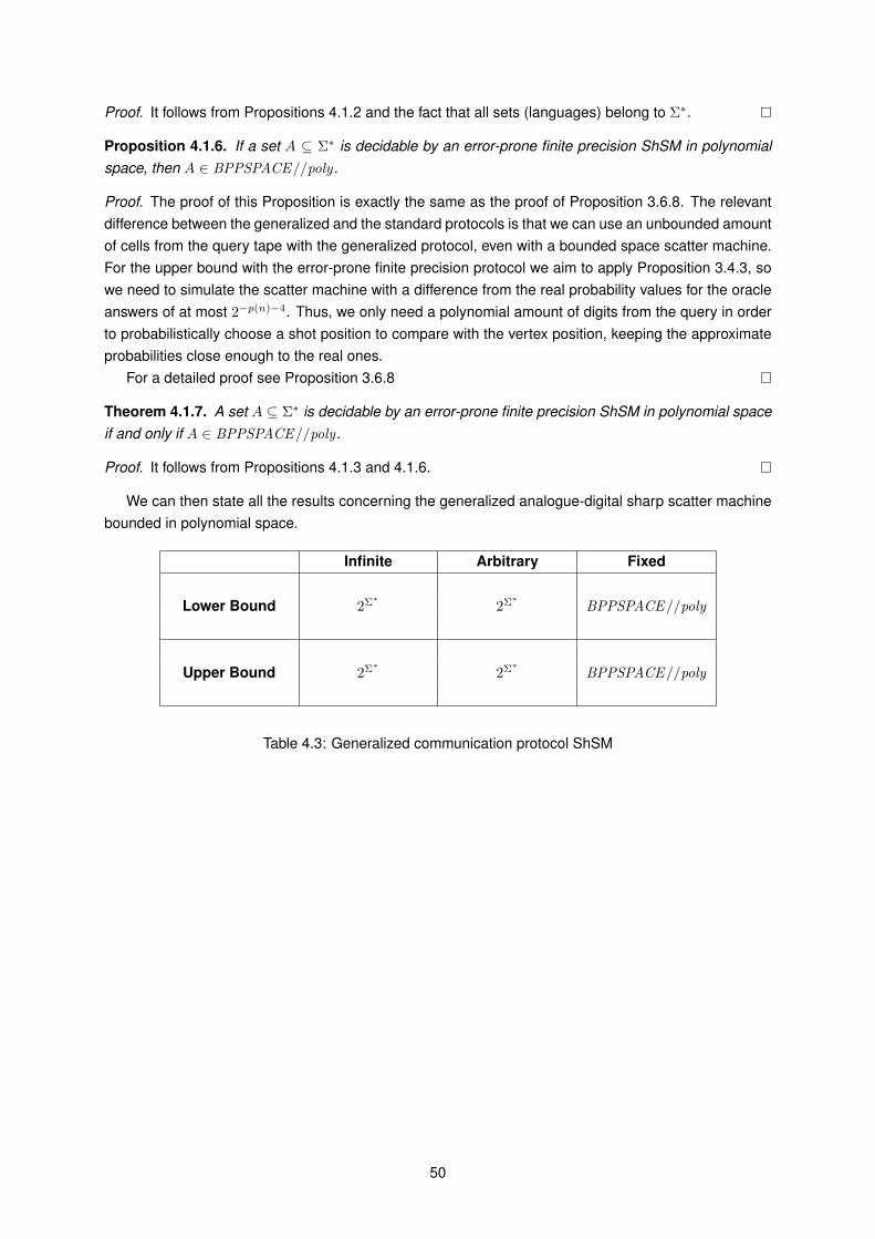
Proof. It follows from Propositions 4.1.2 and the fact that all sets (languages) belong to Σ∗.

Proposition 4.1.6. If a set A ⊆ Σ∗ is decidable by an error-prone finite precision ShSM in polynomialspace, then A ∈ BPPSPACE//poly .

Proof. The proof of this Proposition is exactly the same as the proof of Proposition 3.6.8. The relevantdifference between the generalized and the standard protocols is that we can use an unbounded amountof cells from the query tape with the generalized protocol, even with a bounded space scatter machine.For the upper bound with the error-prone finite precision protocol we aim to apply Proposition 3.4.3, sowe need to simulate the scatter machine with a difference from the real probability values for the oracleanswers of at most 2−p(n)−4. Thus, we only need a polynomial amount of digits from the query in orderto probabilistically choose a shot position to compare with the vertex position, keeping the approximateprobabilities close enough to the real ones.

For a detailed proof see Proposition 3.6.8

Theorem 4.1.7. A set A ⊆ Σ∗ is decidable by an error-prone finite precision ShSM in polynomial spaceif and only if A ∈ BPPSPACE//poly .

Proof. It follows from Propositions 4.1.3 and 4.1.6.

We can then state all the results concerning the generalized analogue-digital sharp scatter machinebounded in polynomial space.

Infinite Arbitrary Fixed

Lower Bound 2Σ∗2Σ∗

BPPSPACE//poly

Upper Bound 2Σ∗2Σ∗

BPPSPACE//poly

Table 4.3: Generalized communication protocol ShSM

50

4.2 Smooth scatter machine

The smooth scatter machine is intrinsically different from the sharp one, in this case we need toguarantee that the experiment do not keeps running indefinitely. To this purpose we may need to usethe time schedule, but we are limited to exponential time schedules since we use scatter machinesbounded in polynomial space (see Proposition 2.1.2). With the fixed precision assumption we can onlyaccess a polynomially long advice, as well as with the sharp scatter experiment, in polynomial space,since we need further space to be able to count the oracle calls needed to obtain a longer advice withthe Chebyshev’s inequality. To the other precision assumptions, if we want to use the time schedule, weare limited to use polynomially long advices as well, since for an exponential time schedule we can onlyuse polynomially sized queries to have the time schedule running in polynomial space on the input size.

Proposition 4.2.1. A set A ∈ Σ∗ is decidable by a generalized smooth scatter machine bounded inpolynomial space, using the time schedule, if and only if is decidable by a standard smooth scattermachine bounded in polynomial space, using the time schedule.

Proof. By Proposition 2.3.1 we have that a set decidable by a standard scatter machine is decidable bya generalized scatter machine.

IfM is a generalized SmSM bounded in polynomial space, using the time schedule, which may usequeries as long as the input, then M can use at most an exponential time schedule (see Proposition2.1.2). The exponential clocks depicted in Section 2.1 use polynomial space on the size of their inputsand thus, used as time schedules the clocks use polynomial space on the size of the queries. Weconclude then that in order to have M running in polynomial space we need to consider queries of atmost polynomial size. IfM only use polynomially sized queries, then a standard SmSM can use exactlythe same queries M uses in any of its computations. Therefore, a standard SmSM can decide all thesets thatM decides, and the desired equivalence follows.

Lower bounds

If we want to use the time schedule, we obtain the same results as with the standard protocol asexplained above. We can decide PSPACE/poly or BPPSPACE//poly with a SmSM with the error-freeprotocol or the error-prone arbitrary precision protocol, respectively (see Propositions 3.7.1 and 3.7.2 fordetailed proofs). If we do not use the time schedule, we can get the same results as in the sharp case,but the scatter machines take, in general, more than exponential time. However, the time the scattermachines take is always guaranteed as finite.

For the lower bounds without time schedule we need the advice function f : N→ Σ∗ detailed for thesharp case lower bound proofs (see Section 4.1).

Proposition 4.2.2. Any set A ⊆ Σ∗ is decidable by an error-free SmSM in polynomial space.

Proof. The proof of this Proposition is, almost in every detail, similar to the proof of Proposition 4.1.1.The remaining difference is that, when using the oracle with the search method of Section 3.1 and thesmooth scatter experiment, the scatter machine takes more than a constant physical time but it can getthe same answers from the oracle and the same computational results. Follows a full proof for the readerseeking the details in this place.

Consider a set A ⊆ Σ∗ lexicographically ordered. Let the advice function f : N → Σ∗ be as de-scribed in Section 4.1 for the the set A, the prefix advice function g : N → Σ∗ be such that g(n) =

f(0)#f(1)# · · ·#f(n) and y ∈ ]0, 1[ be the real number y = 0.x(g) (where x(g) is the encoding x

described in Section 3.1 to the function g). The advice word f(0)#f(1)# · · ·#f(n) is given with two

51

symbols from Σ∗ for each of the symbols 0, 1 or #, so that we have the advice words over Σ∗ and weare able to apply the encoding x to g. We then have that |g(n)| = 2 · (2n+1− 1) + 2n for any n ∈ N, since|f(n)| = 2n.

Consider the error-free SmSM M with vertex position y = 0.x(g) which for an input w with |w| = n

computes the position of w within all the n sized words in Σ∗ ordered lexicographically, lets say that w isthe ith word. Afterwards,M performs 2n+1 − 1 + 2n+ 2i oracle calls with the search method describedin Section 3.1 (which makes the query word into q = x(f(0)#f(1)# · · ·#f(n − 1)#fn1 f

n2 · · · fni )) and

accepts w if and only if the answer from the last call is right, meaning that fni = 1 and so w ∈ A. Weconclude then thatM decides A.

To compute the position of w (|w| = n) within the n sized words in Σ∗ ordered lexicographically, countthe 2n+1 − 1 + 2n + 2i oracle calls and perform them M needs polynomial space on n. So, we canconclude thatM operates in polynomial space (actually in linear space).

The computation time of M on w (|w| = n) is the time needed to compute the position of w andcount the oracle calls plus the time needed to perform the experiments. The time needed to computethe position of w and count the oracle calls is exponential on n. The time needed to perform the 2n+1 −1 + 2n + 2i oracle calls is more than 23·2n+1+6n+6i−4 units of time, since the jth call needs more than23j−1 units of time to be answered. On the other hand, the time needed to perform the 2n+1−1+2n+2i

oracle calls is less than 23·2n+1+6n+6i units of time, since the jth call needs less than 23j+2 units of timeto be answered.

Proposition 4.2.3. Any set A ⊆ Σ∗ is decidable by an error-prone arbitrary precision SmSM in polyno-mial space.

Proof. The proof of this Proposition is, almost in every detail, similar to the proof of Proposition 4.2.2,as well as in the sharp case. The remaining difference is that, when using the oracle with the searchmethod of Section 3.1 and the error-prone arbitrary precision protocol, we need to pad the query wordwith three 0’s in order to get the desired error (accuracy interval) and obtain the same results as with theerror-free scatter machine. Follows a full proof for the reader seeking the details in this place.

Consider a set A ⊆ Σ∗ lexicographically ordered. Let the advice function f : N → Σ∗ be as de-scribed in Section 4.1 for the the set A, the prefix advice function g : N → Σ∗ be such that g(n) =

f(0)#f(1)# · · ·#f(n) and y ∈ ]0, 1[ be the real number y = 0.x(g) (where x(g) is the encoding x

described in Section 3.1 to the function g). The advice word f(0)#f(1)# · · ·#f(n) is given with twosymbols from Σ∗ for each of the symbols 0, 1 or #, so that we have the advice words over Σ∗ and weare able to apply the encoding x to g. We then have that |g(n)| = 2 · (2n+1− 1) + 2n for any n ∈ N, since|f(n)| = 2n.

Consider the error-prone arbitrary precision SmSM M with vertex position y = 0.x(g) which for aninput w with |w| = n computes the position of w within all the n sized words in Σ∗ ordered lexicograph-ically, lets say that w is the ith word. Afterwards, M performs 2n+1 − 1 + 2n + 2i oracle calls with thesearch method described in Section 3.1 (which makes the query word into q = x(f(0)#f(1)# · · ·#f(n−1)#fn1 f

n2 · · · fni )) and accepts w if and only if the answer from the last call is right, meaning that fni = 1

and so w ∈ A. We conclude then thatM decides A.To compute the position of w (|w| = n) within the n sized words in Σ∗ ordered lexicographically, count

the 2n+1 − 1 + 2n + 2i oracle calls and perform them M needs polynomial space on n. So, we canconclude thatM operates in polynomial space (actually in linear space).

The computation time of M on w (|w| = n) is the time needed to compute the position of w andcount the oracle calls plus the time needed to perform the experiments. The time needed to computethe position of w and count the oracle calls is exponential on n. The time needed to perform the 2n+1 −

52

1 + 2n + 2i oracle calls is more than 23·2n+1+6n+6i−4 units of time, since the jth call needs more than23j−1 units of time to be answered. On the other hand, the time needed to perform the 2n+1−1+2n+2i

oracle calls is less than 23·2n+1+6n+6i+1 units of time, since the jth call needs less than 23j+3 units oftime to be answered.

This scatter machine can either take more time than the error-free one from Proposition 4.2.2 or lesstime. The time of each shot can be increased for the double or reduced by a third, the lower boundtime we describe in last paragraph is the same for both Propositions since we took a lower bound whichworks for both cases.

For the fixed precision assumption we are not able to access an exponentially long advice in polyno-mial space by the same reason as in the sharp scatter experiment case. We here state the results, fordetailed proofs see Section 3.7.

Proposition 4.2.4. If a set A ∈ BPPSPACE//poly , then A is decidable by an error-prone finite precisionSmSM in polynomial space, which makes use of the time schedule.

Proof. The proof of this Proposition is exactly the same as the proof of Proposition 3.7.3. The relevantdifference between the generalized and the standard protocols is that we can use an unbounded amountof cells from the query tape with the generalized protocol, even with a bounded space scatter machine.For the lower bound with the error-prone finite precision protocol we do not use this difference since allthe oracle calls with the purpose of obtaining the vertex position are performed with the same query.

For a detailed proof see Proposition 3.7.3

Upper bounds

With the first two precision assumptions (infinite and arbitrary precisions) we get different resultsaccording with if we want the scatter machine to use the time schedule or not. As well as with thestandard communication protocol, in the lower bound proofs, if we want to use the time schedule thismust to be of an exponential growing rate.

Theorem 4.2.5. A set A ⊆ Σ∗ is decidable by an error-free SmSM in polynomial space, using anexponential time schedule, if and only if A ∈ PSPACE/poly .

Proof. It follows from Proposition 4.2.1 and Theorem 3.7.5.

Theorem 4.2.6. The sets decidable by an error-free SmSM in polynomial space, without using the timeschedule, are all the sets A ∈ Σ∗.

Proof. It follows from Proposition 4.2.2 and the fact that all sets (languages) belong to Σ∗.

Theorem 4.2.7. A set A ⊆ Σ∗ is decidable by an error-prone arbitrary precision SmSM in polynomialspace, using an exponential time schedule, if and only if A ∈ BPPSPACE//poly .

Proof. It follows from Proposition 4.2.1 and Theorem 3.7.7.

Theorem 4.2.8. The sets decidable by an error-prone arbitrary precision SmSM in polynomial space,without using the time schedule, are all the sets A ∈ Σ∗.

Proof. It follows from Proposition 4.2.3 and the fact that all sets (languages) belong to Σ∗.

Proposition 4.2.9. If a set A ⊆ Σ∗ is decidable by an error-prone finite precision SmSM in polynomialspace, using the time schedule, then A ∈ BPPSPACE//poly .

53

Proof. The proof of this Proposition is exactly the same as the proof of Proposition 3.7.8. The relevantdifference between the generalized and the standard protocols is that we can use an unbounded amountof cells from the query tape with the generalized protocol, even with a bounded space scatter machine.For the upper bound with the error-prone finite precision protocol we aim to apply Proposition 3.4.5, sowe need to simulate the scatter machine with a deviation from the real probability values for the oracleanswers of at most 2−p(n)−4. Thus, we only need a polynomial amount of digits from the query in orderto probabilistically choose a shot position to compare with the vertex position, keeping the approximateprobabilities close enough to the real ones.

For a detailed proof see Proposition 3.7.8

Theorem 4.2.10. A set A ⊆ Σ∗ is decidable by an error-prone finite precision SmSM in polynomialspace, using the time schedule, if and only if A ∈ BPPSPACE//poly .

Proof. It follows from Propositions 4.2.4 and 4.2.9.

We can then state all the results concerning the generalized analogue-digital smooth scatter machinebounded in polynomial space.

Infinite Arbitrary Fixed

Lower Bound PSPACE/poly BPPSPACE//poly BPPSPACE//poly

with time schedule

Lower Bound 2Σ∗2Σ∗

—without time schedule

Upper Bound 2Σ∗2Σ∗

BPPSPACE//poly

Table 4.4: Generalized communication protocol SmSM

Note that using the time schedule, the upper bounds are also equal to the upper bounds of thestandard case (see Section 3.7). To compute 2Σ∗

with a smooth scatter machine we must be able to useexponential advices, and with that purpose we must use exponentially sized queries. Exponentially sizedqueries take at least 23·2n−1 units of time to be answered (see Proposition 4.2.2) and a time scheduleneeds 3 · 2n − 1 units of space to tick that amount of transitions (see Section 2.1).

54

Chapter 5

Conclusion

With this work we intended to study the computational power of a particular analogue-digital machinebounded in polynomial space, the scatter machine, which consists of a Turing machine coupled with aphysical experiment, the scatter experiment. This computation model was already studied concerningpolynomial time restrictions and we established the results for the polynomial space restrictions.

With an analogue-digital machine of this nature, there are some issues we must discuss concerningits technical behaviour. The scatter experiment has two different versions, the sharp wedge and thesmooth wedge cases. With the smooth wedge we have a physical experiment with intrinsic time costs,and we should deal with it in order to guarantee that no run of infinite time is performed by the experimentin a computation of the analogue-digital machine. Another technical issue is the communication protocolbetween the digital and the analogue components, which must be adapted to the precision that theanalogue component can be set.

Concerning the time issue of the smooth scatter experiment we use a clock to bound the time ofeach run of the experiment. This clock is called time schedule, and as we aim to study scatter machinesbounded in polynomial space we must understand which clocks we can use with that restriction. Thisis a former technique on the subject already used for the time restriction cases, where the clocks to beused must correspond to the general time restrictions. We concluded that in polynomial space we canuse clocks with an exponential growing rate or lower.

Concerning the communication protocols, we studied the three usual different precision assumptions,the infinite precision, the arbitrary precision and the fixed precision. The results to the time restrictionsare established to each one of these precisions with a communication protocol which makes use of adistinguished tape and three or four distinguished states. The Turing machine writes in the query tape theparameters to the experiment, and the conclusions of the experiment lead to the correspondent answerstate. The former communication protocol used for the time restrictions is not sufficient in our case sincethe query tape is restricted by the polynomial space restriction to the machine. We presented a differentcommunication protocol which leads us to different results, and we established the computational resultsfor both protocols.

We concluded that a probabilistic scatter machine with a deterministic digital component is able tosimulate a probabilistic Turing machine with an exponential amount of transitions, using also an expo-nential amount of time. All the usual probabilistic simulations can then be used in this case as they wereused for the time restriction cases.

We use non-uniform complexity classes to describe our results since, as we are using a specific kindof oracle Turing machine, they seem to be appropriate to the purpose. We introduced a probabilisticuniform complexity class, the class of sets decidable by bounded error probabilistic Turing machinesbounded in polynomial space (BPPSPACE ), used then as support for non-uniform classes.

55

We established the computational power for both scatter machines, the sharp and the smooth, andin each case for the two communication protocols, the standard and the generalized. We used adapta-tions of the usual proof techniques, used for the time restriction cases, and another usual technique forwhen the power of the scatter machine allows us to compute all languages. The results for the sharpscatter machine can then be summarized in the following tables, respectively for the standard and thegeneralized protocols.

Infinite Arbitrary Fixed

Lower Bound PSPACE/poly BPPSPACE//poly BPPSPACE//poly

Upper Bound PSPACE/poly BPPSPACE//poly BPPSPACE//poly

Table 5.1: Standard communication protocol ShSM

Infinite Arbitrary Fixed

Lower Bound 2Σ∗2Σ∗

BPPSPACE//poly

Upper Bound 2Σ∗2Σ∗

BPPSPACE//poly

Table 5.2: Generalized communication protocol ShSM

The smooth scatter machine is not that simple to describe as we obtained different results dependingon if we want to use or not the time schedule with the generalized communication protocol. The resultsfor the standard smooth scatter machine can be summarized in the following table.

Infinite Arbitrary Fixed

Lower Bound PSPACE/poly BPPSPACE//poly BPPSPACE//poly

Upper Bound PSPACE/poly BPPSPACE//poly BPPSPACE//poly

Table 5.3: Standard communication protocol SmSM

With the generalized protocol, we obtain the same results as the ones with the standard protocol ifwe use the time schedule, and we obtain the same results as the ones with the sharp scatter machine ifwe do not use the time schedule. All the discussion about the time schedule do not applies to the fixedprecision, since we always need the time schedule in that case, even with the sharp scatter experiment.

56

The results for the generalized smooth scatter machine can be summarized in the following table. Notethat the upper bounds with the generalized protocol are equal to the lower bounds if we want to use thetime schedule, the specified upper bounds are without time schedule.

Infinite Arbitrary Fixed

Lower Bound PSPACE/poly BPPSPACE//poly BPPSPACE//poly

with time schedule

Lower Bound 2Σ∗2Σ∗

—without time schedule

Upper Bound 2Σ∗2Σ∗

BPPSPACE//poly

Table 5.4: Generalized communication protocol SmSM

With this results we can observe that for the fixed precision assumption the results are not differentfrom each other when we change either the communication protocol or the wedge version of the ex-periment. In the protocols case this equality comes from the fact that we always use the same cannonposition to obtain the vertex position, the protocols then make no difference. Concerning the differentversions of the experiment we have the same results as for the time restriction cases, where the compu-tational power is the same with both the sharp and the smooth wedge. This equality comes from the factthat as we use the same cannon position to obtain the vertex position, we use the smooth wedge versionof the experiment with a constant physical time as well as the sharp wedge version, which always has aconstant physical time.

For future work we can suggest, for example, the study of the scatter machine bounded in polynomialspace and clocked in quasi-exponential time (2log(n)k , for some k ∈ N). Here, as we do not bound thetime resource of the general analogue-digital machine, we obtain scatter machines running in exponen-tial time, except when using the generalized smooth scatter machine without the time schedule wherethe time is of the magnitude order of 22n

.For this study it would be useful to use a notation analogous to the one in the conclusion of [7] (§4)

with a new parameter for the space restriction to the machine. This notation could also be useful todescribe the results of our last table as we are, basically, considering different time restrictions with thesame space restriction. The notation describes a complexity class based on the sets computed by theanalogue-digital machines. In our case, with the scatter machine, we could have something like

SCATTER(t(n), s(n), f(n))

where t(n) is the time restriction to the scatter machine, s(n) is the space restriction and f(n) is thebound for the time schedule. We clearly should have f ∈ O(t(n)), otherwise the time restriction wouldnot be followed.

57

References

[1] Tania Ambaram, Edwin Beggs, Jose Felix Costa, Diogo Pocas, and John V. Tucker. Advances inunconventional computing, volume 1 (theory). In Andrew Adamatzky, editor, An analogue-digitalmodel of computation: Turing machines with physical oracles, volume 22 of Emergence, Complexityand Computation, pages 73–115. Springer, 2016.

[2] S. Arora and B. Barak. Computational Complexity: A Modern Approach. Cambridge UniversityPress, 2009.

[3] Jose Luis Balcazar, Josep Dıas, and Joaquim Gabarro. Structural Complexity I. Springer-Verlag,2nd edition, 1988, 1995.

[4] Jose Luis Balcazar and Montserrat Hermo. The structure of logarithmic advice complexity classes.Theoretical Computer Science, 207(1):217–244, 1998.

[5] Edwin Beggs, Pedro Cortez, Jose Felix Costa, and John V. Tucker. Classifying the computationalpower of stochastic physical oracles. page 122, 2016. Submited.

[6] Edwin Beggs, Jose Felix Costa, Bruno Loff, and John V. Tucker. Computational complexity withexperiments as oracles. Proceedings of the Royal Society, Series A (Mathematical, Physical andEngineering Sciences), 464(2098):2777–2801, 2008.

[7] Edwin Beggs, Jose Felix Costa, Bruno Loff, and John V. Tucker. Computational complexity with ex-periments as oracles II. Upper bounds. Proceedings of the Royal Society, Series A (Mathematical,Physical and Engineering Sciences), 465(2105):1453–1465, 2009.

[8] Edwin Beggs, Jose Felix Costa, Diogo Pocas, and John V. Tucker. On the power of thresholdmeasurements as oracles. In Giancarlo Mauri, Alberto Dennunzio, Luca Manzoni, and Antonio E.Porreca, editors, Unconventional Computation and Natural Computation (UCNC 2013), volume7956 of Lecture Notes in Computer Science, pages 6–18. Springer, 2013.

[9] Edwin Beggs, Jose Felix Costa, Diogo Pocas, and John V. Tucker. Computations with oracles thatmeasure vanishing quantities. Mathematical Structures in Computer Science, page 149, 2016.

[10] Edwin Beggs, Jose Felix Costa, Diogo Pocas, and John V. Tucker. An Analogue-Digital Church-Turing Thesis. International Journal of Foundations of Computer Science, 25(4):373–389, 2014. inprint.

[11] Edwin Beggs, Jose Felix Costa, and John V. Tucker. Limits to measurement in experiments gov-erned by algorithms. Mathematical Structures in Computer Science, 20(06):1019–1050, 2010.Special issue on Quantum Algorithms, Editor Salvador Elıas Venegas-Andraca.

[12] Edwin Beggs, Jose Felix Costa, and John V. Tucker. The impact of models of a physical oracle oncomputational power. Mathematical Structures in Computer Science, 22(5):853–879, 2012. Specialissue on Computability of the Physical, Editors Cristian S. Calude and S. Barry Cooper.

58

[13] Edwin Beggs, Jose Felix Costa, and John V. Tucker. Three forms of physical measurement andtheir computability. The Review of Symbolic Logic, 7(4):618–646, 2014.

[14] Edwin Beggs and John V. Tucker. Experimental computation of real numbers by Newtonian ma-chines. Proceedings of the Royal Society, Series A (Mathematical, Physical and Engineering Sci-ences), 463(2082):1541–1561, 2007.

[15] Olivier Bournez and Michel Cosnard. On the computational power of dynamical systems and hybridsystems. Theoretical Computer Science, 168(2):417–459, 1996.

[16] Jose Felix Costa. Turing machines as clocks, rulers and randomizers. Boletim da SociedadePortuguesa de Matematica, 67:121–153, 2012.

[17] Martin Davis. The myth of hypercomputation. In Christof Teuscher, editor, Alan Turing: the life andlegacy of a great thinker, pages 195–212. Springer, 2006.

[18] Martin Davis. Why there is no such discipline as hypercomputation. Applied Mathematics andComputation, 178(1):4–7, 2006.

[19] Kevin T. Kelly. The Logic of Reliable Inquiry. Oxford University Press, 1996.

[20] Hava T. Siegelmann. Computation Beyond the Turing Limit. Science, 268(5210):545–548, April1995.

[21] Hava T. Siegelmann. Neural networks and analog computation : beyond the Turing limit. Birkhauser,1999.

[22] Alan Turing. On computable numbers, with an application to the Entscheidungsproblem. Proceed-ings of the London Mathematical Society, 42:230–265, 1936.

[23] Damien Woods and Thomas J. Naughton. An optical model of computation. Theoretical ComputerScience, 334(2005):227–258, April 2004.

59