sovereign debt, default risk, and the liquidity of government … · in may, 2010, the ecb launched...
TRANSCRIPT

Sovereign Debt, Default Risk, and the Liquidity of
Government Bonds
Gaston Chaumont
Pennsylvania State University
This Version: November 11, 2018�
click here for most recent version
AbstractThe secondary market for sovereign bonds is illiquid and the liquidity is endogenous.Such endogenous liquidity has important e¤ects on the credit spread and the probabil-ity of default. To study equilibrium implications of such liquidity, I integrate directedsearch in the secondary market into a macro model of sovereign default. The model gen-erates liquidity endogenously because investors in the secondary market face a trade-o¤between the transaction costs and the trading probability. This trade-o¤ varies withthe aggregate state of the economy, creating a time-varying liquidity premium over thebusiness cycle. I show that trade �ows in the secondary market signi�cantly a¤ect theprice of sovereign bonds and amplify the e¤ect of default risk on credit spreads. Theimportance of liquidity in the secondary market increases when the economic condi-tions of the issuing country worsen. Illiquidity increases with default risk and accountsfor a sizable fraction of credit spreads, ranging from 10% to 50%.
Keywords: Sovereign Debt; Default; Liquidity; OTC Markets; Directed Search.JEL classi�cation: D83, E32; E43; F34; G12.
�Address: Department of Economics, Pennsylvania State University, 303 Kern Graduate Building, Univer-sity Park, Pennsylvania 16802, USA. I greatly indebted to Shouyong Shi for his continuous advice and encour-agement. I would like to thank Jonathan Eaton, Jingting Fan, Kala Krishna, Rishabh Kirpalani, Kim Rhul,Neil Wallace, Ross Doppelt, Elisa Giannone, Qi Li, Ruilin Zhou, Giang Nguyen, Ignacio Presno, FedericoMandelman, Ed Nosal, Tony Braun, Illenin Kondo, Juan Sanchez, Rody Manuelli, Max Dvorkin, FernandoLeibovici, Fernando Martin, Ana Maria Santacreu, Miguel Faria-e-Castro, Julian Kozlowski, AlessandroDovis and seminar participants at the Graduate Students Conference at WUSTL (2017), Midwest Macro(Fall, 2017, Spring 2018), 7th UdeSA Alumni Conference (2017), Fordham Economics Conference (2018),Atlanta Fed Brown Bag (2018), NASMES (2018), SED (2018), St. Louis Fed Interns Conference (2018), andTrade/Development Reading Group at Penn State for comments and suggestions. In addition, I thank theFederal Reserve Banks of Atlanta and St. Louis for hosting me during the writing of this paper. Finally, Ithank Bates and White fellowship for �nancial support. All errors are of my own.

1 Introduction
A country�s government often issues long-term bonds to sell in the international market.
Before such sovereign bonds mature, they are traded in over-the-counter (OTC) markets.
Trading in this secondary market is decentralized, costly and time consuming.1 The liquidity
of the secondary market a¤ects not only the price of outstanding bonds, but also the price
of new issuances and, hence, the government�s decision on whether to default on the bonds.
In turn, the liquidity of sovereign bonds endogenously depends on the state of the economy
in addition to trading frictions in the secondary market. In this paper, I study sovereign
default incorporating the role of the liquidity of the secondary market, which has been
largely ignored in the sovereign default literature originated in the seminal work of Eaton
and Gersovitz (1981).2 To endogenize the liquidity of bonds, I integrate search frictions in
the secondary market into a general equilibrium model of sovereign debt with default risk.
I use the model to qualitatively and quantitatively study the role of liquidity of bonds on
interest rate spreads and the government�s decision on debt issuance and default. In addition,
the model provides insights on the e¤ects of policy interventions in the secondary markets.
Recent empirical studies have emphasized the role of liquidity on sovereign bond mar-
kets. For example, Beber, Brandt, and Kavajecz (2009) document the e¤ects of liquidity
on sovereign credit spreads over safe bonds, especially during times of heightened market
uncertainty. For the Euro area, Nguyen (2014) reports that, during the 2010-2012 European
debt crisis, even countries with very liquid bonds faced illiquidity periods. She documents
that the relative bid-ask spread - a standard measure of liquidity - of Italian bonds reached
667 basis points,3 an unprecedented level for Italian bonds whose bid-ask spreads are usually
below 50 basis points.4 Large bid-ask spreads were also observed in Ireland and Portugal.
1See, for example, Du¢ e (2012) for details on OTC markets for bonds and World-Bank and IMF (2001)for details structure of sovereign debt markets.
2The only exception in the literature is Passadore and Xu (2018), who impose exogenous trading frictionson individuals selling sovereign bonds in the secondary market.
3The relative bid-ask spread, a standard measure of liquidity, is de�ned as
SB�A � pA � pB12 (p
A + pB)� 10; 000;
where pA is the ask price (the price at which bond dealers sell bonds), pB is the bid price (the price at whichbond dealers buy bonds), and the ratio is multiplied by 10; 000 to measure it in basis points.
4For more details on the importance of liquidity shock in the Eurozone debt crisis, see, for example, Calice,
1

However, the most extreme example is Greece. Bloomberg data shows that bid-ask spreads
for 10 year Greek bonds were about 2; 000 basis points, on average, during the fourth quarter
of 2011, a couple of months before the debt restructuring of March, 2012.
The size of bid-ask spreads during the European debt crisis makes endogenous liquidity
in the secondary market interesting on its own. The policy responses of the European
Central Bank (ECB) and the International Monetary Fund (IMF) make it even more so.
In May, 2010, the ECB launched the Securities Market Programme (SMP) that involved
direct sovereign bond purchases in secondary markets to improve liquidity conditions and
help stabilize distressed sovereign bond yields. As stated by the ECB Press Release of May
10th, 2010, one of the goals of the SMP interventions was "to ensure depth and liquidity
in those market segments which are dysfunctional."5 Bond purchases in secondary markets
do not reduce the debt-to-GDP ratio of the issuing country nor directly improve its �scal
de�cit or aggregate production. How does this type of intervention help overcome a debt
crisis? When are such interventions e¤ective and better than others? The literature does
not provide answers to these questions because it has largely abstracted from endogenous
liquidity.
To model endogenous liquidity, I incorporate frictions in bond markets in the same spirit
as Shi (1995) and Trejos and Wright (1995), for �at money, and Du¢ e, Garleanu, and Ped-
ersen (2005), for corporate bonds. More speci�cally, the model assumes that the sovereign
government sells its debt in a centralized primary market to dealers that act as intermedi-
aries between the government and foreign investors.6 Those dealers then trade bonds with
investors in a decentralized secondary market. In the model, dealers do not have reasons to
hold bonds other than to re-sell them to investors. For their intermediation service, deal-
ers charge investors a transaction fee. On the other side of the market, investors demand
sovereign bonds to maximize expected returns and optimize their portfolio composition. In
Chen, and Williams (2013) and Nguyen (2014). For emerging market bonds, see Hund and Lesmond (2008),who estimate that liquidity frictions are the main source of di¤erences across credit spreads for countrieswithin the same credit rating category.
5See the press release at https://www.ecb.europa.eu/press/pr/date/2010/html/pr100510.en.html. Formore details on the SMP, see Trebesch and Zettelmeyer (2018).
6In reality, only a few large banks can trade in primary bond markets. All other investors, such asindividual investors, institutional investors, and investment funds, need to buy bonds in OTC markets. Inthe model, dealers represent agents of those banks. For the case of Greece, the list of primary dealers canbe found at https://www.bankofgreece.gr/Pages/en/Markets/HDAT/members.aspx.
2

order to be able to trade a bond, investors need to meet dealers in OTC markets, which
are subject to search frictions. An investor�s valuation for a bond incorporates the cost of
intermediation fees, the expected time to trade, and the default risk.
In the secondary market, search is competitive (or directed).7 ;8 In every period, dealers
and investors choose to visit one speci�c submarket in order to search for a trading coun-
terpart. Each submarket is characterized by a transaction fee that the investor needs to
pay to the dealer if they trade. A matching technology determines the number of trades
in each submarket given the numbers of dealers and investors. In equilibrium, investors
and dealers face a trade-o¤ between the intermediation fee and the trading probability. For
an investor, the higher the intermediation fee an investor pays to a dealer, the higher the
investor�s probability of trading. For a dealer, the higher the intermediation fee the dealer
charges, the lower the probability of trading. Facing this trade-o¤, the entry decision of
investors and dealers into submarkets endogenously determine the liquidity of bonds, as well
as transaction fees, the trading volume, and the frequency of trades.
On the qualitative side, the model generates two main new insights. First, trade �ows
between investors and dealers in the secondary market a¤ect the price of newly issued gov-
ernment bonds in the primary market. For example, if the investors��ow of orders in the
secondary market to buy bonds from dealers increases, the demand for bonds by dealers in
the centralized primary market increases. In this case, the bond price must increase to clear
the market and restore equilibrium. Even if the government does not change debt issuances.
Second, there is a positive correlation between default risk and illiquidity in the secondary
market that ampli�es the bonds�interest rates. In equilibrium, the higher the default prob-
ability, the lower the incentives for investors to purchase bonds and the smaller the mass
of investors that show up in the secondary market as buyers. Moreover, as the probability
of default increases, investors holding bonds have higher incentives to �nd a counterpart to
7This modeling is consistent with evidence on the structure of secondary markets. Li and Schurho¤ (2018)analyze dealer networks for US municipal bonds and document that: (i) there is a systematic price dispersionacross dealers, with 20-40% dealer-speci�c variation in markups, (ii) trading costs increase with centralityof the dealer in the network and central dealers charge up to 80% larger spreads, (iii) central dealers placebonds more readily with investors than other dealers, consistent with the notion that they face smaller searchfrictions, and (iv) central dealers provide more liquidity immediacy to investors than peripheral dealers. Thisevidence suggests that investors who desire to trade bonds have a wide range of dealers to visit and thatthey face a trade-o¤ between the markup charged by dealers and the trading probability.
8Well-known examples of directed search models are Peters (1991), Montgomery (1991), Moen (1997),Julien, Kennes, and King (2000), Burdett, Shi, and Wright (2001), and Shi (2001).
3

sell the bonds. Thus, if the sovereign government wants to issue a certain amount of debt
when default probability is high, it will need to induce more dealers to sell bonds in the
secondary market. Because dealers�revenues are transaction fees, these fees must increase in
order to induce more dealers to sell bonds in the secondary market. A higher transaction fee
discourages even more investors from purchasing bonds. As a result, the price of bonds in
the primary market must fall su¢ ciently to induce investors to purchase the desired amount
of newly issued debt. Therefore, the price for bonds in the primary market falls by more
than the amount required to compensate investors for the increased default risk.
I calibrate the model to quantify the e¤ects of liquidity frictions on interest rates. Liquid-
ity frictions signi�cantly contribute to credit spreads. Pricing the pure default probability
and comparing it with total spreads, I �nd that in normal times the model generates credit
spreads that are between 1:5�2 times larger than credit spreads needed to compensate onlyfor default risk. Additionally, credit spreads are more sensitive to negative output shocks.
After a negative output shock, the response in credit spreads at impact is more than 4 times
larger than the response in default risk alone. Thus, liquidity frictions and their interactions
with default risk create a quantitatively important ampli�cation mechanism. Finally, I use
the model to decompose credit spreads in Greece before the debt restructure of 2012.9 I �nd
that between 2006Q1� 2011Q4 the contribution of liquidity frictions to total spreads variesbetween 10%� 50%, reaching 50% right before the Greek debt restructuring.
Related Literature
Sovereign Default. The large body of research on sovereign debt with strategic default
originates in Eaton and Gersovitz (1981), with a strong quantitative focus after the work
by Neumeyer and Perri (2005), Aguiar and Gopinath (2007), and Arellano (2008). Because
debt has long term, my work is closer to Hatchondo and Martinez (2009) and Chatterjee
and Eyigungor (2012)10. I contribute to this literature by endogenizing liquidity in the sec-
9I focus on Greece because it is one of the few countries with a default episode since sovereign bondstrade in OTC markets. Among those countries, Greece is the only country with available data on liquidityof the secondary market.10I abstract from maturity choice decisions. For papers that allow for maturity choice in models with
perfectly liquid sovereign bonds see for example Arellano and Ramanarayanan (2012), Bocola and Dovis(2016), and Sanchez, Sapriza, and Yurdagul (2018). See Kozlowski (2018) for a model of maturity choice inthe context of illiquid corporate bonds.
4

ondary market to study the equilibrium implications for the interest rate spreads and default
probability of sovereign bonds. The framework provides a tool to understand how liquidity
and risk premia interact in equilibrium and how quantitatively important the interaction is
for sovereign bonds�credit spreads, government revenues from new debt issuance, and incen-
tives to default. Furthermore, the framework uses bid-ask spreads and volumes traded in the
secondary market to quantify the importance of liquidity frictions, without compromising
on the tractability of the model. Most papers in the literature on sovereign default have
abstracted from the secondary market completely. Exceptions Broner, Martin, and Ventura
(2010) and Bai and Zhang (2012), incorporate the secondary market into their model, but
they assume the secondary market to be frictionless.11
The most closely related paper is Passadore and Xu (2018), who build on Chen, Cui, He,
and Milbradt (2018) to incorporate trading frictions in the secondary market into a standard
model of sovereign default. Passadore and Xu (2018) impose two assumptions that di¤er
frommine. First, they assume that investors purchase bonds in the primary market, although
investors re-sell bonds in the secondary market. Second, they exogenously �x the probability
of being able to re-sell bonds in the secondary market. Because of these assumptions, their
model is unable to capture how liquidity in the secondary market endogenously responds
to changes in the issuing country�s economic conditions. To capture endogenous liquidity,
I assume that investors both buy and sell bonds in the secondary market and use directed
search to endogenize the trading probabilities in this market.
Endogenous liquidity is important to assess the e¤ects of policy interventions in the
sovereign bond market, such as the securities market programme (SMP) implemented by
the ECB in 2010-2011.12 In my model, interventions of this kind directly a¤ect the price,
the bid-ask spreads, and the liquidity premium of newly issued bonds, by changing the
net demand for bonds in the secondary market. In contrast, if trading probabilities are
exogenous, such interventions may not a¤ect the price of newly issued bonds nor the terms
11This paper also relates to recent papers on the European debt crisis. For example, Bocola and Dovis(2016) study the e¤ects of rollover risk on Italian credit spreads during the crisis, Dovis and Kirpalani (2018)focus on the e¤ects of bailout expectations on interest rate spreads dynamics, and Gutkowski (2018) studiesthe role of sovereign bonds as collateral and the consequences of secondary markets disruptions on output,employment, and investment. I contribute to those papers by incorporating time-varying liquidity frictionsand quantifying their e¤ect on the dynamics of interest rate spreads in Greece.12In section 4.4 I discuss two alternative ways of modeling such interventions and their implications.
5

of trade in bilateral meetings, because the interventions do not a¤ect the outstanding level
of debt or default probabilities.
Asset Liquidity in OTC Markets. This paper is also related to the literature following
Du¢ e et al. (2005) where assets are traded in OTC markets and liquidity is modeled using
search and matching frictions.13 In this literature, there are two type of investors, high and
low valuation investors. In equilibrium, high valuation investors want to purchase debt, while
low valuation investors want to sell because they su¤er from a cost for holding the asset. In
order to trade, investors need to visit a market with search frictions.
In my model, the trading structure in the secondary market is close to Lagos and Ro-
cheteau (2009) and Lester, Rocheteau, and Weill (2015), where (i) trades occur only between
a dealer and an investor but not directly between investors; and, (ii) dealers do not need
to hold inventories as they have permanent access to the centralized primary market that
serves as a clearing system.14 The main contribution of my paper to this literature is to
build a tractable equilibrium model with endogenous liquidity over the business cycle and
strategic default decisions, while this literature usually focuses on steady states and no de-
fault. Another contribution is to endogenize the supply of assets in the secondary market.
The response of this supply to market conditions is critical for understanding endogenous
liquidity, but it is absent in this literature.15
Previous studies also consider endogenous default decisions on corporate bonds. One
example is He and Milbradt (2014). However, the model assumes a stationary environment
where both the characteristics and the supply of assets are �xed over time. Chen et al.
(2018) extend the analysis of He and Milbradt (2014) to allow the aggregate state of the
economy to take two values and show how exogenous reductions in trading probabilities
increase credit spreads. As a result, their model misses two critical features of my model: an
endogenous supply of bonds and endogenous trading probabilities in the secondary market.
They assume that the supply of bonds is �xed over time and that the selling probability is
13This literature derives for monetary theory models of �at money in Shi (1995) and Trejos and Wright(1995).14For a model with market makers (dealers) that accumulate inventories, see Weill (2007).15Exceptions are Geromichalos and Herrenbrueck (2018) where two bond issuers determine the endogenous
supply of competing bonds in a steady state equilibrium and Kozlowski (2018) where companies choose theoptimal size of investment projects and larger projects require larger asset issuance to raise enough funds.However, in both papers the asset supplied is chosen once at t = 0 and kept �xed afterwards.
6

exogenously �xed. As explained above, both features are necessary for understanding how
liquidity of sovereign bonds responds to changes in the state of the economy and a¤ects the
price of new issuance.
Layout. The remainder of the paper is organized as follows. Section 2 describes the en-
vironment of the model economy. Section 3 de�nes an equilibrium of this economy and
characterizes its main theoretical implications. Section 4 illustrates the new channels in the
model. Section 5 calibrates the model and provides quantitative results. Section 6 studies
the Greek debt crisis. Finally, section 7 concludes. The Appendix contains proofs, the solu-
tion algorithm, the description of the data used for the calibration of the model, and some
additional details on the calibration.
2 Environment
Time is discrete and in�nite. There are three types of agents: (i) a sovereign government;
(ii) dealers; and (iii) foreign investors.
The country of interest faces a random endowment process yt 2 �Y � [ymin; ymax], whichis Markovian. The government maximizes the lifetime value of the representative household
in the country, given by1Xt=0
�tU (ct) ;
where U (�) is strictly increasing and concave, ct is household�s consumption, and � 2 (0; 1)is the discount factor. The government can save or borrow from international credit markets,
described later in this section.
At the beginning of each period the outstanding debt is Bt. The government chooses
whether to default or not on its outstanding debt obligations. If the government defaults on
the debt, there are two costs. The �rst cost is a temporary exclusion from �nancial markets
that prevents the government from borrowing or saving while in �nancial autarky. While
the government is in default, every period it can re-gain access to �nancial markets with
exogenous probability � 2 (0; 1).16 Upon re-gaining access to credit markets, the government
16For models with endogenous market re-access see Yue (2010) and Benjamin and Wright (2013).
7

starts with no outstanding debt. The second cost is an output cost, i.e., under default the
endowment is given by h (yt) = yt (1� ! (yt)), where ! (yt) is a (weakly) increasing functionof yt.
If the country does not default on debt, the country is in good credit conditions. In this
case the government can save or issue debt, Bt+1 2 �B � [Bmin; Bmax], in the primary bondmarket (B > 0 means debt while B < 0 means credit). When the government issues debt,
the bonds are sold to dealers in the primary market, which is Walrasian.17 The sovereign
government takes as given the price schedule of bonds p (yt; Bt;t; Bt+1), which is determined
in equilibrium. The arguments of this pricing schedule are the current level of endowment,
which allows investors to forecast next period�s endowment, the current level of debt, Bt,
the current distribution of investors with respect to their types and asset holdings, t, and
Bt+1.
The maturity of bonds is determined by a parameter �. As it is usually assumed in the
literature, each unit of debt matures with probability � 2 [0; 1] in every period, independentlyof when that unit of debt was issued (e.g., Hatchondo and Martinez (2009)). Thus, the
average time to maturity of each bond is 1�periods. Each unit of unmatured bond pays
a coupon z � 0 every period. Therefore, the period t budget constraint of the sovereign
government that is in good credit conditions is given by
ct + [�+ (1� �) z]Bt � yt + p (yt; Bt;t; Bt+1) [Bt+1 � (1� �)Bt] :
The left hand side represent expenditures on consumption, coupon payments, and repayment
of matured bonds. The right hand side represents incomes from endowment and new debt
issuances.
Dealers are risk-neutral. They can access the primary market without cost and purchase
bonds issued by the government at the competitive price, p (yt; Bt;t; Bt+1). That is, there
are no frictions in the primary market. Also, it is assumed that dealers have permanent
access to this primary market so that they only purchase bonds when they want to sell it to
an investor. This simpli�cation avoids working with dealers that hold inventories of the bond.
17The government could organize an auction to sell the bonds. Since in this model there is complete andperfect information about valuations of the bonds, the auction could be designed to extract all the surplusfrom dealers. That is, dealers would be acting as if there is perfect competition among them.
8

In addition, dealers have access to a frictional secondary market where they can trade with
foreign investors. This secondary market is characterized by directed search. Speci�cally,
there is a continuum of submarkets that are characterized by the transaction fee that dealers
charge to investors in case a trade occurs. Entry into submarkets is competitive. To enter
any submarket, a dealer needs to pay a per-period �ow cost, .18 A dealer compensates the
entry cost by the bid-ask spread between submarkets. As the only intermediators between
the primary and the secondary market, dealers collect the orders from the secondary market
and clear the net demand (or supply) in the primary market at the end of each period.
Investors in the secondary market are from foreign countries with a �xed measure �I �Bmax. They can trade bonds only by meeting a dealer. In order to trade, investors choose the
submarket to enter. That is, investor�s search for dealers is also directed. For simplicity, I
assume that investors can only hold either zero or one unit of the bond. I denote an investor�s
bond holdings a 2 f0; 1g. There are two types of investors, denoted ` and h. Type i 2 f`; hginvestors have preferences ui over the bond, with uh > u`, in addition to other consumption
c. These di¤erent preferences will generate gains from trade for investors in equilibrium.
Investors enter the economy as type h and without bonds. In equilibrium these investors
will be the ones willing to purchase sovereign debt. Once a type h investor acquires a unit
of the bond, the investor starts to face a preference shock with probability � 2 (0; 1), whichchanges the investor into type `. In the equilibrium, type ` investors are the ones willing
to sell the bonds in the secondary market. For simplicity, I assume that once an investor
that gets rid of the bond, the investor leaves the economy and is replaced by a new type h
investor who does not have the bond. There are two ways that an investor can get rid the
bond: (i) by selling it to a dealer in the secondary market, or (ii) by waiting for the bond
to mature, which occurs every period with probability �. Finally, investors have access to a
risk-free, perfectly liquid, one period zero-coupon bond that pays an exogenous return r > 0.
In each submarket in the secondary market, there is a constant returns to scale order
processing technology denoted M (d; n), where d is the number of dealers in a submarket
and n is the number of investors. Each order is equally likely to be executed at any time.
The probability of an order being executed is given by � (�) � M(d;n)n
= M (�; 1), with
18This cost can be interpreted as a constant marginal cost of allocating a dealer into a submarket, for abank that participates in the primary market.
9

� � dn. The amount of orders executed by a dealer in a period of time is then � (�) � M(d;n)
d.
I assume that M (�; �) is such that � (0) = 0, � (1) = 1, � (1) = 0, and � (�) is strictlyincreasing and concave.
Within each period, the timing of actions within a period is as follows:
1. Shock y is observed. The government decides whether or not to default. If the gov-
ernment defaults the bond is not available as a possible investment choice for investors
anymore, and investor�s and dealer�s problems are irrelevant.
2. If the government repays, then the government chooses issuances, B0, optimally.
3. A fraction � of B matures. Their owners are replaced by h investors without bonds.
Principal of matured bonds is paid to current bond owners. Unmatured bonds pay
coupon, z, and yield utility ui to investors of type i 2 f`; hg.
4. Investors�preference shock is realized and a fraction � of type h investors with a unit
of a bond become type ` investors.
5. The centralized primary market and the decentralized secondary markets open. In the
centralized primary market, the government and dealers trade at a competitive price.
Investors and dealers decide optimally which submarket to visit and, those who meet
a counterpart, trade in the secondary market.
Notice that by the time investors make their submarket choice decisions in step 5, govern-
ment�s debt issuance B0 is already known. Thus, if the government is under good credit con-
ditions, the relevant state of the economy for investors is given by st = (yt; Bt;t; Bt+1) 2 S,where S represents the space of all possible values for st. That is, the current aggregate state
of the economy consists of the current level of output, yt, the outstanding level of debt at
the beginning of period t, Bt, the distribution of investors�types and bond holdings at the
beginning of period t, t, and government�s choice of next period�s level of debt, Bt+1.
In the following subsections I formulate the government�s, investors�, and dealers�prob-
lems.
10

2.1 Government
At the beginning of each period, the government chooses whether to default, � = 1, or repay,
� = 0, and the optimal debt issuance in case of repayment. The government�s value function
is:
V (y;B;) = max�2f0;1g
�(1� �)V R (y;B;) + �V D (y)
, (1)
where V R (�) is the value of repaying debt obligations and V D (�) is the value of default. Thevalues come from domestic households�intertemporal utility. The value of default is given
by
V D (y) = U (h (y)) + �Ey0jy��V (y0; 0;0) + (1� �)V D (y0)
�: (2)
That is, if the government decides to default, it does not need to repay outstanding debt
so it will consume the total output of the current period. However, there is an output cost
associated to the default decision so today�s consumption is given by the function h (y) =
yt (1� ! (yt)). In addition, the continuation value is a weighted sum of the value of re-gainingcredit access, which happens with probability �, and starting next period in default, which
happens with probability (1� �). Notice that if the government re-gains access to credit,it starts with zero outstanding debt and investors distribution 0, with all investors being
high type with no bond holdings. In the case of not defaulting the debt, the government
chooses consumption of the domestic household, c, and the new stock of debt, B0. The value
of repaying debt is given by
V R (y;B;) = maxc;B0
�U (c) + �Ey0jyV (y0; B0;0)
, s:t: :
[BCG] : c+ [�+ (1� �) z]B = y + p (y;B;; B0) [B0 � (1� �)B] .
z is the coupon paid to the bond. The price schedule p (y;B;; B0) is determined endoge-
nously in the primary debt market and depends on the amount of new debt issued by the
government. The government internalizes how the price of debt issuances changes as it
changes the level of debt issued for next period but it takes as given this pricing function.
11

Using the constraint to substitute c, the objective function becomes:
V R (y;B;) = maxB0fU (y + p (y;B;; B0) [B0 � (1� �)B]� [�+ (1� �) z]B) (3)
+�Ey0jyV (y0; B0;0)g:
2.2 Foreign Investors
Foreign investors trade the bond in the secondary market. To describe an investor�s decision,
I denote the set of submarkets as �F = [fmin; fmax] which is a compact space. To de�ne this
space, let fmin � since no dealer will be willing to enter a submarket that does not pay
enough to cover the entry cost. In addition, the price for a bond that matures with probability
�, with a �ow return (z + uh) every period until maturity, and that never defaults would be�+(1��)(z+uh)
�+r. Thus, we can de�ne fmax � �+(1��)(z+uh)
�+rsince no investor would be willing to
pay a higher intermediation fee, even if the trading probability is equal to one.
Denote the value functions of a type i investor holding a unit of the bond as Iai , where
i 2 f`; hg and a 2 f0; 1g. Note that the combination i = ` and a = 0 never occurs because,after getting rid of the bond, the investor leaves the economy and is replaced by a new type
h investor with a = 0. I formulate the decision problem for an investor below.
2.2.1 High Type Investors without a Bond
For each state s = (y;B;; B0) 2 S, the value for a type h investor with a = 0 is given by
I0h (s) = maxff� (� (f))
��p (s)� f + 1
1 + rEy0jy [1� � (y0; B0; L01)] I1h (s0)
�(4)
+1� � (� (f))
1 + rEy0jy [1� � (y0; B0; L01)] I0h (s0)g:
The investor chooses optimally which submarket to visit (how much transaction fee, f , he
wants to pay) in order to purchase a unit of the sovereign bond. In submarket f , the investor
will be able to trade with a dealer with probability � (� (f)). Once matched, the investor
purchases a unit of the bond after paying its price in the primary market, p (s), plus the
transaction fee, f . In addition, holding a bond derives a continuation value of being a type
h investor in the next period, I1h (s0), provided that the government does not default on the
12

bond when next period starts. The continuation value is discounted at the rate r, which is
the rate of return on the perfectly liquid, risk-free bond. If the investor is not matched with
a dealer, which happens with probability 1 � � (� (f)), the investor receives the discountedcontinuation value of being type h with a = 0 at the beginning of the next period, conditional
on the government not defaulting on the bond. If the government defaults on the bond, the
continuation value of holding the bond is zero.
2.2.2 High Type Investors with a Bond
The value function for a type h investor with a = 1 is as follows,
I1h (s) = �+ (1� �) (uh + z) + ��I1` (s)� �� (1� �) (u` + z)
�(5)
+(1� �) (1� �)maxff� (� (f)) [p (s)� f ]
+[1� � (� (f))]
1 + rEy0jy [1� � (y0; B0; L01)] I1h (s0)g:
The investor obtains the face value, 1, if the bond matures, which occurs with probability �.
If the bond does not mature, the investor enjoys utility uh from holding it and the coupon
payment z. In addition, the investor is hit by the preference shock with probability �, which
changes the investor to a type ` investor with a = 1. The payo¤ in this case is described
below. The other terms multiplied by � inside the squared bracket are there to avoid double
counting �ows of payments and utility of the bond (see equation 7 below). If the investor
is not hit by the preference shock and the bond does not mature, the investor might be
matched to a dealer in submarket f or not. In the case of a match the investor sells the
bond and receives the price of the bond p (s) minus the transaction fee, f , paid to the dealer.
If the investor is not matched with a dealer there is no trade and the investor receives the
discounted continuation value of being type h with a = 1 at the beginning of next period,
conditional on the government not defaulting on the bond. If the government defaults on
the bond, the continuation value is zero.
For a type h investor with a = 1 to chose to enter a submarket f > 0, the price p (s)
should be very attractive as these investors like holding the bond. The following condition
13
is necessary and su¢ cient for this to happen:
f > 0 () p (s) >1
1 + rEy0jy [1� � (y0; B0; L01)] I1h (s0) : (6)
Notice that, since I0h (s0) � 0 and the bene�t of purchasing the bond for the type h investors
with a = 0 is given by
1
1 + rEy0jy [1� � (y0; B0; L01)]
�I1h (s
0)� I0h (s0)�;
then, whenever (6) holds no investor is willing to purchase a bond. Thus, only investors
trying to sell will show up in secondary markets, which can only occur in the case that the
sovereign government decides to retire a large amount of bonds from the market. Therefore,
re-purchasing bonds is expensive for the government because it needs to pay a price higher
than the valuation of type h investors.
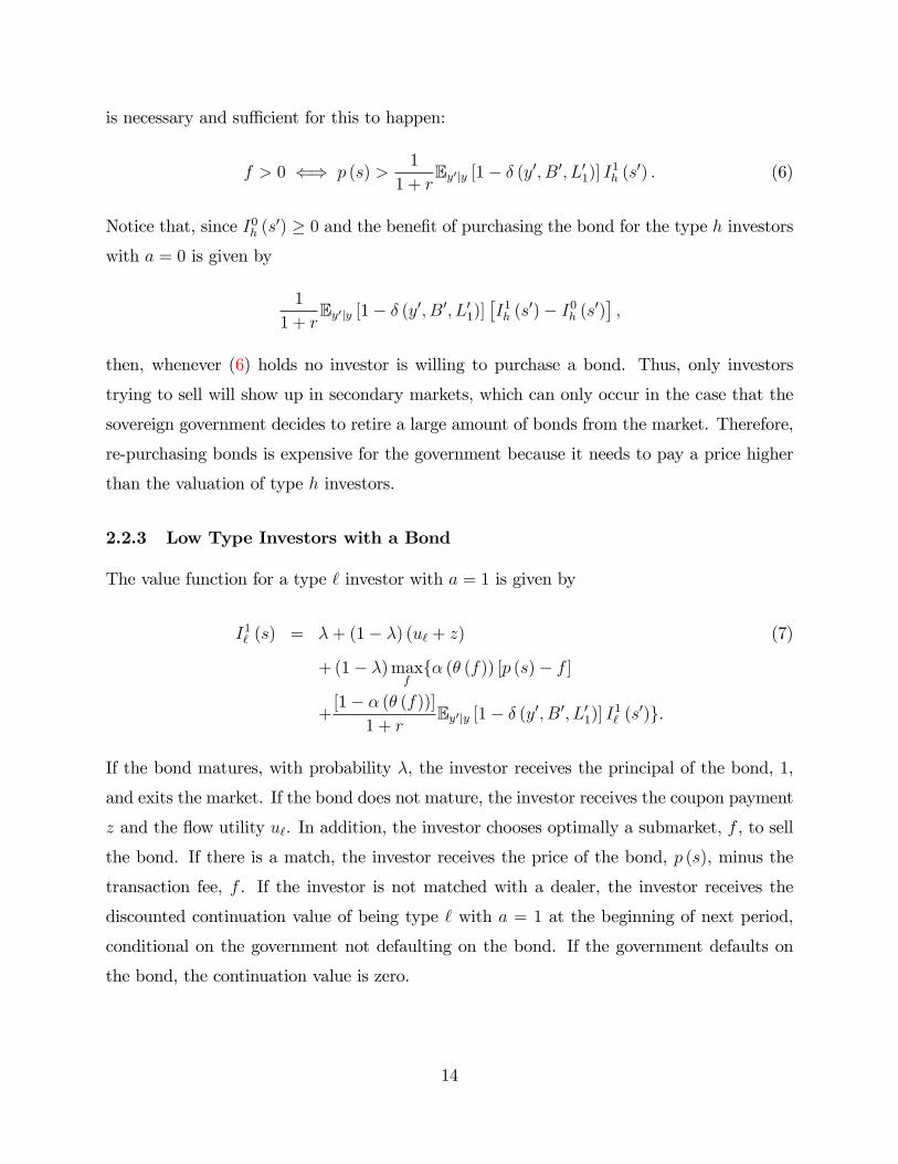
2.2.3 Low Type Investors with a Bond
The value function for a type ` investor with a = 1 is given by
I1` (s) = �+ (1� �) (u` + z) (7)
+(1� �)maxff� (� (f)) [p (s)� f ]
+[1� � (� (f))]
1 + rEy0jy [1� � (y0; B0; L01)] I1` (s0)g:
If the bond matures, with probability �, the investor receives the principal of the bond, 1,
and exits the market. If the bond does not mature, the investor receives the coupon payment
z and the �ow utility u`. In addition, the investor chooses optimally a submarket, f , to sell
the bond. If there is a match, the investor receives the price of the bond, p (s), minus the
transaction fee, f . If the investor is not matched with a dealer, the investor receives the
discounted continuation value of being type ` with a = 1 at the beginning of next period,
conditional on the government not defaulting on the bond. If the government defaults on
the bond, the continuation value is zero.
14

2.3 Dealers
Dealers participate competitively in debt markets. Each dealer chooses an intermediation
fee to be charged to investors for intermediation services. To enter any given submarket a
dealer needs to pay a �ow cost > 0. A dealer posts the intermediation fee to maximize
expected pro�ts:
� = maxf �2F
f� (� (f)) f � g; (8)
where � (�) represents the probability of being able to execute an order, derived from the
order execution technologyM described earlier. Competitive entry of dealers implies that
the following condition of complementary slackness
�(f) � 0 and � (f) � 0. (9)
Whenever expected pro�ts for dealers are negative in a submarket f , the market tightness
� (f) in this submarket is zero since no dealers have incentives to participate in this sub-
market. On the other hand, whenever the market tightness is positive, a positive mass of
dealers participate of the submarket, in which case expected pro�ts for each dealer should
equal zero.
Condition (9) provides a mapping from each submarket intermediation fee, f , to the
tightness in that submarket. This mapping is given by
� (f) =
8<: ��1� f
�if �(f) = 0,
0 otherwise.: (10)
2.4 Market Clearing
The primary market is Walrasian and only government and dealers can access it. In each
state s 2 S and conditional on the government being in good credit standards, the pricep (s) must clear the bonds primary market.
Recall that �I is the total mass of investors. Let H0 be the mass of type h investors with
a = 0, H1 the mass of type h investors with a = 1, and L1 the mass of type ` investors
with a = 1. All of these are measured at the beginning of a period. At the beginning of
any given period, �I = H0 + H1 + L1. In addition, all outstanding bonds must be held by
15

some investors. That is, B = H1 +L1. Using this notation, the total supply of bonds in the
primary market is given by
max fB0; 0g � (1� �)B| {z }Government�s supply
+ ���1`�� (1� �)H1| {z }
New sellers�supply
+���1`�(1� �)L1| {z }
Old sellers�supply
+ ���1h�(1� �) (1� �)H1| {z }
Potential type h sellers
:
The �rst term is the government�s new bond issuances. The operator max fB0; 0g capturesthe possibility that the government chooses B0 < 0, in which case the government can at
most demand the (1� �)B outstanding bonds in the primary market. The second term is
the supply of bonds from "new sellers", i.e., type h investors who are hit by the preference
shock (� of them) to become type ` investors. They sell their bond holdings. Since a fraction
� of them will see their bond mature, only 1 � � will be trying to sell the bond. Amongthe sellers, only a fraction �
��1`�will get matched with a dealer. �1` is the tightness in the
submarket optimally chosen by type ` investors. The third term above is the supply of bonds
by "old sellers." Similarly to the second term, it consists of those type ` investors that are
holding a bond who were not able to sell it in the past, for which the bond did not mature,
and who got matched with a dealer. Finally, the fourth term is the potential supply of bonds
by type h investors with a = 1, which is positive if and only if condition (6) holds.
On the other side of the primary market, the demand for bonds, are the buying orders
received by dealers from the fraction of type h investors, ���0h�:
���0h�H0| {z }
Old Buyers�demand
+ ���0h��B| {z }
New Buyers�demand
.
The �rst term represents "old buyers," i.e. type h investors with a = 0 who are in the
market from the last period. The second term, represents the "new buyers," i.e. those type
h investors who entered the economy in the current period to replace the investors that left
the economy after their unit of the bond matured. The tightness �0h corresponds to the
submarket optimally chosen by type h investors with a = 0.
The distribution of investors types and bond holdings is , which consist of the three
measures fH0; H1; L1g. However, since H1 = B � L1, and since all type ` investors visit the
16

same submarket independently of their type in the previous period, the total supply from
investors trying to sell their unit of the bond can be written as
���1`�(1� �) [�B + (1� �)L1] .
In addition, �I = H0 + H1 + L1 = H0 + B, and so H0 = �I � B. Hence, I de�ne the excessdemand function for each state s 2 S as
ED (s) � ���0h (s)
� �I � (1� �)B
�| {z }Buyers�demand
� [max fB0; 0g � (1� �)B]| {z }Government�s supply
����1` (s)
�(1� �) [�B + (1� �)L1]| {z }Sellers�supply
� ���1h (s)
�(1� �) (1� �) (B � L1)| {z }
Potential type h sellers
:
Now, the only element of in this excess demand function is L1. Therefore, we only need
to keep track of L1 instead of as the aggregate state variable describing the distribution
of investor types and bond holdings. As I will show later, this excess demand function is
consistent with only one price p (s) clearing the market, for each state s.
Finally, the law of motion for the aggregate state variable L1 is given by
L01 = (1� �)�1� �
��1`��L1 + � (1� �)
�1� �
��1`��H1 (11)
= (1� �)�1� �
��1`��[(1� �)L1 + �B] :
There is no uncertainty about the future value L01 since it is completely determined by the
current state and the tightness, �1` , at the optimally chosen submarket f1` .
3 Equilibrium
I �rst de�ne an equilibrium for this economy in section 3.1 and then proceed to characterize
the properties of the equilibrium in section 3.2.
3.1 Equilibrium De�nition
The equilibrium concept used here is recursive competitive equilibrium.
17

De�nition 1 A Recursive Competitive Equilibrium (RCE) in this economy consists of a set
of value functions�V; V R; V D; I0h; I
1h; I
1` ;�
, a set of policy functions f�; B0; f0h ; f1h ; f1` g, a
tightness function �, and a pricing function p, such that for all s = (y;B; L1; B0) 2 S:
1. Given functions p (s), f 1` (s), � (s), the functions V (y;B; L1), VR (y;B; L1), V D (y),
� (y;B; L1), B0 (y;B; L1), solve the sovereign government�s problem in (1)-(3);
2. Given p (s), � (y;B; L1), B0 (y;B; L1), � (s), the functions I0h (s), I1h (s), I
1` (s), f
0h (s),
f 1h (s), f1` (s) solve the investor�s problem in (4), (5), and (7);
3. The tightness function � (s) is consistent with free entry of dealers and determined by
(10);
4. The function p (s) clears the primary market of bonds; and
5. The expected law of motion for the aggregate state L1 is consistent with policy functions
and given by (11).
3.2 Equilibrium Characterization
3.2.1 Government�s Problem
Government�s problem de�ned by equations (1)� (3), looks exactly like a standard sovereigndefault model. The new channels arising due to liquidity frictions in secondary markets
only enter into the problem through the budget constraint in the value of repaying debt,
V R (y;B; L1), in (3). In particular, liquidity friction a¤ect the price schedule for new bond
issuances, p (y;B; L1; B0), through the state variable L1, which measure the mass of low
type investors at the beginning of current period. However, for any given price schedule
the government problem satis�es standard properties in the literature. In Appendix A.1, I
repeat some of the standard arguments to characterize the solution of government�s problem
for a given price schedule, p (s). Later, I will examine the existence of the price schedule in
equilibrium and how it is a¤ected by liquidity frictions.
18
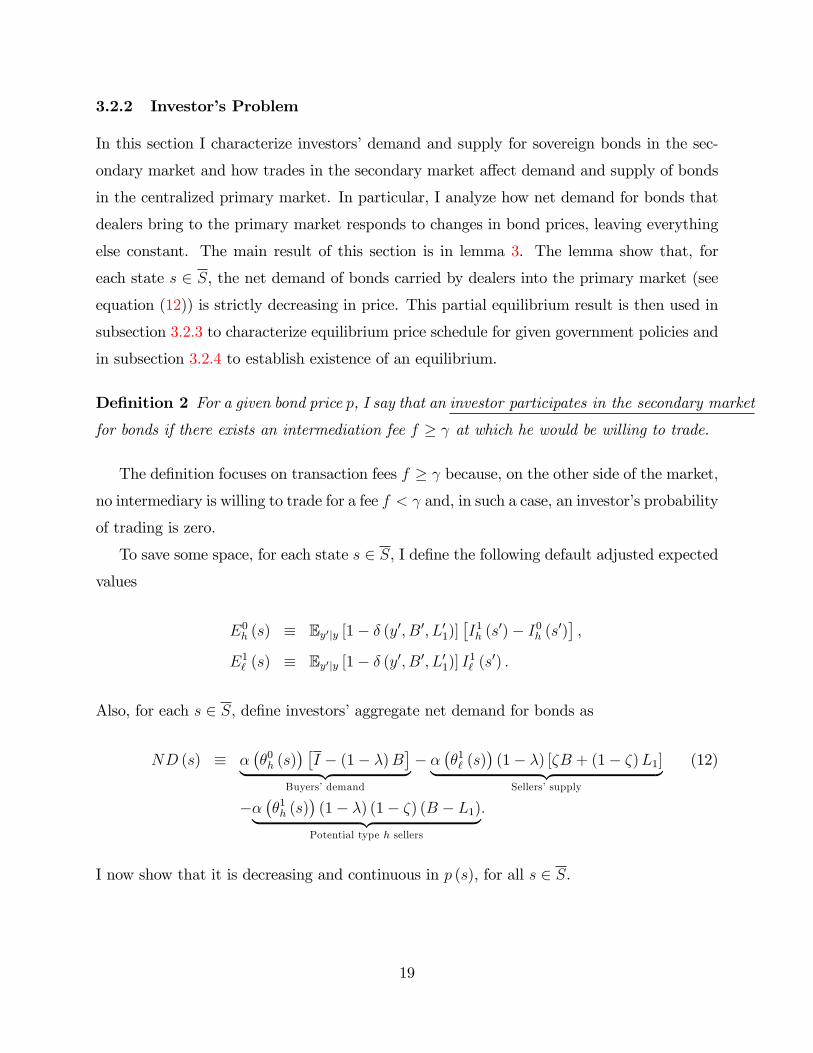
3.2.2 Investor�s Problem
In this section I characterize investors�demand and supply for sovereign bonds in the sec-
ondary market and how trades in the secondary market a¤ect demand and supply of bonds
in the centralized primary market. In particular, I analyze how net demand for bonds that
dealers bring to the primary market responds to changes in bond prices, leaving everything
else constant. The main result of this section is in lemma 3. The lemma show that, for
each state s 2 S, the net demand of bonds carried by dealers into the primary market (seeequation (12)) is strictly decreasing in price. This partial equilibrium result is then used in
subsection 3.2.3 to characterize equilibrium price schedule for given government policies and
in subsection 3.2.4 to establish existence of an equilibrium.
De�nition 2 For a given bond price p, I say that an investor participates in the secondary market
for bonds if there exists an intermediation fee f � at which he would be willing to trade.
The de�nition focuses on transaction fees f � because, on the other side of the market,no intermediary is willing to trade for a fee f < and, in such a case, an investor�s probability
of trading is zero.
To save some space, for each state s 2 S, I de�ne the following default adjusted expectedvalues
E0h (s) � Ey0jy [1� � (y0; B0; L01)]�I1h (s
0)� I0h (s0)�;
E1` (s) � Ey0jy [1� � (y0; B0; L01)] I1` (s0) :
Also, for each s 2 S, de�ne investors�aggregate net demand for bonds as
ND (s) � ���0h (s)
� �I � (1� �)B
�| {z }Buyers�demand
� ���1` (s)
�(1� �) [�B + (1� �)L1]| {z }Sellers�supply
(12)
����1h (s)
�(1� �) (1� �) (B � L1)| {z }
Potential type h sellers
:
I now show that it is decreasing and continuous in p (s), for all s 2 S.
19

Lemma 3 For any s 2 S, and given a government�s default policy function � (y;B; L1),
investors�aggregate net demand de�ned in (12) is continuous and decreasing in p (s). More-
over, if1
1 + rE1` (s) + <
1
1 + rE0h (s)� ;
it is strictly decreasing for all p (s) 2 R+, and if
~p2 (s) �1
1 + rE1` (s) + �
1
1 + rE0h (s)� � ~p1 (s) ;
it is constant for all p (s) 2 [~p1 (s) ; ~p2 (s)] and strictly decreasing for all p (s) in the comple-ment of this set in R+.
Proof. See Appendix A.2.
I provide the details of the proof as well as necessary intermediate results in Appendix
A.2. The result in lemma 3 is intuitive. It states that given a government�s default policy
function the dealers�net demand for bonds in the primary market is decreasing in the price
of the bond, and strictly decreasing in most of the cases. This follows because the mass of
type h investors with a = 0 buying from dealers is decreasing in the price of the bond and
the mass of investors holding a bond that sell bonds to dealers is increasing in the price of
the bond. The mass of type h investors with a = 0 that meet dealers is decreasing in p
because the dealer charges the investor p+f 0h (s), and so the investor pays more for the same
expected return. Therefore, the investor responds by optimally reducing the intermediation
fee f 0h (s). As a result, dealers earn lower expected pro�ts and there is less entry into the
secondary market, which in turn reduces the matching probability of investors trying to
purchase bonds. As the each investor�s trading probability decreases, a smaller mass of
them trade. An opposite argument explains why the mass of investors selling their bonds to
dealers increases with p.
3.2.3 Bond Market Clearing Prices
I now use the results in section 3.2.2 to show that for each state s 2 S and given a govern-ment�s default policy function � (y;B; L1), there is a unique price that is consistent with mar-
ket clearing. Then, I characterize the pricing schedule faced by the government. Throughout
20

this subsection I denote B (s), L1 (s), and B0 (s) the second, third, and fourth component of
s = (y;B; L1; B0), respectively.
For each s 2 S and any given price p, de�ne the excess demand function for bonds in theprimary market as
ED (s; p) � ND (s; p)� [B0 (s)� (1� �)B (s)] ; (13)
with ND (s; p) de�ned as in (12).
Proposition 4 If1
1 + rE1` (s) + <
1
1 + rE0h (s)� ;
for any policy function � (y;B; L1) and any s 2 S such that B0 (s) > 0, there is a unique
price p (s) 2 R+ consistent with
p (s)ED (s; p (s)) = 0. (14)
Moreover, either p (s) > 0 and ED (s; p (s)) = 0, or p (s) = 0 and ED (s; p (s)) � 0. In
addition, when
~p2 (s) �1
1 + rE1` (s) + �
1
1 + rE0h (s)� � ~p1 (s) ;
the result still holds except when B0 (s) = (1� �)B (s), in which case any price within[~p1 (s) ; ~p2 (s)], is consistent with p (s)ED (s; p (s)) = 0.
Proof. See Appendix A.3.
Given this result, we can then characterize the price schedule faced by a government
conditional on a given policy function � (y;B; L1).
Corollary 5 The price schedule faced by a government conditional on a given policy function
� (y;B; L1) is given by
p (s) =
8<: fx 2 R+ : ED (s;x) = 0g if ND (s; 0) > B0 (s)� (1� �)B (s)0 if ND (s; 0) � B0 (s)� (1� �)B (s)
: (15)
Proof. Directly follows from the previous results.
21

The price schedule de�ned in (15) replaces the standard no-arbitrage condition usually
found in the literature of sovereign default. Proposition 4 states that the price that clears the
primary market for sovereign bonds is unique, except for a particular cases in which neither
the government nor the dealers participate in the primary market. To be more precise,
this uniqueness statement is conditional on given a government�s default policy function,
investors value functions, and future expected prices. However, the result highlights the
parallelism of the pricing schedule to the standard no-arbitrage condition that maps future
prices and a default policy function into current prices. In this sense, solving this model
is not harder than a standard model of sovereign default. Instead of having a closed form
expression for the price as in standard no arbitrage condition, I just need to �nd the price
consistent with (14).
3.2.4 Equilibrium Existence
In this section I show existence of an equilibrium for the economy outlined in section 2.
Proposition 6 An equilibrium exists.
Proof. See Appendix A.4.
The arguments of the existence proof follow standard arguments in the literature making
use of the Kakutani-Fan-Glicksberg �xed point theorem (see Aliprantis and Border (2006)
theorem 17.55). The new important part of the argument is replacing the standard no arbi-
trage condition by the market clearing price in the centralized primary market characterized
by the mapping in (15). Using the results in section 3.2.3 I can show that the new mapping
for the pricing schedule satis�es all required conditions and standard arguments can be ap-
plied to the model described in section 2. The details of the proof are provided in Appendix
A.4.
22

4 Main Mechanisms and the Role of Liquidity
4.1 An Illustrative Example
To build intuition, I consider a particular case in which I can write a closed form expression
for the pricing schedule de�ned in (15).19 In particular, I assume that the order processing
technology (matching function) is Cobb-Douglas and given by
M (d; n) = �0d1=2n1=2:
In addition, I assume that high type investors never become low type, � = 0, and uh = u` = 0.
If no investor becomes low type, the measures of investors at the beginning of each period
are
H0 =�I � (1� �)B
�; H1 � (1� �)B; L1 � 0:
Under these assumptions, it is easy to solve for the price schedule. Whenever the government
is issuing new debt, I can write the price in the primary market as
p (s) =1
1 + rEy0jyf
�I1h (s
0)� I0h (s0)�
| {z }Value of holding bond
[1� � (y0; B0; 0)]| {z }Default Risk
g � 2 �20
B0 � (1� �)BI � (1� �)B| {z }
Liquidity Component
:
Some remarks are in order. The price is divided into three component: (i) investor�s ex-
pected discounted value of acquiring a bond, (ii) an adjustment for default risk, and (iii)
a liquidity component.20 The �rst term in the right hand side corresponds to compo-
nents (i) and (ii) and is very similar to the standard no arbitrage condition of sovereign
default models. The only di¤erence is that p (s0) is replaced by the value of becoming
bond holder, [I1h (s0)� I0h (s0)]. The second term in the right hand side is the liquidity
component, which contains the following ingredients. First, there terms 2 =�20 represent
the importance of intermediation frictions. The more dealers have to pay to participate
in the secondary market (higher ) or the less e¢ cient is the order processing technology
19In the general cases a closed form expression is not available. In particular, the assumptions of section5 do allow me a to �nd a closed form expression for the pricing schedule.20Notice that some part of the e¤ects of liquidity are hidden inside the term
�I1h (s
0)� I0h (s0)�which takes
into account future liquidity conditions and their e¤ects on the value for holding the bond. The purpose ofthis example is to build some intuition.
23

(lower �0), the larger is the price discount from the liquidity component. Second, the ratio
[B0 � (1� �)B] =�I � (1� �)B
�, represents the size of new issuances relative to potential
investors�demand for bonds. The larger is the amount of new debt issued the larger is the
price discount from the liquidity component. This is because the larger is the debt issuance,
the more investors need to be matched with dealers in the secondary market, which is only
possible if more entry of dealers to the secondary market. This occurs if investors visit a
submarket where they pay a larger intermediation fee. Therefore, since the total amount
paid by investors is p+ f , to induce investors to pay a higher intermediation fee and attract
more dealers, the price in the primary market has to fall to compensate them. This term
highlights how the �ows of bonds traded impact the price for bonds in the primary market.
Finally, the last ingredient of the liquidity component is the maturity probability �. Since,
�I > B0 it is always true that the longer the maturity of the bond (smaller �), the lower is the
price discount due to the liquidity component. The reason is that in order to achieve certain
new stock of debt B0 a smaller �ow of debt issuance is needed when a smaller fraction of
bonds mature every period.
In this example only one type of investor trade bonds. The example does not consider the
e¤ect of bonds sold in the secondary market by type ` investors, which compete for buyers
with government�s newly issued bonds. In section 4.3 I describe the behavior of the model
in the general case.
4.2 Interest Rate Spreads and Liquidity Measures
The model proposed in section 2 produces trading probabilities for dealers and investors as
well as intermediation fees. In this section I show how trading probabilities and intermedia-
tion fees in the model can be mapped to the measures of liquidity observed in the data such
as the bid-ask spread, volume traded, and the turnover rate of bonds.
I �rst consider the bid-ask spread. The bid-ask spread is de�ned as the di¤erence of the
ask price that an investor pays to buy a bond and the bid price that an investor gets for
selling a bond. This spread is measured as a proportion of some mid price for the bond. I
denote pA the ask price, pB the bid price, and pM the mid-price of the bond. The bid-ask
24

spread of a bond, measured in basis points, is
SB�A =pA � pBpM
� 10; 000.
For each s 2 S, in the model I de�ne
pA (s) � p (s) + f 0h (s) ;
pB (s) � p (s)� f 1` (s) ; and
pM (s) � pA (s) + pB (s)
2:
So the model counterpart of the bid-ask spread is given by the sum of the intermediation
fees divided by the mid-price, i.e.,
SB�A (s) � f 0h (s) + f1` (s)
pM (s)� 10; 000: (16)
Using the model, I also construct the traded volume in secondary markets in each state
s 2 S. In equilibrium it is given by
V ol (s) � ����f 0h (s)
�� �I � (1� �)B (s)
�+����f 1` (s)
��(1� �) [�B (s) + (1� �)L1 (s)] :
Finally, I de�ne the turnover rate for bonds in each state s 2 S as
Turnover (s) � V ol (s)
B (s): (17)
In addition, I compute the interest rate spread of the risky sovereign bond over a perfectly
liquid risk free bond that pays an interest rate r every period. To compute the total spread
of a government bond over the risk free bond, denoted SR (s), I calculate the return rate
rg (s) which makes the present discounted value of the promised sequence of future payments
on a bond equal to the price. That is, p (s) = �+(1��)z�+rg(s)
. Then, the total interest rate spread
25

is given by
SR (s) � (1 + r (s))4 � (1 + r)4 (18)
=
�1 +
�+ (1� �) zp (s)
� ��4� (1 + r)4 :
I measure annualized interest rate spreads. Since in section 5 I calibrated the model at the
quarterly frequency, the power 4 in 18 it to calculate annualized spreads. In section 5 I use
available information on data counterparts for SB�A (s), SR (s), and Turnover (s) together
with standard variables used in the sovereign default literature to calibrate the parameters
of the model.
4.3 Impulse Response Functions
To better understand the mechanisms of the model, in this section I analyze the e¤ects of
output shocks on endogenous variables in the model.21 Since the model is nonlinear, the
state at the moment of the shock matters. To pick the starting point, I simulate the model
for 1; 010 periods feeding the model with an endowment level constant at the mean of the
endowment distribution, �y = 1. I drop the �rst 1; 000 periods and keep the remaining 10
periods. I then use period 10 as the starting point and shock the model in period 11. After
the shock, I let the model run assuming that innovations to output process "t = 0 for all
t > 11.
Figure 1 shows the sequence of endowment (top-left panel) considered in this exercise and
the endogenous evolution of government debt (top-right), debt as a percentage of
endowment (center-left), and the corresponding probability of default implied by the
endowment process and government choices (center-right). Figure 1 also shows the
response of the market in terms of bid-ask spread as de�ned by (16) (bottom-left), and the
response of the credit spread as de�ned by (18) (bottom-right). For each of these variables,
the �gure plots two lines, which correspond to two endowment shocks of di¤erent sizes.
The blue solid line shows the dynamics after a 2:5% decrease in endowment while the red
21The functional forms and parameters used in the sections are those described in section 5.
26

dashed line depicts the case in which the endowment decreases 7:5%.
Figure 1. Output shocks and equilibrium responses.
0 20 40 60 80 1000.9
0.95
1Output
2.5% Shock7.5% Shock
0 20 40 60 80 1000.86
0.87
0.88Debt
0 20 40 60 80 1000.85
0.9
0.95
1Debt (%GDP)
0 20 40 60 80 1000
1
2
3Default Probability (%)
0 20 40 60 80 100100
150
200BidAsk Spread (Basis Points)
0 20 40 60 80 1000
5
10
15Total Spread (%)
Note: The blue solid line shows the dynamics after a 2.5% decrease in endowment while the red dotted
line depicts the case where the endowment decreases 7.5%.
Consider �rst a small endowment shock that reduces output by 2:5% (blue solid lines).
In this case, the government decides to keep the level of debt constant and just issue enough
debt to repay maturing bonds. Then, debt to output increases only due to the reduction in
output. As output decreases, the probability of default increases since it is more likely that
further negative shocks push the government towards the default region. The bid-ask spread
and the total interest rate spread increase as a response in the reduction in output and the
increased probability of default.
The case of a large endowment shock with a reduction in output of 7:5%, (red dashed
lines), has similar implications. The main di¤erence with the small shock is that now, as
the output fall is larger, the probability of default and total interest rate spread increase
considerably more. Here, the increase in interest rates is so large that the government
responds by reducing the outstanding level of debt. At impact, the debt to output ratio
increases but it converges back to initial levels as the endowment recovers.
27

Figure 2 shows the response in the credit spread (blue solid line) together with the
response in of the pure default risk component of credit spreads (red dashed line).22 The
top panel shows the case of a 2:5% reduction in endowment while the bottom one shows the
case of a 7:5% shock.
Figure 2. E¤ecto of output shocks on credit spread and default risk.
0 10 20 30 40 50 60 70 80 90 1001
1.2
1.4
1.6
1.8
2
2.2
2.4
2.6
2.8Spread and Default Risk Response to 2.5% Negative Output Shock (%)
0 10 20 30 40 50 60 70 80 90 1000
2
4
6
8
10
12Spread and Default Risk Response to 7.5% Negative Output Shock (%)
Note: Response of credit spreads and default risk component of credit spread after a 2.5%
negative endowment shock (top panel) and a 7.5% negative endowment shock (bottom panel).
The blue solid line is the response of total interest rate spread to output shock while the red
dashed line is the response in spread needed to compensate investors for the higher default risk.
22The pure default risk component is obtained by calculating the price of a perfectly liquid bond underthe same government�s issuance and default policy functions. The distance to total interest rate spreadscorresponds to the e¤ect of liquidity frictions and their interactions with default risk. For more details onthis calculation see section 6.3 and equation (19).
28

Figure 2 highlights the importance of liquidity frictions on interest rate spreads. In both
cases, the response in total spreads is larger than the pure default risk component. This is
because at the same time that output decreases, liquidity conditions deteriorate. That is,
the additional increase in credit spreads re�ects a larger compensation for worse liquidity
conditions in secondary markets.
Finally, Figure 3 analyzes the changes in bid-ask spreads. The top-left panel shows the
bid-ask spread de�ned as in (16), measured in basis points. The top-right panel shows the
sum of the intermediation fees paid both by type h investors with a = 0, f 0h , and type `
investors with a = 1, f 1` . Then, the bottom-left and bottom-right �gures show the response
on f 1` and f0h , respectively. All panels show the e¤ects of a 2:5% endowment shock (blue
solid line) and the e¤ect of a 7:5% endowment shock (red dashed line).
Figure 3. Intermediation Fees and the Bid-Ask Spread.
0 20 40 60 80 100100
120
140
160
180BidAsk Spread (Basis Points)
2.5% Shock7.5% Shock
0 20 40 60 80 100151.1
151.15
151.2
151.25Buyer Fee + Seller Fee (Basis Points)
0 20 40 60 80 100140.35
140.4
140.45
140.5
140.55Seller Fee (Basis Points)
0 20 40 60 80 10010.7
10.71
10.72
10.73
10.74
10.75Buyer Fee (Basis Points)
Note: The blue solid line shows the dynamics after a 2.5% decrease in endowment while the red dotted
line depicts the case where the endowment decreases 7.5%.
Recall that after the 2:5% endowment shock the government does not change the out-
standing level of debt. Hence, the full adjustment in bid-ask spreads arises from responses
in investors search decisions and their e¤ects on the market clearing price at the centralized
primary market. In this case, there is an increase in both f 1` and f0h that result in a higher
29

bid-ask spread. As outstanding stock of debt is �xed and equal to the pre-shock level, the
increase in default probability increases type ` investors�bond supply, as they are now willing
to pay larger intermediation fees to sell their bonds faster. As f 1` increases, the mass of type
` investors that trade increases and the supply of bonds in primary markets is larger. To
clear the market, the mass of type h investors trading has to increase until it matches the
supply. This can only happen if investors are willing to pay higher intermediation fees f 0h to
meet a dealer with higher probability. Thus, the price of the bond in the primary market
has to fall enough so that type h investors with a = 0 are willing to pay such larger fees. In
other words, the fall in the price of the bond in the centralized primary market has to more
than compensate type h investors for the larger probability of default and induce them to
pay larger intermediation fees, f 0h . This e¤ect ampli�es the response in total interest rate
spread.
The dynamics are richer when the endowment shock reduces output by 7:5%. In this case,
the increase in the interest rate spread is larger and the government responds by reducing the
outstanding level of debt. At the same time, type ` investors holding the bonds, are willing
to pay higher intermediation fees, f 1` . This is because a larger intermediation fee allows
these investors to trade with higher probability and avoid default risk. Hence, the mass of
type ` investor selling bonds increases. In net, at impact, the reduction in government�s
supply of bonds is larger than the increase in supply by type ` investors selling their bonds.
This is consistent with market clearing only if less type h investors are purchasing bonds.
Thus, market clearing is consistent with lower f 0h . As it can be seen in the bottom panels
f 1` increases while f0h decreases, at impact. However, the sum of the two intermediation
fees increases, as show in the top-right panel. Therefore, the bid-ask spread increases after
the shock. Since the bid-ask spread increases, the interest rate spread increases more than
compensating for default risk.
4.4 Discussion: The Role of Key Assumptions
Before moving on to the quantitative implications of the model, I discuss the importance of
speci�c assumptions that di¤erentiate my models from existing ones in the literature. These
di¤erent assumptions lead to new important insights and di¤erent implications for variables
de�ned in section 4.2. The closest paper in the literature is Passadore and Xu (2018) who
30

build on He and Milbradt (2014) and Chen et al. (2018) to incorporate liquidity frictions in
a standard model of sovereign default.
The key di¤erences in assumptions are the following. First, they assume that high val-
uation investors purchase bonds in the primary market, which is a centralized competitive
markets. In contrast, I assume that both types of investors have to trade in secondary
markets. Second, they assume that in secondary markets the matching probability of low
valuation investors is given by a �xed exogenous parameter. Instead, I assume that search
is competitive and investors that want to meet a dealer face a trade-o¤ between the trans-
action fee that they pay to dealers and the probability of trading. In my model, the optimal
balance of this trade-o¤ changes with the state of the economy, thus, trading probabilities
and intermediation fees change as the state of the economy �uctuates. Third, in their setup
the pool of buyers is in�nite and any amount of debt can be transferred to them immediately
at any point in time. In contrast, I assume that the pool of investors is a large but �nite
mass.23
The mechanisms driving the bid ask spreads are very under these two sets of assumptions.
The positive correlation between default risk and the absolute di¤erence of the ask price and
the bid price (dollar bid-ask spread) does not arise naturally when the trading probability is
exogenous. To generate this prediction, Passadore and Xu (2018) assume that after default
the recovery value of a bond is positive and that low type investors exogenously lose their
bargaining power when the bond is in default. Thus, the outside option for a low type
investor is lower as the probability of default increases due to a higher risk of losing all
bargaining power in future meetings if the government defaults.
In contrast, my model can capture the positive correlation between dollar bid-ask spreads
without assuming exogenous changes in technological parameters, even in cases where the
recovery rate of a defaulted bond is equal to zero.24 The mechanism is as follows. When the
23By large I mean that the mass of the investors pool is larger than the upper bound for governmentdebt issuances. Thus, if markets were frictionless, the size of the pool of investors would be irrelevant andequivalent to assuming that there are in�nite investors.24With zero recovery rate the bid-ask spread is zero when the bond is in default (more precisely not
well de�ned) but it is strictly positive whenever the bond is not in default. The jump to zero comes asa discontinuity of the bid-ask spread on the probability of default as the probability of default becomesone. For the baseline calibration used in section 5 the dollar bid-ask spread is strictly increasing in defaultprobability for all probabilities strictly lower than one. In addition, It is straightforward to incorporate anexogenous positive recovery rates.
31

probability of default increases, low valuation investors are willing to pay higher interme-
diation fees in order to sell their bonds faster. Therefore, more investors sells their bonds.
But, since high valuation investors also trade bonds in secondary markets, more buyers have
to meet dealers to acquire the larger amount of bonds sold by low type valuations. That
can only happen if more dealers enter submarkets with high type investors, which in turns
happens only if high type investors pay higher intermediation fees to attract them. Thus,
to induce high type investors to pay higher intermediation fees, the price of the bond in
the centralized primary market, where dealers purchase bonds, has to fall more than what
would compensate investors for higher default probability. The mechanism highlights the
importance of allowing for endogenous trading probabilities as a determinant of secondary
market liquidity in equilibrium.
In addition, changes in the supply of bonds have very di¤erent implications for the
liquidity of bonds. If high type investors can access the frictionless primary market, changes
in the supply of bonds have no direct impact on the bid-ask spread and the liquidity premium,
as type h investors absorb all new issuances.25 Moreover, if the matching probability is
exogenously �xed, new issuances do not have any e¤ect on future trading probabilities. In
my model, endogenous matching probabilities, together with the assumption that type h
investors purchase bonds in the secondary market, make it increasingly more di¢ cult to
�nd a buyer for an extra unit of newly issued bonds. Finding buyers for more new bonds
requires more dealers in the secondary market and dealers can only be attracted to enter
with larger intermediation fees. Thus, a larger supply a¤ects the price of bonds through a
larger liquidity premium.
Importantly, and related to the last point, di¤erent e¤ects of bond supply on liquidity
conditions, result in di¤erent assessments of policy interventions. For example, during the
European debt crisis the ECB directly purchased sovereign bonds in the secondary market.
Interventions of this kind would a¤ect liquidity very di¤erently in the two models. One
potential way of modeling such an intervention is by assuming that the ECB sends agents to
buy bonds, who face the same frictions than type h investors. If type h investors purchase
bonds in the frictionless primary market, adding ECB agents purchasing bonds in the primary
25In Passadore and Xu (2018), bond issuances indirectly a¤ect liquidity premium through the e¤ect ondefault probability. Changes in the supply of bonds that do not change default risk have no direct or indirecte¤ect on liquidity, if the trading probability is exogenous.
32

market does not a¤ect the price of bonds paid by type h investors. In addition, if the trading
probability in secondary markets is exogenously �xed, extra demand for bonds would not
a¤ect the liquidity for low valuation investors nor their negotiation outcomes when meeting
intermediaries or high valuation investors. In my framework instead, investors purchase
bonds in the secondary market. So, independently of ECB agents�submarket choice, as long
as it is pro�table for dealers to visit those submarkets, there would be dealers transferring
bonds from the centralized primary market to the ECB through its agents. That is, ECB
agents�buying orders add to investors�net demand, and thus, the results in sections 3.2.2
and 3.2.3 imply that the price in the primary market increases.
An alternative is to assume that the ECB is a big player and can open a trading window
where all investors can sell their bonds at a given price, maybe with some limit in the amount
of the intervention. To simplify the argument, suppose it is a one time and unexpected
intervention. If sellers trading probability is �xed and the ECB does not purchase all bonds
held by type ` investors, this intervention does not increase the probability of trading for those
that do not sell their bonds to the ECB. It also does not change trading conditions in favor
of type ` investors when meeting a type h investor. Hence, bid-ask spreads would remain
unchanged. In addition, transfers from investors to the ECB do not change the amount of
outstanding debt and there are no indirect e¤ect through changes in default risk. In my
model instead, if some sellers directly sell their bonds to the ECB, the remaining number
of investors selling bonds to dealers will decrease. This will result in a higher investors�net
demand and a higher price in the primary market.
5 Quantitative Analysis
This section takes the model to the data. I �rst describe how to extend the solution method
proposed by Chatterjee and Eyigungor (2012) to solve models of long term debt when the
price schedule is determined by a market clearing condition instead of the standard no-
arbitrage condition. I leave details to Appendix B. Then, I describe the functional forms
used in the quantitative exercises. Next, I calibrate the model to match some time series
moments for the Greek economy around the sovereign debt crisis of 2010-2012. I conclude
the section showing how the model �ts non-targeted moments in the data usually analyzed
33

in the literature.
5.1 Model Solution
5.1.1 Solution Method
I make use of the results obtained in section 3.2 to solve the model. It is well know that
long-term debt models have convergence issues. To get convergence, I adapt the method
proposed by Chatterjee and Eyigungor (2012) to my model. The main di¤erence is that I
cannot price bonds using the standard operator de�ned by a no-arbitrage condition. Instead,
I have to solve the price that clears the centralized primary market for bonds which is unique,
except for region in the state space with measure zero where the government does not issue
debt, as shown in section 3.2.3. Updating the pricing schedule requires solving for investors�
optimal choices and the net excess demand from investors for each solution of the government
problem. Then, given the solution of the government problem and investors�net demand for
bonds, I can solve for the market clearing price, p (s), for each s 2 S. Although the solutionrequires a few additional steps than solving standard models, it does not signi�cantly increase
the computational burden. For more details please refer to Appendix B.
5.1.2 Model Simulation
I simulate the model over T = 500; 000 periods. Then, I burn the T1 = 1; 000 initial periods.
Find N1 = 300 episodes of length T = 69 periods where the 69th period is a default episode
and none of the previous 99 periods are default periods. I discard the �rst T0 = 30 periods
and keep 69 periods before default. Length T is chosen to be 69 because I use data on Greek
GDP from 1995Q1 and default happens 68 quarters later in 2012Q1. Since after re-gaining
access to international �nancial markets the government re-enters with B = L1 = 0, I choose
to discard T0 periods before the beginning of each replica of the economy so that I let the
model reach the ergodic set. Then, I keep the �rst N2 = 100 of those episodes and I compute
the summary statistics for each of them. Finally, I average over these episodes and report
these averages of the moments.
34

5.2 Functional Forms
The utility function of the government and the output cost of default have the following
functional form
u (c) =c1��
1� � ,
! (y) = max�0; d0y + d1y
2
h (y) = y � ! (y) .
Utility function is a standard CRRA while output cost of default has the same functional
form as in Chatterjee and Eyigungor (2012). The persistent stochastic process for output is
given by
log (yt) = �y log (yt�1) + "t; with "t � N�0; �y
�;
yt = ~yt +mt;
where output shocks mt are transitory i:i:d: shocks drawn from a normal distribution,
N (0; �m), truncated between f� �m; �mg. I assume that trading probabilities for investorsand dealers are given by
� (�) =�
1 + �and � (�) =
� (�)
�,
where market tightness � � dn. So, if a submarket has measure n of investors orders and
tightness �, then the measure of dealers is �n and the measure of matches is
M (n; �n) = � (�)n =n� (�n)n+ (�n)
:
This function is a Dagum (1975) function, also known as the telephone line matching func-
tion. Some convenient properties of this matching function are that � (�) 2 [0; 1] and that� (�) is twice continuously di¤erentiable for all � 2 R+.26
26These properties are not satis�ed by Cobb-Douglas matching functions, for example.
35

5.3 Parameters
I calibrate the model at a quarterly frequency and it has in total 17 parameters. From those
parameters, 2 of them are set exogenously, 7 of them are calibrated directly from the data
and the remaining 8 are estimated to target some moments in the data.
Exogenously Set The following parameters are taken exogenously from previous litera-
ture.
Table 1: Exogenously set parameters
Parameter Value Source
� 2:000 standard in macro
� 0:050 Cruces and Trebesch (2013)
The risk aversion parameter � = 2 is a standard value used in macroeconomic models. The
probability of regaining access to international credit markets after a default is chosen to
be � = 0:05, which implies an average exclusion length of 5 years, in line with evidence in
Cruces and Trebesch (2013).27
Calibrated Table 2 summarizes the values and targets for the group of parameters directly
calibrated from the data.
Table 2: Parameters directly calibrated from the data.
Parameter Value Target
�y 0:987 persistence of AR(1) process for quarterly GDP
�y 0:015 variance of the residual of quarterly GDP process
�m 0:024 to get convergence.
�m 0:048 to get convergence.
� 0:039 pre-crisis average maturity
0:001 minimum�pa � pb
�=2
r 0:010 pre-crisis average German 3 months rate
27This number is also within the 2 year median duration calculated by Gelos, Sahay, and Sandleris (2011)since 1990 and the more than 7 year median duration computed by Benjamin and Wright (2013).
36

The output process is discretized using Tauchen-Hussey method. After discretization, income
follows a Markov process with transition probabilities given by Pr (yt+1 = ymjyt = yn) =�yn;m, for all n;m 2 f1; 2; :::; Ng, we choose N = 51. Then, I pick the values for �m and �m
to achieve convergence within 3; 000 iterations starting from all initial guesses equal to zero
in all states. I then calibrate �y and �y to match the persistence for the AR(1) process for
the GDP Cycle in Greece for the period 1995Q1 � 2017Q4, and �y to match the standarddeviation of the residuals. The maturity parameter is set to � = 0:039, which represents
an average expected time to maturity of 6:5 years. This corresponds to the average time to
maturity of outstanding bonds for the pre-crisis period (until 2007Q4). Dealers�entry cost,
, determines the minimum transaction fee that can arise in the model. Since I do not have
direct estimations of the intermediation cost I set = 0:0010, which is 10 basis points of the
average price, and about 10 times smaller than the average bid-ask spread. That is, the size
of the bid-ask spread is not driven by setting a minimum transaction cost close to the average
bid-ask spread. This is consistent with the very low bid-ask spreads observed around 2006
after Greece joined the Euro and before US subprime crisis. Finally, r = 0:01 corresponds
to the average interest rates for 3-month German bonds. In the model the risk free rate is
assumed to correspond to perfectly liquid bonds. German bonds are almost perfectly liquid
with bid-ask spreads below 5 basis points in most of trading dates, including the period of
the European debt crisis.
Estimated The remaining 8 parameters are estimated using the model. Table 3 summa-
rizes the targets for these parameters.
37

Table 3: Parameters estimated to match moments in the data.
Parameter Value Target
� 0:977 default probability of 0:675% per year
d0 �0:323 average r (s)� rd1 0:425 standard deviation of r (s)� rz 0:030 to get an average price of 1:00
uh 0:009 Expected utility �ows equal zero.
u` �0:190 average SB�A
� 0:325 match pre-crisis average turnover rate at HDAT
�I 5:000 �I > �B.
Although all moments respond to all parameters, I discuss how each of the parameters is
targeted towards one particular moment. The discount factor � is used to calibrate the
probability of default to the observed frequency in data. That is, the number of events (1)
divided by number of quarters in good credit standings since 1975Q1 (148 until 2012Q1).28
All else equal, the more impatient the government (lower �) the closer it decides to go the
default region and thus the larger the probability of default. The estimated discount factor
is � = 0:977. This is a high discount factor compared to the standard values used in the
literature. To generate sizeable spreads it is standard to assume � � 0:95 for quarterly mod-els.29 An important di¤erence is that here the credit spread includes a liquidity component
and the interest rate spread is higher than the implied probability of default. Parameters of
the output cost function d0 and d1 are estimated to match the average credit spread between
Greek and German 10-year bonds and its standard deviation. The higher the cost of default
the lower the probability of default and the more willing the government is to take amounts
of debt that are closer to the default region. The higher the d1 (curvature) of the default cost,
the larger the volatility of credit spreads as it is very costly for the government to default in
28This is the same calculation that Chatterjee and Eyigungor (2012) do for Argentina to �nd an annualprobability of default of 12%.29For example, Arellano (2008) estimates � = 0:953, Chatterjee and Eyigungor (2012) estimates � = 0:954,
and Hatchondo and Martinez (2009) � = 0:95. Some exceptions are provided by Bocola and Dovis (2016)and Benjamin and Wright (2013) who estimate � = 0:97.
38

high endowment states relative to low endowment states. As a result debt issuance decisions
tend to be more volatile. Thus, spreads tend to be more volatile.30 As it is standard, the
coupon rate is chosen so that on average the bond price is 1, which means that bonds are
traded at par.
The new parameters estimated in my model are: uh, u`, �, and �I. The di¤erence between
uh and u` is a key determinant of the bid-ask spread. Those two parameters are calibrated
to match the average bid ask spread in the data. In addition, the parameters uh, u`, are
set such that the ex-ante expected �ow utility of holding the bond is zero so that the price
for a buyer is not arti�cially distorted by �ow utilities. High type investors holding one
unit of a bond become low type with probability �. In equilibrium, low type investors have
incentives to sell their bonds. Thus, the fraction of high type investors that become low
type is a key determinant of the turnover rate for bonds in secondary markets (de�ned in
equation (17)). Therefore, the parameter � = 0:350 is the one consistent with the turnover
rate in secondary markets, which is 78% per-quarter according with data from the Greek
Central Bank. Finally, the measure of investors �I is set to be larger than the upper bound
on debt issuance so that it is never the case that the government would want to choose a
debt level in the grid where there are not enough investors in the economy to purchase such
amount. As the upper bound on debt issuance is B = 4, I set the measure of investors to be
�I = 5. Appendix D provides additional details on the computation of the turnover rate and
the constraint on uh and u`, while appendix C describes data sources.
5.4 Model Implications for Business Cycle Moments
Before focusing on the analysis of Greek debt crisis, I look at the implications of the model
for business cycle moments often analyzed in the sovereign default literature. Table 4 shows
the model implications for standard business cycle moments that are not targeted in the
calibration and the corresponding values in Greek data. Symbols �x represent standard
deviation of x while �x;y correlation between x and y. Variables y, c, tb=y, and SR, represent
30This cost function is introduced by Chatterjee and Eyigungor (2012). A more detailed description canbe found in their paper.
39

output, consumption, trade balance to GDP ratio, and credit spreads.
Table 4: Moments not targeted
Moments Model Data
�c=�y 1:30 1:06
�SR;tb=y 0:57 0:63
�SR;c �0:57 �0:40�y;SR �0:48 �0:48�y;tb=y �0:29 �0:39�y;c 0:97 0:86
The model is able to capture the fact that consumption is more volatile than output and
the sign of correlations. Model predictions for correlations are also very close in magnitudes.
However, it exaggerates the volatility of consumption relative to output and the correlation
of these two variables.
6 Case Study: Greek�s Debt Crisis
6.1 Greek Time Series
I now focus on Greek economy around the sovereign debt crisis of 2010-2012 that resulted
in a debt restructuring (or default episode) in the �rst quarter of 2012. Figure 4 shows the
time series for macroeconomic variables from 2006Q1 until 2012Q4. The top panel shows
Greek GDP cycle (blue dashed line with scale in left axis), the interest rate spread of Greek
long-term bonds compared to same maturity German bonds as de�ned in equation (18) (red
solid line with scale in right axis), and the bid-ask for Greek bonds in secondary markets as
de�ned in equation (16) (red dashed-dotted line with scale in right axis). The bottom panel
shows the negative of net international investment position (NIIP) as percentage of GDP31
(blue solid line) together with total public and publicly guaranteed debt as percentage of
GDP (red dashed line). As the model focus on external debt of a country, the counterpart
NIIP is the appropriate counterpart in the data to debt in the model.
31A positive number means a negative NIIP with the rest of the world.
40

Figure 4: Greek time series 2006Q1� 2012Q4.
2006 2007 2008 2009 2010 2011 2012Quarter
6
4
2
0
2
4
6
% D
ev. f
rom
Tre
nd
0
500
1000
1500
2000
2500
3000
Bas
is P
oint
s
GDP Cycle, Interest Rate Spread, and BidAsk Spread
2006 2007 2008 2009 2010 2011 2012Quarter
60
80
100
120
140
160
180
% G
DP
() NIIP (%GDP) and Public Debt (%GDP)
() NIIP (%GDP)Public Debt (%GDP)
Note: The �gure shows quarterly data time series of Greek economy from 2006Q1 to 2012Q4. The top
panel shows the evolution of the GDP cycle (blue dashed line) together with the interest rate spread (red
solid line) and the bid-ask spread (red dashed-dotted line). The bottom panel plots the negative of the net
international investment position (NIIP) as percentage of GDP (blue solid line) together with total public
debt as percentage of GDP. Source: Bloomberg and Eurostats.
Between 2006Q1 and 2010Q4Greece experienced sustained economic growth above the trend,
only temporarily interrupted in 2009Q1 during the sub-prime crisis. However, during 2010
the GDP gap decreased sharply from growing around 4:5% above trend in 2010Q1 to around
0:5% above trend in 2010Q4. During 2011 the GDP gap kept falling and was always bellow
trend until the end of the sample.
Before the subprime crisis, Greek government was able to take debt at very low interest
41

rates that were only around 20� 50 basis points above German rates, as it can be observedin the bottom left panel of Figure 4. Cheap interest rates allowed Greece to accumulate debt
over the years until 2008, when U.S. crisis hit international �nancial markets and Greek
interest rate spreads began to increase, reaching a �rst spike at 250 basis points in the �rst
quarter of 2009. As interest rate started increasing, Greece began reducing its stock of debt
during 2008 and the beginning of 2009. In 2009 output recovered and interest rate spreads
went down to stay around 150 basis points during the whole year. By the end of 2009 interest
rate spreads of Greek bonds started increasing at fast rate, going from 170 basis points in
2009Q4 to around 900 basis points during 2010Q2, amid a political crisis and the revelation
that Greece had been understating its debt and de�cit �gures for years. Attempts to stop
the crisis during 2010 were not successful and by the end of 2011 interest rate spreads were
above 2500 basis points. In 2012Q1 Greek debt was restructured involving bond swaps and
a 65% haircut on investor�s net present value of Greek bond holdings. On March of 2012
the International Swaps and Derivatives Association declared a triggering credit event. In
other words, a default. During 2012 interest rate spreads decreased due to the debt relief
on Greek bond in 2012Q1 following the restructure but remained high for the rest of the
year. In 2012Q4 Greece bought back a large fraction of the newly issued bonds over the
debt restructuring, which increase the market price of bonds on 20%, signi�cantly reducing
the interest rate spreads. See Zettelmeyer, Trebesch, and Gulati (2013) and Trebesch and
Zettelmeyer (2018) for detailed and clear exposition of events in during Greek debt crisis.
The bid-ask spreads, de�ned as in 16, remained below 50 basis points during the period
2006Q1 � 2010Q4. However, bid-ask spreads sharply increase from 165 basis points during
2011Q1 to about 2000 basis points before the debt restructure of March in 2012, when total
interest rate spreads where between 2600�3000 basis points. The model presented in section2 can be used to assess how the endowment process a¤ects the rest of variables depicted in
Figure 4 and determined how much of interest rate spreads re�ects probability of default
and how much of it is due to liquidity frictions.
6.2 Model Time Series
Here, I do the following exercises. I feed the GDP cycle plotted in the top-left panel of Figure
4 into the model as the realizations of the endowment process for t 2 f1995Q1; :::; 2011Q4g.
42

I stop the time series in 2011Q4 because Greece default in 2012Q1 and the model shuts
down secondary markets after default since recovery value is zero. I let the government,
investors, and dealers react optimally by choosing debt issuances, defaulting or not, and
optimal submarket to visit. Using optimal choices I compute the model implied interest rate
spreads, SRt , and the bid-ask spreads, SB�At , as de�ned in 18 and 16, respectively. Figure 5
shows the models predictions compared to the data. The blue solid lines represent model�s
predictions while red dashed lines correspond to data.
Figure 5. Interest Rate Spreads and Bid-Ask Spreads.
2006 2007 2008 2009 2010 2011Quarter
0
500
1000
1500
2000
2500
Basi
s Po
ints
Interest Rate Spread Model vs Data
2006 2007 2008 2009 2010 2011Quarter
110
120
130
140
150
160
170
180
190
Basi
s Po
ints
0
500
1000
1500
2000
Basi
s Po
ints
BidAsk Spread Model vs Data
Note: The blue solid lines are model predictions for interest rate spreads (top panel) and bid-ask spread
(bottom panel) while the red dashed lines are the analogous time series in the data.
The top panel shows the evolution of credit spreads as de�ned in equation (18). The
model does a good job to capture the dynamics of spreads and it is able to explain a large
fraction of the changes in magnitude in the data. However, it is not able to get the quantities
exactly right. This is not surprising given that the model is calibrated to match the average
43

spreads in Greece in a time period with very large changes. Before the subprime crisis in
the US, Greece was able to take debt at German rates while after the subprime interest
rate spreads behaved as those ones in a very risky emerging market. In addition, the model
abstracts from bailout expectations and time varying changes in investors discount factors,
which have been shown to be important determinants of interest rate spreads in European
countries in the period of analysis.32
The bottom panel shows the evolution of bid-ask spreads as de�ned in equation (16).
The �gure shows that the model is able to capture the fact that bid-ask spreads increase
when the economy gets closer to a default episode and the qualitative dynamics over the
business cycle. However, the model (blue solid line with scale in left axis) is not able to get
the extremely large increase in bid-ask spreads in the data (red dashed line with scale in
right axis). In the model, the bid-ask spread at the peak of the crisis are around 60% higher
than pre-crisis levels while in the data bid-ask spreads at the peak of the crisis are 5000%
larger. Again, the calibration of the model targets average bid-ask spreads in the sample.
Before the crisis Greek bonds were almost perfect substitutes to German bonds and very
liquid and when the crisis hit Greek bonds became extremely illiquid. Data from the Bank
of Greece shows that the monthly turnover rate for Greek bonds in HDAT went from above
25% before the crisis to less than 0:5% after the debt restructure.33
6.3 Spread Decomposition
How large is liquidity premium? To answer this question, I use the structure of the model
to decompose the predicted interest rate spreads, SRt , into a default risk component and a
liquidity component. To decompose interest rate spreads I do the following exercise. I take
optimal government policies from the model and calculate the bond prices that would re�ect
the probability of default in an alternative model in which bonds are perfectly liquid. That,
32See Bocola and Dovis (2016) for a decomposition of interest spreads that accounts time varying investorsdiscount factors and Dovis and Kirpalani (2018) for the e¤ects of bailout expectations on interest rate spreadsdynamics.33HDAT is one of the most important electronic secondary securities market. For more information visit
https://www.bankofgreece.gr/Pages/en/Markets/HDAT/default.aspx.
44

is I solve the following Bellman equation for prices
~p (y;B; L1 = 0) =1
1 + rEy0;m0jy f[1� �� (y0;m0; B0�; L01 = 0)] [�+ (1� �) (z + ~p (y0; B0�; L01 = 0))]g ;
(19)
where B0� � B0 (y;B; L1 = 0) is the optimal policy of the government in the model with
liquidity frictions. Using the counterfactual price for bonds we can calculate the interest
rate consistent with default risk. For each pair (y;B), this interest rate is given by
rd (y;B) =�+ (1� �) z~p (y;B)
� �:
Then, for each state (y;B; L1) I decompose interest rate spreads, SR (y;B; L1), into a default
risk component, Sd (y;B; L1), and a liquidity component, S` (y;B; L1), which are given by
SR (y;B; L1) = Sd (y;B; L1) + S` (y;B; L1) ;
Sd (y;B; L1) ��1 + rd (y;B)
�4 � (1 + r)4 ;S` (y;B; L1) = SR (y;B; L1)� Sd (y;B; L1) .
The liquidity component captures both pure liquidity frictions plus the feedback interactions
between liquidity risk and default risk. Figure 6 shows the results of this decomposition.
In the left panel, the black solid line is the total interest rate spread, SRt , the red area
represents the amount of the spread representing default risk while the blue area is the
liquidity component. The right panel show the shares of total spread that are due to default
risk and liquidity in red and blue, respectively.
45

Figure 6. Interest Rate Spreads Decomposition.
Note: The left panel shows the interest rate spread predicted by the model (black line) decomposed into a
default risk component (red area) and a liquidity component (blue area). The right panel shows the same
two components as a fraction of the total interst rate spread.
The model interpretation of the data is that liquidity frictions can signi�cantly contribute to
interest rate spreads. In addition, the contribution of liquidity premium to total interest rate
spreads is about 50% in the last quarter of 2011, just before the debt restructuring. That
is, as the economy�s fundamental deteriorated, interest rate spreads were fueled by worsened
liquidity conditions that induced even higher cost of credit.
7 Conclusions
In this paper, I incorporate endogenous liquidity frictions into a standard quantitative model
of sovereign default. Liquidity is modeled by introducing directed search into the secondary
market for sovereign bonds, where investors need to meet dealers in order to trade. Since
search is directed, investors and dealers face a trade-o¤ between the intermediation fee and
the trading probability. For an investor, the higher the intermediation fee paid the higher
the probability of trading. For a dealer, the higher the intermediation fee charged the lower
the probability of trading. In addition, the optimal balance of this trade-o¤ varies with the
state of the economy. Thus, as trading probabilities and intermediation fees are endogenous
46

and time varying, the liquidity of the secondary market for bonds is also endogenous and
time varying over the business cycle.
This paper contributes to two di¤erent literatures. It provides a framework to study
liquidity as an endogenous outcome in a model of sovereign debt with equilibrium default
a la Eaton and Gersovitz (1981). The model provides a micro-foundation for transactions
of bonds in the secondary market that highlights the importance of taking into account
the size of trade �ows to determine the price of both outstanding and newly issued bonds.
In addition, this paper contributes to the literature OTC market that follows the work by
Du¢ e et al. (2005). The proposed framework allows me to study the endogenous evolution
of the liquidity of assets over the business cycle and its interactions with the equilibrium
default risk. In addition, it takes into account that the issuer of the asset (the government in
my model) responds to markets conditions by changing the supply of assets in the market.
Taking into account the optimal response of the issuer is also important to understand the
equilibrium default risk and liquidity premium as drivers of interest rate spreads.
The model presented in this paper is also useful to understand the e¤ects of policy inter-
ventions in the secondary market. In section 4, I described two potential ways to implement
direct bond purchases in the secondary market, which could resemble ECB interventions
like the SMP. The mechanisms of the model rationalize how such interventions reduce the
liquidity premium, default risk, and interest rate spreads. Analyzing the e¤ects of secondary
market interventions is not possible in models where trade �ows do not a¤ect equilibrium
prices.
From a quantitative perspective, the model based decomposition of interest rates shows
that liquidity premium signi�cantly contributed to explain total spreads in the last debt
crisis in Greece. Between 2006Q1� 2011Q4, the liquidity premium accounted for 10� 50%of the interest rate spreads predicted by the model. In addition, the liquidity component of
interest rate spread is increasing in the probability of default and reaches its highest share
on total spreads right before the default episode of 2012Q1.
The analysis can be extended in several ways. One important dimension that is not
considered in this framework is allowing for maturity choice. On the one hand, longer
maturities allow government to rollover smaller amount of debt, making it easier to �nd
enough buyers. This reduces the e¤ect of liquidity risk on interest rate spreads. However,
47

bonds with longer maturities are traded more times in secondary markets before maturing.
This second e¤ect increases liquidity premium. Which of the two e¤ects dominates is an
open research question. Another interesting aspect related to maturity choice is that there
seems to be a trade-o¤ between o¤ering a wide set of maturities that satisfy the needs of
di¤erent types of investors and the liquidity of each of the alternative bonds issued. In the
data, governments tend to o¤er a wide range of maturities but usually a couple of them are
much more liquid than the others. More research e¤orts are still needed to understand the
optimal balance of this trade-o¤.
One more important issue omitted in this paper is the e¤ects of changes in the risk free
rate on liquidity conditions of risky bonds due to changes in investors�discount factor. Such
changes would a¤ect interest rate spreads by the usual channels studied in the literature34
but could also generate interesting ampli�cation dynamics in liquidity premium. In addition,
taking into account investors�risk aversion opens the door to understand the interactions
between bond and CDS markets. Both types of assets are traded in OTC markets and their
liquidity conditions interact with each other. In models of risk neutral investors the amount
of CDS contracts traded is indeterminate.
Finally, the model abstracts from government bonds held by domestic households. As
pointed out by Broner et al. (2010) bonds transactions in secondary markets may rule out
default episodes in equilibrium as foreign investors have incentives to sell bonds to domestic
households and the government may not want to default on domestic households. However,
my model predicts that secondary markets endogenously become more illiquid in bad times,
exactly when foreign investors have incentives to transfer bonds to domestic ones. Moreover,
the size of the �ows matter in my model. Thus, the composition of debt holders across
foreign and domestic investors may signi�cantly a¤ect the cost of bonds re-allocation.
34See Lizarazo (2013), Bocola and Dovis (2016), and Tourre (2017).
48

References
Aguiar, M., & Gopinath, G. (2007). Emerging market business cycles: The cycle is the
trend. Journal of Political Economy, 115, 69�102.
Aliprantis, C., & Border, K. (2006). In�nite dimensional analysis: A hitchhiker�s guide.
Berlin: Springer-Verlag, 3rd Edition.
Arellano, C. (2008). Default risk and income �uctuations in emerging economies. The
American Economic Review, 98 (3), 690�712.
Arellano, C., & Ramanarayanan, A. (2012). Default and the maturity structure in sovereign
bonds. Journal of Political Economy, 120 (2), 187�232.
Bai, Y., & Zhang, J. (2012). Duration of sovereign debt renegotiation. Journal of Interna-
tional Economics, 86, 252�268.
Beber, A., Brandt, M., & Kavajecz, K. (2009). Flight-to-quality or �ight-to-liquidity?
evidence from the euro-area bond market. Review of Financial Studies, 22 (3), 925�
957.
Benjamin, D., & Wright, M. (2013). Recovery before redemption: A theory of delays in
sovereign debt renegotiations. Manuscript.
Bocola, L., & Dovis, A. (2016). Self-ful�lling debt crises: A quantitative analysis. Tech.
rep., National Bureau of Economic Research.
Broner, F., Martin, A., & Ventura, J. (2010). Sovereign risk and secondary markets. The
American Economic Review, 100 (4), 1523�1555.
Burdett, K., Shi, S., & Wright, R. (2001). Pricing and matching with frictions. Journal of
Political Economy, 109 (5), 1060�1085.
Calice, G., Chen, J., & Williams, J. (2013). Liquidity spillovers in sovereign bonds and
cds markets: An analysis of the eurozone sovereign debt crisis. Journal of Economic
Behavior and Organization, 85, 122�143.
Chatterjee, S., & Eyigungor, B. (2012). Maturity, indebtedness, and default risk. The
American Economic Review, 102 (6), 2674�2699.
Chen, H., Cui, R., He, Z., & Milbradt, K. (2018). Quantifying liquidity and default risk of
corporate bonds over the business cycle. Review of Financial Studies, 31 (3), 852�897.
Cruces, J. J., & Trebesch, C. (2013). Sovereign defaults: The price of haircuts. American
Economic Journal: Macroeconomics, 5 (3), 85�117.
49

Dagum, C. (1975). A model of income distribution and the conditions of existence of
moments of �nite order. Bulletin of the International Statistical Institute, 46, 199�205.
Dovis, A., & Kirpalani, R. (2018). Reputation, bailouts, and interest rate spread dynamics.
manuscript.
Du¢ e, D. (2012). Dark markets: Assets pricing and information transmission in over-the-
counter markets. New Jersey: Princeton University Press.
Du¢ e, D., Garleanu, N., & Pedersen, L. H. (2005). Over-the-counter markets. Econometrica,
73 (6), 1815�1847.
Eaton, J., & Gersovitz, M. (1981). Debt with potential repudiation: Theoretical and
empirical analysis. The Review of Economic Studies, 48 (2), 289�309.
Gelos, G., Sahay, R., & Sandleris, G. (2011). Sovereign borrowing by developing countries:
What determines market access? Journal of International Economics, 83, 243�254.
Geromichalos, A., & Herrenbrueck, L. (2018). The strategic determination of the supply of
liquid assets. manuscript.
Gutkowski, V. (2018). Sovereign illiquidity and recessions. manuscript.
Hatchondo, J. C., & Martinez, L. (2009). Long-duration bonds and sovereign defaults.
Journal of International Economics, 79, 117�125.
He, Z., & Milbradt, K. (2014). Endogenous liquidity and defaultable bonds. Econometrica,
82 (4), 1443�1508.
Hund, J., & Lesmond, D. (2008). Liquidity and credit risk in emerging debt markets.
manuscript.
Julien, B., Kennes, J., & King, I. (2000). Bidding for labor. Review of Economic Dynamics,
3 (4), 619�649.
Kozlowski, J. (2018). Long-term �nance and investment with frictional assets markets.
manuscript.
Lagos, R., & Rocheteau, G. (2009). Liquidity in asset markets with search frictions. Econo-
metrica, 77 (2), 403�426.
Lester, B., Rocheteau, G., & Weill, P.-O. (2015). Competing for order �ow in otc markets.
Journal of Money, Credit, and Banking, 47 (2), 77�126.
Li, D., & Schurho¤, N. (2018). Dealer networks. The Journal of Finance, forthcoming.
Lizarazo, S. (2013). Default risk and risk averse international investors. Journal of Interna-
50

tional Economics, 89, 317�330.
Moen, E. (1997). Competitive search equilibrium. Journal of Political Economy, 105 (2),
385�411.
Montgomery, J. (1991). Equilibrium wage dispersion and interindustry wage di¤erentials.
The Quarterly Journal of Economics, 106 (1), 163�179.
Neumeyer, A., & Perri, F. (2005). Business cycles in emerging economies: The role of
interest rates. Journal of Monetary Economics, 52, 345�380.
Nguyen, G. (2014). Liquidity or volatility? disentangling the sources of spillovers in euro
area sovereign bond markets. manuscript.
Passadore, J., & Xu, Y. (2018). Illiquidity in sovereign debt markets. manuscript.
Peters, M. (1991). Ex ante price o¤ers in matching games non-steady states. Econometrica,
59 (5), 1425�1454.
Sanchez, J., Sapriza, H., & Yurdagul, E. (2018). Sovereign default and maturity choice.
Journal of Monetary Economics, 95, 72�85.
Shi, S. (1995). Money and prices: A model of search and bargaining. Journal of Economic
Theory, 67, 467�496.
Shi, S. (2001). Frictional assignment. i. e¢ ciency. Journal of Economic Theory, 98 (2),
232�260.
Tourre, F. (2017). A macro-�nance approach to sovereign debt spreads and returns. manu-
script.
Trebesch, C., & Zettelmeyer, J. (2018). Ecb interventions in distressed sovereign debt
markets: The case of greek bonds. IMF Economic Review, 66 (2), 287�332.
Trejos, A., & Wright, R. (1995). Search, bargaining, money, and prices. Journal of Political
Economy, 103 (1), 118�141.
Weill, P.-O. (2007). Leaning against the wind. The Review of Economic Studies, 74 (4),
1329�1354.
World-Bank, & IMF. (2001). Developing government bond markets: A handbook. World
Bank and International Monetary Fund.
Yue, V. (2010). Sovereign default and debt renegotiation. Journal of International Eco-
nomics, 80, 176�187.
Zettelmeyer, J., Trebesch, C., & Gulati, M. (2013). The greek debt restructuring: An
51

autopsy. Economic Policy, 28 (75), 513�563.
52

A Proofs
A.1 Government�s Problem
I begin by analyzing government�s problem and showing that the value functions of the
government have a unique solution for a given pricing function p (s) and a given policy
function f 1` (s).
Lemma 7 Given any continuous pricing function p (s), there exists a unique solution for
the government�s problem de�ned in equations (1)� (3).
Proof. First, we show that given functions�V D; p; �1`
, where function �1` � ��1
� f1`
�and
f 1` is the policy function for type ` investor with bond holdings a = 1, there is a unique
solution to the country�s borrowing problem. Let �L � [0; Bmax] and V��Y � �B � �L
�be the
space of all continuous real functions on �Y � �B � �L, bounded below and above by
V � V D�y�;
V � U (cmax)
1� � ;
cmax � �y +1
1 + r[Bmax � (1� �)Bmin]� [�+ (1� �) z]Bmin:
Now, for any function f 2 V��Y � �B � �L
�de�ne the mapping T V by
�T V f
� �y;B; L1;V
D; p; �1`�� max
nmaxB0U (c (y;B; L1; B
0)) + �Ey0jyf (y0; B0; L01) ; V D�y; p; �1`
�o:
with
c (y;B; L1; B0) � y + p (y;B; L1; B0) [B0 � (1� �)B]� [�+ (1� �) z]B:
Notice also that
L01 = (1� �)�1� �
��1` (y;B; L1; B
0)��[L1 (1� �) + �B] :
We now suppress the dependence of the mapping on�V D; p; �1`
�for notational purposes.
Now, notice that T V is a monotone operator. That is, for any two function f1; f2 2
53

V��Y � �B � �L
�such that f1 � f2, we have that
�T V f2
�(y;B; L1) = max
nmaxB0
�U (c (y;B; L1; B
0)) + �Ey0jyf2 (y0; B0; L01); V D (y)
o= max
�U (c (y;B; L1; B
0�2 )) + �Ey0jyf2 (y0; B0�2 ; L01) ; V D (y)
� max
�U (c (y;B; L1; B
0�2 )) + �Ey0jyf1 (y0; B0�2 ; L01) ; V D (y)
� max
nmaxB0
�U (c (y;B; L1; B
0)) + �Ey0jyf1 (y0; B0; L01); V D (y)
o=
�T V f1
�(y;B; L1) :
So,
Tf1 � Tf2.
Next we show that operator T V satis�es discounting. That is, consider the mapping (Tf + a)
given by
�T V f + a
�(y;B; L1) = max
nmaxB0
�U (c (y;B; L1; B
0)) + �Ey0jy [f (y0; B0; L01) + a]; V D (y)
o= max
nmaxB0
�U (c (y;B; L1; B
0)) + �Ey0jy [f (y0; B0; L01)]+ �a; V D (y)
o� max
nmaxB0
�U (c (y;B; L1; B
0)) + �Ey0jy [f (y0; B0; L01)]+ �a; V D (y) + �a
o= max
nmaxB0
�U (c (y;B; L1; B
0)) + �Ey0jy [f (y0; B0; L01)]; V D (y)
o+ �a
= (Tf) (y;B; L1) + �a.
Therefore, operator T V is a contraction mapping with modulus �, and hence it has a unique
�xed point for any given functions�V D; p; �1`
. In addition, since U (�) is continuous and
using the theorem of the maximum we can show that T V maps continuous functions into
continuous functions. Now, given the �xed point of T V , V ��y;B; L1;V
D; p; �1`�, we can just
express the value of repayment as
V R (y;B) = maxB0
�U (c (y;B; L1; B
0)) + �Ey0jyV � (y0; B0; L01):
In addition, we can solve for V D�y; p; �1`
�using the mapping
�TDf
� �y; p; �1`
�de�ned as
�TDf
�(y; p) = U
�ydef
�+ �Ey0jy
��V �
�y0; 0; 0; f; p; �1`
�+ (1� �) f
�y0; p; �1`
��:
54

Notice that V ��y;B; L1;V
D; p; �1`�is non-decreasing in V D. Therefore, it is straightforward
to show that T V D is a monotone mapping. Also, notice that for any a 2 R
�T V f
� �y;B; L1;V
D + a; p�= max
nmaxB0
�U (c (y;B; L1; B
0)) + �Ey0jy [f (y0; B0; L01)]; V D (y) + a
o� max
nmaxB0
�U (c (y;B; L1; B
0)) + �Ey0jy [f (y0; B0; L01)]; V D (y)
o+ a
=�T V f
� �y;B; L1;V
D; p; �1`�+ a:
Therefore,
�T V D (f + a)
� �y; p; �1`
�= U
�ydef
�+ �Ey0jy
��V �
�y0; 0; 0; f + a; p; �1`
�+ (1� �)
�f�y0; p; �1`
�+ a�
� U�ydef
�+ �Ey0jy
���V ��y0; 0; 0; f; p; �1`
�+ a�+ (1� �)
�f�y0; p; �1`
�+ a�
= U�ydef
�+ �Ey0jy
��V �
�y0; 0; 0; f; p; �1`
�+ (1� �) f
�y0; p; �1`
�+ �a:
Thus, T V D satis�es discounting. Therefore, there exists a �xed point for the mapping�T V Df
�(y), V D� (y). Again, by continuity of U (�) and since V � (�) is continuous we can
show that T V D maps continuous functions into continuous functions.
So, we can conclude that there is a unique pair of functions V; V D 2 V��Y � �B � �L
�that
solve government�s problem for any given continuous pricing function.
A.2 Investors Problems
De�nition 8 I say that for a given bond price p, an investor participates in the secondary market
for bonds if there exists an intermediation fee f � at which he would be willing to trade. Idenote Pai (s) the set of prices at which investors with holdings a 2 f0; 1g and type i 2 f`; hgparticipates in secondary markets when state of the economy is s 2 S.
Throughout this section, for each state s 2 S we de�ne we de�ne the expected followingexpected continuation values
E0h (s) � Ey0jy [1� � (y0; B0; L01)]�I1h (s
0)� I0h (s0)�;
E1h (s) � Ey0jy [1� � (y0; B0; L01)] I1h (s0) ;
E1` (s) � Ey0jy [1� � (y0; B0; L01)] I1` (s0) :
55

and the gains from trade, before including transaction costs, for each type of investor as
R0h (s) � �p (s) + 1
1 + rE0h (s) ;
R1h (s) � p (s)� 1
1 + rE1h (s) ;
R1` (s) � p (s)� 1
1 + rE1` (s) :
Before proving lemma 3 it is handy to show some intermediate results. First, I show
that, for each state s 2 S, we can �nd price thresholds that determine the set of investorsthat participate in the secondary market. In addition, I show that there might be a price
region in which the secondary market completely shuts down.
Lemma 9 For any state s 2 S, If
1
1 + rE1` (s) + <
1
1 + rE0h (s)� ; (20)
there exist three price thresholds f~p1 (s) ; ~p2 (s) ; ~p3 (s)g such that
Proposition 10 (i) If p (s) < ~p1 (s), p (s) 2 P0h (s) and p (s) 62 P1` (s) ;P1h (s). Only type hinvestors with a = 0 participate in secondary markets;
(ii) If p (s) 2 (~p1 (s) ; ~p2 (s)), p (s) 2 P0h (s) ;P1` (s) and p (s) 62 P1h (s). Both type h investorswith a = 0 and type ` investors with a = 1 participate in secondary markets;
(iii) If p (s) 2 (~p2 (s) ; ~p3 (s)), p (s) 2 P1` (s) and p (s) 62 P0h (s) ;P1h (s). Only type ` investorswith a = 1 participate in secondary markets; and
(iv) If p (s) > ~p3 (s), p (s) 2 P1` (s) ;P1h (s) and p (s) 62 P0h (s). Both type ` investors witha = 1 and type h investors with a = 1 participate in secondary markets.
If the inequality in (20) is reversed, there exist three price thresholds f~p1 (s) ; ~p2 (s) ; ~p3 (s)gsuch that
(i) If p (s) < ~p1 (s), p (s) 2 P0h (s) and p (s) 62 P1` (s) ;P1h (s). Only type h investors witha = 0 participate in secondary markets;
56

(ii) If p (s) 2 (~p1 (s) ; ~p2 (s)), p (s) 62 P0h (s) ;P1` (s) ;P1h (s). No investor has incentives toparticipate and secondary markets shut down;
(iii) If p (s) 2 (~p2 (s) ; ~p3 (s)), p (s) 2 P1` (s) and p (s) 62 P0h (s) ;P1h (s). Only type ` investorswith a = 1 participate in secondary markets; and
(iv) If p (s) > ~p3 (s), p (s) 2 P1` (s) ;P1h (s) and p (s) 62 P0h (s). Both type ` investors witha = 1 and type h investors with a = 1 participate in secondary markets.
Proof. Notice that investors with a = 0 can only participate in trades in which they purchase
a bond and investors with a = 1 can only participate in trades where they sell a bond. We
start by analyzing the case in which
1
1 + rE1` (s) + <
1
1 + rE0h (s)� :
Here we de�ne
~p1 (s) � 1
1 + rE1` (s) + ;
~p2 (s) � 1
1 + rE0h (s)� ;
~p3 (s) � 1
1 + rE1h (s) + :
Notice that if
p (s) < ~p1 (s) < ~p2 (s) ;
then no type ` investor is willing to participate in secondary markets since it will imply a
negative gain from trade for all f � . In addition, assuming that I1` (s0) < I1h (s
0),35 then
we have that
R1h (s) < R1` (s) ;
so also type h investors with a = 1 have no incentives to sell their bonds. Finally, if
~p2 (s) > p (s) ,
35This is true in equilbrium since it is more valuable to hold a bond when individuals are type h thanwhen they are type `.
57

we have that R0h (s) > . Therefore, type h investors with a = 0 participate on secondary
markets. Next, if the price is such that
~p1 (s) < p (s) < ~p2 (s) ;
we get that R1` (s) ; R0h (s) > . So, both of these types of investors participate on secondary
markets. Also, since I0h (s0) � 0, we have that
p (s) < ~p2 (s) � ~p3 (s) ,
which implies that R1h (s) < , and hence type h investors with a = 1 do not participate in
secondary markets. Now, lets consider the case in which the price is such that
~p2 (s) < p (s) < ~p3 (s) :
Here we get that R1` (s) > > R1h (s) ; R0h (s). Thus, type ` investors with a = 1 are the
only ones that participate in secondary markets. Finally, if ~p3 (s) < p (s), we get that
R1` (s) > R1h (s) > 0 > R
0h (s), and all investors with a = 1 participate in secondary markets.
It remains to analyze the case in which
1
1 + rE1` (s) + �
1
1 + rE0h (s)� :
Here we de�ne
~p1 (s) � 1
1 + rE0h (s)� ;
~p2 (s) � 1
1 + rE1` (s) + ;
~p3 (s) � 1
1 + rE1h (s) + :
So, if p (s) < ~p1 (s), we get that R0h (s) > > R1` (s) ; R1h (s), and only type h investors
with a = 0 participate in secondary markets. If p (s) 2 (~p1 (s) ; ~p2 (s)), then we have thatR0h (s) ; R
1h (s) ; R
1` (s) < . So, secondary markets shut down since no investor has incentives
to participate. In a similar way as before, it can be checked that if p (s) 2 (~p2 (s) ; ~p3 (s))
58

we get that R1` (s) > > R0h (s) ; R
1h (s), so only type ` investors with a = 1 participate in
secondary markets. Finally, since the de�nition of ~p3 (s) has not change, it is straightforward
to see that p (s) > ~p3 (s) implies that all investors holding a bond participate in secondary
markets. This completes the proof.
Next, I show that whenever investors participate in the secondary market, optimal trans-
action fee f 0h (s) is decreasing and f1` (s) ; f
1h (s) are increasing in p (s).
Lemma 11 Given an aggregate state s = (y;B; L1; B0) and taking government policy func-
tions � (y;B; L1), B0 (y;B; L1) as given:
Proposition 12
(i) The optimal submarket choice f 0h (s) is unique, continuous, and strictly decreasing in
p (s), for all p (s) 2 int (P0h (s)).
(ii) The optimal submarket choice f 1` (s) is unique, continuous, and strictly increasing in
p (s), for all p (s) 2 int (P1` (s)).
(iii) The optimal submarket choice f 1h (s) is unique, continuous, and strictly increasing in
p (s), for all p (s) 2 int (P1h (s)).
(iv) fai (s) = 0 is optimal for all p (s) 62 int (Pai (s)), all i 2 f`; hg, and all a 2 f0; 1g.
Proof. Let the aggregate state of the economy be an arbitrary s = (y;B; L1; B0) 2 S. In allcases we focus on the price region in which investors are willing to participate in secondary
markets, characterized in proposition 9.
(i) Using the free entry condition (10) we have that in any active submarket � (�) f =
and, by properties of the matching function we have that �(�)�(�)
= �. So, we can re-write
the problem of a type h with a = 0 as if the investor chooses � instead of f . That is,
I0h (s) = max�� (�)
��p (s) + 1
1 + rEy0jy [1� � (y0; B0; L01)] I1h (s0)
�� �
+1� � (�)1 + r
Ey0jy [1� � (y0; B0; L01)] I0h (s0) :
59

Now, since � (�) is di¤erentiable, we can take �rst order condition with respect to � toget
[�] : �0 (�)
��p (s) + 1
1 + rEy0jy [1� � (y0; B0; L01)]
�I1h (s
0)� I0h (s0)��= :
We de�ne
R0h (s) � �p (s) +1
1 + rEy0jy [1� � (y0; B0; L01)]
�I1h (s
0)� I0h (s0)�;
which is independent of � and decreasing in p (s). Remember we focus in the region of
prices in which R0h (s) is positive, else investors would prefer not to purchase the asset
and optimal tightness with be zero. Thus, we have that the optimal choice of � in state
s is given by
�0h (s) = �0�1�
R0h (s)
�.
Next, notice that since � (�) is strictly concave, �0 (�) is strictly decreasing in its argu-ment. Therefore, its inverse is also strictly decreasing. So, since R0h (s) is decreasing in
p (s), =R00 (s) > 0, and �0�1 (�) is strictly decreasing, we have that �0h (s) is decreasing
in p (s). Finally, since in any open submarket � (�) f = and � (�) is strictly decreasing,we have that f 0h (s) is strictly decreasing in p (s). Continuity follows from continuity
of R0h (s) on p (s) and by continuity of �0 (�).
(ii) Similarly, we can write the problem of type ` investors with a = 1 as
I1` (s) = �+ (1� �) (u` + z)
+ (1� �)max�f� (�) p (s)� �
+(1� �) [1� � (�)]1 + r
Ey0jy [1� � (y0; B0; L01)] I1` (s0)g:
Taking �rst order conditions we get that
[�] : �0 (�)
�p (s)� 1
1 + rEy0jy [1� � (y0; B0; L01)] I1` (s0)
�= :
60

So, de�ning
R1` (s) � p (s)�1
1 + rEy0jy [1� � (y0; B0; L01)] I1` (s0) ;
which is positive and increasing in p (s), we can �nd that the optimal submarket choice
is given by
�1` (s) = �0�1�
R1` (s)
�:
Using similar arguments than in (i) since R1` (s) is strictly increasing in p (s) we get that
�1` (s) is strictly increasing in p (s) and so is f1` (s). Continuity follows from continuity
of R1` (s) on p (s) and by continuity of �0 (�).
(iii) Finally, we can write the problem of type h investors with a = 1 as
I1h (s) = �+ (1� �) (uh + z) + ��I1` (s)� �� (1� �) (u` + z)
�+(1� �) (1� �)max
�� (�) fp (s)� �
+(1� �) (1� �) [1� � (�)]1 + r
Ey0jy [1� � (y0; B0; L01)] I1h (s0)g:
Now, using the de�nition
R1h (s) � p (s)�1
1 + rEy0jy [1� � (y0; B0; L01)] I1h (s0) ;
and taking �rst order condition, we get
[�] : �0 (�)R1h (s) = :
So, we have that
�1h (s) = �0�1�
R1h (s)
�;
and noticing that R1h (s) is strictly increasing in p (s) and similar arguments as before
we get the proposed result.
Proof for Lemma 3
Now we are ready to prove the result state in lemma 3.
61

Proof. First, notice that for any given s = (y;B; L1; B0), ND (s) is continuous since � (�)is continuous by assumption and by proposition 11 we know that �0h (s) and �
1` (s) are also
continuous in p (s). In addition, notice in the case in which
1
1 + rE1` (s) + <
1
1 + rE0h (s)� ;
from proposition 9 there is always at least one type of investors participating in secondary
markets, so from proposition 11 it follows that ND (s) is strictly decreasing in p (s). This
is because � (�) is a strictly increasing function, �0h is strictly decreasing in p (s) so buyers�demand is strictly decreasing in p (s), and because �1` (s) and �
1h (s) are strictly increasing in
p (s) so then the negative of sellers�supply is strictly decreasing. In the case in which
1
1 + rE1` (s) + �
1
1 + rE0h (s)� ;
there is always at least one type of investor participating in secondary markets as long as
p (s) 62 [~p1 (s) ; ~p2 (s)], so from proposition 11 it follows that ND (s) is strictly decreasing in
p (s) =2 [~p1 (s) ; ~p2 (s)]. When, p (s) 2 [~p1 (s) ; ~p2 (s)], from proposition 9 we know that there
are no investors participating in the secondary market. Therefore, ND (s) = 0 and constant
for the whole interval.
A.3 Market Clearing Price
Proof to Proposition 4
Proof. Consider �rst the case in which s is such that, ND (s; 0) � B0 (s) � (1� �)B (s).Then, since p � 0 and from proposition 3 ND (s; p) is decreasing in p, either ND (s; 0) =
max fB0 (s) ; 0g�(1� �)B (s) or there is no price such thatND (s; p) = B0 (s)�(1� �)B (s).Therefore, for any p 2 P there is an excess supply of bonds in the primary market (i.e.
ED (s; p) � 0). Thus, the unique price consistent with (14) is p (s) = 0.Next, consider the case in which s is such that ND (s; 0) > B0 (s) � (1� �)B (s). Here
we have two cases. First, if
1
1 + rE1` (s) + <
1
1 + rE0h (s)� ;
62

from proposition 3 we know that ND (s; p) is strictly decreasing in p, for all p 2 R+. Thenwe just need to increase the price until ND (s; p) = B0 (s)� (1� �)B (s). The second case,is the case in which
~p2 (s) �1
1 + rE1` (s) + �
1
1 + rE0h (s)� � ~p1 (s) :
Now, if ND (s; 0) > B0 (s) � (1� �)B (s) > 0, from proposition 9 we know that for
any p 2 [0; ~p1 (s)] ND (s) is strictly decreasing and continuous, and also we know that
ND (s; ~p1 (s)) = 0, since above that price no type h investor with a = 0 is participating in sec-
ondary markets. Thus, by the intermediate value theorem, there must exist a price between 0
and ~p1 (s) such that ED (s; p (s)) = 0. A similar argument applies if B0 (s)� (1� �)B (s) <0. In this case we will �nd a price above ~p2 (s) such that ED (s; p (s)) = 0. The only
case that is a little more subtle is the case in which B0 (s) = (1� �)B (s). Here, we havethat government supply is zero. In addition, we know that for any p (s) 2 [~p1 (s) ; ~p2 (s)],secondary markets shut down, so ND (s; p (s)) = 0. In this case, ED (s; p (s)) = 0 for any
p (s) 2 [~p1 (s) ; ~p2 (s)]. This multiplicity arises because the government is not trying to sellor buy bonds, and investors have no incentives to participate in secondary markets.
A.4 Equilibrium Existence
In this section, I provide an equilibrium existence proof for the case in which the sets �Y and
�B have a �nite number of elements. Since to compute the model I have to discretize these
sets this assumption does not imply a further loss of generality for the quantitative results.
Proposition 13 The mapping (T pp) (y;B; L1; B0) de�ned as
(T pp) (s) =
8<: fx 2 R+ : ED (s;x) = 0g if ND (s; 0) > B0 (s)� (1� �)B (s)0 if ND (s; 0) � B0 (s)� (1� �)B (s)
:
is a closed interval in R and the correspondence (T pp) (s) has a closed graph.36
36Disclaimer: The following version of the proof corresponds to the case with � = 1 and divisible assets.Check for updated versions of the paper for the proof for the model presented in section 2.
63

Proof. By proposition 4, if
1
1 + rE1` (s) + <
1
1 + rE0h (s)� ;
the corrrespondence de�ned by (T pp) (s) is single-valued for each s, therefore (T pp) (s) is
a function and is a closed interval in R+. If the signed of this inequality is reversed and
B0 (s) = (1� �)B (s), then we have that p (s) 2 [~p1 (s) ; ~p2 (s)] which is also a closed intervalin R+. has closed graph trivially. Thus, (T pp) (s) has closed graph trivially.
Proof of Proposition 6
Proof. As seen in proposition 7 I can de�ne a composite mapping�TG�V; V D
����T V D
�V D;T V
�V ;V D
���:
V��Y � �B � �L
��V
��Y � �B � �L
�! V
��Y � �B � �L
��V
��Y � �B � �L
�, and it returns a pair of
continuous functions on the compact space V��Y � �B � �L
�for any given continuous pricing
function. Since these functions are single valued then�TG�V; V D
��(y;B; L1) is trivially a
closed set in R3, convex-valued, and has closed graph for each (y;B; L1). Then, the mapping�TG�V; V D
��=Q(y;B;L1)2 �Y� �B��L
�TG�V; V D
��(y;B; L1) inherits all these properties (See
Aliprantis and Border (2006) Theorem 17.23 and Theorem 17.28).
I �rst de�ne an upper bound for the space of prices. This upper bound is given by
pmax ��x 2 R+ : U (ymax � x (1� �)B1 � [�+ (1� �) z]B1) + �Ey0jyV (y0; 0; 0) = V D (ymin)
;
where B1 is the smaller element in �B that is greater than zero. That is, the maximum price
that the government would be willing to pay to go from B = B1 to B = 0 and staying
in good credit standings rather than going from B = B1 to B = 0 by defaulting. As in
proposition 13, I de�ne the price correspondence (T pp) (s) 2 �P � [0; pmax] as
(T pp) (s) ==
8<: fx 2 R+ : ED (s;x) = 0g if ND (s; 0) > B0 (s)� (1� �)B (s)0 if ND (s; 0) � B0 (s)� (1� �)B (s)
:
Thus, (T pp) (s) is the set of prices for s = (y;B; L1; B0) that are consistent with bonds market
clearing given the price function p (�). Now, by proposition 13, (T pp) (s) is a closed intervalin R and (T pp) (s) has a closed graph. Therefore, (T pp) (s) is an upper hemicontinuous cor-
respondence. For any p 2 �P , let (T pp) 2 �P be the product correspondencesQs2 �S (T
pp) (s).
64

Since (T pp) (s) is convex-valued for each s, the product correspondence is convex-valued as
well. Furthermore, since (T pp) (s) is upper hemicontinuous with compact values for each s,
the product correspondence (T pp) is also upper hemicontinuous with compact values (See
Aliprantis and Border (2006) Theorem 17.28). Therefore, (T pp) is a closed convex-valued
correspondence that takes elements of the compact, convex set �P and returns sets in �P .
In addition, we have can de�ne the correspondence�TDD
�(B;L1) 2 [0; 1].
�TDD
�(B;L1) �
�y 2 Y : V R (y;B; L1) � V D (y)
which determines the set of states (y;B; L1) such that default is weakly optimal and con-
sistent with government�s optimal default set D (B;L1). Since�TDD
�(B;L1) is a closed
interval in R and�TDD
�(B;L1) has a closed graph. Therefore,
�TDD
�(B;L1) is an upper
hemicontinuous correspondence. So, for any D (B) 2 �Y , let�TDD
�2 �Y be the product
correspondencesQ(B;L1)2 �B��L
�TDD
�(B;L1). Since
�TDD
�(B;L1) is convex-valued for each
B, the product correspondence is convex-valued as well. Furthermore, since�TDD
�(B;L1)
is upper hemicontinuous with compact values for each (B;L1), the product correspondence�TDD
�is also upper hemicontinuous with compact values. Therefore
�TDD
�is a closed
convex-valued correspondence that takes elements of the compact, convex set �Y and returns
sets in �Y .
Finally, de�ne TE (D; p) ��TG�V; V D
����TDD
�� (T pp). This is a closed convex-
valued correspondence that takes convex sets V��Y � �B � �L
��V
��Y � �B � �L
�� �Y � �P and
returns sets in V��Y � �B � �L
�� V
��Y � �B � �L
�� �Y � �P , as the product of
�TG�V; V D
��,�
TDD�, and (T pp) (again using Aliprantis and Border (2006) Theorem 17.28). Therefore, by
Kakutani-Fan-Glicksberg �xed point theorem (See Aliprantis and Border (2006) Theorem
17.55) there is a�V �; V D�; D�; p�
�2 V
��Y � �B � �L
�� V
��Y � �B � �L
�� �Y � �P such that�
V �; V D�; D�; p��2 TE
�V �; V D�; D�; p�
�. Hence, there is an equilibrium pair of government
value function�V �; V D�
�, an equilibrium default set D� (B;L1), and an equilibrium bond
price function p� (s).
65

B Solution Algorithm
B.1 The Approximated Model
I �rst show the equations of the approximated model that I solve. As in Chatterjee and
Eyigungor (2012), I solve an approximation of my model in which I add an i:i:d: output
shock mt � trunc N (0; �2m) with mt 2 [� �m; �m]. The shock m is realized at the same time
as the shock y. So, the problem of the government is now given by
V (y;m;B; L1) = max�2f0;1g
(1� �)V R (y;m;B; L1) + �V D (y) ,
V D (y) = U (h (y)) + �Ey0;m0jy��V (y0;m0; 0; 0) + (1� �)V D (y0)
�V R (y;m;B; L1) = max
B0fU (y + p (y;B; L1; B0) [B0 � (1� �)B]� (�+ z)B)
+�Ey0;m0jyV (y0;m0; B0; L01)g:
The value functions of the investors, for all s = (y;B; L1; B0), are given by
I0h (s) = max�
�� (�)
��p (s) + 1
1 + rfEy0;m0jy
�1� �
�y0;m0; B0; L01
�� �I1h�s0�� I0h
�s0���
� ��
+1
1 + rfEy0;m0jy
�1� �
�y0;m0; B0; L01
��I0h�s0�
I1h (s) = (1� �) (1� �)max�
�� (�) p (s)� � + 1� � (�)
1 + rfEy0;m0jy
�1� �
�y0;m0; B0; L01
��I1h�s0��
+��I1` (s)� �� (1� �) (z + u`)
�+ �+ (1� �) (uh + z)
I1` (s) = �+(1� �) (u` + z)+(1� �)max�
�� (�) p (s)� � + 1� � (�)
1 + rfEy0;m0jy
�1� �
�y0;m0; B0; L01
��I1`�s0��
where s0 = (y0; B0; L01; B00 (y0;m0; B0; L01)).So, the optimal tightness are given by
�0h (s) = �0�1
�p (s) + 11+rf
Ey0;m0jy [1� � (y0;m0; B0; L01)] [I1h (s
0)� I0h (s0)]
!� IfR0h(s)> g;
�1h (s) = �0�1
p (s)� 11+rf
Ey0;m0jy [1� � (y0;m0; B0; L01)] I1h (s
0)
!� IfR1h(s)> g
�1` (s) = �0�1
p (s)� 11+rf
Ey0;m0jy [1� � (y0;m0; B0; L01)] I1` (s
0)
!� IfR1` (s)> g;
66

where Ifxg is an indicator function that takes value equal one when x is true and zero
otherwise, and Rai (s) are de�ned as in section 3.2.2. Next, I will de�ne
Z (y;B0; L01) � Ey0;m0jyV (y0;m0; B0; L01)
E0h (y;B0; L01) � Ey0;m0jy [1� � (y0;m0; B0; L01)]
�I1h (s
0)� I0h (s0)�
E1h (y;B0; L01) � Ey0;m0jy [1� � (y0;m0; B0; L01)] I
1h (s
0)
E` (y;B0; L01) � Ey0;m0jy [1� � (y0;m0; B0; L01)] I
1` (s
0) :
Notice that L01 (s) = (1� �)�1� �
��1` (s)
��[(1� �)L1 + �B], so I can also write
Z (s) � Ey0;m0jyV (y0;m0; B0; L01 (s))
E0h (s) � Ey0;m0jy [1� � (y0;m0; B0; L01 (s))]�I1h (s
0)� I0h (s0)�
E1h (s) � Ey0;m0jy [1� � (y0;m0; B0; L01 (s))] I1h (s
0)
E1` (s) � Ey0;m0jy [1� � (y0;m0; B0; L01 (s))] I1` (s
0) :
Then, knowing the law of motion for L1, and the policy functions � and B0 (y;m;B; L1), I
can pin down
�0h (s) = �0�1
�p (s) + 11+rf
E0h (s)
!� IfR0h(s)> g
�1h (s) = �0�1
p (s)� 11+rf
E1h (s)
!� IfR1h(s)> g
�1` (s) = �0�1
p (s)� 11+rf
E1` (s)
!� IfR1` (s)> g:
Using this results in the result in the excess demand function
ED (s) � ���0h (s)
� �I � (1� �)B
�� [B0 � (1� �)B]
����1` (s)
�(1� �) [�B + (1� �)L1]� �
��1h (s)
�(1� �) (1� �) (B � L1) ;
I can pin down the unique price that is consistent with p (s)ED (s) = 0. These steps provide
me an algorithm to solve the model. This algorithm begins with a guess of the price schedule,
67

updates the policy functions of the government, solves for investors optimal submarket choice
as a function of price p (s) in each state s 2 S, and �nally �nds the price p (s) consistentwith zero excess demand in primary markets, for each s 2 S.
C Data Description
C.1 Data Sources
I collect the following time series for Greek economy.
National Accounts. Quarterly time series from 1995Q1 - 2017Q4 for consumption, ex-
ports, imports, and GDP are obtained from Eurostats. I use seasonal adjusted and calendar
adjusted chain-linked (2010) in million euros.
Debt and Investment Position. Data on net international investment position (as %
of GDP) for the period 2003Q4 - 2017Q4 is obtained from Eurostat. Public and Publicly
Granted debt (as % of GDP) for the period 2000Q1 - 2017Q3 is obtained from the World
Development Indicators database from the World Bank.
Interest Rates and Spreads. Interest rates data is collected from Eurostats and Bloomberg.
Interest rate spreads is calculated as the di¤erence in the annual interest rates between Greek
and German long term government yields in Eurostats. Long term debt yields are composed
from central government bonds with residual maturity of around 10 years. Computing inter-
est rate spreads using generic central government bonds from Greece and Germany collected
from bloomberg results in almost identical time series. Data on daily bid and ask prices is
collected from Bloomberg. I compute quarterly time series using average of active days in
each quarter. I use time series for bid and ask prices for 10 year bonds but using bid and ask
prices for 5 year bonds results in almost identical bid-ask spreads time series. The problem
with 5 year bonds is that the time series has some missing values.
Secondary Market Volumes and Turnover Rates. Information on secondary market
trade volumes is obtained from the electronic secondary securities market (HDAT) available
68

at the Bank of Greece website.37 Monthly traded volumes is available from January 2001 to
December 2017. Quarterly time series are calculated as the sum of monthly traded volumes.
D Details on the Calibration
D.1 Calculating utility from holding bonds
I calibrate preferences bonds uh and u` such that they satisfy to conditions: (i) that ex-ante
expected utility from holding the asset is zero for a given �, and (ii) such that uh�u` targetsthe average bid-ask spread in the data. Condition (i) imposes the following restriction
0 = uh +1Xj=1
(�Pr f�j = 0g1 + r
(1� �) (1� �)�juh +
�Pr f�j = 0g1 + r
� (1� � (�`;j))�ju`
)
=1Xj=0
�Pr f�j = 0g1 + r
(1� �) (1� �)�juh +
1Xj=1
�Pr f�j = 0g1 + r
� (1� � (�`;j))�ju`
�1Xj=0
� ��
1 + r(1� �) (1� �)
�juh +
1Xj=1
� ��
1 + r� (1� ��)
�ju`
=(1 + r)uh
1 + r � �� (1� �) (1� �)+
(1 + r)u`1 + r � ��� (1� ��)
=) uh = �u`1 + r � �� (1� �) (1� �)1 + r � ��� (1� ��)
:
Notice that �� �P1
j=1 � (�`;j) does not depend on uh.
D.2 Computing Turnover Rates
The turnover rate is 78% in HDAT in Greece is per quarter. This includes transactions
between dealers and investors as well as interdealer transactions. To calculate the turnover
rate in the model we have to compute all the transactions that happen in secondary markets
between dealers and investors and also interdealers transactions in primary markets. This
is not exactly what happens in reality as some dealers hold inventories and do not need to
trade with other dealers and some other trades occur through a long chain of dealer to dealer
37https://www.bankofgreece.gr/Pages/en/Markets/HDAT/statistics.aspx
69

transactions. We will assume that the number of transactions in the model approximates
the amount of transactions in the data. In the model, we can calculate the amounts of
transactions in both the primary and secondary market as follows. In the primary market,
whenever the government issues debt it is purchased by a dealer. Then, the number of
transactions in the primary market is given by
max fB0; 0g � (1� �)B:
Now, in the secondary markets, the following trades occur between a dealer and an investor:
New seller to dealer : ���1`�� (1� �)H1
Old seller to dealer : ���1`�(1� �)L1
Potential h seller to dealer : ���1h�(1� �) (1� �)H1
Dealer to old buyer : ���0h�H0
Dealer to new buyer : ���0h��B:
Since we do not model the amounts of trades in the interdealers market this is the minimum
amount of transactions in secondary markets. The maximum amount of transactions adds to
these transactions the maximum amount of possible trades between dealers in the interdealers
market, so we have to clean the turnover rate in the data to remove those trades. This is
the sum of the following trades.
Primary buyers to selling dealers : max fB0; 0g � (1� �)B
Secondary buyers to selling dealers : ���1`�� (1� �)H1 + �
��1`�(1� �)L1�
��1h�(1� �) (1� �)H1:
Since primary market clears we can simplify this calculation using total purchases by in-
vestors,
Total investors�purchases : ���0h�H0 + �
��0h��B = �
��0h� �I � (1� �)B
�:
70

Then, the maximum amount of transactions in secondary markets, given that interdealers
market is competitive, is given by
Xmax = 2����0h�H0 + �
��0h��B�+���1`�� (1� �)H1+�
��1`�(1� �)L1+�
��1h�(1� �) (1� �)H1:
In reality the minimum amount of trades in secondary markets is given by
Xmin = ���0h�H0+�
��0h��B+�
��1`�� (1� �)H1+�
��1`�(1� �)L1+�
��1h�(1� �) (1� �)H1:
This happens when the same dealer is connecting both the investor selling and the investor
buying and just acting as a bridge. As mentioned before, the number of transactions in
reality could be lower or higher than XSM as long chains of dealers would be require to
transfer one bond from an investor to another one. Li and Schurho¤ (2018) �nd that for
municipal bonds in United States, the average chain involves 1:5 dealers. So, we can compute
an intermediate amount of trades in secondary markets as
Xmean = 1:5����0h�H0 + �
��0h��B�+���1`�� (1� �)H1+�
��1`�(1� �)L1+�
��1h�(1� �) (1� �)H1:
We will use Xmean to compute the model�s implied turnover rate as
Turnover rate =Xmean
B.
71