some methodological and empirical considerations in … · some methodological and empirical...
TRANSCRIPT
Some Methodological and Empirical Considerations in the Construction of Increment-Decrement Life Tables
Ledent, J.
IIASA Research MemorandumMay 1978

Ledent, J. (1978) Some Methodological and Empirical Considerations in the Construction of Increment-
Decrement Life Tables. IIASA Research Memorandum. Copyright © May 1978 by the author(s).
http://pure.iiasa.ac.at/972/ All rights reserved. Permission to make digital or hard copies of all or part of this
work for personal or classroom use is granted without fee provided that copies are not made or distributed for
profit or commercial advantage. All copies must bear this notice and the full citation on the first page. For other
purposes, to republish, to post on servers or to redistribute to lists, permission must be sought by contacting
SOME METHODOLOGICAL AND E M P I R I C A L CONSIDERATIONS I N THE
CONSTRUCTION O F INCREMENT-DECREMENT L I F E TABLES
JACQUES LEDENT
M a y , 1 9 7 8
Research Memoranda are interim reports on research being conducted by the International Institute for Applied Systems Analysis, and as such receive only limited scientific review. Views or opinions contained herein do not necessarily represent those o f the Institute or o f the National Member Organizations supporting the Institute.

This paper was o r i g i n a l l y prepared under t h e t i t l e "Modell ing f o r Management" f o r p r e s e n t a t i o n a t a Nater Research Centre (U.K. ) Conference on "River P o l l u t i o n Cont ro l " , Oxford, 9 - 1 1 A s r i l , 1979.

Preface
Interest in human settlement systems and policies has been a critical part of urban-related work at IIASA since its conception. Recently this interest has given rise to a concentrated research effort focusing on migration dynam- ics and settlement patterns. Four sub-tasks form the core of this research effort:
I. the study of spatial dynamics;
11. the definition and elaboration of a new research area called demometrics and its application to migration analysis and spatial population fore- casting;
111. the analysis and design of migration and settle- ment policy;
IV. a comparative study of national migration and settlement patterns and policies.
This paper, the fifteenth in the spatial population dy- namics series, deals with methodological and empirical issues concerning the calculation of those combined life tables that allow entries into, as well as withdrawals from alternative states, namely, increment-decrement life tables. It is espec- ially oriented toward the construction of multiregional life tables: those combined life tables that deal with interreg- ional migration flows as well as mortality.
Related papers in the dynamics series, and other publi- cations of the migration and settlement study, are listed on the back page of this report.
Andrei Rogers Chairman Human Settlements and Services Area
May 1978


Abstract
The topic of this paper revolves around the calculation of those combined life tables that allow entries as well as with- drawals from alternative states, namely, increment-decrement life tables. The paper provides a complete theoretical pre- sentation of such tables, focusing on the contrasts between the movement and the transition approaches. It also sets forth, for both approaches, life table cons"uction methods
, iations : the based on three alternative methodological va- linear and the cubic integration methods, and an interpola- tive-iterative met-hod. Finally, the paper develops more precise methods for constructing a multiregional life table, for which the generally available death and migration rates are not consistent with either the movement or the trans- ition approaches.
Acknowledaements
In the first place, I wish to express my thanks to Professor Andrei Rogers, who has taught me multiregional mathematical demography. My intellectual debt to him will become clear to the reader as he or she progresses through this paper.
Secondly, I am indebted to Frans Willekens who made help- ful comments on an earlier draft.
Thirdly, I benefited greatly from an exchange of corres- pondence with Robert Schoen.
The burden of editing this paper was borne by Maria Rogers with great skill and good humour. Margaret Leggett typed this difficult paper as well as a previous draft with good cheer.
Although this paper has been entirely written at IIASA, it was initiated when the author was granted generous research time to study increment-decrement life tables during his affi- liation with the Division of Economic and Business Research, College of Business and Public Administration, University of Arizona, Tucson.

Contents
INTRODUCTION 1
I. TEE CONCEPT OF AN INCREMENT-DECREMENT LIFE TABLE
A Review of the Single-state Life Table 6
Extending the Concept of the Single-state Life Table 8
The Multistate Lexis Diagram 1 0
Alternative Movement and ran sit ion Approaches Contrasted
11. THE MOVEMENT APPROACH 1 3
A Theoretical Exposition 13
Multistate Life Table Functions in Terms of the Life Table Mortality and Mobility Rates 37
Applied Calculation of an Increment-decrement Life Table Based on the Movement Approach 50
111. THE TRANSITION APPROACH 58
A Continuous-time Exposition of the Transition Approach 58
Applied Calculation of an Increment-decrement Life Table Based on the Transition Approach 7 0
IV. MOVEMENT APPROACH VERSUS TRANSITION APPROACH: A FINAL THEORETICAL ASSESSMENT 7 8
Nature of the Two Approaches Contrasted 7 8 . Consolidated Flow Equations and Multistate Functions Contrasted 8 1
elations ship Between Movement and ran sit ion Rates (Linear Case) 8 5
Assessment of the Discrepancy Between the Alternative Approaches (Linear Case) 93
- vii -

V. CALCULATION OF A MULTIREGIONAL LIFE TABLE: THE INCREMENT-DECREMENT LIFE TABLE APPLIED TO THE PROBLEM OF INTERREGIONAL MIGRATION
Calculation of a Multiregional Life Table (Option 1 )
Calculation of a Multiregional Life Table (Option 2 )
Evaluation of the Alternative Variations in Multiregional Life Table Construction 1 2 4
Migration Rates and the Calculation of a Multiregional Life Table 1 2 6
Influence of the Length of the Observation Period 1 3 3
CONCLUSION 1 4 2
APPENDIX 1 1 4 6
APPENDIX 2 150
REFERENCES 1 5 6

Some Methodological and Empirical Considerations in the Construction of Increment-decrement Life Tables
INTRODUCTION
Recently, life tables which can recognize increments (or
entrants) as well as decrements (withdrawals) have proved to be
of considerable value in various fields of demography. Two
approaches to the construction of such combined life tables have
emerged: the movement and transition approaches devised by
Schoen (1 975) and Rogers (1973a, 1973b, 1975a) , respectively. These
alternatives are not mutually exclusive. On the one hand, they
propose different but complementary perspectives on social mob-
ility, and on the other hand, the choice of either approach is
mainly determined by the data available.
The purpose of this paper is to develop further the metho-
dological and empirical aspects of both approaches, and to pro-
vide a clear understanding of their differences.
Before analyzing the concept of an increment-decrement
life table it will be helpful to review briefly the history of
life tables. Two of the most commonly used life tables are the
single-state life table and the multiple decrement life table.
The single-state life table describes the mortality history
of a synthetic group of people who were born at the same moment
in a region closed to migration. It is also a model which in
probabilistic terms expresses the mortality experience of such
a group, called a cohort, as it gradually decreases in size
until the death of its last member.
The multiple decrement life table is a more elaborate ver-
sion of this model, which was originally designed to recognize
the existence of different causes of death. Now it is also
used as a scheme for analyzing demographic phenomena that can
be viewed in cohort terms (marriege, divorce, etc.1. However,
the multiple decrement model does not permit one to follow
persons who have moved from one status category to another
and to analyze their subsequent experience.
Such problems may be handled with the help of combined
tables which allow for entries into (increments), as well as
withdrawals £?om (decrements) different states. Although
"some of the issues involved in the use of combined tables were
mentioned by Mertens (1965) and are considered in Jordan (1967) * and other actuarial texts" (Schoen and Nelson, 1974) , it is
not until recently that a thorough and systematic discussion of
the methodological and empirical problems raised by the construc-
tion of such increment-decrement life tables, has appeared in
the literature.
The concept of a multiregional life table, an increment-
decrement life table applied to the problem of interregional
migration, was first developed by Rogers (1973a) who introduced
the multiregional counterparts of the single-state life table
functions, starting from a given set of age-specific outmigration
and death probabilities. As shown in Rogers and Ledent (1974)
and Rogers (1975a) ,these multiregional life table functions
can be presented in a matrix format, which makes the general
increment-decrement life table appear as a straightforward ex-
tension of the single state life table in which matrices replace
scalars. In a different application context, Schoen and Nelson
(1974) and Schoen (1975) introduced a "life status" table, an
increment-decrement life table intended as a framework for a
combined analysis of marriage, divorce and mortality.
Although very similar, both of the above efforts presented
some significant differences, mainly in the state allocation of
*Walter Mertens (1965) "Methodological Aspects of the Construction of Nuptiality Tables" Demography, Vo1.2. pp.317-348. C.W. Jordan Jr. (1967) -- Life Contingencies (2nd. ed.) Chicago Society of Actuaries. (These references are mentioned in Schoen and Nelson (1974)).
the initial cohort, in the nature of the observed age-specific
data to be introduced, and in the specification of multistate
life table functions. First, in the multiregional population
system considered by Rogers (1973a, 1975a1, the initial cohort
may be allocated to several, if not all, states (multiradix
system) while, in the life-status system defined by Schoen and
Nelson (1974), it is concentrated in one state (single radix
system) . Second, Rogers (1973a, 1975a) put forward a method of
estimating age-specific probabilities from the number of transi- * tions occurring over the unit time interval to the successive
regional groups of survivors at fixed ages of the original cohort.
Schoen and Nelson (1974) and Schoen (1975) proposed an alternative * method based on the number of movements made by all the survivors
of the original cohort between two fixed ages. Finally, the
multistate life table functions specified by Schoen are extensions
of the single-state life table functions in which vectors replace
scalars, and not matrices as in Rogers. These differences stim-
ulated the recent debate in Demography (Schoen 1975, 1977; Rogers
and Ledent 1976, 1977).
Section I of this paper briefly reviews the single-state
life table and indicates the elements needed for its extension
to the case of an increment-decrement (multistate) life table.
It particularly stresses the contrast between the two ways of
calculating such a life table referred to as the movement approach I
(Schoen) and the transition approach (~ogers) . Section I1 begins with a summarized presentation of the
* * concept of an increment-decrement life table and its associated
functions based on the movement approach. It continues with the
empirical problem of calculating such a table, mainly focusing on
*The distinction between transitions and movements is explained in Section I.
**The concept of increment-decrement life tables can be applied to a large number of fields in which most of the multistate life table functions have a useful interpretation. Besides the problems dealt with by Rogers and Schoen, it has been used for the analysis of working life status (Hoem and Fong, 1976) and in the combined study of nuptiality and birth parity (Oechsli 1972, 1975).
the question of estimating age-specific transition probabilities
from observed data on age-specific movement rates.
Section I11 deals with the alternative perspective, the
transition approach. It is necessary only to expose the deriva-
tion of the survival probabilities and the life table mortality
and mobility rates,since the definitions of the multistate life
table functions given in the case of the movement approach apply
to the transition approach as well.
Section IV further articulates the contrasts between the
movement and the transition approaches.
Finally, since age-specific movement or transition rates
needed to construct an increment-decrement life table cannot
always be observed as simply as age-specific death rates in * the basic life table , Section V examines alternative ways of
correctly originating the calculations of an increment-decrement
life table defined in Sections I1 and 111. An empirical evalua-
tion of various methods suggested is provided in the context
of interregional human migration (multiregional life table).
The notation used throughout this paper will parallel as
much as possible that used by Keyfitz (1968) in dealing with
the single-state life table:
- statistics relating to the multistate life table popula-
tion are denoted by non-capitalized letters,while those
referring to the observed population are capitalized, and
- the functional notation f(y) will be used to denote func-
tions of y as a continuous variable, while f will be Y used whenever we mean to denote f for a discrete set of
values (y is here in the position of a right subscript).
The following rules will be respected to account for the
existence of intercommunicating states:
*This is so because mortality and mobility rates are not generally pertinent to one of the alternative approaches: mortality data are collected in a way consistent with the movement approach whereas mobility data are generally recorded in terms of transi- tions (changes of residence) between two points in time rather than in terms of actual moves.
- s t a t e - s p e c i f i c v a l u e s o f a s t a t i s t i c f w i l l be denoted i i
by a r i g h t s u p e r s c r i p t s p e c i f i c t o t h e r e g i o n ( f o r f i y ) ) , Y
- moves o r t r a n s i t i o n s between two s t a t e s w i l l be sugges ted
by s u p e r s c r i p t s l o c a t e d on bo th s i d e s o f t h e v a r i a b l e
concerned: t h e l e f t s u p e r s c r i p t w i l l r e l a t e t o t h e s t a t e
of o r i g i n , t h e r i g h t one w i l l r e f e r t o t h e s t a t e of des-
t i n a t i o n , and
- i f r e f e r e n c e t o t h e s t a t e - o f - b i r t h o r s t a te -o f -p resence
a t any age less t han t h e c u r r e n t age , i s necessa ry ,
it w i l l be i n d i c a t e d by two s u b s c r i p t s , r e s p e c t i v e l y
deno t i ng t h e r e l e v a n t r eg ion and age: f o r example,
1' w i l l r e p r e s e n t t h e va lue of t h e f u n c t i o n 1 charac- i y x t e r i s t i c o f t h o s e p r e s e n t a t age x i n s t a t e j who were
i n s t a t e i a t age y.
A d e t a i l e d l i s t o f a l l t h e l i f e t a b l e symbols used , a long
w i t h t h e i r i n t e r p r e t a t i o n , appears a t t h e end of t h i s paper .
I. THE CONCEPT OF AN INCREMENT-DECREMENT LIFE TABLE
Increment-decrement life tables describe stationary demo-
graphic models in which there exists an absorbing state (the
state of death) and at least two intercommunicating states (in-
dividuals moving freely back and forth). Attached to them are
multistate life table functions, expressing facts of mortality
and mobility in terms of probabilities. As the single-state
life table, the increment-decrement life tables all originate
from age-dependent schedules of mortality and mobility which
are here defined state-specifically.
Because mobility is a recurrent event and mortality is not,
there exist various ways of defining such forces, two of which
have been explored in the past literature. This has resulted
in the development of two alternative approaches to constructing
increment-decrement life tables, respectively advocated by
Rogers (1973a, 1975a) and Schoen (1975).
In order to understand these two approaches one must first
look at the methodology used in the single-state life table and
then analyze its extension into an increment-decrement life
table.
A ~ e v i e w of the Single-state Life Table
The main problem in the single-state life table is to est-
imate the curve of survivors l(y), at any age y, out of a cohort
of 1 babies born at the same time and going through life together, 0
and submitted to an age dependent mortality schedule ~ ( y ) . This
curve is obtained as the integral solution of the basic differen-
tial equation (see Keyfitz 1968) expressing the relationship
between (y) and 1 (y) :
dl(y) = ,, (y) 1 (y) ; dy
the integral solution is:
which permits one to define the number of survivors lx, at fixed
ages x = O,T,2T, ..., z , * by applying a set of age-specific prob-
abilities px such that
in which: r T
Alternatively, it is possible to think of l(y1 as an age
distribution of individuals alive at a given time, corresponding
to an interpretation of the single-state life table as a station-
ary population. In this population, the number of persons between
exact ages x and x + T is
a quantity which, when the life table represents a cohort, is
the number of person-years lived by the cohort between ages x
and x + T.
The expected total number of years Tx remaining to the 1 X
survivors of lo may be found by integrating from x to infinity.
(The maximum age to which any individual can live is infinite
since the last interval is half open):
For each of the lx individuals, the average expectation of life
at age x is:
*Traditionally, all age intervals considered are equal in length (T years) except the last one which is half open: z years and over.
Complementary life table functions include survivorship
proportions defined as
representing the proportion of those in age group x to x + T
surviving to age group x + T to x + 2T, and annual age-specific
death rates in the synthetically constructed life table stationary
population. Since the number of deaths (or decrements to lx)
observed between ages x and x + T is
the annual death rate m for the age group x to x + T is X
Extending the Concept of the Single-state Life Table
By analogy with the single-state case, the first problem
in constructing an increment-decrement life table is estimating i the state-specific curves of survivors 1 (y), at any age y, out *
of a cohort of 1; babies born at the same time in one or several
of the states.**
*The notation 1; denotes the size of the initial cohort. Note n V
k that 1b = lo where 1; is the share of the initial cohort k = l
allocated to state k . **The foregoing expositioc is quite general and applies to systems
with a unique radix.
The basic idea is to start from a set of state-specific
mortality schedules as well as a set of schedules of mcbility
between the intercormunicating states, and then to determine
state-specific curves of survivors.
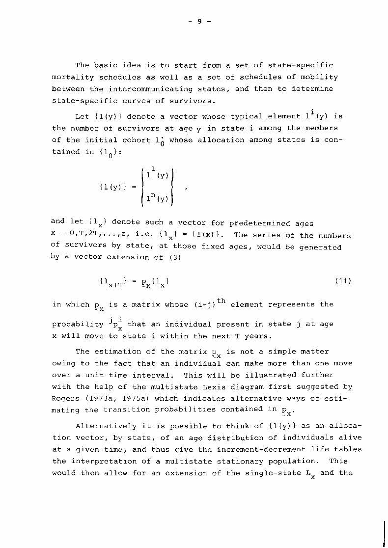
Let {l(y) 1 denote a vector whose typical element li(y) is
the number of survivors at age in state i among the members
of the initial cohort 16 whose allocation among states is con-
tained in {lo}:
and let {lxl denote such a vector for predetermined ages
x = O,T,2T,...,z, i.e. 1 = ( x The series of the numbers of survivors by state, at those fixed ages, would be generated
by a vector extension of (3)
in which p is a matrix whose (i-j) element represents the -X
j i probability px that an individual present in state j at age
x will move to state i within the next T years.
The estimation of the matrix p is not a simple matter -x owing to the fact that an individual can make more than one move
over a unit time interval. This will be illustrated further
with the help of the multistate Lexis diagram first suggested by
Rogers (1973a, 1975a) which indicates alternative ways of esti-
mating the transition probabilities contained in p . , X
Alternatively it is possible to think of {l(y)} as an alloca-
tion vector, by state, of an age distribution of individuals alive
at a given time, and thus give the increment-decrement life tables
the interpretation of a multistate stationary population. This
would then allow for an extension of the single-state Lx and the
derivation of the multistate counterparts of the life table func-
tions defined in ( 6 ) through ( 1 0 ) .
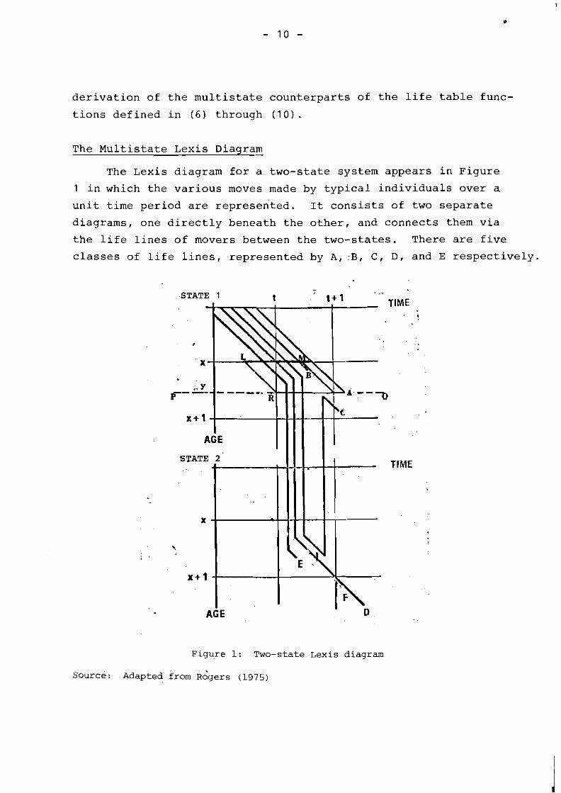
The Multistate Lexis Diagram -
The Lexis diagram for a two-state system appears in ~ i g u r e
1 in which the various moves made by typical individuals over a
unit time period are represented. It consists of two separate
diagrams, one directly beneath the other, and connects them via
the life lines of movers between the two-states. There are five
classes of life lines, represented by A , r B , C, D l and E respectively.
Figure 1: Two-state ex is diagram
source: Adapted £ram ~ G ~ e r s (1975)
Life line A represents the case of an individual surviving in
state 1 who does not move out. Life lines B and E relate to
individuals in state 1 who die during the unit time interval.
In life line B, the death occurs in state 1 while E it takes
place in state 2 after the individual concerned has moved from
state 1 to state 2. Life line C represents the case of an indi-
vidual who moves from state 1 to state 2 and returns before the
end of the age interval. Finally, life line D refers to an
individual in state 1 who moves to state 2, survives the unit
time interval and does not return before the end of the interval.
There are other classes of life lines besides the above that
consist of more than two moves but these are of a lesser impor-
tance. Note that this reasoning can be extended without incon-
venience to the n-state case (the focus on a two-state Lexis
diagram was adopted for ease of exposition).
Alternative Movement and Transition Approaches Contrasted
As mentioned earlier, two main alternative approaches have
been considered to estimate age-specific probabilities such as i j px . Their contrast stems from a different emphasis on the life
lines described by the multistate Lexis diagram.
Suppose we want to determine the matrix pkT consisting of - the various probabilities of surviving through the age interval
(kT, (k + 1 ) T) . As in the single-state life table, the problem
is to define a set of forces of mortality and mobility for any
specific age y(kT - < y - < (k + l)T) and then to proceed to the
age-specific survival probabilities by integration over the whole
age interval.
A first possibility consists of defining age-specific forces
of mortality and mobility out of a given state i at age y by
reference to the group of all individuals present in state i at
that age, no m a t t e r o h a t s t a t e t h e y were p r e s e n t i n a t age x = k T .
For example, such forces of mobility, for age y , out of state 1
of a two-state system concern all the individuals whose life lines
in Figure 1 cross PQ durinq the period ( t , t+l) I i - e - between I
and S.
A second possibility consists of defining state-specific
forces of mobility out of state i by reference to the group of
individuals p r e s e n t i n t h a t s t a t e a t age x = kT. The resulting
forces of mobility for age y out of state 1 of a two-state system,
relate to the group of individuals whose life lines i n Figure 1 , * not only cross PQ (between and S) but also cross LM.
These two alternative de-finitions express two distinct methods
of estimating the age-specific transition probabilities; the
movement approach and the transition approach. In the movement
approach the focus is on moves viewed as events cocurring at
one given point in time. In the transition approach, the emphasis
is on the transitions resulting from the comparison of the states
the individuals were in at two given points in time, regardless
of where the individuals were during the intervening period.
*The forces of mobility defined here allow an individual to move to another region and come back during the span of time elapsing between the crossing of two lines. This contrasts with an alternative definition of the forces of mobility making no allowances for return moves (Hoem, 1 9 7 0 ) .
11. THE MOVEMENT APPROACH
This section presents a complete exposition of the method-
ological and empirical aspects of the construction of increment-
decrement life tables based on the movement approach. It includes
mathematical developments set in both continuous and discrete
terms as well as the applied construction of such tables.
A Theoretical Exposition
In contrast to the single-state case in which one of the
main problems is to follow a unique initial set of babies, the
multistate case requires following babies born in various states
simultaneously.
In the movement approach, this task is carried out by con-
tinuously observing all the movements occurringin the system,
which does not require focusing on fixed age intervals. For
that reason, this approach appears as the more natural way of
extending the single-state life table. This will be confirmed
later when deriving the multistate life table functions that will
appear as straightforward vector or matrix extensions of the
single-state life table functions.
Derivation of the Age-Specific Survival Probabilities
Suppose we have an n-state system in which each state i is
denoted by the index i (i = 1, . . . ,n). Then, as far as state i
is concerned relative to the rest of the system, for an indivi-
dual aged y at time t, three types of demographic events are
possible over the period (t, t + dt):
- survival to age y + dy in state i (dy = dt),
- death before reaching age y + dy in state i, and
- move to one of the other states of the system.
The time interval dt is supposed to be short enough so that
multiple transitions, such as move to and death in a state
j(j f i), are ruled out.
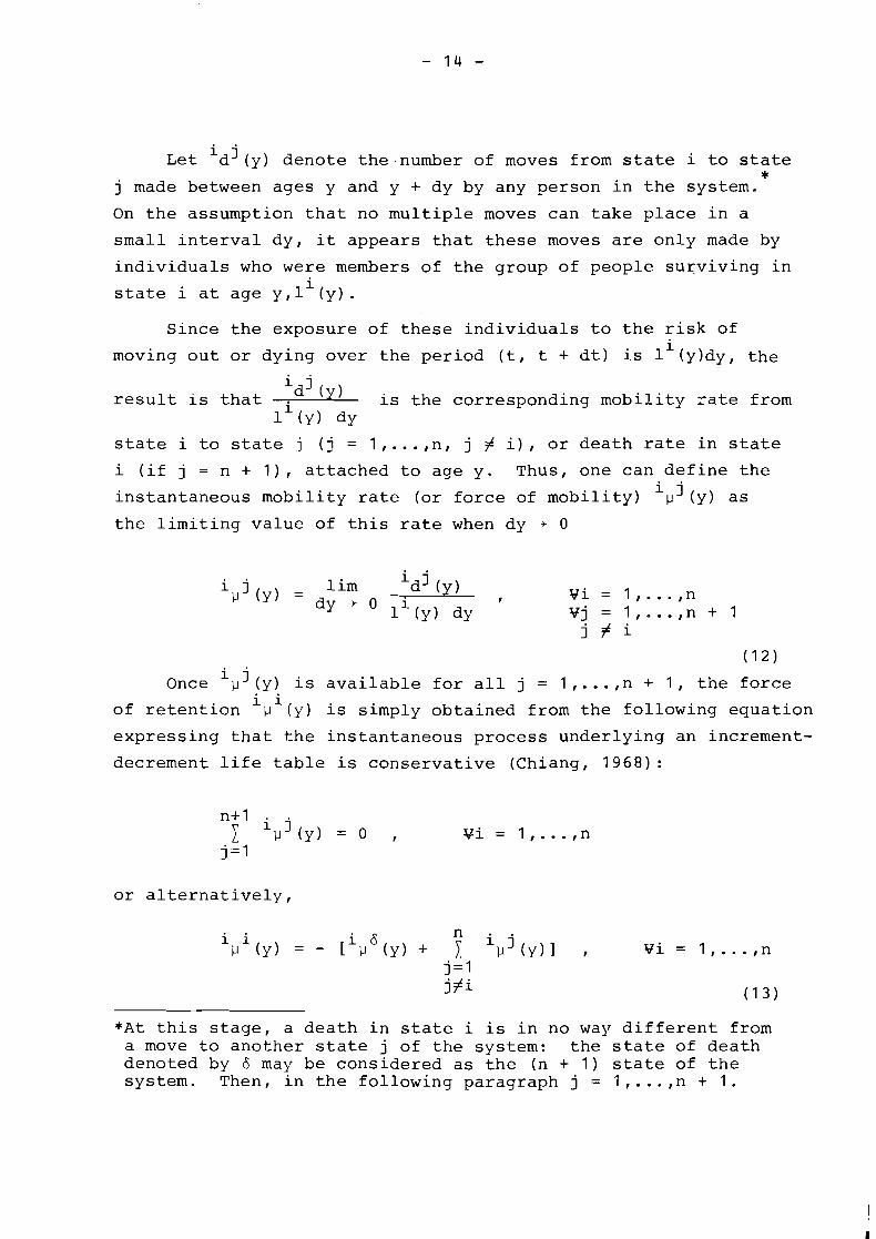
i j Let d (y) denote the.number of moves from state i to state * j made between ages y and y + dy by any person in the system.
On the assumption that no multiple moves can take place in a
small interval dy, it appears that these moves are only made by
individuals who were members of the group of people surviving in i
state i at age y , 1 (y) . Since the exposure of these individuals to the risk of
i moving out or dying over the period (t, t + dt) is 1 (yldy, the
result is that Id' (Y) is the corresponding mobility rate from li(y) dy
state i to state j ( j = 1, ..., n, j # i), or death rate in state
i (if j = n + I), attached to age y. Thus, one can define the i j
instantaneous mobility rate (or force of mobility) p (y) as
the limiting value of this rate when dy + 0
(12) i j
Once p (y) is available for all j = 1, ..., n + 1, the force i i
of retention p (y) is simply obtained from the following equation
expressing that the instantaneous process underlying an increment-
decrement life table is conservative (Chiang, 1968) :
or alternatively,
*At this stage, a death in state i is in no way different from a move to another state j of the system: the state of death denoted by 6 may be considered as the (n + 1) state of the system. Then, in the following paragraph j = 1, ..., n + 1.
As far as the two states i and k = R(i)(i.e.,all states excluding
i) are concerned, there exist the six forces of mortality and . -
mobility indicated in Figure 2(a).
Figure 2. Forces of transition and corresponding movements in a two region system.
Present in state k
k i 11 (Y)
k k 1-1 (Y)
k 6 v (Y)
alive in state i
alive in state k
dead I
Clearly the multistate demographic system determined by the
above definitions is characterized by state-specific mortality
and mobility patterns such that the instantaneous propensity of
an individual to make a move only depends on his age and the
states of origin and destination for this move. In no way, is
this propensity affected by the past mobility history of that
individual or the duration of residence in the state out of which
the move takes place.
Present in state i
i i V (Y)
i k 1-1 (Y)
i 6 1.1 (Y)
li(y + dy)
lk(y + dy)
Present in state k
k i d (y)
-
kd6 (y)
lk (y)
alive in state i
alive in state k
dead
Present in state i
-
i k d (y)
i 6 d (y)
li (y)
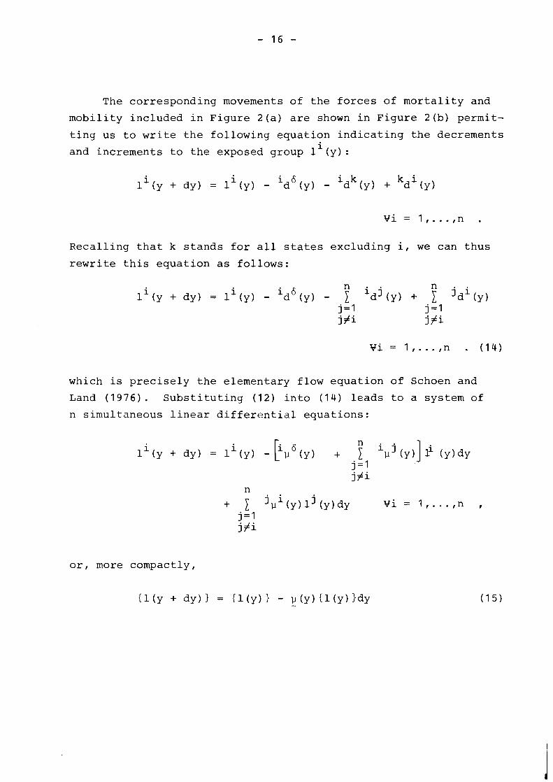
The corresponding movements of the forces of mortality and
mobility included in Figure 2(a) are shown in Figure 2(b) permit-
ting us to write the following equation indicating the decrements i and increments to the exposed group 1 (y):
Recalling that k stands for all states excluding i, we can thus
rewrite this equation as follows:
which is precisely the elementary flow equation of Schoen and
Land (1976). Substituting (12) into (14) leads to a system of
n simultaneous linear differential equations:
or, more compactly,
(1 (Y + dy) = (1 (y) ) - p - (y) (1 (y) )dy
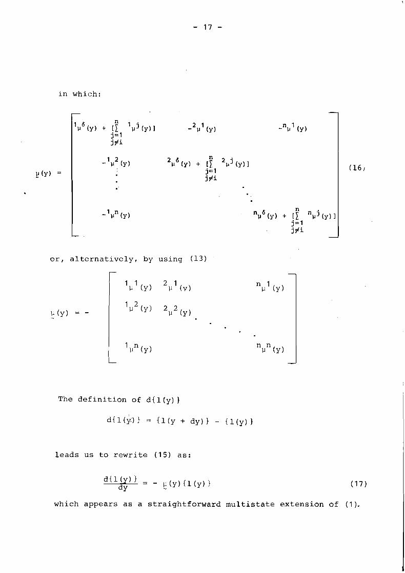
in which:
or, alternatively, by using (13)
The definition of d{ 1 (y) 1
d.{l(y,)l = {l(y + dy)} - {l(y)}
leads us to rewrite (15) as:
which appears as a straightforward multistate extension of (1).
The system defined by (17) admits n linearly independent
solutions {l(y)Ik (k = l,...,n) whose juxtaposition as the columns
of a square matrix yields the integral matrix of the system
(Gantmacher, 1959) :
Since every column of l(y) satisfies (17), the integral matrix - l(y) satisfies the equation: -
From the theorem on the existence and uniqueness of the solution
of a system of linear differential equations, it follows that
l(y) is uniquely determined when the value of l(y) for some - - initial value y = 0 is known, say l(0) or to (Gantmacher, 1959): -
in which the matrix n(y), uniquely defined as the normalized 0-
solution of (18) in that it becomes the unit matrix for y = 0,
is called the matricant (Gantmacher, 1959).
Note that n(y) cannot be simply expressed as a function 0- of the p(y)'s as its counterpart in the basic life table was - in (2) . However, as indicated in Schoen and Land (1 976) and
Krishnamoorthy (1977), it can be determined by using the infini-
tesimal calculus of Voltersa. (Gantmacher, 1959). Such a
determination takes advantage of the following property displayed
by the matricant:
If we divide the basic interval (0 = y 0 f Y = y ) into n parts n
by introducing intermediate points y1,y2r...ryn-1 and set
- Ayk - Yk -
Yk- 1 (k = 1,. . . ,n) , then we have from (20)
If the intervals Ayk are small, we can calculate a (yk) Yk-1-
taking p( t ) Ip(~~) , - a constant matrix, such that Tk is an inter- - mediate point in the intervai (yk - yk). We have:
I
in which the symbol ( * * ) denotes the sum of terms of order two
or greater. Since
we can then rewrite fl (y) as: 0-
Having derived an integral matrix solution of (17), we now
face the difficulty of interpreting it. What is the meaning of
l(y) with regard to the problem on hand? ..,
First let us say that l(y) is a matrix containing n vectors, - each one of them representing an independent solution of (17).
With reference to the "initial" values y = 0, it is clear that
n independent solutions can be obtained by separately generating
the subsequent evolution of the state-specific groups of the
initial cohort 1; . Thus 1O is a diagonal matrix which denotes
the state-specific allocation of the initial cahort: its typical i diagonal element is lo . Furthermore, l(y) is a square matrix -
whose ith column is a vector representing the state specific
allocation of the survivors of li at age y (in the remainder of 0
the paper it will be denoted by 1 (y) ) . 0-
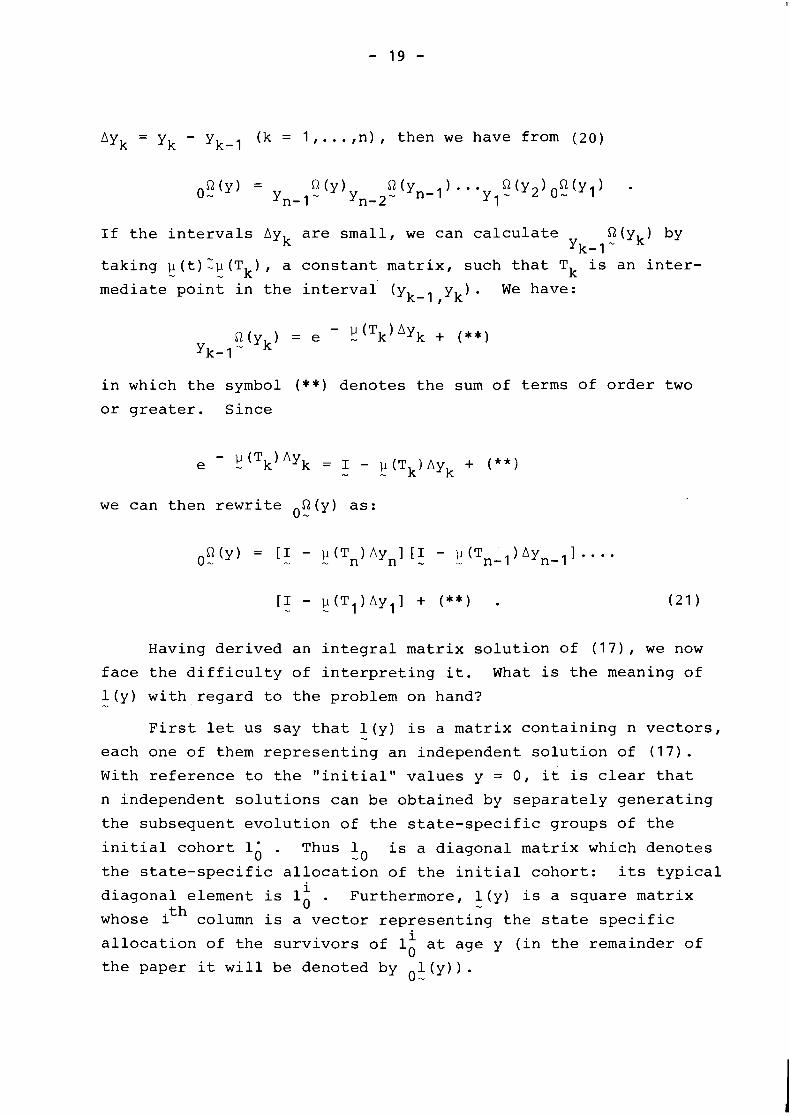
Since the columns of O!(y) are n linearly independent
solutions, their sum is also a solution of (17). Then {l(y))
is given by:
in which {lo) is the allocation vector of the initial cohort 16.
Clearly, the matrix O?(y) defines a set of survival probabilities:
its (i,j) th element represents the probability for a person born
in state j to survive at age y in state i.
From the property (20) of the matricant, it can be concluded i j that the probability px that an individual present at age x
in state i will survive in state j, T years later, is the (j,i) th
element of the matrix p = R(x + T). Hence: ,X X-
An expression of p can be derived from the expressions of -X
R(x + T) and O?(~) obtained by use of the infinitesimal calculus 0- of Volterra:
where x + y l , x + yT.. .,x + ym-l , are (m - 1) intermediate points
dividing the interval (x, x + T) into m parts containing respect-
ively the intermediate points x + el,x + e2,...,x + em-l . *
*Note that the application of the infinitesimal calculus of Volterra, leads us to write
,T -1 p(y * + t)dt n e 0 = I - 1 p (X + ek)Ayk + ( * * ) . Since (23) - -
k= 1
can be rewritten as p = I - -x - 1 p (X + ek)Ayk + ( * * I , one may - k= 1
-lTy (y + t)dt conclude that e 0 is a good approximation of p :
-X the discrepancy represents terms of at least the second order.
Also, note that it is possible to define a matrix q of the -X
probabilities of dying within the next T years analogous to the
x of the single-state life table. Let iqi denote the probability
for a person present in state i at age x to die within the next
T years in state j. Then the number of deaths occurring in state i
j between ages x and x + T for the member of lx is equal to
T i i j x qx as well as to 1 jw6. (x + t) ixlJ (x + t) dt in which
0
ix lJ(x + t) denotes the members of lix surviving to age x + 1 in
state j. Therefore,
- 1
gx = [ jT i(x + t) x- l(x + t)dt] x-x 1 t
0
6 in which ~ ( y ) is a diagonal matrix of instantaneous death rates, -.
i l(y) a matrix whose (it j) th element is 1 (y) and xlx a diago- X- jx - - , - . .
nal matrix whose ith element is 1:. * Finally, substituting (24)
into that last expression leads to: .
or alternatively,
a precise evaluation of which could also be obtained by use of
the infinitesimal calculus of Volterra.
*The notation l(y) generalizes the above notation O1(y) by X-. -. - describing the state changes in the system with reference to the state of the system at any age y (0 < y < x) rather than with reference to the state-of-birth only. Note that (19) can then be gelleralized into
The relevance of Markov processes to the interpretation of
increment-decrement life tables has not gone unnoticed - (Rogers,
&973a, 1975a; Schoen, 1975; Schoen and Land, 1976; Krishnamoorthy,
1977). It is, in fact, simple to -establish that the matrices
of probabilities p determine a Markov transition probability * -X model characterizing the multistate stationary population
defined by {l(y)):
- the matrix px is such that its elements are conditional
upon occupancy of a specific state at age x and are
independent of the history of previous moves or the
duration of residence in the state (this follows from
the property (20) of the matricant) , and
- the elements of p satisfy, as indicated by Schoen and ,x
Land (1976), the three standard conditions specified in
Cox and Miller (1965) : i j
a) 0 5 Px
c) transitivity property defined in (20) . Indeed, the Markov process interpretation is simply due to the
nature of the instantaneous pattern of mortality and mobility
defined by (12). All individuals present at a fixed age in a
given region have identical propensities to move out, indepen-
dent of the past mobility history of each individual.
To summarize, the mortality and mobility process underlying
an increment-decrement life table, characterized by the existence
of a unique survival probability function R(y), leads to an 0-
age-specific distribution {l(y)) that represents a linear com-
bination of n independent age distributions, respectively gen-
erated by each of the state-specific groups of the initial cohort
*The word transition must be understood in its common meaning in stochastic processes. To avoid any confusion, the transi- tion probability matrix p will be referred to as the matrix
-X of survival probabilities.
There are as many linearly independent distributions as non-empty
states in the initial cohort.
Consecluently, ill the multiradix case (more than one state,
possibly n states, al-e initially non-empty), the age-specific
distribution Cl(y)l depends on the state allocation of the initial
cohort. However, in the single radix case (all individuals born
in a unique state), the dge-specific distribution {l(y)} is
uniquely defined.
''his distinctioil is extremely important since
- as we will see later, the multiradix case causes additional
problems with respect to the single radix case in the
discrete formulatioil of the model underlying the con-
struction of an increment-decrement life table, and
- the use of matrix algebra for the derivation of the multi-
state functions is more suitable for the multiradix case * than for the single radix case.
The Multistate Life Table Functions
Two different generalizations of the single-state life table
functions are possible and have given rise to a subject of c9n-
troversy between Schoen and Rogers/Ledent.
The first generalization, introduced by Schoen, consists of
multistate life table functions which are attached to the state-
specific age distributions li (y) considered in their entirety.
*This especially applies to life table functions containing the in- verse of 1
0-x' Clearly, if at least one state of the system is ini-
tially empty, is not invertible. (It contains at least a zero
column and its determinant is thus equal to zero.) However, the formulas containing such a term O;x will remain valid if one re-
duces the scope of the matrices involved: (or more generally
any matrix to be inverted) will be reduced to a r x r matrix (in which r is the number of states initially empty), while the other matrices will be reduced to s x r matrices (in which s is not necessarily equal to r:r 5 s < n). -
Schoen and Nelson (1974) define:
as a function which, like the Lx variable in the single-state
life table, has a dual meaning. It represents first the number
of people alive in state i of the increment-decrement life table
between ages x and x + T, and second, the number of person-years
lived by the initial life table cohort 1; in state i between
those ages. (26) can be rewritten in a vector format as:
We can define ET(x)), the state-specific allocation vector
of the number of people alive in the life table aged x and over,
as:
With the idea of extending the definition (7) of expecta-
tions of life at exact ages, Schoen and Land (1976) define the
mean duration of stay in a given state after age x for all sur-
vivors in the system at age x as,
This is a statistic that we would like to further qualify by
state of presence at age x. However, this is not straightforward
since the person-years lived included in the quantities T: in-
volve members of 1; as well as members of all the groups
1' (j = 1 , . . . , n , j # i . We need to have recourse to variables X
i such as ej denoting the number of years that a member of lx ix x can expect to spend in region j before his death. We then have
the following equation linking 1, e and T functions.
or more compactly,
e {lxl = {Txl X-X
in which the (i, j ) th element of e is e i x-x jx x
This vector equation (27) is clearly insufficient to draw
e from the availability of 11 1. However, it suggests that X-X -x the generation of n linearly independent {l(y)) distributions,
would allow for a derivation of e . Let {lx}, denote the age- X-X
distribution relating to the first increment-decrement life table
generated and { T ~ } ~ the corresponding number of person-years
lived over age x. Thenlit is possible to write
e 1 = T X-X -X -X
in which
1 -x = [{lxllf..,{lxjn] and T ?.x = [ {T~}~,. . . , {T~~~] ,
which leads to:
In fact, the generation of n linearly independent increment-
decrement life tables is nct necessary to obtain xex. Let us
recall that the differential equation (17) underlying an increment-
decrement life table admits n linearly independent solutions
corresponding to n initial cohorts, each of which has a radix
concentrated in a different state. Then, i't suffices to attach an
additional subscript referring to the state of birth to define
multistate life table functions leading to the derivation of
e (Rogers 1973a, 1975a). X-X
The second generalization of the single-state life table
functions thus starts with ;he definition of O ~ i '. It repre-
sents the number of people born in j and alive in state i of the
life table between ages x and x + T, which is also the number
of person-years lived in state i between those ages by the
members of the initial cohort born in state j as:
whi.ch can be written more compactly as:
The total number of person-years lived in state i in prospect
for the group born in j may be taken as
or, more compactly:
The superiority of this matrix generalization of the single
life table Lx is evident in that, unlike the vector generalization
(Schoen) , it permits a direct derivation of e from (28) re- X-X
written as:
- 1 e = T 1 x-x 0-x 0-x
Note that on substituting (30) into that last equation and - 1 replacing 1 (x + t) 1 0-x
R (x + t) yields 0- by x-
e = J x-x
R(x + t)dt X-.
0
an expression that indicates the independence of w" vis-a-vis
the state allocation of the initial cohort. Rogers (1975b) also
develops the notion of a net migraproduction matrix as an alter-
native measure of mobility. Specified in a discrete setting,
the latter expresses mobility in terms of the number of expected
moves out of each state of the system beyond some given exact
ages O,T,2T, ..., z . Below, we re-examine this concept using a
continuous specification. nJ be the number of moves that Let ix x
an individual present at age x in region i can expect to make
nj is the total out of state j before his death, then 1 iOlx kx k -
i number of moves that the members of lo can expect to make out
of state j beyond age x.
Alternatively, this number can be obtained by applying the n
total mobility rate 1 jpk(x + t) to iolJ (x + t) for the k= 1 k#j
t > 0, and summing them: -
which can be expressed more compactly as:
mt n 1 = j p ( ~ + t ) ~ l ( x + t ) d t x-x 0-x - - 0
in which n is a net migraproduction matrix whose (i,-j) th X-X
i mt element is jxnx and p (x + t) a diagonal matrix whose i
th -
n i k diagonal element is [ 1 p (x + t)] . Consequently
k= 1 kfi
03
mt n = [ I p ( x + t ) o l ( ~ + t)dtl 1 - 1
X-X - - 0-x
On substituting C2 (x + t) for 1 (x + t) 1 (x)-' x- 0- 0- yields,
an expression that also shows the independence of x> vis-a-
vis the state allocation of the initial cohort.
Another consequence of the matrix notation is the possib-
ility of extending the definitions (29) and (30) by relating the
multistate functions to the states of presence at any age y
rather than to the state-of-birth. For example, L denotes amatrix Y -x
T whose typical element Li =
jy x i jy li(x + t)dt is the number of
0
people present at age y in state j (0 < y L x) and alive in state - i between ages x and x + T. In a similar way, T denotes a
Y -x 03
matrix whose typical element T~ = I j~ li (x + t)dt is the total
jy x 0
number of years that a person present at age y - i n state j can
expect to live in state i beyond age x.
It can immediately be established that the following rela-
tionships extending (31) and (33) hold:
- 1 e = T L x-x y-x y-x I Q O Z Y < X -
a3
n = [ j m:(x + t) 1(x + t)dt] 1 -1
X-X - Y- Y -x I Y y O < y z x - 0
Note that this generalization of the multistate life table func-
tions, focusing on the states of presence at any age rather than
on states of birth, is very useful. As mentioned earlier, in the
case of a system with some initially empty states, the knowledge
of 1 and L only permits the calculations of expectations of 0-x 0-x life or migraproduction rates at any age relating to the initially
non-empty states. Fortunately, the knowledge of xlx and L X-X
and the use of the just derived formulas permit deriving those
statistics relating to all states which are initially empty but
non-empty at age x.
It is also possible to extend the two alternative measures
of mobility (expectations of life and migraproduction rates)
by defining them with reference to the state of presence at
age y (0 5 y 2 x). This leads to a matrix of expectations of
life e by place of presence at age y defined as Y-x
mt e = T 1 - 1 y-x y-x y-x
mt in which 1 is a diagonal matrix whose typical element is
Y-x n k 1 . In a similar way, one may define a matrix of migra- i y x k= 1
production rates yax by place of presence at age y as
Note that, if y is zero, the above definitions reduce to those
of expectations of life and migraproduction rates by place-of-
birth put forward by Rogers (1 975a) . *
*All types of expectations of life and migraproduction rates are independent of the state allocation of the initial cohort. We can establish the following relationships between the multistate functions just defined:
e = e Q(x) , n = 0-x x-x 0- n R(x)
0-x x-x 0-
and e n - 1 - - e n - 1 0-x 0-x X-X X-X
Age-specific Mortality/Mobility Rates and Survivorship Pro~ortions
The extension of the age-specific death rate mx of the
single-state life table is straightforward in the present version
of the multistate life table. The age-specific movement rate - -
i j imJ the discrete counterpart of 11 (y), is defined as the ratio X' - . - .
of the number of moves from i to j between ages x and x + T
to the expose,d population L::
i j From the definition (12) of the instantaneous rate uX(y) r it
follows that the number of movements is equal to
and substituting into the above definition yields:
It is clear that the above definition of the age-specific rates
involves the consideration of all persons (whatever their state
of birth) alive in the system between ages x and x + T. Conse- i j
quently, the value of m is affected by the state allocation of X
the initial cohort as indicated by this equivalent specification * of (35) :
i j * This specification of m also shows that unlike the instantan- X
eous mortality and mobility rates which are independent of each other, the discrete mortality and mobility rates are not indepen- dent within and between regions.
A further consequence of this dependence of the age-specific
mortality/mobility rates on {l ) is the impossibiiity of drawing 0
the age-specific movement rates from the life table functions,
as can be done in the single-state case. The discrete equivalent
to the elementary flow equation (14) can be written .as:
Substituting the definition equations (35) then leads to:
which can be rewritten as:
{lx+Tl = {Ix) - m {Lxl -.x
in which m is the discrete counterpart of (161, i.e., -X
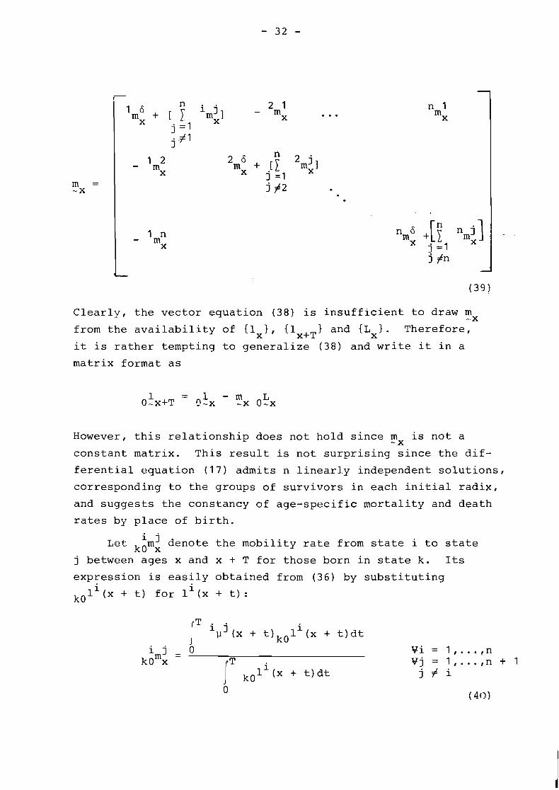
Clearly, the vector equation (38) is insufficient to draw mx - from the availability of {lx}. {lx+T } and {L~}. Therefore,
it is rather tempting to generalize (38) and write it in a
matrix format as
However, this relationship does not hold since m is not a -X
constant matrix. This result is not surprising since the dif-
ferential equation (17) admits n linearly independent solutions,
corresponding to the groups of survivors in each initial radix,
and suggests the constancy of age-specific mortality and death
rates by place of birth.
i j Let kOmx denote the mobility rate from state i to state
j between ages x and x + T for those born in state k. Its
expression is easily obtained from (36) by substituting
kO li (x + t) for li (x + t) :
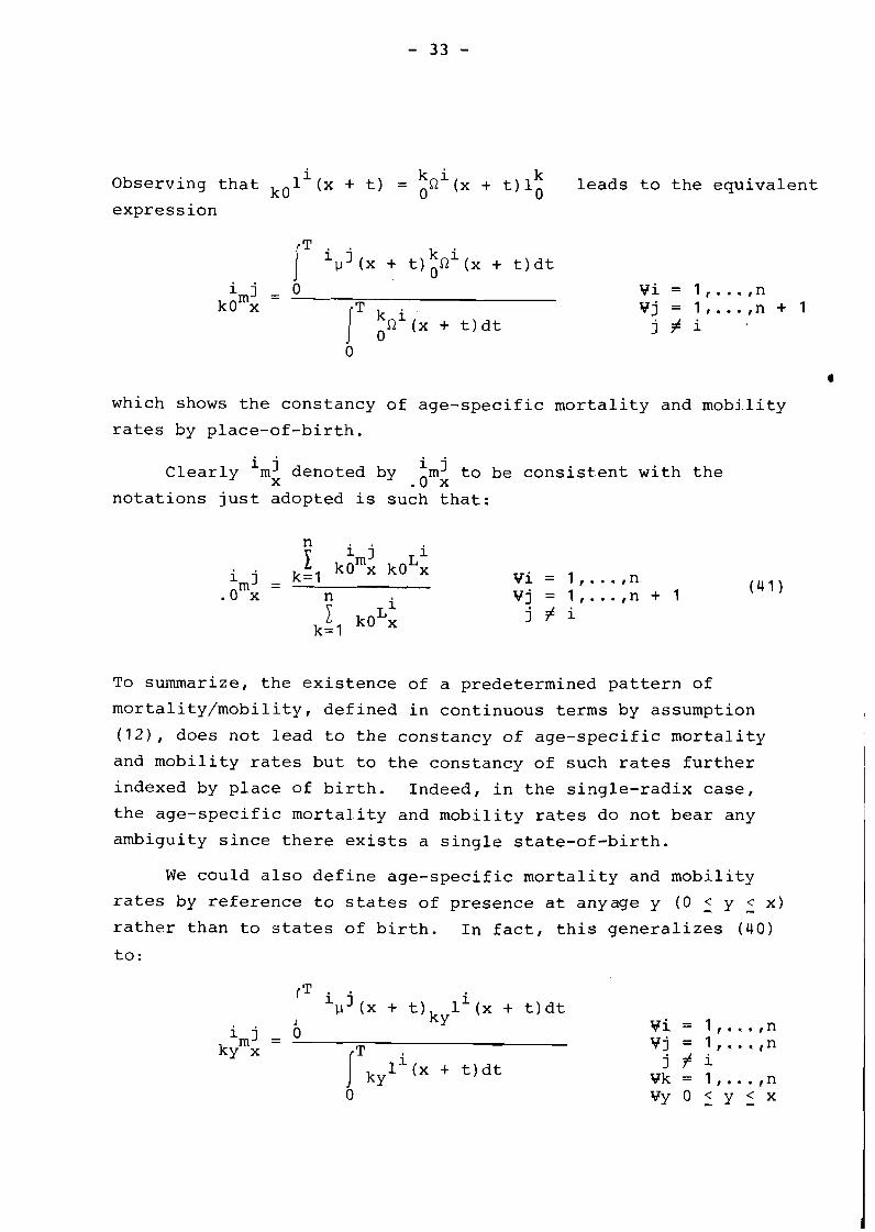
k i Observing that kOli(x + t) = f2 (x + t)l 0 leads to the equivalent
0 expression
0
* which shows the constancy of age-specific mortality and mobility
rates by place-of-birth.
Clearly imL denoted by imJ to be consistent with the .o x notations just adopted is such that:
Yi = 1, ..., n Yj = l,.. .,n + 1
(41
j f i
To summarize, the existence of a predetermined pattern of
mortality/mobility, defined in continuous terms by assumption
(121, does not lead to the constancy of age-specific mortality
and mobility rates but to the constancy of such rates further
indexed by place of birth. Indeed, in the single-radix case,
the age-specific mortality and mobility rates do not bear any
ambiguity since there exists a single state-of-birth.
We could also define age-specific mortality and mobility
rates by reference to states of presence at anyage y (0 2 Y 2 x)
rather than to states of birth. In fact, this generalizes (40)
to:

and (41) to:
Note the dependence of these rates on the state allocation of
the initial cohort.
Another life table function that one would like to extend
to the multiregional case is the survivorship probability s X
denoting the proportion of individuals aged x to x + T who
survive to be x + T to x + 2T, T years later.
For example, we define the proportion of individuals
present in state i between ages x and x + T who move to state
j and survive to be included in that state's x + T to x + 2Tyears
old population T years later, then
which can be written more compactly as:
j i in which s is a matrix whose (i, j ) th element is sx -
-x
Again (42), a vector equation, is insufficient to draw
s from the availability oC the multistate stationary population -X {Lx}. Furthermore, it suggests that the survivorship proportions
depend on the state-specific allocation of the initial cohort.
Then, as is the case of the age-specific mortality and mobility
rates, it is necessary to characterize the survivorship by a . . third index relating to the state of birth. Let 's3 denote
k kO x the proportion of kOLx who move to state j within a T-year period.
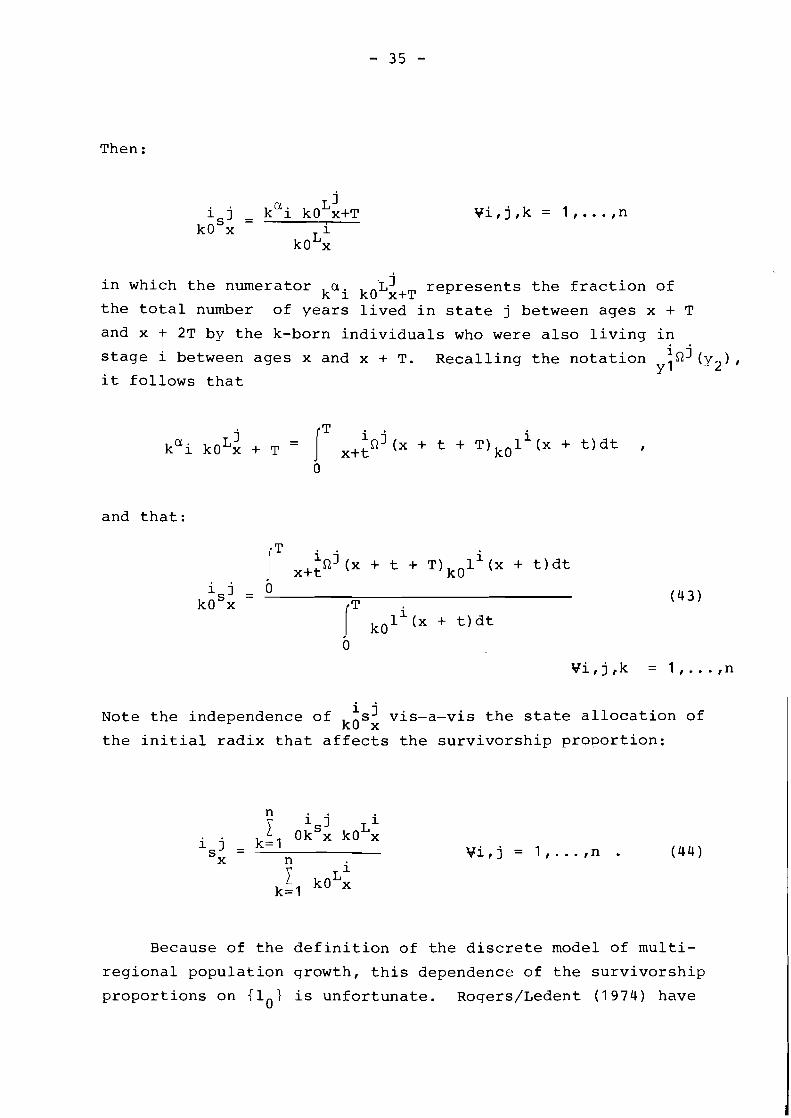
Then:
in which the numerator kai kO-~i+T represents the fraction of
the total number of years lived in state j between ages x + T
and x + 2T by the k-born individuals who were also living in i ' stage i between ages x and x + T. Recalling the notation n1 ( y 2 ) , Y 1
it follows that
and that:
Note the independence of isJ vis-a-vis the state allocation of kO x
the initial radix that affects the survivorship proportion:
Because of the definition of the discrete model of multi-
regional population growth, this dependence of the survivorship
proportions on {lo} is unfortunate. Rogers/Ledent (1974) have
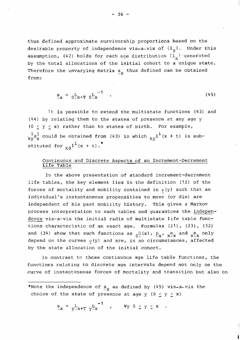
thus defined approximate survivorship proportions based on the
desirable property of independence vis-a-vis of {lo}. Under this
assumption, (42) holds for each aqe distribution {lx} generated
by the total allocations of the initial cohort to a unique state.
Therefore the unvarying matrix s thus defined can be obtained -x from:
It is possible to extend the multistate functions (43) and
(44) by relating them to the states of presence at any age y
(0 - < y 5 x) rather than to states of birth. For example,
isJ could be obtained from (43) in which li(x + t) is sub- ky x * ky stituted for kOli (x + t) .
Continuous and Discrete As~ects of an Increment-Decrement Life Table
In the above presentation of standard increment-decrement
life tables, the key element lies in the definiti~n (12) of the
forces of mortality and mobility contained in ~ ( y ) such that an - individual's instantaneous propensities to move (or die) are
independent of his past mobility history. This gives a Markov
process interpretation to such tables and guarantees the indepen-
dence vis-a-vis the initial radix of multistate life table func-
tions characteristic of an exact age. Formulas (21), (23), (32)
e and n only and (34) show that such functions as 0? (x) , E~ , x-x X-X
depend on the curves ~ ( y ) and are, in no circumstances, affected - by the state allocation of the initial cohort.
In contrast to these continuous age life table functions, the
functions relating to discrete age intervals depend not only on the
curve of instantaneous forces of mortality and transition but also on
*Note the independence of s as defined by (45) vis-a,vis the - X choice of the state of presence at age y (0 - < y 5 x)
L - I s = L x y-x+T y-x I u y o z y < x . -
state/age distribution of the resulting stationary population.
Since the latter is determined by the same curves of instantaneous
forces and by the state allocation of the initial cohort, as shown
by (19), it follows that m and ths matrix of true survivorship -X
proportions s are affected by the state allocation of i; . 5X
Nevertheless, the pattern of mortality and mobility is such that
constant mortality/mobility rates and survivorship proportions
can be found in each of the multistate stationary populations
originating from each state-specific group of the initial cohort.
The assumption of (12), defining the instantaneous mortality
and mobility pattern,leads to constant age-specific mortality and
mobility rates for each of the multistate stationary populations
generated from the n independent solutions of (17). Note that,
although the forces of mortality and mobility depend only on the
states of origin and destination, the age-specific mortality and
mobility rates "by state of birth" depend on all states in the
models as suggested by (40). Consequently, for a given x , the
matrices k0mx for all k = 1, ..., n are not independent. The im-
portance of this finding will be made clear later.
Multistate Life Table Functions in Terms of the Life Table Mortality and Mobilitv Rates
The above exposition of increment-decrement life tables sUq-
gests that a point of choice in proceeding from the life table
age-specific mortality and mobility rates is the integration of
{l (y) 1 and 0t (y) over successive intervals (x, x + T) . As in the
single-state case, this problem can be illustrated further, even
without supposing any explicit methodfor deriving {L~). This
requires the consideration of a matrix a of mean durations of -X
transfers. It is the multistate analog of the average number of
years a lived in the interval (x, x + T) by those of the single- X
state life table who died in that interval.
The Matrix of Mean Durations of Transfers over a ~ i m e Period
In order to understand the matrix of mean durations of tran-
fers over a time period, it is sufficient to focus on the subsequent
evolution of the group of people between ages x and x + T present
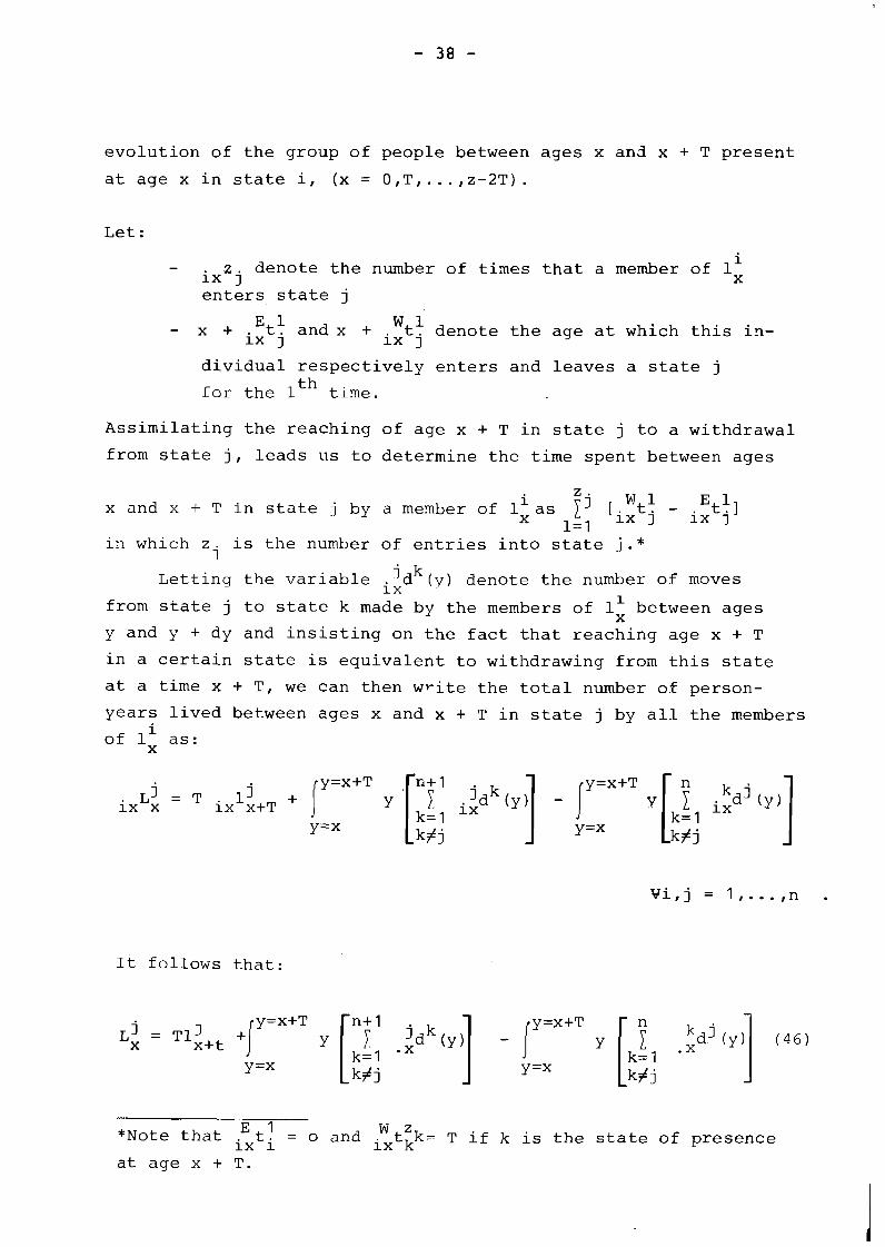
at age x in state i f (x = O,T,. . . ,z-2T).
Let:
- i z denote the number of times that a member of 1
ix j x enters state j
- x + Etl and x + 'tl denote the age at which this in- ix J ix J
dividual respectively enters and leaves a state j
for the lth time.
Assimilating the reaching of age x + T in state j to a withdrawal
from state j, leads us to determine the time spent between ages
z i Wtl - x and x + T in state j by a member of 1 as 1' Lix ix , 1=1
in which z is the number of entries into state j.* i
Letting the variable i?dk(y) denote the number of moves
from state j to state k made by the members of 1: between ages
y and y + dy and insisting on the fact that reaching age x + T
in a certain state is equivalent to withdrawing from this state
at a time x + T, we can then write the total number of person-
years lived between ages x and x + T in state j by all the members i
of lx as:
It follows that:
w z *Note that Lt: = o and ixtkk= T if k is the state of presence
at age x + T.
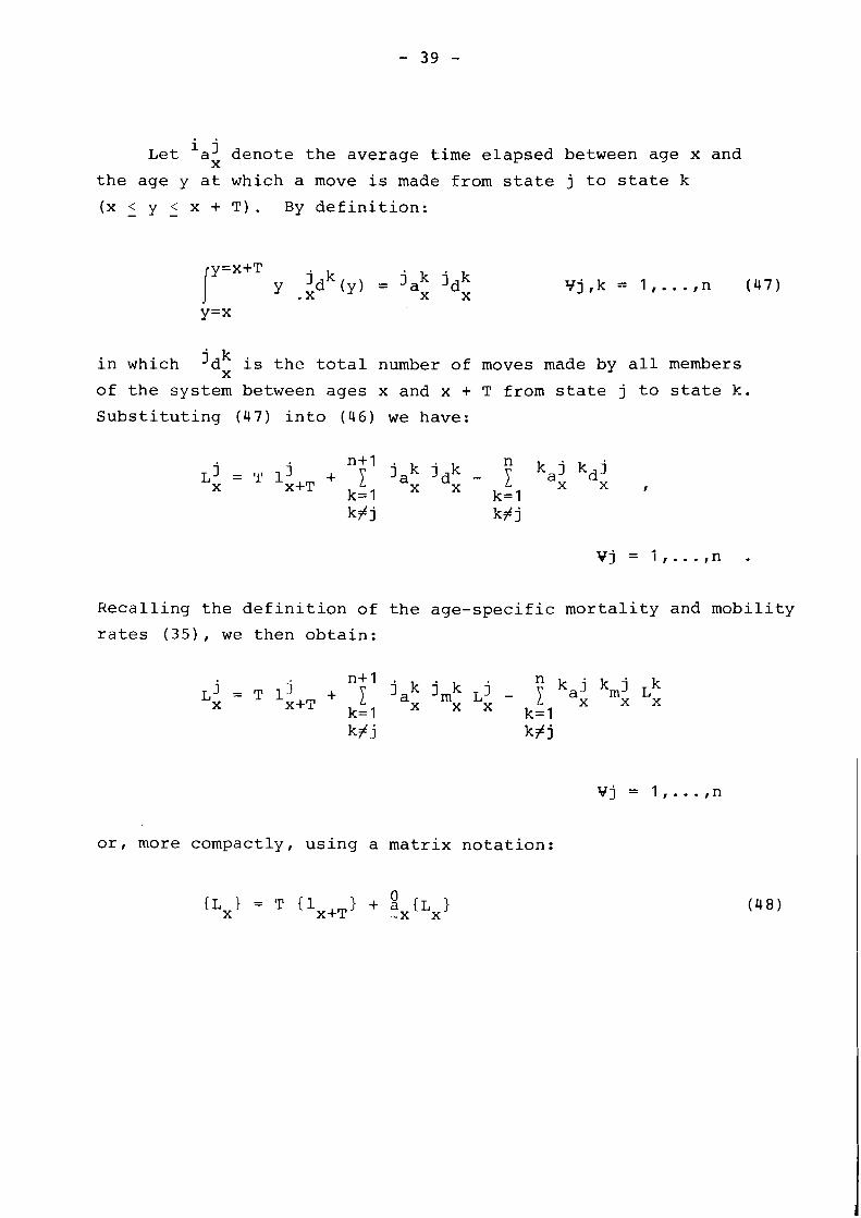
i j Let ax denote the average time elapsed between age x and
the age y at which a move is made from state j to state k
(x - < y - < x + T). By definition:
in which Idk is the total number of moves made by all members X
of the system between ages x and x + T from state j to state k.
Substituting (47) into (46) we have:
Recalling the definition of the age-specific mortality and mobility
rates (35) , we then obtain:
or, more compactly, using a matrix notation:
-X
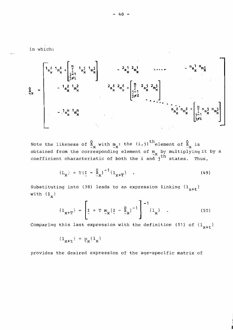
in which:
0 th 0 Note the likeness of a with mx: the (i,j) element of a is -X - -X
obtained from the corresponding element of m by multiplyingit by a -X
coefficient characteristic of both the i and jth states. Thus,
Substituting into (35) leads to an expression linking (1 1 x3t with {lxl
Comparing this last expression with the definition (11) of (1 ) x+t
provides the desired expression of the age-specific matrix of
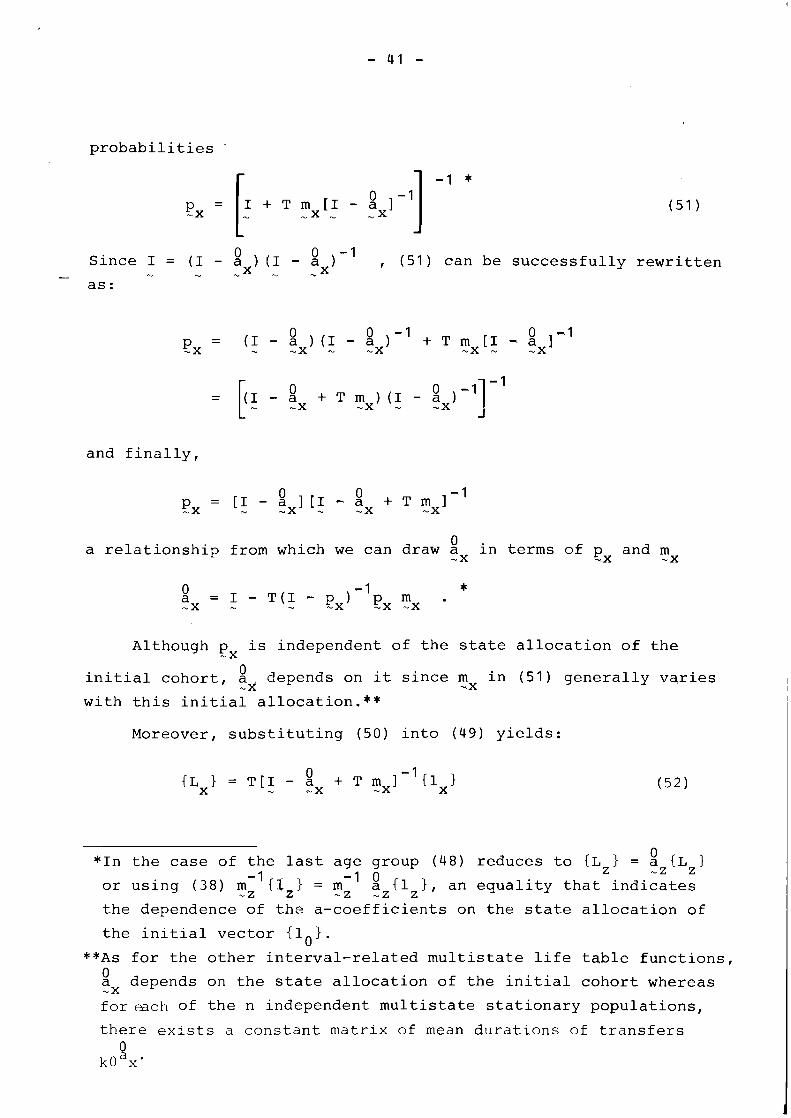
probabilities '
0 0 -1 Since I = (I - ax) I1 - ax) , (51) can be successfully rewritten - - - - - -
as:
and finally,
0 a relationship from which we can draw ex in terms of p and m ?.x -X
Although p is independent of the state allocation of the -X
0 initial cohort, ax depends on it since m in (51) generally varies -X
with this initial allocation.**
Moreover, substituting (50) into (49) yi.elds:
0 *In the case of the last age group (48) reduces to {L 1 = a {L 1
-1 0 Z -Z Z
or using (38) m ~ ' - {IZ} = m aZ{lZ} , an equality that indicates -Z -
the dependence of the a-coefficients on the state allocation of
the initial vector {lo}.
**As for the other interval-related multistate life table functions, 0 a depends on the state allocation of the initial cohort whereas -X for each of the n independent multistate stationary populations,
there exists a constant matrix of mean durations of transfers
an expression that will later allow the derivation of q . Since -X
those who die in state j between ages x and x + T were members k
at age x of any cohort lx, the corresponding number of deaths can
n k j k L' so that we have in matrix be written either qx lx or mx k= 1
6 8 form q llx} = m {Lx} in which mx is a diagonal matrix of death -X -x -
rates. Substituting the expression of {L into this last for- x mula then leads to:
and finally, because of the independence of q from {Ix], we have -X
The Case of a Uniform Distribution of All Moves
Before looking at the case of a uniform distribution of moves,
let us consider the case in which all moves out of a region are
similarly distributed. Then:
0 which permits us to express ax as the product of two matrices:
i in which a is a diagonal matrix whose typical element is a . -x X In such circumstances, ( 4 8 ) becomes
After substitution of ( 3 8 )
becomes a formula generalizing the single-state identity
The single-state function a is extended as the more complex X - 1
function m a m ; the latter however, reduces to ax if all moves -X-X-X
in the system are uniformly distribut.ed. Substituting the expres-
O into (51) and (53) yields: sion of ax
-1 = [I - m a ] [ I + m ( T I - a )I Px - -X-X - -X - -X
(5 5
and
Note that (55) corrects the formula given in Rogers/Ledent (1976)
in which the two expressions between brackets were inverted.
Furthermore, if all moves out of each region are uniformly
distributed for each closed interval, i.e.,
a = - I -x 2 -
for all x f z , (57)
we obtain by substitution into (55)
T T T T * [_ I - - m ][I + - m 1 = [I + - m ][I - - m I, 2 -x - 2 -x - 2 -x - 2 -x Px
can be rewritten
as : T T
Px = [I + mx1-' [I - - m 1 (58a). - 2 -x
This alternate expression of p is found in Rogers/Ledent (1976). -x
and by substitution into ( 5 6 )
Conversely from (58) we can draw an expression of mx in terms of - Px
an equation which indicates that m is uniquely defined in terms -x
Px and is thus independent of the state allocation of the
initial vector.
Consequently, assuming a uniform distribution of moves, we
find constant age-specific mortality and mobility rates by place-
of-birth for any choice of the state allocation of the initial
cohort, i.e.,
Then, (38) can be generalized as:
an equation from which we can draw
As in the single-state case, the assumption of uniformly dis-
tributed moves leads to the derivation of survival probabilities
that are identical to those obtained by supposing a linear integra-
tion over {Ix). This result can bedemonstrated directly by comparing
* ( 6 1 ) also holds if the multistate life table rates relate to the state of presence at age y ( 0 < y < x) rather than to state - - of birth:
= imJ = constant independent of y ( 0 < y < x) and k(= 1, ..., n). ky x X - -
T {Lx} and2[{lx} + {1,+~}1 . Assuming (57) yields
and
T T -1 Since I can be decomposed into (I + !X) (I + - m ) this even- - - - 2 -x tually leads to:
T Setting a = - I in (52) gives -x 2 -
and consequently we obtain after comparing (62) and (63)
Conversely, if one assumes that {Lx} is given by a linear inte-
gration such as (64) for any choice of the state allocation of
the initial matrix, one finds by comparing (38) with (64) that:
Further comparison with (51) leads to
showing that all movements are uniformly distributed in each
age group.
In other words, as in the single-state case, the assumption
of a uniform distribution of movements is equivalent to .the
linear derivation of the person-years in the stationary population.
This equivalence,shown here by reference to the vectorial
age distributions, also applies to the matrical age distributions
Since m is independent of the initial radix, the matrix exten- -X
sion of (64) holds, giving
a relationship which permits us to obtain the values of Rogers'
multistate life table functions such as OTxfx'x from the knowledge * of mx. -
Carrying the linear integration on 11 is equivalent to X
performing it not only on L but also on L (for all y, 0 5 y 5 x). 0-x Y -x This finding permits us to compute some of the multistate functions
relating to initially empty states by using the generalized expres-
sions of multistate life table functions relating to states of * * presence at age y rather than to states of birth.
*In addition, the property of independence displayed by m allows -X
rewriting (33) in a discrete form as:
m m t L 1 - 1 n = X-X -X 0-X 0-X
n i k in which %! is a diagonal matrix whose ith element is [ 1 mxl , - x k= 1
kfi thus making it possible to express n in terms of the life table
X-X rates.
**This observation is important as the non equivalence of the cubic
integration 05, and L will suggest later. Y -x
In the case of the terminal age interval which is half open,
a different treatment is used:
- Pz is set to zero since everybody eventually dies, and
- since the length of the interval is infinite, okZ cannot
be obtained by linear integration.
For this age group, we assume the independence of the life
table mortality and mobility rates vis-a-vis the state allocation
of the initial cohort, a property equivalent to the linear inte-
gration hypothesis in the case of the closed age intervals. Thus
(60) in which OAZ+T = 0 holds, leads to
Thus,
- 1 = L - 1 e = T 1 x-z 0-2 0-2 9-z 0-2 - z
Note that mZ being independent of the state allocation of the - intial vector,
is an equality giving:
In other words, the assumption made about mZ is equivalent to - supposing that in the last interval, all moves (except deaths)
out of a region, take place instantaneously at exact age z.
*This formula. is the matrix expression of the various scalar formulas derived by Schoen in the appendix of his 1975 article. Also, note that mZ is not a diagonal matrix: non-zero mobility - rates are here allowed, unlike in Rogers ( 1 9 7 3 a ) .
The derivation of the true survivorship probabilities by
state of birth as defined by ( 4 3 ) requires a further assumption
concerning the integration of the numerator. We can use a linear
integration method which would be consistent with the method of
integration used for deriving {L~}, then:
By contrast, because of the linear integration assumption for
deriving {Lx}, the approximate survivorship probabilities as
defined by ( 4 5 ) can be simply expressed in terms of the age-specific
mortality and mobility rates.
From ( 6 5 ) rewritten as
it follows that:
and eventually, after substitution of ( 5 5 ) for the age-specific
probabilities:
The comparison of ( 6 7 ) with ( 5 8 ) suggests that s is simply ob- ?X
tained from the formula giving p by replacing the age-specific -x matrix m within the first brackets with the similar matrix mx+T
-X - corresponding to the next age group.
Of course, (67) is valid only for x = O,T, ..., z-2T whereas
S -z-T is given by:
obtained by combining (45) , (55) , ( 6 5 ) t and (66)
Another statistic needed in Section I11 is the matrix which
gives the regional allocation of survivors at time t + T among
those born between times t and t + T.
If a child is born in state i at time tl (0 < tl < T since
we can suppose t = 0 without imposing any further restriction),
the possibility he or she will live to the end of the interval
1' iO x-tl (age T - t ) i.n state j is 1 . Summing this through the . i T-year interval of time and age, with births uniformly distributed
in time within the T years, gives the proportion of survivors
in state j among children born throughout the interval in state
Then we have,
and since
we obtain:
The similarity mentioned above between the formulas giving the
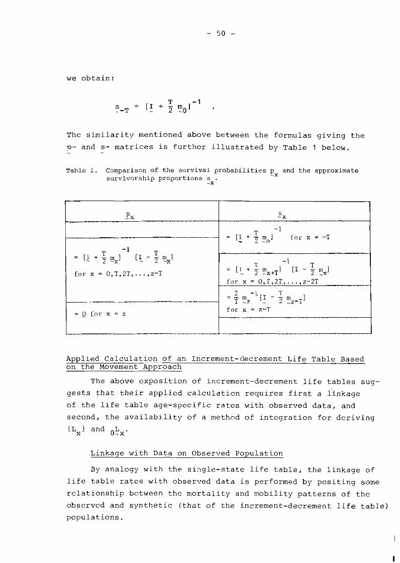
g- and s- matrices is further illustrated by Table 1 below. - -
Table 1. Comparison of the survival probabilities p and the approximate - x survivorship proportions s . - X
Applied Calculation of an Increment-decrement Life Table Based on the Movement Amroach
,Px -
T - 1
- T - [ : + - m ]
2 -x [I- - "1
f o r x = O,T,2T, ..., z-T
= Q f o r x = z
The above exposition of increment-decrement life tables sug-
gests that their applied calculation requires first a linkage
of the life table age-specific rates with observed data, and
second, the avai1abj.li.t~ of a method of integration for deriving
{ L ~ } and L . 0-x
s - X
T - 1 - - [ I + - m l f o r x = -T 2 -0
T - 1 - T - [ I _ .+ T [I - cxl f o r x = O , r , 2 T , ..., z-2T
2 -1 = - m T T - Z [I - ? ~ z - T ]
f o r x = z-T
Linkage with Data on Observed Population
By analogy with the single-state life table, the linkage of
life table rates with observed data is performed by positing some
relationship between the mortality and zobility patterns of the
observed and synthetic (that of the increment-dzcrement life table)
populations.
-
As presented above, increment-decrement life tables are
based on the predetermined knowledge of mortality and mobility
patterns defined by continuous curves of such forces. Ideally,
one should carry out the linkage with the observed population
system by assuming identical curves of mortality and mobility forces
in both the synthetic and observed pcpulations. However, the
difficulties encountered-in implementing such an assumption when
calculating an applied life table, make it necessary to link ob-
served and life table patterns of mortality and mobility at a
discrete level.*
Then, as in the single-state case, we are left with relating
life table age-specific mortality and mobility rates to observed
data. But, is it possib1.e to implement a linkage analogous to the
one of the single-state life tables in which a simple equality of
the age-specific mortality rates of both the life table and observed
populations is generally posited?
Earlier, we pointed out that the assumptions underlying
movement increment-decrement life tables led to n elementary
multistate stationary populations, characterized by constant age-
specific rates. In addition the consolidated stationary population
displayed age-specific rates varying with the state allocation of
the initial cohort. Consequently, the most efficient strategy
would be to estimate age-specific mortality and mobility rates by
*The generalization of two single-state methods assuming identical curves of mortality and mobility forces are possible: (1) a method iterating to the "data" analogous to the method
proposed by Keyfitz (1968, Chapter I), and (2) a method extending that of Keyfitz and Frauenthal (1975).
Although no attempt to evaluate and compare the validity of these two methods was undertaken, it can be said that the former alternative is feasible, whereas the latter, studied by Krishnamboodiri (1977) is likely to lead to highly inaccurate results. The rationale for this a ~ r i o r i judgement is that the curves of instantaneous mobility forces encountered in multistate models are not as nicely shaped as the curves of instantaneous forces of mortality in the single-state life table.
state of birth for the actual population and to equate them to
their life table counterparts. Unfortunately, for most choices
of the integration method for deriving {Lx), this would yield age-
specific survival probabilities different for each one of the
n elementary stationary populations since the age-specific rates
of these populations are not independent.
Under these conditions, the only practical way to proceed is
to reduce the generality of the increment-decrement life table by
further assuming that all types of moves out of each state are
evenly distributed and that the typical distribution is independent
of the state allocation of the initial cohort. This is equivalent
to imposing identical life table age-specific rates in each elem- * tary stationary population.
On imposing the above restriction, the calculation of movement
increment-decrement life tables is greatly simplified since:
- the equality of the life table and observed rates of
mortality and mobility no longer raises a problem, and
- matrix generalizations of vector equations such as ( 3 8 ) ,
and ( 5 4 1 , now hold.
From there, the applied calculation of multistate life table func-
tions still requires amethod of integration for deriving {Lx).
The most common way to proceed is to assume a uniform distribution
of these moves over time (linear integration). The columns of
increment-decrement life tables directly follow from the applica-
tion of formulas that pertain to the linear case in which the
matrices of age-specific life table rates are set equal to their
observed counterparts.
Two of the most popular alternatives to the linear integra-
tion method are, in the single-state case, a cubic integration
method and an interpolative-iterative procedure. Can these methods
be extended to the standard approach of the multistate case?
*Indeed, no such restriction has to be imposed in the single radix case.
Case of a Cubic Integration Method for Deriving {Lxl - - - - -
Schoen and Nelson (1974) have proposed to perform the inte-
gration of {L 1 from a third-degree curve through values {lx-T1, X
{lxl. {lx+T 1 and i lx+2T 1.
In the first step, they compute initial values of the 1 - vectors
using the linear integration method. Plugging these estimates into
(70), they obtain new estimates of {Lx), which lead to new estimates
of the 1- vectors by using (38). These new estimates of (1 lead X
to improved estimates of {Lx). The procedure is repeated until
convergence of the 1-estimates.
As such,the integration method proposed by Schoen and Nelson
raised some important problems. On the one hand, Schoen and Nelson
do not indicate what is the appropriate state allocation of the
initial cohort necessary to begin the iterative procedure. The rea-
son is that their focus on marriage and divorce analvsis causes everv-
body to be born in the same state (the state of being single), so
that their system has a unique multistate stationary population
that can be characterized by vectors only, instead of matrices as
in the multiradix case. I
Is their method applicable to the multiradix case? The answer
to this question follows from our previous development on the link-
age between life table and observed populations: if one is willing
to assume the validity of (70) for any choice of (1 1 (i .e., to 0
fix the constancy of the life table rates that are assumed equal
to their discrete counterparts), then the cubic integration method
applies to the multiradix case as well, thus validating the matrix
generalization of (70) . On the other hand, Schoen and Nelson indicate how to find
ilxl, {Lx1, {T 1 and faex} but give no hint of how to find p X -xr
e X-X
n (or O"). These can, however, be found as (and o'x) ' x-x
*This general formula is not valid for the first, next to the last, and last age groups.
follows. In theory, the availability of ilx}, { L ~ } and therefore
that of Otx and L allows for a direct calculation of xex(Oex), 0-x
n ( n ) , by using the formulas that express these functions in x-x 0-x terms of m , 1 and o$x. The age-specific survival probabilities -x 0-x could be obtained from.
However, these calculations can be performed only if O1x is invertible, which is not the case if a- whole column of 1 con- 0- x sists of zeros, i.e., if at least one state is initially empty.
As indicated above, one could then reduce the 1 matrices to inver- - tible r by r matrices (where r is the number of states that ini-
tially are not empty) and apply to them the above formulas. Unfor-
tunately, this would yield only the requested multistate functions
of the states that are initially not empty.*
To summarize, as proposed by Schoen and Nelson, the cubic
integration method for deriving {L is feasible (any choice of X
{lo} will lead to the correct multistate stationary populations).
However the estimates of all multistate life table functions can
be obtained only when no state is initially enpty.
An Inter~olative-Iterative Procedure
An interpolative-iterative procedure for calculating a
more accurate single-state life table by presenting a finite
approximation of the continuous-time process underlying such a
table, was developed by Keyfitz (1958, Chapter 11). The applica-
tion of this method to the multistate case was first suggested by
*It naturally comes to mind that one could calculate the multi- state functions attached to all states by estimating those functions related to exact age or age group x from the formulas that express these functions in terms of m , x$x and L (rather -x X-X than O$x and Indeed this requires the knowledge of XTx
L that could perhaps be computed with the means of the and x-x method used to calculate 1 and o$x. However, in contrast to
0-x the linear case, the values of L thus obtained would not be
X-X consistent withthose of L . 0-x
Oechsli (1972, 1975) in a study of the parity and nuptiality
problem and later used by ~edent/Rogers (1972) in the context
of interregional migration.
Fundamentally, the calculation procedure in the multistate
case is based on the graduation of the mortality and mobility
curves to small intervals,(possibly using a linear interpolation * between "pivotal" values except for the first age group), and
the process of iterating to the data (Keyfitz 1968).
Suppose now that each age group (x, x + T) is divided into
equal h-year segments (whose number amounts to T/h) and that for
each one of these age groups are available:
- a matrix m of movement rates relating to the whole -X
interval, and
- initial estimates of the matrices m of mortality and h-Y
mobility rates characteristic of each k.-year period
(y, y + h) and obtained by an approximate interpolative
method (Ledent/Rogers 1972) . Thus, it is possible to obtain the evolution (between aqes x and
x + T) of the survivors of the initial cohort from
1 = p 1 Vy such that x < y < x + T - h 0-y+h h-y y-y - -
in which p could be given by (58). h-x
However, here we take advantage of the fact that h is small * * enough to forbid multiple movements, so that p is given by
h-Y
*In the case of the first age-group an interpolation of the mortality curve can be obtained by supposing that l(y) is an hyperbola (Keyf itz 1968) .
**The demonstration is analogous to the one underlying the deri- vation of p in the transition approach (see Section 111).
-X
in which is a diagonal matrix whose typical element is im6
h- h
'Pnt is a diagonal matrix whose typical element is 1 kmk and h~z kfi rn m a matrix whose diagonal is zero and the off diagonal elements h-- *
are age specific migration rates.
The smallness of the-age interval (y, y + h) also makes pos-
sible the use of the following linear integration:
h h~ = -[ 1 + Oty+hl F?y such that x < y < x + T - h . 0-y 2 0-y
This leads to an estimate of oI,x obtained from:
Assuming independence of the movement rates from the initial radix
(as for the linear and cubic integration), we can then obtain
estimates of their values in the synthetic population just con-
structed from
* In general m will not coincide with the available estimates of
X m . We will obtain improved estimates of hmx
X from:
i 6 i-6 - im6 m* hmy - h y T- Uy such that x i y I x + T - h
mx
and
*Note that + 'Pnt = m + # . h-y h-y h-y h-y
and consequently revised estimates of hPy by plugging the new
estimates of m into (71). This then allows us to compute new h-x estimates of 1 h~ (Vy such that x < y < x + T - h) that leads 0-y' 0-y - - to new values of m* and so forth. The process is continued until
-X convergence of the estimates of the transition rates in the syn-
thetic population to those contained in mx. - Note that the procedure just outlined generalizes Oechsli's *
methodology to the multiradix case.
*Oechslils methodology was defined for a single radix system: in this case, the above matrices reduce to vectors and ( 72 ) to':
x+T-h in which id? = i j ,i
hPy Y y=x
111. TIIE TRANSITION APPROACH
The columns of an increment-decrement life table can be der-
ived from the prior knowledge of the survival probabilities px (rather than from that of the mortality and mobility rates contained
in yx).
A priori, such survival probabilities can be determined by
simply comparing the individual's state of presence at the start
and end of each time interval. The advantages of such a procedure
are: first, the ability to deal separately with individuals present
in the system,since the age-specific transition probabilities out
of each region can be separately obtained, and second, the ability
to limit the data requirements because observation of all the moves
made by individuals within each age interval is not necessary.
The purpose of this section is to discuss how such survival
probabilities can be obtained. This question is subsequently ex-
amined in both continuous and discrete settings.
A Continuous-time Exposition of the Transition Approach
As a consequence of the focus on tcansitions (changes in the
states of presence between two fixed ages), the present approach
introduces an additional time dimension so that the mortality and
mobility patterns can only be studied as a continuous time process
within each predetermined age interval (again assumed to be T
years long except for the last age interval).
Derivation of the Ase-s~ecific Survival Probabilities
As indicated above, it is possible to study separately the
subsequent evolution of each state-specific group of individuals
surviving at a given age x. Here it is sufficient to examine
such an evolution over a T-year span, concerning the groups of i individuals lx present at age x in state i.
The survivors of the cohort 1: at age y (x - < y - x + T) k can be present in either state of the system. Let ixl (y) be
the total number of survivors in either state at age y. The
corresponding individuals in each state are subject to the three
types of demographic events described in the standard approach.
In particular, during a short time interval dy = dt, assumed to
be small enough t.o rule out the possibility of multiple moves, k
the members of 1 (y) generate deaths, denoted as itd6 (y) as well ix as movements to the rest of the system, denoted as
Unlike the standard approach in which deaths occur according
to state-specific mortality patterns, the transition approach
recognizes an identical mortality pattern for all the survivors i
at anv ape y (x - < y - < x + T) of each of the state-specific groups lx. k
Observe that the exposure of the cohort ixl (y) over the
k period (t, t + dt) to the risk of death is ixl (y)dy. Thus the
aqe-specific death rate of the numbers of the cohort 1
lx surviving to age y in region k is between ages y and y + dy,
The existence of a unique mortality pattern for all survivors
of the cohort 1; then leads to the following series of equalities:
Each t.erm of (73) is also equal to the ratio of the sum of all numerators to the sum of all denominators, i.e.,
The numerator of this ratio is the total number of deaths i
occurring between ages y and y + dy to the survivors of 1 i.e., x'
ix 1' (y) - ixl* (y + dy), a quantity that we denote by
i 6 (ad)x (y) . We can rewrite the age-specific death rate as:
i (ad)x(~) - - ixl' (y) - ix 1' (y + dy)
We then can define the instantaneous death rates or forces of * i mortality, attached to the survivors of cohort lx, as the limit-
ing value of the above rate when dy + 0
We observe that the net change, between ages y to y + dy in
the number of individuals, members of l:, who are present in state j j is simply ixl (y + dy) - ix13 (y) , a quantity that we denote by
i j (ad)x (y) . We can define the "apparent" instantaneous rate of
mobility from state i to state j, attached to the cohort l;, as
the limiting value of this rate when dy + 0.
i j j j (ad) (y) i" j lim - 1 (Y + dy) - ix lx(~) - lim i x x
lJx(y) = dy -t 0 1' (y) dy
dy + 0 ix ix li (y) dy
*The symbol used here to denote transition forcesof mortality and mobility is identical to the one used to denote the movement forces of mobility and mortality, but a caret is here added to indicate the difference in the origin of these forces. A subscript is also added to make clear which age interval these forces relate to.
iA6 A,.
Once px(y) and ip:(y) 0 a j = # are defined,
iAi the force of retention px(y) is simply obtained from the follow-
ing equation expressing that the instantaneous process of this
approach is conservative (Chiang 1968):
or alternatively:
The specification of the transition model immediately follows from
the above definitions. First we have the following equation in-
dicating the decrements to the group l*(y) between ages y and ix y + dy:
Second, we have the (n - 1) equations indicating the changes ex-
perienced between ages y and y + dy by the group ixlJ (y)
j f i .
(78)
i *Note that (ad):(y) is a number of additional transitions from
state i to state j between ages y and y + dy, representing a
n compounded effect of moves out of state j[ 1 ix jdk(y) ] and into
k= 1 n
kdj (y)] as well as deaths occurring in state j [ jd6(y) 1 . state j [ 2 ix k= 1 ix
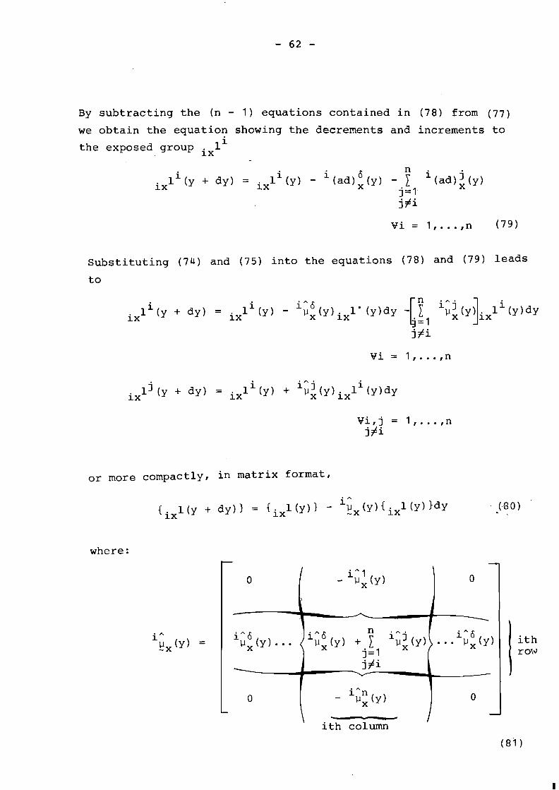
By subtracting the (n - 1) equations contained in (78) from (77)
we obtain the equation showing the decrements and increments to i
the exposed group ixl
Substituting (74) and (75) into the equations (78) and (79) leads
to
j iAj 1 (y + dy) = ix l l (~) + P ~ ( Y ) ~ ~ ix li (y)dy
or more compactly, in matrix format,
i " . 1x l(y + dy)} = {ixl(y)} - tf,(~){~,l(Y)}d~
where:
ith column
(81 1
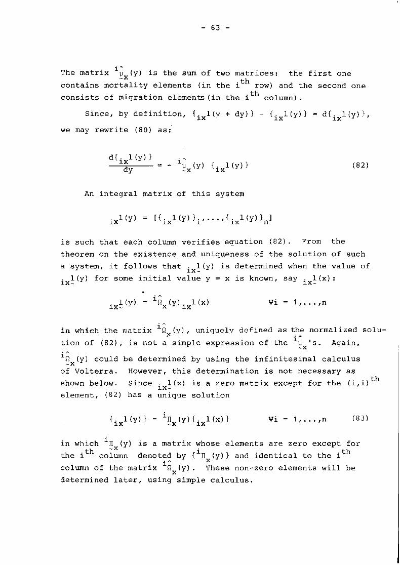
1 The matrix yx(y) is the sum of two matrices: the first one
contains mortality elements (in the ith row) and the second one
consists of migration elements (in the ith column).
Since, by definition, {ixl(v + dy)} - {ixl(y)l = d{ixl(y)),
we may rewrite (80) as:
An integral matrix of this system
is such that each column verifies equation (82). Prom the
theorem on the existence and uniqueness of the solution of such
a system, it follows that ixt(y) is determined when the value of
1 (x) : l(y) for some initial value y = x is known, say ix_ ix-
i A 1 (y) = Rx(y) ixl (x) ix-
i" in which the matrix Rx(y) , uniquely defined as the normalized solu-
tion of (82), is not a simple expression of the i" yx 's. Again,
i" R (y) could be determined by using the infinitesimal calculus -X
of Volterra. However, this determination is not necessary as
shown below. Since l(x) is a zero matrix except for the (i,i) th ix-
element, ( 8 2 ) has a unique solution
i in which nTr(y) is a matrix whose elements are zero except for - A
the ith column denoted by {iilx(y) 1 and identical to the i th . A
I column of the matrix Rx(y). These non-zero elements will be
determined later, using simple calculus.
Because of the following identity:
we have:
(83) can also be rewritten in matrix form as
and xlx is adiagonal matrix allocatinq the survivors of 16 at age
X.
iAj Clearly, the probability vx that an individual present at
age x in state i will survive in state j, T years later,is the
(j,i) th element of the matrix @ = n (x + T). -X --X
In contrast to the movement case, we can express the elements
of fix as functions of the forces of mortality and mobility using
simple calculus. Equation (77) can be rewritten as:
whose integral solution is:
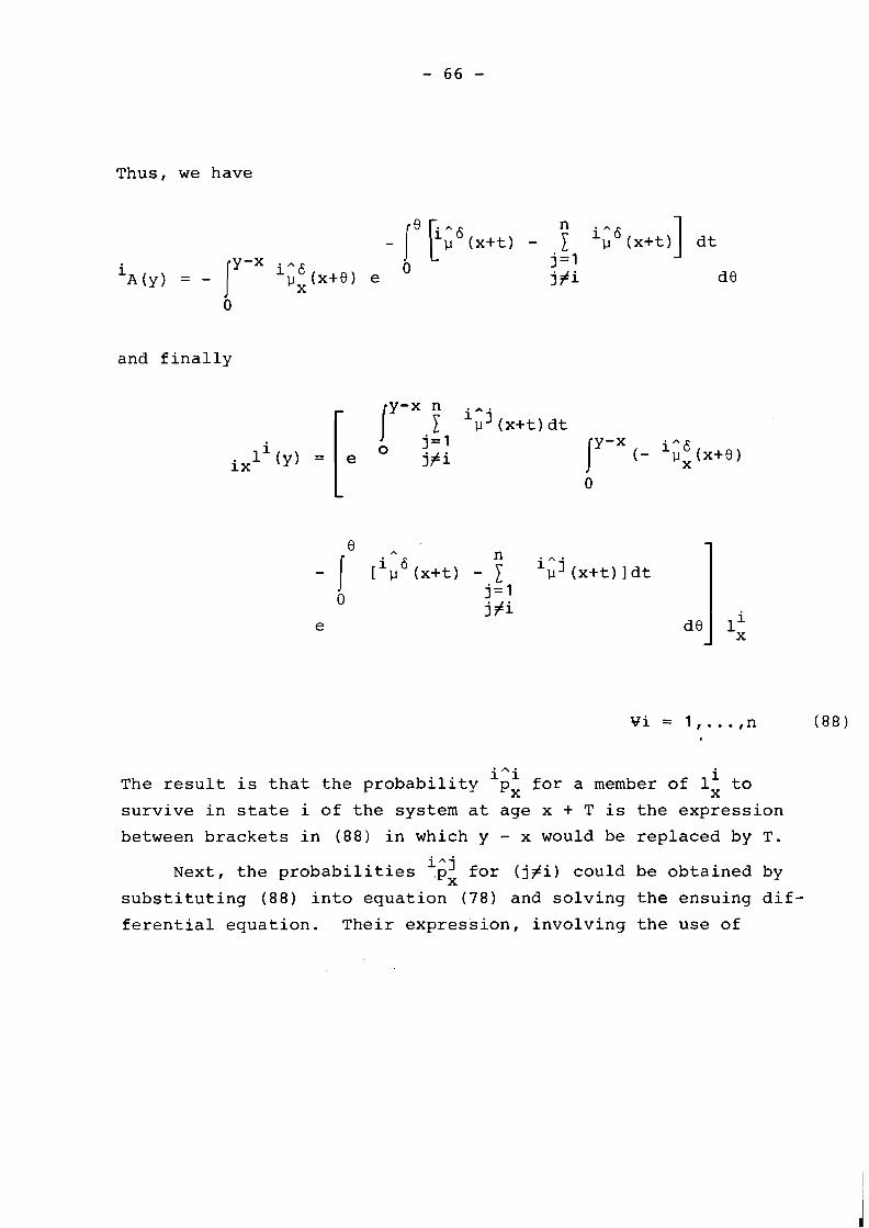
Thus, we have
and finally
y-x n iAj
0 j=1
ix j#i 0
A .
i 6 n iA j u (x+t) ldt
0 j=1 j#i
e de 1 i"i The result is that the probability px for a member of li to
X survive in state i of the system at age x + T is the expression
between brackets in (88) in which y - x would be replaced by T.
Next, the probabilities iAj for (j+i) could be obtained by 'Px substituting (88) into equation (78) and solving the ensuing dif-
ferential equation. Their expression, involving the use of
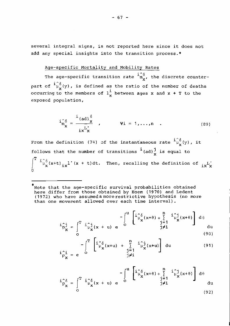
several integral signs, is not reported here since it does not
add any special insights into the transition process.*
Age-specific Mortality and Mobility Rates
The age-specif ic transition rate in6 the discrete counter- x ' iA6 part of px(y), is defined as the ratio of the number of deaths
occurringto the members of 1; between ages x and x + T to the
exposed population,
iA6 From the definition (74) sf the instantaneous rate px (y) , it i follows that the number of transitions (ad)' is equal to
X
Then, recalling the definition of
* Note that the age-specific survival probabilities obtained here differ from those obtained by Hoem (1970) and Ledent ( 1972) who have assumeda more restrictive hypothesis (no more than one movement allowed over each time interval) .
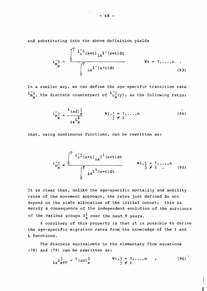
and substituting into the above definition yields
In a similar way, we can define the age-specific transition rate
iA j ikJ the discrete counterpart of px(y), as the following ratio: x'
that, using continuous functions, can be rewritten as:
It is clear that, unlike the age-specific mortality and mobility
rates of the movement approach, the rates just defined do not
depend on the state allocation of the initial cohort: this is
merely a consequence of the independent evolution of the survivors
of the various groups 1; over the next T years.
A corollary of this property is that it is possible to derive
the age-specific migration rates from the knowledge of the 1 and
L functions.
The discrete equivalents to the elementary flow equations
(78) and (79) can be rewritten as:
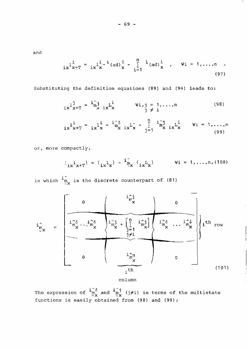
and
S u b s t i t u t i n g t h e d e f i n i t i o n e q u a t i o n s ( 8 9 ) a n d (94 ) l e a d s t o :
o r , more c o m p a c t l y ,
i A
i n which m i s t h e d i s c r e t e c o u n t e r p a r t o f ( 8 1 ) -X
column
ith row
The e x p r e s s i o n o f ii: and i A j mx ( j # i ) i n t e r m s o f t h e m u l t i s t a t e
f u n c t i o n s i s e a s i l y o b t a i n e d f rom ( 9 8 ) a n d ( 9 9 ) :
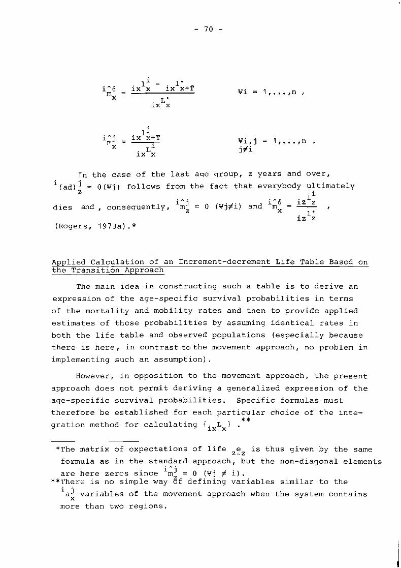
In the case of the last age qroup, z years and over, i (ad): = O(Uj) follows from the fact that everybody ultimately
iAd - iz'z dies and, consequently, iii = 0 (Yj#i) and rn x - - , Z 1'
iz z (Rogers, 1973a).*
Applied Calculation of an Increment-decrement Life Table Based on the Transition Amroach
The main idea in.constructing such a table is to derive an
expression of the age-specific survival probabilities in terms
of the mortality and mobility rates and then to provide applied
estimates of these probabilities by assuming identical rates in
both the life table and observed populations (especially because
there is here, in contrastta~the movement approach, no problem in
implementing such an assumption).
However, in opposition to the movement approach, the present
approach does not permit deriving a generalized expression of the
age-specific survival probabilities. Specific formulas must
therefore be established for each particular choice of the inte- * * gration method for calculating lixLx} .
*The matrix of expectations of life z" is thus given by the same
formula as in the standard approach, but the non-diagonal elements iA j -
are here zercs since m~ - 0 (Vj # i). **There is no simple way of defining variables similar to the
iaJ variables of the movement approach when the system contains X
more than two regions.
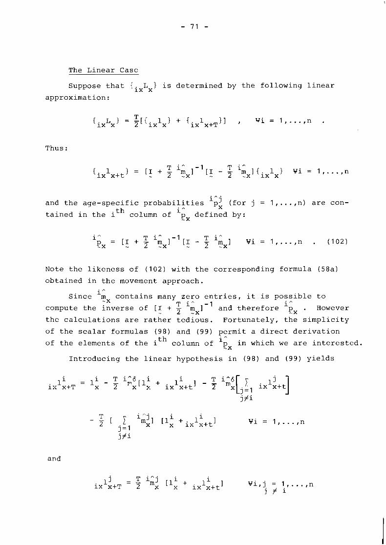
The Linear Case
Suppose that liXLx) is determined by the following linear
approximation:
Thus :
iA j and the age-specific probabilities px (for j = 1, ..., n) are con-
tained in the ith column of i n Px defined by:
Note the likeness of (102) with the corresponding formula (58a)
obtained in the movement approach. . A I Since m contains many zero entries, it is possible to
-X T iA - 1 i A compute the inverse of [I + - m I and therefore px . However - 2 -x the calculations are rather tedious. Fortunately, the simplicity
of the scalar formulas (98) and (99) permit a direct derivatian
of the elements of the ith column of in which we are interested. Px
Introducing the linear hypothesis in (98) and (99) yields
and
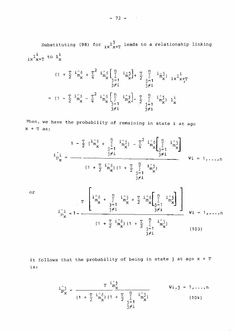
Substituting ( 9 8 ) for ixli+T leads t o a relationship linking
Then, we have the probability of remaining in state i at age
x + T as:
It fol lows that the probability of being in state j at age x + T
is:
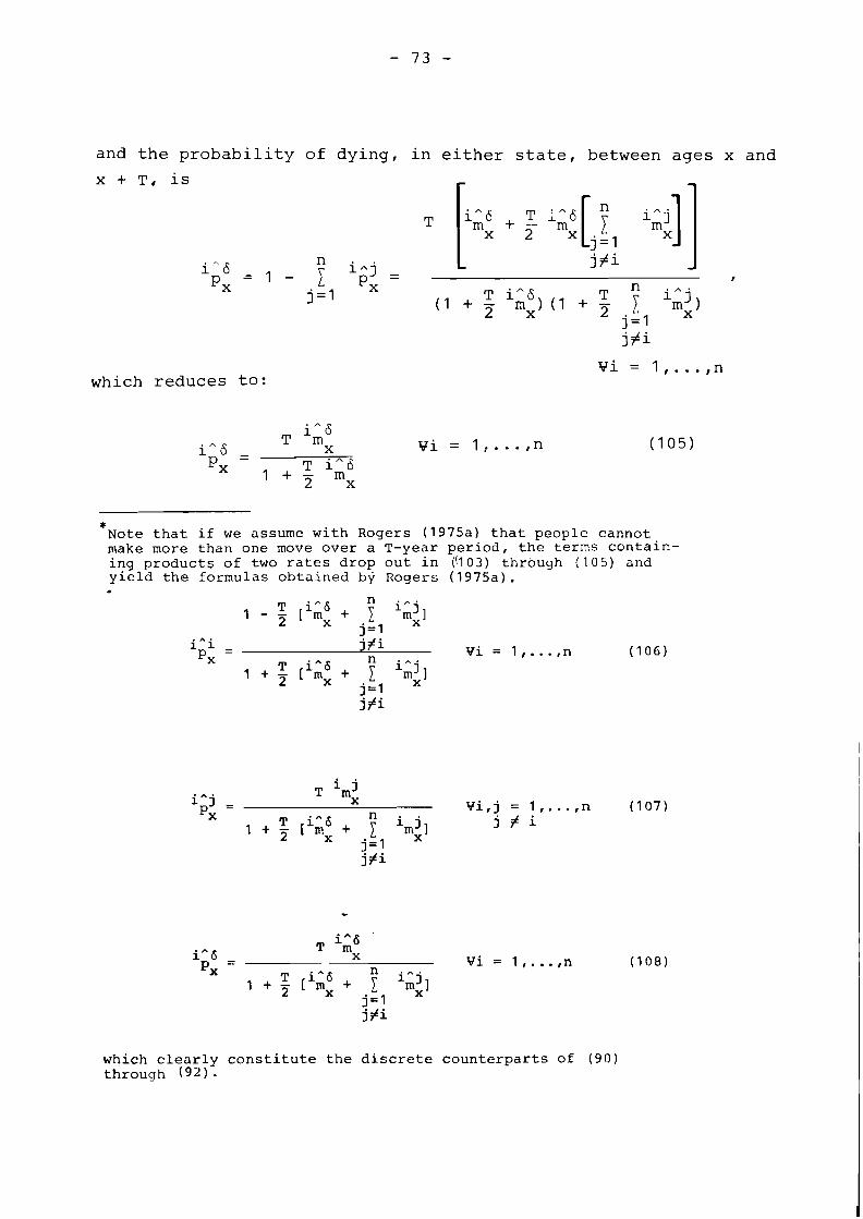
and the probability of dying, in either state, between ages x and
Vi = 1, ..., n which reduces to:
* Note that if we assume with Rogers (1975a) that people cannot make more than one move over a T-year period, the terms contair- ing products of two rates drop out in ((103) through (105) and yield the formulas obtained by Rogers (1975a).
which clearly constitute the discrete counterparts of (90) through (92) .
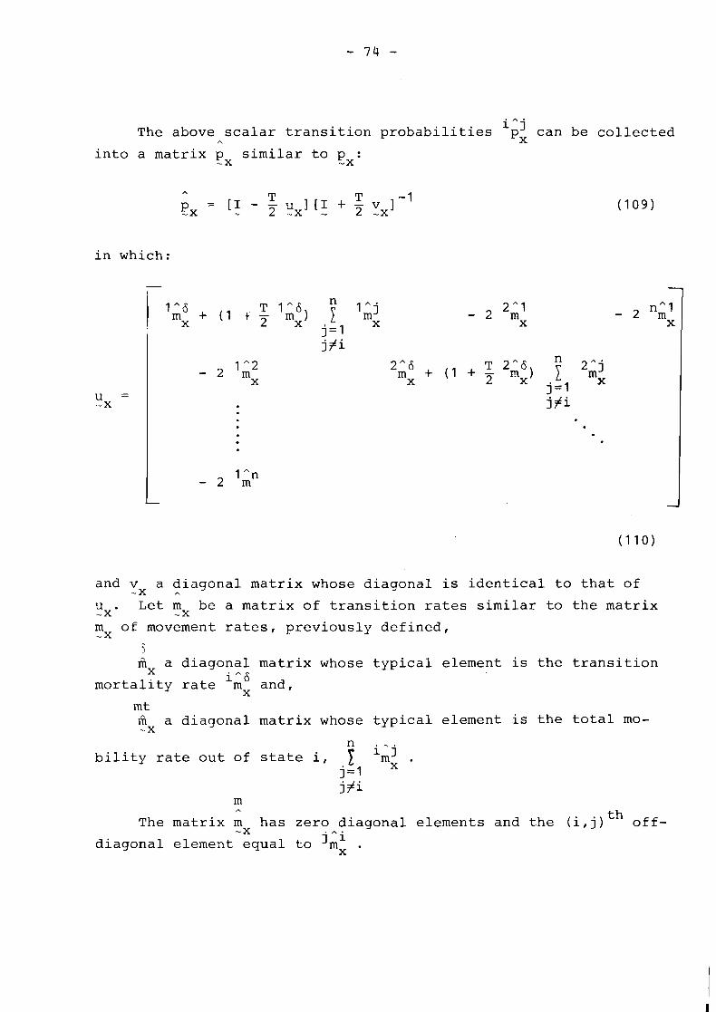
i A j The above scalar transition probabilities
A px can be collected
into a matrix p similar to p : -X -X
in which:
and vx a diagonal matrix whose diagonal is identical to that of - A
u . Let mx be a matrix of transition rates similar to the matrix -x - m of movement rates, previously defined, -x
$3 A a diagonal matrix whose typical element is the transition
X iA6 mortality rate mx and,
mt m a diagonal matrix whose typical element is the total mo- -X
n iA j bility rate out of state i, m .
j = 1 X
h
The matrix m has zero diagonal elements and the (if j ) th off- -X j "i diagonal element equal to mx .
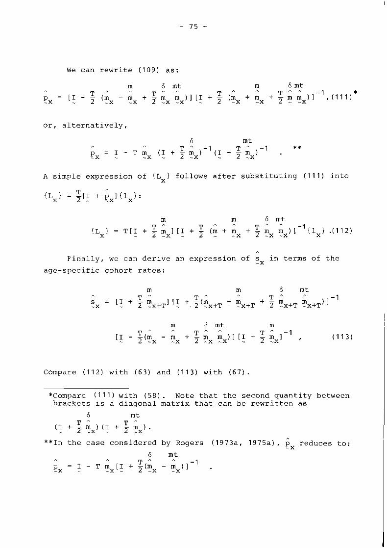
We can rewrite (109) as:
or, alternatively,
A simple expression of {Lx] follows after substituting (111) into
A
Finally, we can derive an expression of s in terms of the -x age-specific cohort rates:
Compare (112) with (63) and (113) with (67).
*Compare (111) with (58). Note that the second quantity between brackets is a diagonal matrix that can be rewritten as
A
**In the case considered by Rogers (1973a, 1975a), px reduces to:
A
6 mt A T A
A -1 - = I - ~ m [ I + - ( m - m ) 1 rx - -x - 2 - x -x
Substituting observed life table rates into (109) provides
estimates of the age-specific survival probabilities from which
all other multistate functions can then be derived. In the case
of the last age group, (100) becomes:
i" in which m is a zero matrix except for the ith row whose elements - z
i" j are all equal to im: (since m = 0 Vj + i). z
This last vector equality actually reduces to a unique scalar
equation
which is insufficient to determine L' for all j = 1 , . . . ,n. Thus, iz z
the general assumptions embodied in this transition approach do
not permit us to determine, from the availability of the transi-
tion mortality rates, the various numbers of person-years lived * in each state.
Consequently, only the movement approach allows for an exact
calculation of the multistate life table functions of the last
group.
Alternative Methods for Deriving EL^)
In opposition to the movement approach, the transition ap-
proach cannot use the cubic integration method which requires
the simultaneous consideration of different age groups. However,
an interpolative-iterative is possible. Such a method adapting
the general procedure developed by Oechsli (1972, 1975) to the
*Because he supposes that no more than one move is made within each age interval (including the last one), Rogers (1973a, 1975a) has
iAB Li ~j = 0 (Vj + i) and 1; = m~ iz z ix z
transition approach was set forth in Ledent (1972) and Ledent/Roqers
(1972). Actually, it does not differ much from the method pro-
posed in the movement approach (see Section 11).
The main difference is that the multistate stationary pop-
ulation is further broken down into groups characterized by the
state of presence at the beginning of the period and that the
separate consideration of these groups makes it possible to "do
away" with the radix problem.
The method used in the movement approach remains valid here, * with vectors replacing matrices , but the age-specific life table
rates for the consolidated intervals are now obtained from:
and
instead of (72).
*The use of the interpolative-iterative methodology in the tran- sition approach is equivalent to its use in the movement approach for a system with a single radix.
IV. MOVEMENT APPROACH VERSUS TRANSITION APPROACH: A FINAL THEORETICAL ASSESSMENT
The purpose of this section is to compare the respective
merits of the two alternative approaches to the construction of
increment-decrement life tables, and thus to shed some light on
the controversy that has been going on between Schoen (1975, 1977)
and Rogers/Ledent (1 976, 1977) .
Nature of the Two A ~ ~ r o a c h e s Contrasted
In both approaches the discrete age distribution {lx} is ob-
tained by the application of a series of transition matrices to
an initial cohort (1 1. However, these matrices are estimated 0
differently owing to the distinct focus of both approaches. To
be more specific, when estimating the probability of an individual
moving out of a state i over a fixed period of time, (1) the
movement approach takes into account all of the moves made by
the individual over that one period of time (whether state i is
involved or not) while, (2) the transition approach compares the
individual's state of presence at the beginning and end of that
period, i.e., at two given points in time.
Consider a group of individuals present at age x in state i.
The transition approach focuses on the net balance of moves from
state i to state j made by the members of this group between ages
x and x + T. On the other hand, the movement approach follows
all the moves made by these individuals over the same T-year period,
thus explicitly considering all gross flows of moves between each
pair of states k,j = l,...,n). The information needed in the * transition approach is somewhat less than in the movement approach,
and may be considered as a "reduced form" of the movement approach.
Further insights can be made by comparing the continuous pat-
terns of mortality and mobility that underline each approach.
*From an applied point of view, the information sought in the transition approach is also easier to collect, which explains why migration data are generally available in terms of transitions rather than moves.
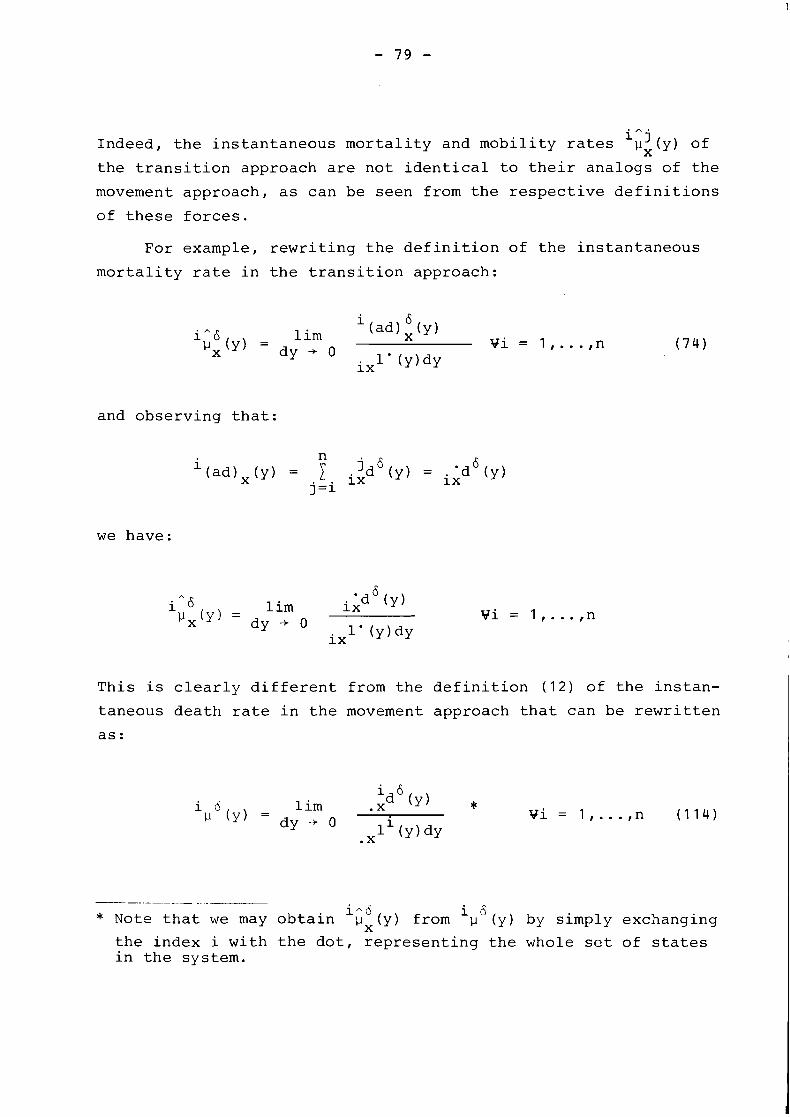
iAj Indeed, the instantaneous mortality and mobility rates px(y) of
the transition approach are not identical to their analogs of the
movement approach, as can be seen from the respective definitions
of these forces.
For example, rewriting the definition of the instantaneous
mortality rate in the transition approach:
and observing that:
we have :
This is clearly different from the definition (12) of the instan-
taneous death rate in the movement approach that can be rewritten
as:
-- - . - -- -. - . . i ~ 6 i 6 * Note that we may obtain ux(y) from p (y) by simply exchanging
the index i with the dot, representing the whole set of states in the system.
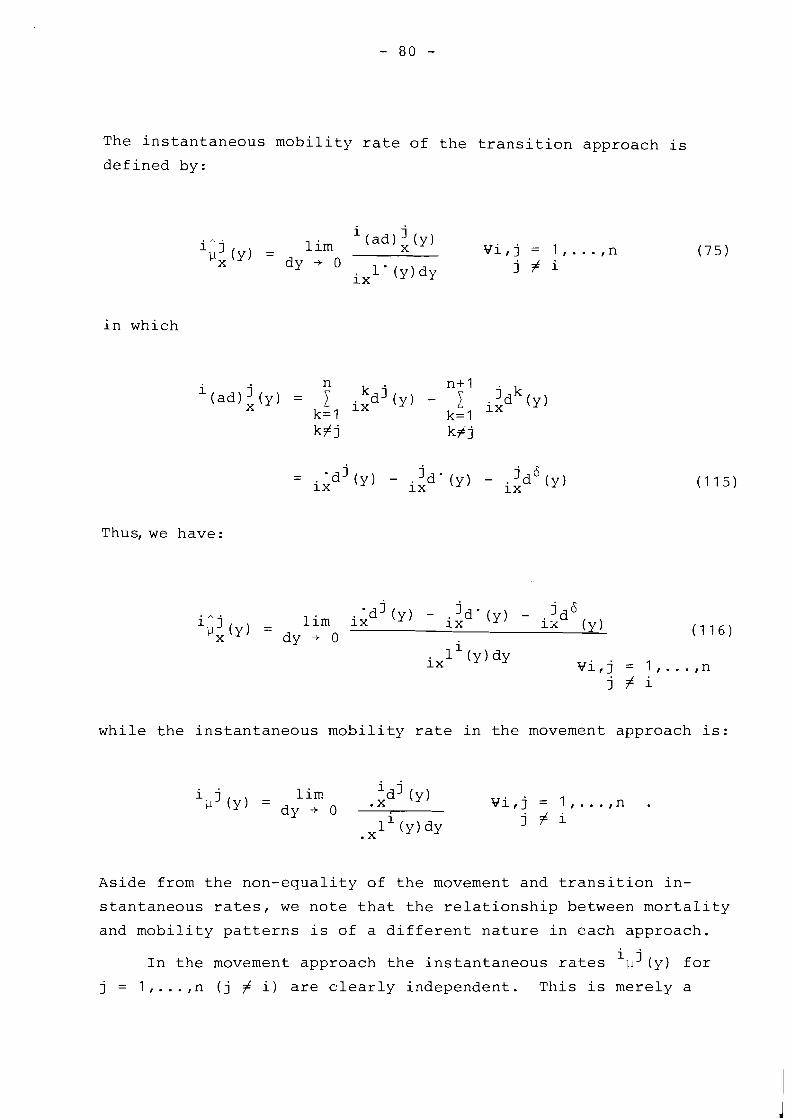
The instantaneous mobility rate of the transition approach is
defined by:
in which
i j n k j
n+ 1 (ad)x(y) = ixd (y)
k= 1 k=l Idk (y) - ix
j = d (y) - d ( ) - ix ix
Thus, we have:
while the instantaneous mobility rate in the movement approach is:
Aside from the non-equality of the movement and transition in-
stantaneous rates, we note that the relationship between mortality
and mobility patterns is of a different nature in each approach.
i j In the movement approach the instantaneous rates y (y) for
J = l,...,n j # i are clearly independent. This is merely a
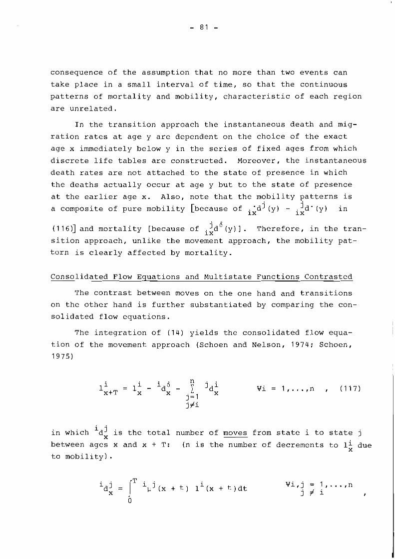
consequence of the assumption that no more than two events can
take place in a small interval of time, so that the continuous
patterns of mortality and mobility, characteristic of each region
are unrelated.
In the transition approach the instantaneous death and mig-
ration rates at age y are dependent on the choice of the exact
age x immediately below y in the series of fixed ages from which
discrete life tables are constructed. Moreover, the instantaneous
death rates are not attached to the state of presence in which
the deaths actually occur at age y but to the state of presence
at the earlier age x. Also, note that the mobility patterns is
- jdS(y) in a composite of pure mobility [because of i;dl (y) ix
( 1 1 ti)] and mortality [because of jds (y) 1 . Therefore, in the tran- ix
sition approach, unlike the movement approach, the mobility pat-
tern is clearly affected by mortality.
Consolidated Flow Equations and Multistate Functions Contrasted
The contrast between moves on the one hand and transitions
on the other hand is further substantiated by comparing the con-
solidated flow equations.
The integration of (14) yields the consolidated flow equa-
tion of the movement approach (Schoen and Nelson, 1974; Schoen,
1975)
i j in which d is the total number of moves from state i to state j
X between ages x and x + T: (n is the number of decrements to li due
X to mobility) .
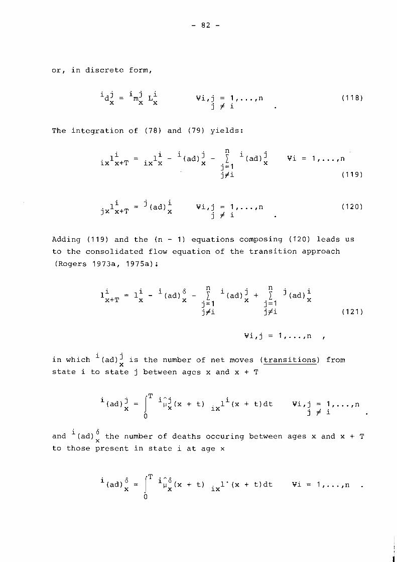
or, in discrete form,
The integration of (78) and (79) yields:
li i = j (ad) Vi,j = l,...,n jx x+T
j f i
Adding (1 19) and the (n - 1 ) equations composing (1 20) leads us
to the consolidated flow equation of the transition approach
(Rogers 1973a, 1975a) ;
i in which (ad) is the number of net moves (transitions) from X
state i to state j between ages x and x + T
i and (ad): the number of deaths occuring between ages x and x + T
to those present in state i at age x

i In discrete form, the net decrements to lx are respectively: -
. A .
i (ad)' = 'm' Li Vi,] = 1 ,. .. ,n x x ix x J f i I
and
i iA6 L. (ad): = m X ix x
An important aspect of the comparison between the two alter-
native approaches is that (121) of the transition approach can be
broken down into n separate equations [contained in (119) and (120)l
while (117) of the movement approach cannot.
The substitution of the net decrements into the flow equations 2
of the transition approach lead to n scalar equations, summarized
as
while substitution of gross decrements into the flow equation of
the movement approach yields only n scalar equations, summarized
as :
Consequently, from the knowledge of multistate functions,
(122), unlike (123),allows for the derivation of life table rates,
which permits the elimination of the radix problem without imposing
any further assumptions. In the movement approach however, a
further assumption (independence of the life table rates from the
state allocation of the initial cohort) must be introduced. Ac-
tually it is equivalent to suppose that (117) holds for each group
li rather than for 1; = li alone. jy x .Y x
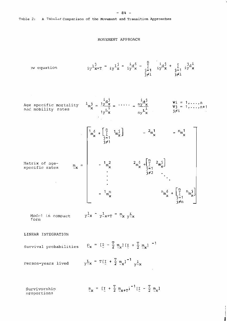
- 8 4 - Table 2: A Tabular Comparison of the Movement and Transition Approaches
MOVEMENT APPROACH
2w equation
i j d i j d
Age specific mortality imJ = - - 'y - - . . . - - - - nY x a112 mobility rates x L~
I Y x L~
nY x
Matrix of age- specific rates
Modc! in compact f orn
LINEAR IXTEGRATION
T T = [ I - - m 1 [ 1 + - m ] - 1
Survival probabilities ex - 2 -x - 2 -x
T L = T [ I + - m ] - 1 Ferson-years lived Y-X - 2 -x 1 Y-x
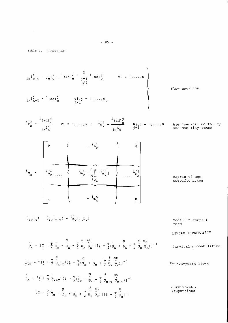
T a b l e 2 . ( c o n t i n u e d )
Flow e q u a t i o n
i j ( a d )
mx - - ~i = l , . . . , n ; = - j = l t n A3c ' ; p e c i f i c r ? o r t a l i t y L' X
i x x L~ j # l and m o b i l i t y r a t e s i x x
pla,tr ix of age- s u e c i f i c r a t e s
Model i n compact form
LIYEAR INTEGRATION
m 6 m t 6 m t A T A A T A " T " T? T . " " - 1 px = [ I - ~ ( m - m + - m mx)-III + ? (mx + m x + ? m x E ~ ) ] - . x x 2 - x S u r v i v a l p r o b a b i l i t i e s
P e r s o n - y e a r s l i v e d
S u r v i v o r s h i p p r o p o r t i o n s
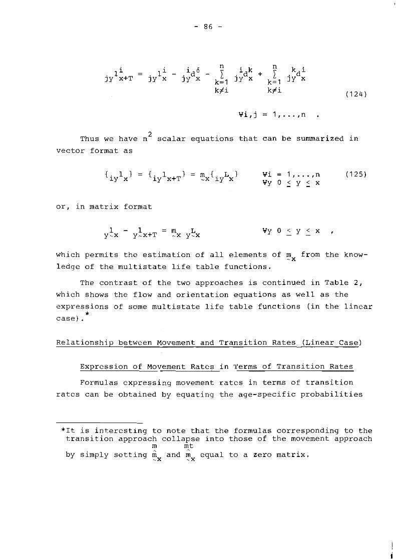
kfi kfi
2 Thus we have n scalar equations that can be summarized in
vector format as
or, in matrix format
which permits the estimation of all elements of mx from the know- - ledge of the multistate life table functions.
The contrast of the two approaches is continued in Table 2,
which shows the flow and orientation equations as well as the
expressions of some multistate life table functions (in the linear * case).
relations hi^ between Movement and Transition Rates (Linear Case)
Expression of Movement Rates in 'llerms of Transition Rates
Formulas expressing movement rates in terms of transition
rates can be obtained by equating the age-specific probabilities
*It is interesting to note that the formulas corresponding to the transition approach collapse into those of the movement approach
m nt A
by simply setting I?I and m equal to a zero matrix. -X - X
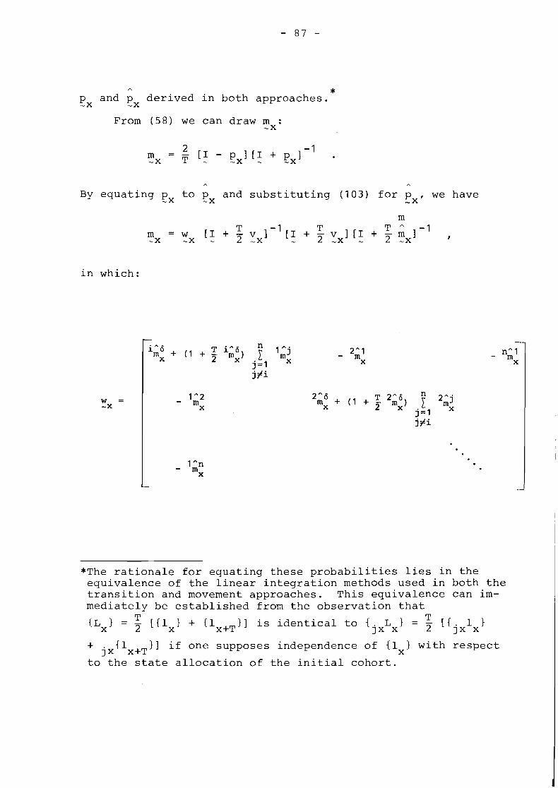
A * Px and p derived in both approaches. -x
From (58) we can draw mx:
A A
By equating p to px and substituting ( 1 0 3 ) for px, we have -.x - -
in which:
*The rationale for equating these probabilities lies in the equivalence of the linear integration methods used in both the transition and movement approaches. This equivalence can im- mediately be established from the observation that
T T { L ~ ) = 2 [{l 1 + {I 11 is identical to ljXLX) = [ { 1 ) x x+T jx x
+ jxtlx+T 11 if one supposes independence of 11 1 with respect X
to the state allocation of the initial cohort.
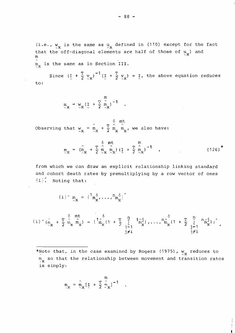
(i.e., w is the same as F~ defined in (1 10) except for the fact -X
that the off-diagonal elements are half of those of u ) and -X m
A
n is the same as in Section 111. -x
T -1 T Since (I + yX) (I + - v ) = I I the above equation reduces - - 2 7X -
A
6 mt T A A
Observing that wx = m + - m m we also have: - -X 2 x x 1
from which we can draw an explicit relationship linking standard
and cohort death rates by premultiplying by a row vector of ones
{i): Noting that:
*Note that, in the case examined by Rogers (1975), w reduces to I\. -x m so that the relationship between movement and transition rates -- X is simply:
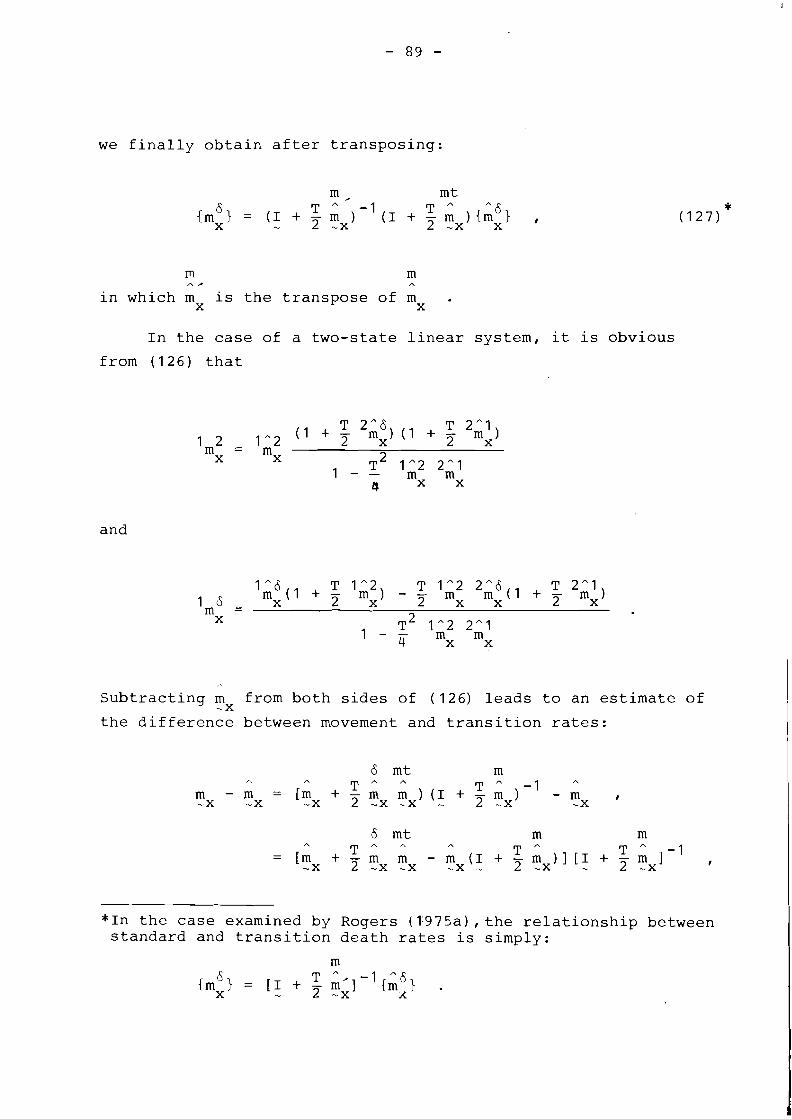
we finally obtain after transposing:
in which m is the transpose of m .. X X
In the case of a two-state linear system, it is obvious
from (126) that
and
Subtracting m from both sides of (126) leads to an estimate of -X
the difference between movement and transition rates:
*In the case examined by Rogers (1:975a),the relationship between standard and transition death rates is simply:
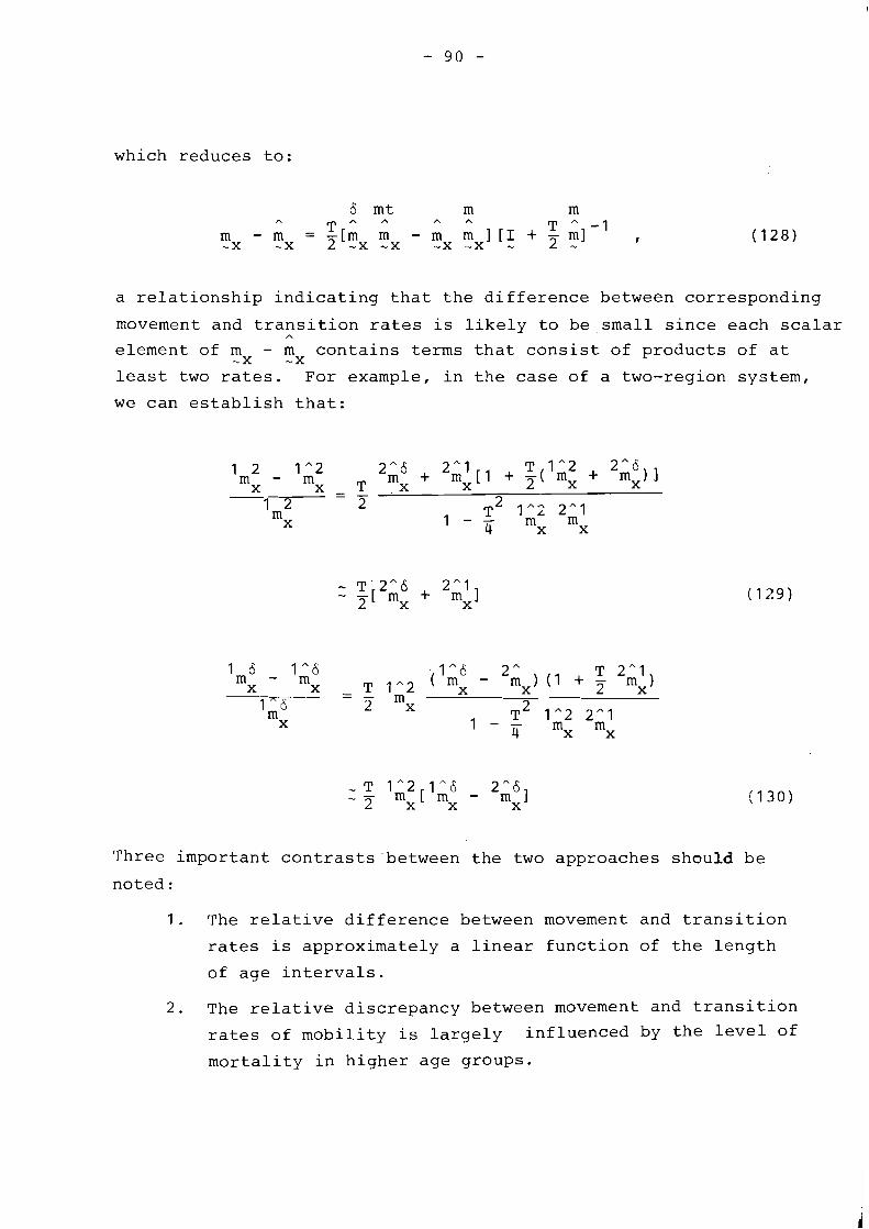
which reduces to:
a relationship indicating that the difference between corresponding
movement and transition rates is likely to be small since each scalar A
element of mx - m contains terms that consist of products of at - -X
least two rates. For example, in the case of a two-region system,
we can establish that:
1 6 I A 6 A
m - m T 2 " 1 X
IA6 - 2m ) ( I + 7 mx) X - - T - l A 2 ( x x m "2 2 x
X T~ I A 2 2 ^ 1
1 - mx mx
Three important contrasts-between the two approaches should be
noted:
1 . The relative difference between movement and transition
rates is approximately a linear function of the length
of age intervals.
2 . The relative discrepancy between movement and transition
rates of mobility is largely influenced by the level of
mortality in higher age groups.
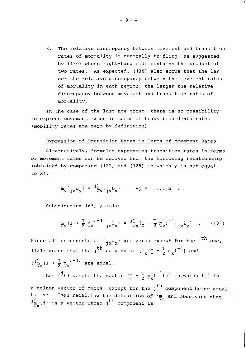
3. The relative discrepancy between movement and transition
rates of mortality is generally trifling, as suggested
by (130) whose right-hand side contains the product of
two rates. As expected, (130) also snows that the lar-
ger the relative discrepancy between the movement rates
of mortality in each region, the larger the relative
discrepancy between movement and transition rates of
mortality.
In the case of the last age group, there is no possibility
to express movement rates in terms of transition death rates
(mobility rates are zero by definition) .
Expression of Transition Rates in Terms of Movement Rates
Alternatively, formulas expressing transition rates in terms
of movement rates can be derived from the following relationship
(obtainkd by comparing (122) and (125) in which y is set equal
to x) :
Substituting (63) yields:
th Since all components of {jxlx} are zeros except for the j one,
T (1 31 ) means that the jth columns of [m (I + - m ) 1 and x - 2 -x
T - 1 (I + - m ) 1 are equal. -x - 2 -x
T Let {jh} denote the vector (I + - rn j~ in which { j 1 is - 2 -x
a column vector of zeros, except for the jth component being equal A
to one. Then recalling the definition of jm and observing that A -X
jm { j 1 is a vector whose jth component is -x
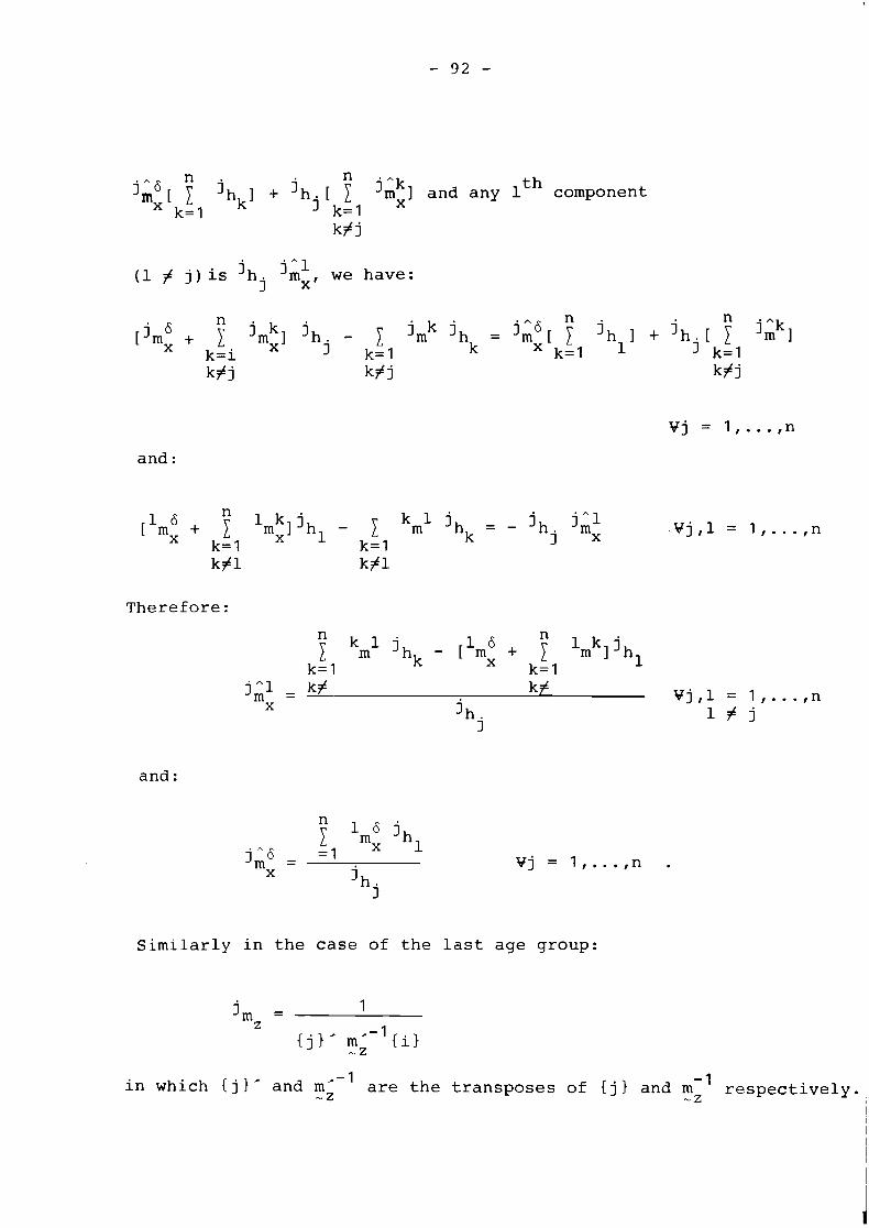
n n jA6 mx [ 1 jhk] + jh [ 1 jm;] and any lth component k= 1 k= 1
jA1 wehave: (1 # j) is hj m x f
and :
Therefore:
k l j n 1 m h k - [ m
l k j 1 6 + 1 m ] h l
k= 1 X k= 1
and :
Similarly in the case of the last age group:
in which { j and mO-' are the transposes of { j 1 and m-' respectively. - z - Z
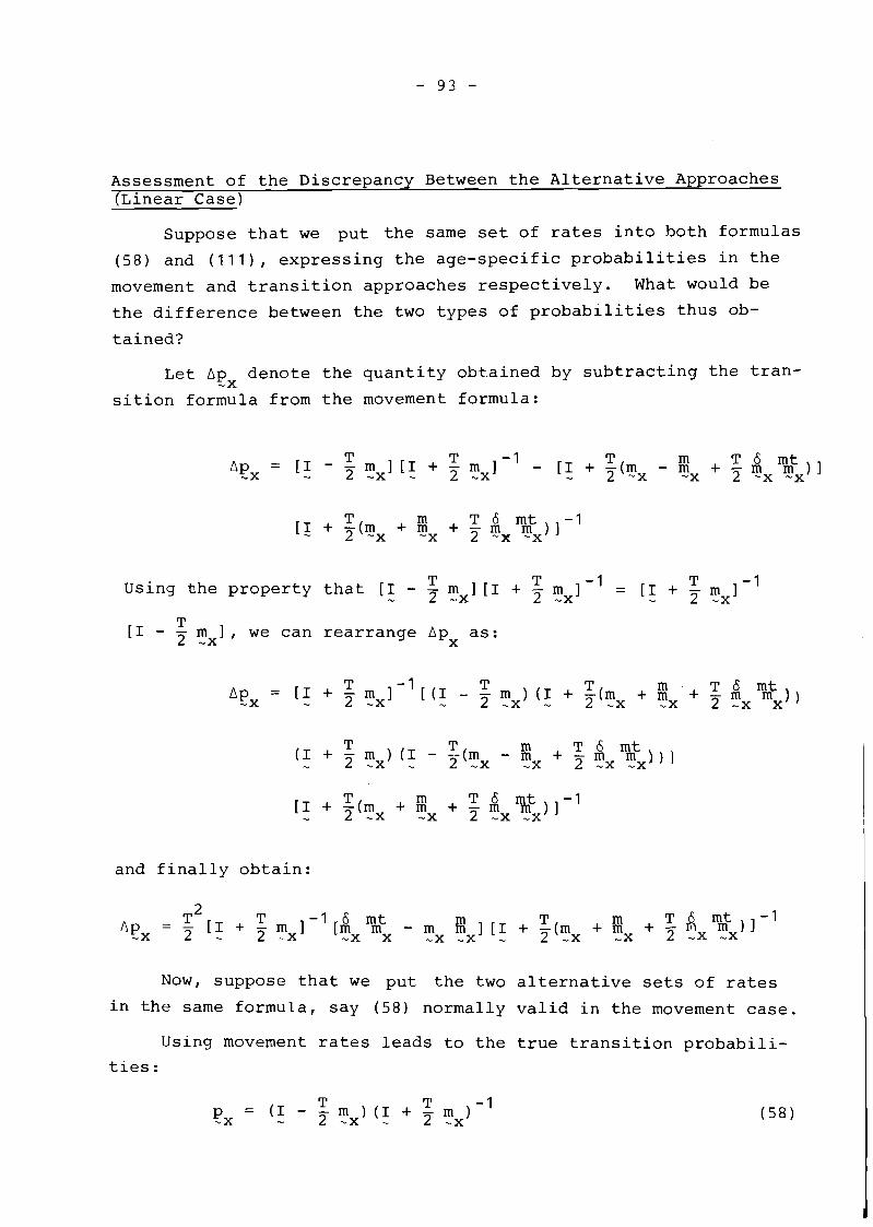
Assessment of the Discrepancy Between the Alternative Approaches (Linear Case)
Suppose that we put the same set of rates into both formulas
(58) and (Ill), expressing the age-specific probabilities in the
movement and transition approaches respectively. What would be
the difference between the two types of probabilities thus ob-
tained?
Let Apx denote the quantity obtained by subtracting the tran-
sition formula from the movement formula:
T T -1 T Using Ohe property that [I - - m ][I + - m 1 = [I + - m ] - 1 - 2 -X 2 -x - 2 -x
T [I - - m I, we can rearrange Ap as: 2 --X X
T - 1 T T m T 6 mt = [I + - m I [(I - - m )(I + -(m - 2 -x + - m m ) ) - 2 - x - 2 - x + " 2 - x x
and finally obtain:
Now, suppose that we put the two alternative sets of rates
in the same formula, say (58) normally valid in the movement case.
Using movement rates leads to the true transition probabili-
ties :
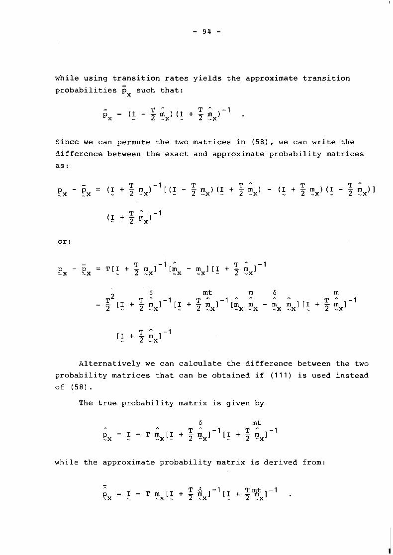
while using transition rates yields the approximate transition
probabilities px such that:
Since we can permute the two matrices in (58), we can write the
difference between the exact and approximate probability matrices
as :
- - T - 1 T A T T A
= (I + - m ) [(I - 5mx)(I + Trnx) - (I + - m )(I - - m )I Px Px - 2 -x - - - 2 -x - 2 -x
or:
Alternatively we can calculate the difference between the two
probability matrices that can be obtained if (111) is used instead
of (58) . The true probability matrix is given by
while the approximate probability matrix is derived from:
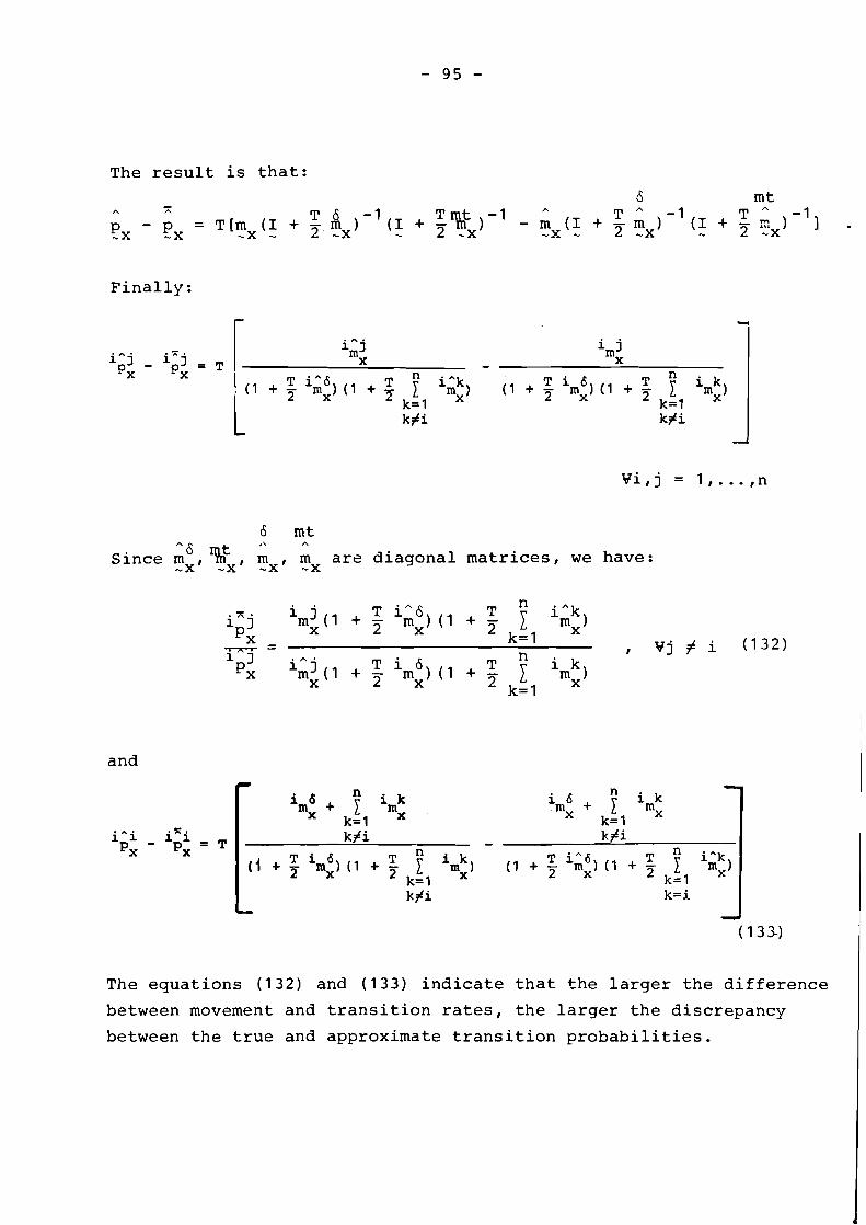
The result is that:
Finally:
h
6 mt r\ h
Since m:, % , m , rn are diagonal matrices, we have: - -X -X -X
and
The equations (132) and (133) indicate that the larger the difference
between movement and transition rates, the larger the discrepancy
between the true and approximate transition probabilities.
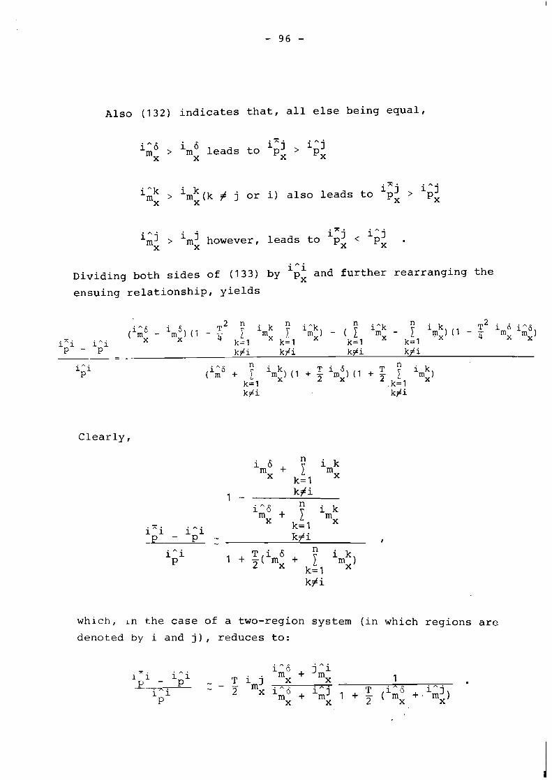
Also (132) indicates that, all else being equal,
- iAj > iA j ik6 > im6 leads to px X X px
iAk mx X
> iA j > imk (k # j or i) also leads to px px
iXj < iA j ikJ > imj however, leads to px X X px
iAi Dividing both sides of (133) by px and further rearranging the
ensuing relationship, yields
Clearly,
1 .- - kfi
kfi
which, ~n the case of a two-region system (in which regions are
denoted by i and j), reduces to:
iiS + jA i i x i - iAi m P p - T i j - x X . .~
1 m . -
iAi iAj P - 2 x iA6 x + imj x + 5 (iks x + mx)
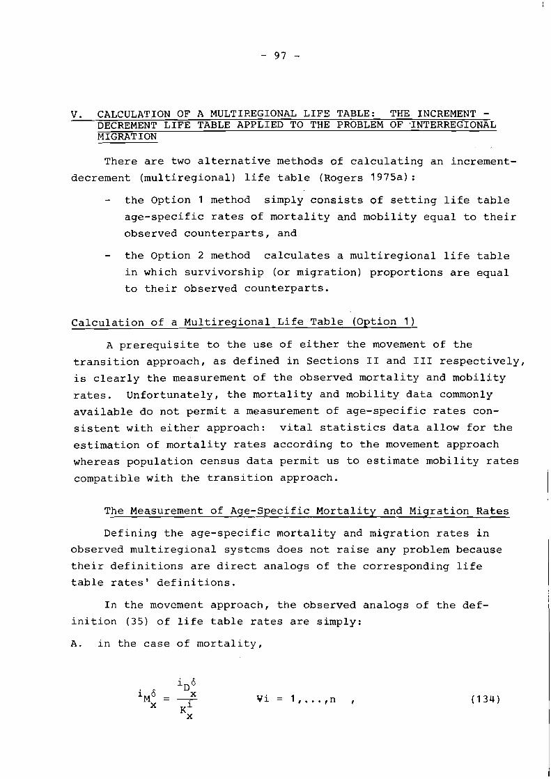
V. CALCULATION OF A MULTIREGIONAL LIFX TABLE: THE INCREMENT - DECREMENT LIFE TABLE APPLIED TO THE PROBLEM OF -INTERREGIONAL MIGRATION
There are two alternative methods of calculating an increment-
decrement (multiregional) life table (Rogers 1975a) :
- the Option 1 method simply consists of setting life table
age-specific rates of mortality and mobility equal to their
observed counterparts, and
- the Option 2 method calculates a multiregional life table
in which survivorship (or migration) proportions are equal
to their observed counterparts.
Calculation of a Multiregional Life Table (Option 1)
A prerequisite to the use of either the movement of the
transition approach, as defined in Sections I1 and 111 respectively,
is clearly the measurement of the observed mortality and mobility
rates. Unfortunately, the mortality and mobility data commonly
available do not permit a measurement of age-specific rates con-
sistent with either approach: vital statistics data allow for the
estimation of mortality rates according to the movement approach
whereas population census data permit us to estimate mobility rates
compatibie with the transition approach.
The Measurement of Age-Specific Mortality and Migration Rates
Defining the age-specific mortality and migration rates in
observed multiregional systems does not raise any problem because
their definitions are direct analogs of the corresponding life
table rates' definitions.
In the movement approach, the observed analogs of the def-
inition (35) of life table rates are simply:
A. in the case of mortality,
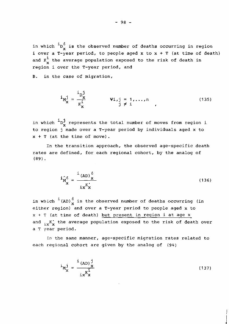
in which iD6 is the observed number of deaths occurring in region X
i over a T-year period, to people aged x to x + T (at time of death)
and K: the average population exposed to the risk of death in
region i over the T-year period, and
B. in the case of migration,
i j in which Dx represents the total number of moves from region i
to region j made over a T-year period by individuals aged x to
x + T (at the time of move).
In the transition approach, the observed age-specific death
rates are defined, for each regional cohort, by the analog of ( 8 9 ) .
i in which (AD): is the observed number of deaths occurring (in
either region) and over a T-year period to people aged x to
x + T (at time of death) but present in region i at age x
and ixK; the average population exposed to the risk of death over
a T year period.
In the same manner, age-specific migration rates related to
each regional cohort are given by the analog of (94)
i (AD) X
P
K' ix x
i in which (AD): is the number of transitions made over a T year
period between regions i and j by people aged x in region i at i
the beginning of the observation period, and ixKx the average
population exposed to the risk of migiating.
Since vital statistics are generally collected by place of
occurrence, estimates of age-specific mortality rates, by region,
consistent with the movement approach can be easily measured by iD6 application of ( 134) : is directly provided by vital statistics
i X
data and Kx can be approximated by the mid-period population of
each age group. In contrast to this, since no link is generally
made, between reporting deaths, the region of death occurrence,
and the region of presence at any earlier age, no age-specific
mortality rates consistent with the transition approach can be
simply measured.
Very few countries have compulsory registration, that makes
it possible to evaluate the total number of moves between pairs
of regions over a given period. In most instances, migration
rates consistent with the movement approach cannot be measured.
Fortunately, a population census generally proves data on place-
to-place migration in terms of reported changes of residence from
a fixed prior date (i.e., viewed as transitions rather than moues)
and thus constitutes a data source consistent with the transition
approach.
Unfortunately, typical migration figures released by most
censuses do not correspond exactly to the numerator of (137). i j Generally, census data reports the number of people Kx (aged
x to x + T at the end of the observed period) present in region
i at the beginning of the period and in region j at the end of i j the period. Therefore, we must approximate to determine (AD)*,
the numerator of ( 1 37) :
i j i j *If x = 0, then KT denotes the number of babies B born in
region i over the T-year period who were present in region j at the end of the period.
We al.so need, to estimate the denominator of (137) which is i
not K: but ixKx . This quantity can be cplculated by a
linear approximation
in which Ki(u) represents the number of people aged y to y + T i , ~ x
in region i at time t and present in the same region u - t years
Ki(t) is nothing more than the population aged x to later. i,x
x + T in region i at the beginning of the period, whereas,
i Ki(t + T) is immediately obtained as K . Also, note the i,x-T x x
existence of further complications for the last age group that
are not reported here.
To summarize, measures of age-specific mortality and migra-
tion rates consistent with either approach generally cannot be
obtained. Most common data only permit us to derive mortality
and migration rates compatible with the movement and transition
approaches respectively. Fortunately, this does not hamper the
applied calculation of a multiregional life table since an alter-
native mixed approach based on the availability of movement death
rates and transition migration rates is possible.
Illustration of Linear and Inter~olative-Iterative Variations
The construction of a multiregional life table from the type
of data generally available can be performed using either the
linear integration method for deriving IL 1 or an interpolative- X
iteration method.
If the linear integration method is retained the relationship
(125) linking the death rates of the movement and transition ap-
proaches can be reformulated as
which provides a simple expression of the death rates (of the
transition approach) in terms of the life table (movement) death
rates and (transition) migration rates.
The age-specific survival probabilities of a multiregional
life table can be expressed in terms of life table (movement) death
rates and (transition) migration rates by substituting (140) into
the formula (1 11) of the transition approach.
The result is, assuming equality of life table and observed
rates, that the age-specific survival probabilities can be ob-
tained from:
6 A
where the diagonal of M is identical to the vector -x
6 in which {M ) is a vector of observed (movement) death rates and
X C i-ii n t 6 r;l A 0 A A h
Mxl Mx and M are the observed counterparts of mx, m m and -X X' X I
m . Thus. initiated by the estlrnatjon of tlie age-specific survival X
!)robabilities, the calculation of Lhe other multistate life table .t= .unctioxs is ~or.plote~ as inai-atoa in c e r t i o n c , TI ?na T T T .
Such a calculation is illustrated using mortality and mig-
ration data for the four region system of the U.S. female pop- * ulation (period of observation 1965-1970). Age-specific (move-
ment) mortality rates for the regions of this system have been
measured by the application of (134) to available data (see the
second column of Movement Rates in Table 6, which provides est-
imates of such mortality rates relating to the third region of the
system: South) while age-specific (transition) migration rates
have been measured by application of (1 37) through (1 39) (the
three columns of Transition Rates in Table 6 providing estimates
of such migration rates out of the third region).
The complete set of probabilities of dying and outmigrating
concerning the South region is given by Survival Probabilities
in Table 3. For instance, a twenty-five year old woman living
in the South has a probability of dying with the next five years
equal to 0.00470. Moreover, her probability of still living in
the South region five years later is equal to 0.92226,while the
probabilities of migrating to the North East, North Central and
West regions are respectively equal to 0.01975, 0.02946 and
0.02383. The two alternative mobility statistics to which the
above transition probabilities lead,expectations of life and net
migraproduction rates, are set out in Table 4. It appears that
a woman born in the South has a life expectancy of 74.30 years,
of which 52.16 can be expected to be spent in the South, 5.73 in
the North East, 8.71 in the North Central and 7.71 in the West.
Alternatively, such a woman is expected to make an average of
0.72 moves out of a U.S. Census region, including 0.52 out of
the South region.
Exact survivorship proportions by place-of-birth for those
residing in the South at age x are displayed in Table 5. The
probability for a woman aged 25 to 30 in the South to survive
*This system is composed of four regions which are precisely the four regions of the United States considered by the U.S. Census Bureau: North East, North Central, South and West.
five years later in the same region is equal to 0.93033 if she
was born in the South. But, for a woman born in other regions
this probability increases to 0.93121 if she was born in the
West. Then, the survivorship proportions for women aged 25 to
30 in the South, independently of their place of residence, stands
somewhere in between 0.93033 and 0.93121. However, the corres-
ponding approximate survivorship proportions calculated from
= L L 'x 0-x+5 0-x is only equal to 0.93017 (as indicated in Table
4), which provides an order of magnitude of the approximation made
by using the aforementioned formula.
Taking advantage of the formulas linking movement and trans-
ition rates (see Section IV), we have calculated the (transition)
death rates and the (movement) migration rates compatible with
the input rates. From the figures in Table 6 we find the follow-
ing two discrepancies:
- transition (mortality) rates are, as expected, only slightly
different from their movement counterparts: slightly
smaller in the young age groups (0.00531 versus 0.00533
for the first age group in the South region), they become
much smaller in the middle age groups and then slightly
higher in the old age groups (0.14948 versus 0.14944 for
the last age group).
- The discrepancy between movement and transition rates of
migration is larger than in the case of mortality. Although,
movement rates are always higher than transition rates, the
discrepancy is relatively small when mortality has little
influence (up to 50 years old) - the migration rate from
South to West in age group 20 to 25 is equal to 0.520 * (movement rate) versus 0.515 (transition rate) - and tends
to augment sharply with age: the movement rate for the
last age group is almost fifty percent higher than the
corresponding transition rate. Indeed, these results were
more or less expected since movement rates of migration,
unlike their transition counterparts, are only slightly
influenced by mortality.
*The discrepancy increases with the intensity of migration.
Table 3. Multiregional life table based on movement death rates and transition rates of migration, linear case, United States, four region system (1965-1970), females, age specific survival probabilities and approxi-
mate survivorship proportions (South Region).
SURVIVAL PROBABILITIES
APPROXIMATE SURVIVORSHIP PROPORTIONS
- 5 f l m 1 1 ~ h h q l h m f l l 1 5 9 7 d . 9 4 3 2 9 r!, 98565 1 6,kl?856 f l .91414
5 4 ( l , k j l l 4 Y d m V q 1 ~ ? 5 9 . 9 5 ~ 9 7 1 , Q , 9 9 7 F q 1 4 , L q l 31- noL!I?15L4 C7,9465U 15 4 , c ) Y h l J c S 4,!4189'4 fl,D399V @,9?hml ? 6' i n . q 3 5 7 U 1 3 M,91 ? L ? , ( ~ C ) / A ? . ~ [ I 1 11,fl2556 d?.Y301 7 7 Cq 3.995'197 1 I r ) , C i l A Q H !3,9/1333 35 T , 3 i i b 2 S I , I A P H A ~ ~ ' , ~ 1 1 3 4 5 E.951 3 4 4 0 r q o & j f l 1 1 1 5 1 h U,\qG74648 Fl,95534 45 ~ > , Y 1 ? 1 h 1 ~ , ~ 9 9 J h v ! ql,d~T1M m.95387 5 (4 h . q h 4 7 h e 1 , v 1 f l 3 7 1 w1,L1G15~2 tAW'3UhRr ) 5 5 p ,YJ47 1 V ) , ~ A ~ I S ? ~ Lo ,WA53R 8 .93197 h ~ ? rT.Y1H5L1 ( A , VIG? 333 [I ,dm512 Mm9G7b36 6 s l O k 7 737 i ? , @ m 457 5 k7.66512 7 M - r ,n1%12 in, l c l h j i 1 , k ? ~ r 1 3 1 M , 79993 75 , 7 1 , 8 .1,k1@4RZ :1,71"35 Rn 1 . ~ r ~ 7 : j n , ! 1 ~ 9 5 1 ~ ~ , U I ~ J I S 1 . 0 ~ ~ 8 2
Table 4. Multiregional life table based on movement death rates and transition rates of migration, linear case, United States, four region system (1965-19701, females, age specific expectations of life and migrapr0- duction rates by place-of-birth (south Region)
EXPECTATIONS OF LIFE
NET MIGRAPRODUCTION RATES
Table 5. Multiregional life table based on movement death rates and transition rates of migration, linear case, United States, four region system (1965-1970), females, exact survivorship proportions by place-of-birth and place-of-residence at age x (South ~egion).
FOR THOSE BORN I N THE NORTH EAST
FOR THOSE BORN I N THE NORTH CENTRAL
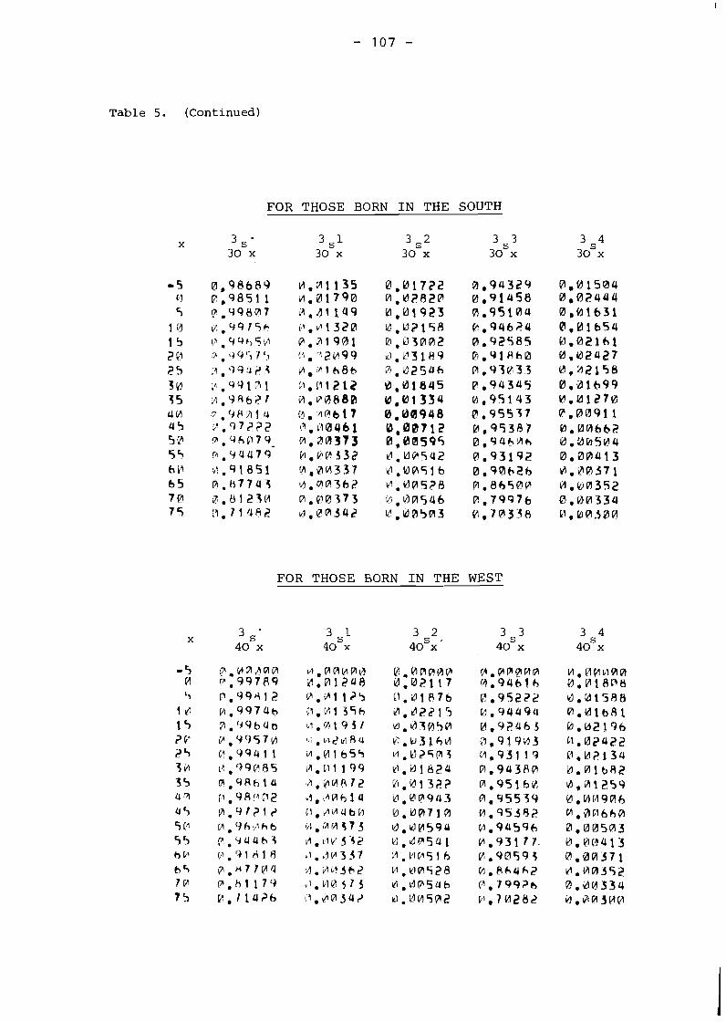
Table 5. (Continued)
F O R THOSE BORN I N T H E SOUTH
F O R T H O S E BORN I N T H E WEST
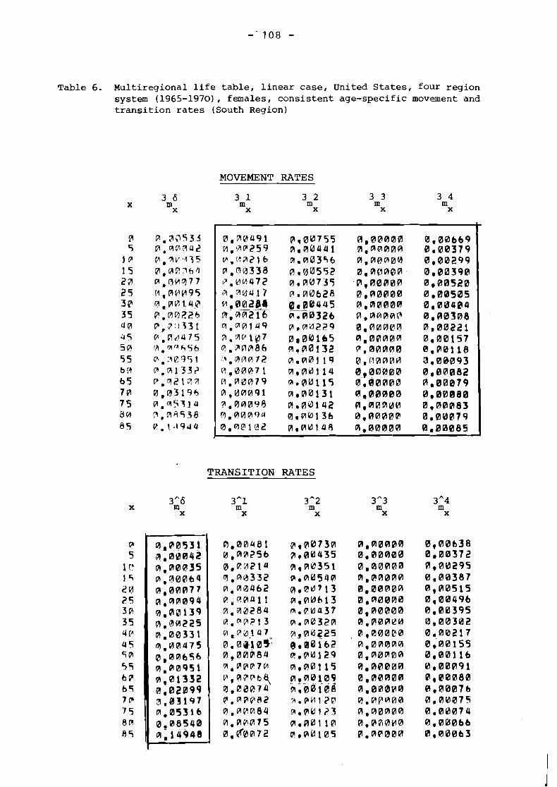
Table 6. Multiregional life table, linear case, United States, four region system (1965-1970), females, consistent age-specific movement and transition rates (South Region)
MOVEMENT RATES
T R A N S I T I O N RATES
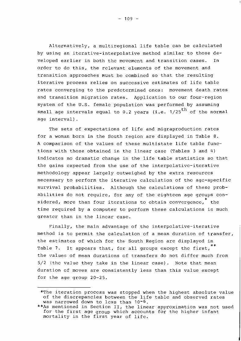
Alternatively, a multiregional life table can be calculated
by using an iterative-interpolative method similar to those de-
veloped earlier in both the movement and transition cases. In
order to do this, the relevant elements of the movement and
transition approaches must be combined so that the resulting
iterative process relies on successive estimates of life table
rates converging to the predetermined ones: movement death rates
and transition migration rates. Application to our four-region
system of the U.S. female population was performed by assuming
small age intervals equal to 0.2 years (i.e. 1 / 2 5 ~ ~ of the normal
age interval) . The sets of expectations of life and migraproduction rates
for a woman born in the South region are displayed in Table 8.
A comparison of the values of these multistate life table func-
tions with those obtained in the linear case (Tables 3 and 4)
indicates no dramatic change in the life table statistics so that
the gains expected from the use of the interpolative-iterative
methodology appear largely outweighed by the extra resources
necessary to perform the iterative calculation of the age-specific
survival probabilities. Although the calculations of these prob-
abilities do not require, for any of the eighteen age groups con- * sidered, more than four iterations to obtain convergence, the
time required by a computer to perform these calculations is much
greater than in the linear case.
Finally, the main advantage of the interpolative-iterative
method is to pe'rmit the calculation of a mean duration of transfer,
the estimates of which for the South Region are displayed in * * Table 7. It appears that, for all groups except the first,
the values of mean durations of transfers do not differ much from
5/2 (the value they take in the linear case). Note that mean
duration of moves are consistently less than this value except
for the age group 20-25.
*The iteration process was stopped when the highest absolute value of the discrepancies between the life table and observed rates was narrowed down to less than 10-6.
**As mentioned in Section 11, the linear approximation was not used for the first age group which accounts for the higher infant mortality in the first year of life.
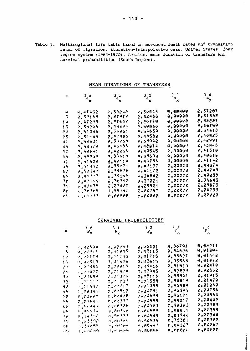
TaBle 7. Multiregional life table based on movement death rates and transition rates of migration, iterative-interpolative case, United States, four region system (1965-1970), females, mean duration of transfers and survival probabilities (South Region) .
MEAN DURATIONS OF TRANSFERS
SURVIVAL PROBABILITIES
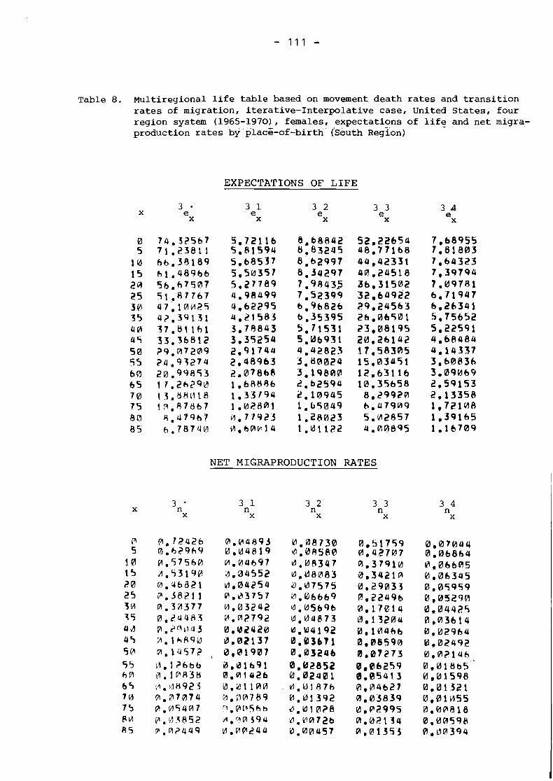
Table 8. ~ultiregional life table based on movement death rates and transition rates of migration, iterative-Interpolative case, United States, four region system (1965-19701, females, expectations of life and net migra- production rates by"plac6-of-birth- (south ~ e ~ i o n )
EXPECTATIONS OF LIFE
NET MIGRAPRODUCTION RATES
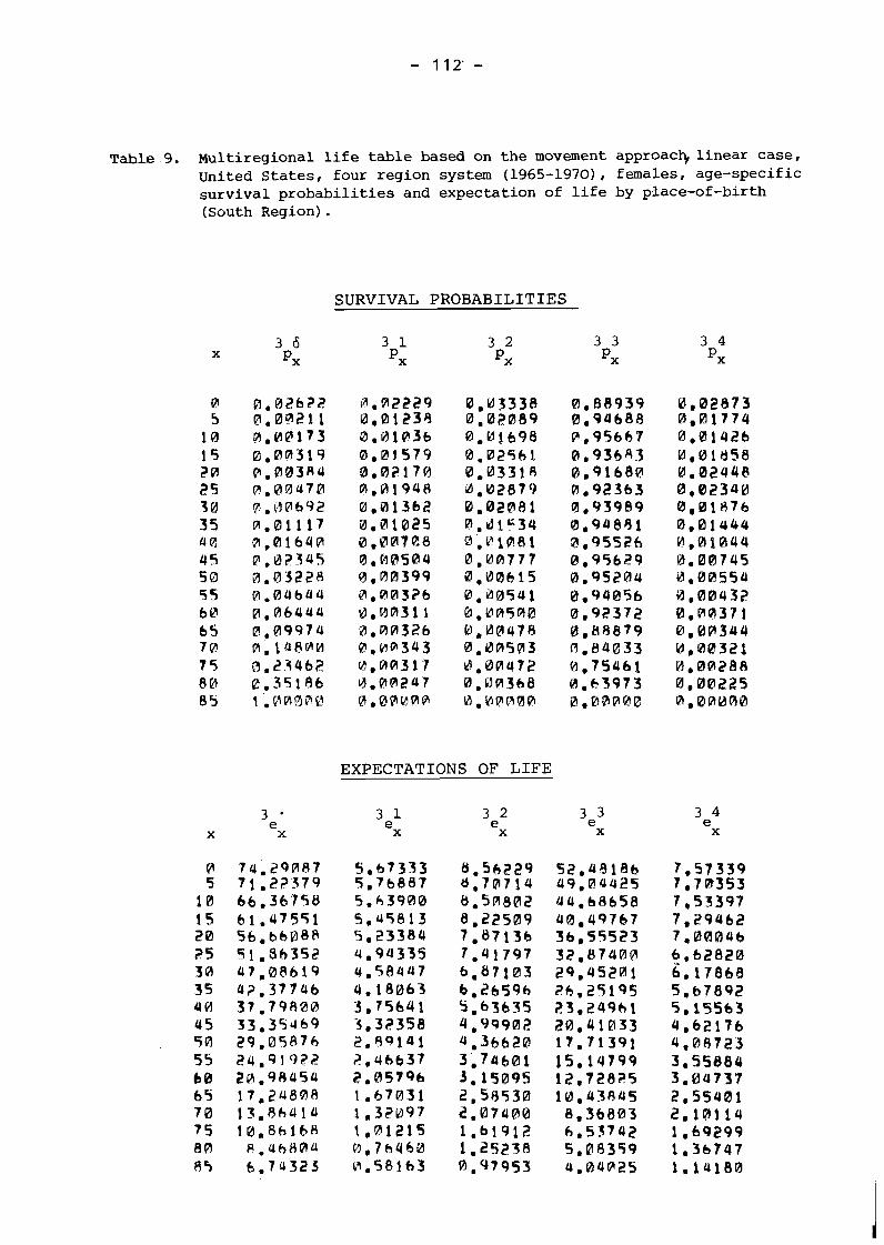
T a b l e 9. Multiregional life table based on the movement approach linear case, United States, four region system (1965-1970), females, age-specific survival probabilities and expectation of life by place-of-birth (South Region) .
SURVIVAL PROBABILITIES
p1.02622 P.Orn211 n.BPIlT3 0.D61319 pl.00384 n.0947PI r ,116692 m.01117 QI,PJ164@ Ql.dP345 8.03228 PI.BUbU4 8 . @ 6 4 4 4 @,PI9974 or , l U t 3 f l M 0 .27462 0 .35186 1 .C?VIDP\G?
EXPECTATIONS OF LIFE
Let us recall that these mean durations of transfers are 0
derived from the matrix a defined in Section 11. However, al- -X -1 though the matrix was found to be equal to I - T(1 - , - -
this last expression cannot be used to estimate 2 because a X
computer does not provide a precise estimation of the difference - 1 m between the matrices I and T(I - ex) ex -x - - . Therefore, the
0 matrix a was obtained from (49) rewritten in matrix form as: X
Numerical Assessment of the Discrepancy Between Movement, Transition, and Mixed Approaches
In order to assess numerically the discrepancy between the
alternative approaches to multiregional life table construction,
we have applied the formulas (linear case) of both the movement
and transition approaches using the age-specific rates previously
used as input data. TaSle 9 shows the survival probabilities and
expectations of life (by place-of-birth) of U.S. females in the
South region. This was obtained by constructing the multiregional
life table of the four region system of the female population
from the movement appro~ch with transition migration rates sub-
stituted for movement migration rates.
AS expected, the probabilities of dying obtained with such
a method are almost identical to those acquired earlier using
the correct mixed method. In contrast to this, the outmigration
probabilities appear to be much smaller than when correctly es-
timated, the discrepancy becoming larger in the older age groups
(compare the bottom parts of Tables 3 and 9). Thus, the use of
the movement approach when only transition rates are available,
has little consequence on the total expectations of life but may
modify the estimates of their regional shares. For example, a
woman born in the South has a life expectancy of 74.29 years
(versus 74.31) which is allocated among the regions as follows:
North East 5.67 years (versus 5.731, North Central 8.56 years
(versus 8.70), South 52.48 (versus 52.15) and West 7.57 years
(versus 7.70) .
On the other hand, constructing the multiregional life table
of the same population system from the transition approach with
movement mortality rates substituted for the transition mortality
rates leads to survival probabilities and expectation of life
(top parts of Tables 10 and 11) which only differ slightly from * their correct values (see Tables 1 and 2).
TO summarize, the type of mortalitv and migration data commonly available calls for a third approach, the mixed approach, to the
construction of a multiregional life table. Based on movement
mortality rates and transition migration rates, it is in fact,
a slightly modified variant of the transition approach in which
movement mortality rates are used as inputs rather than transition
mortality rates. It turns out that, since the discrepancy between
movement and transition mortality rates is small, the numerical
values of the multistate life table function obtained with the
mixed appraoch do not significantly differ from those obtained
with the transition approach. In contrast to this, the use of
the movement approach rather than the use of the mixed approach
would yield more inaccurate results.
Calculation of a Multiregional Life Table (Option 2)
So far, the calculation of multiregional life tables has
been performed by simply setting life table age-specific rates
equal to their observed counterparts. Rogers (1975) has devel-
oped an alternative, generalizing the census survival method
*Note that the transition approach, as developed in Section 111, does not rule out, as in Rogers' transition approach, the occur- rence of a migration followed by a death within the same unit interval. Tables 10 and 1 1 - the bottom parts of which show what the age-specific survival probabilities and expectations of llfe would be using Rogers' transition approach - indicate the necessity of using the revised approach developed here rather than Rogers' approach. For instance, ruling out the possibility for an individual to die before the end of the time period in which he has moved from one region to another, contributes to increasing the expectations of life by a large amount: in the case of the South region, life expectancy at birth then increases from 74.29 to 74.52 years.
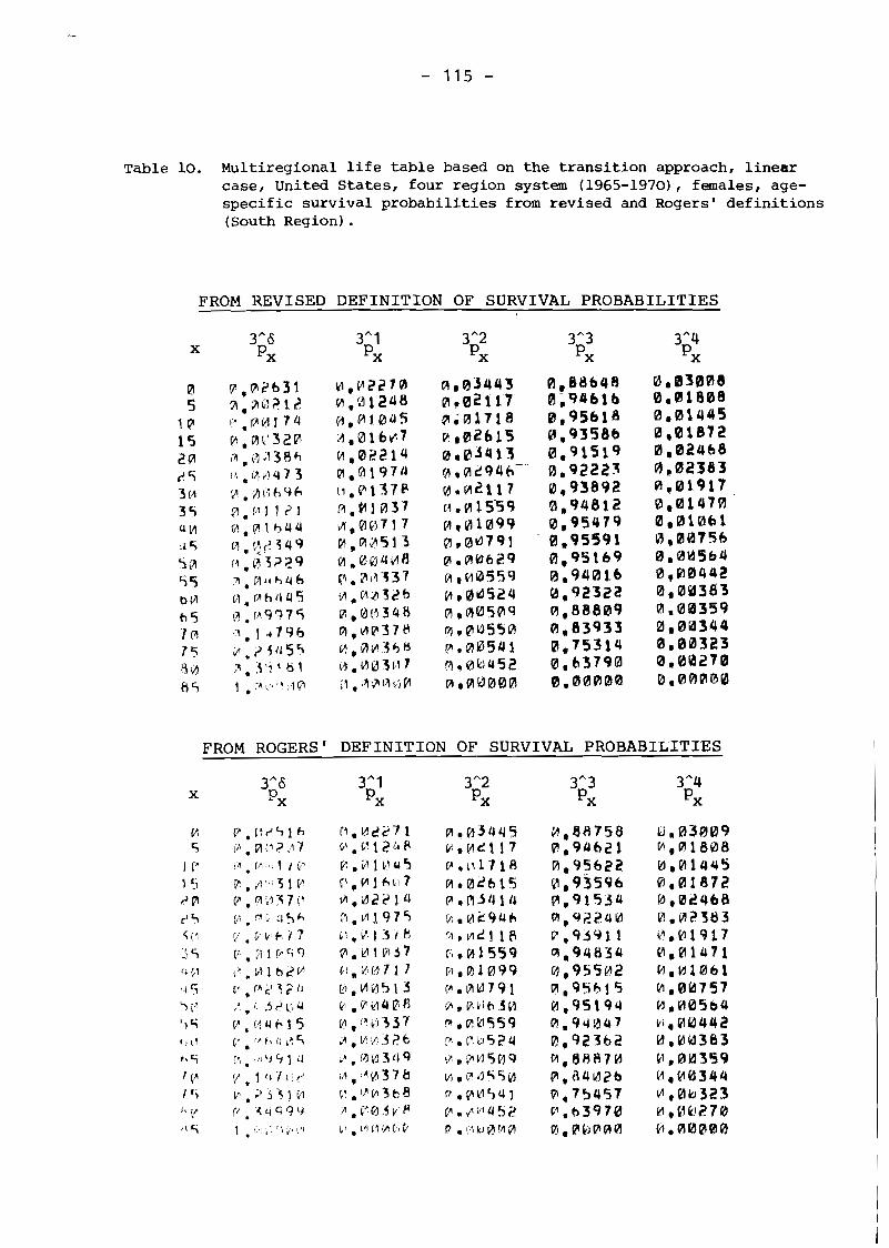
Table lo. Multiregional life table based on the transition approach, linear case, United States, four region system (1965-1970), females, age- specific survival probabilities from revised and Rogers' definitions (South Region).
FROM REVISED DEFINITION OF SURVIVAL PROBABILITIES
FROM ROGERS' DEFINITION OF SURVIVAL PROBABILITIES
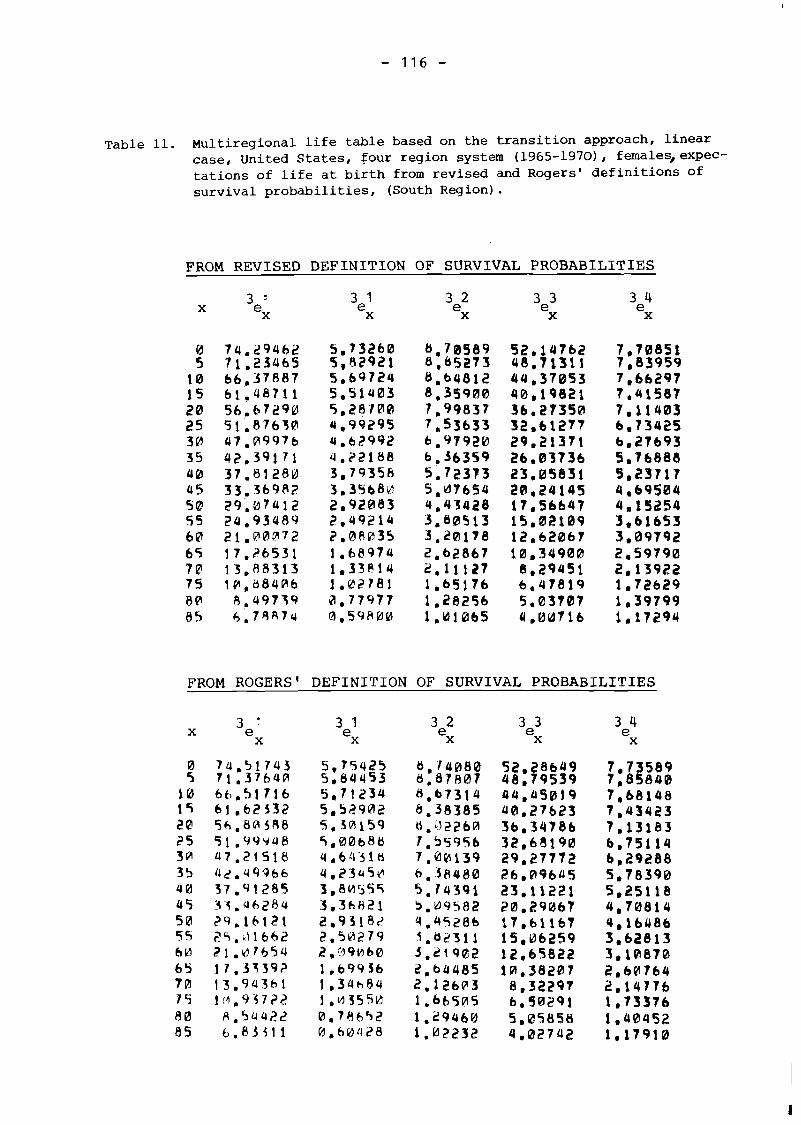
Table 11. Multiregional life table based on the transition approach, linear case, United States, four region system (1965-1970), females,expec- tations of life at birth from revised and Rogers' definitions of survival probabilities, (South Region) .
FROM REVISED DEFINITION OF SURVIVAL PROBABILITIES
FROM ROGERS' DEFINITION OF SURVIVAL PROBABILITIES
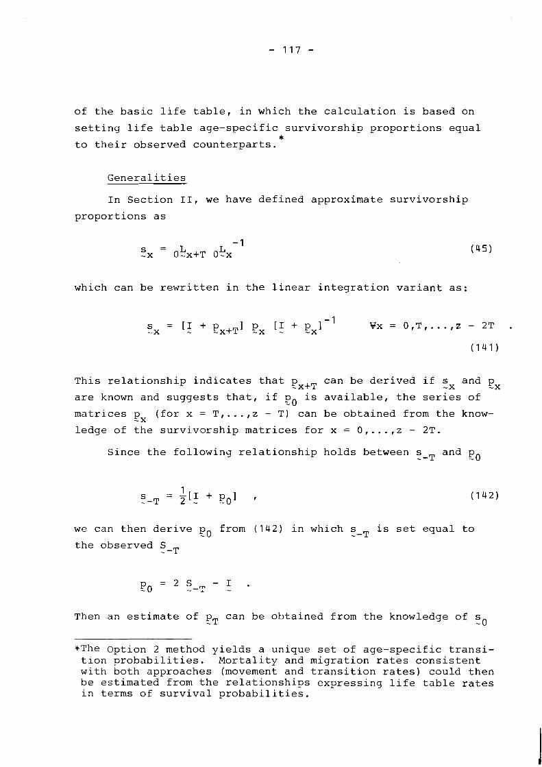
of the basic life table, in which the calculation is based on
setting life table age-specific survivorship proportions equal * to their observed counterparts.
Generalities
In Section 11, we have defined approximate survivorship
proportions as
which can be rewritten in the linear integration variant as:
This relationship indicates that p - x+T can be derived if s and p -X -X
are known and suggests that, if po is available, the series of - matrices p (for x = T I ..., z - T) can be obtained from the know- - X ledge of the survivorship matrices for x = 0, ..., z - 2T.
Since the followinj relationship holds between s-T and p - 0
we can then derive p from (142) in which s-T is set equal to - 0 the observed S-T
Then an estimate of pT can be obtained from the knowledge of s - - 0
*The Option 2 method yields a unique set of age-specific transi- tion probabilities. Mortality and migration rates consistent with both approaches (movement and transition rates) could then be estimated from the relationships expressing life table rates in terms of survival probabilities.
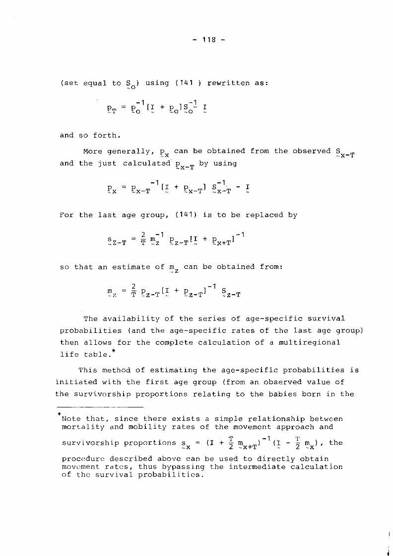
(set equal to S ) using (141 ) rewritten as: -0
and so forth.
More generally, px can be obtained from the observed S -x-T and the just calculatad by using
For the last age group, (141) is to be replaced by
so that an estimate of mZ can be obtained from: -
The availability of the series of age-specific survival
probabilities (and the age-specific rates of the last age group)
then allows for the complete calculation of a multiregional *
life table.
This method of estimating the age-specific probabilities is
initiated with the first age group (from an observed value of
the survivorship proportions relating to the babies born in the
* Note that, since there exists a simple relationship between mortality and mobility rates of the movement approach and
survivorship proportions s = -x the
procedure described above can be used to directly obtain movement rates, thus bypassing the intermediate calculation of the survival probabilities.
period considered) while Rogers' (1975) calculations proceed from
the last age group (from a value of MZ that could not be observed - and which had to be assumed).
The life table construction method just described can be
used when the information available consists of either lifetime
migration data for two consecutive censuses, or current migration
and mortality data.
Calculation from Lifetime Migration Data
Suppose that the information available consists of lifetime
migration data for two consecutive censuses, taken in years t
and t + T.
Typically, the figures available for both census years des-
cribe the regional allocation of survivors by T-year age groups
according to their place of birth. This permits the construction
of age-specif ic KY whose (i, j ) th element denotes the number of -X
persons born in region j and aged x to x + T in region i at the
time of the census (y = t and r + T) . Rogers and Von Rabenau (1971) have shown that the availabil-
ity of such data allows for a simple measurement of the observed
matrix of survivorship proportions:
In a similar way, the matrix of survivorship proportions
relating to those born during the observation period can be mea-
sured from:
in which B is a diagonal matrix whose typical element is the num-
ber of births that occurred in region i between years t and t + T.
?'hus1 lifetime migration data from two consecutive sources
permits the measurement of the series of matrices of observed
survivorship proportions allowing for the utilization of the
Option 2 method.
Calculation from Current Mortality Rates and Migration Proportions
In this alternative case, the information regarding both
mortality and mobility patterns is supposed to be identical to
that used in Option 1. The mortality data are again converted
into age-specific mortality rates consistent with the movement
approach but the migration data are now used to measure survivor-
ship proportions rather than migration rates. The problem is then one of estimating the mobility proportions that would prevail in
absence of mortality over the observation period and then using the
Option 2 method to obtain estimates of the migration rates.*
Typically, if z years and over represents the last age group z
considered, T + 2 matrices (for x = O,T, ..., z + T) describing the
transition flows (changes of residence) over the T-year period
preceding the census are needed. Let ADx denote the matrix of - ** age-specific transitions relating to age groups x to x + T
in which the flows of stayers (people present in the same region
at the beginning and end of the observation period) are included
in the diagonal.
Disregarding mortality, the fraction of those present in
region j between ages x and x + T among the group of people
present in region i, T years later is:
--
*Because age-specific mortality and migration are not independent, the miyration rates estimated here are slightly different from those that would be obtained if mortality was accounted for. -
*ti j AD denotes the number of people aged x - T to x in region i
X
at t.he beginning of the period and present in region j, T years later.
while the corresponding fraction of those born between t and
t + T in region i and present in region j at time t + T is:
In the case x = z - T I the numerator of the fraction of persons
surviving contains two terms in order to be consistent with the
treatment of the last age group in Section I1
Having measured the observed mobility proportions, we then derive
the movement rates of migration compatible with these observed
mobility proportions.
Since:
we obtain an estimate of the migration rates for the first age
group from
~n m j i in which S = ( S-T) is substituted from sT. Then the migration - -$r rates for the second age group can be obtained from (67), rewritten I
m in which S and the estimate of M just derived are substituted
, -0 - 0 for s and m and so forth. - 0 - 0
To the matrices of these migration rates are then added the
corresponding diagonal matrices of mortality rates which yields
the matrices of rates M needed to perform the calculation of a -X
multiregional life table according to the Option 1 method.
Numerical A ~ ~ l i c a t i o n
A numerical application of this method was performed from
current mortality rates and mobility proportions for the four
region system of the U.S. female population, previously considered
(the period of observation was again 1965-1970). Unfortunately,
the results turned out to be different from our expectations, since
we obtained negative outmigration rates and, consequently, neg-
ative survival probabilities for some age groups. Nevertheless,
we calculated the number of person-years lived in each age group
and found acceptable results except in the case of the last two
age groups where we obtained negative migration rates. We then
calculated the expectations of life and approximate survivorship
proportions shown in Table 12.
The question is then why the Option 2 method, unlike the
normal construction method starting from observed rates, produces
such unfortunate results. The answer is two-fold. First, the
time process of the two methods is exactly reversed. On the one
hand, the Option 1 method, based on mortality and migration * figures observed in a given point in time, calculates multistate
functions from the assumption that these mortality and migration
rates, and thus the resulting survival probabilities, remain con-
stant over time. Indeed, the survivorship proportions to which
this method lead are different from those which would be ob-
served over the data collection period. On the other hand, Option
*Although the migration data can be collected on a five-year period, the resulting migration rates are no more than averages charac- terizing the middle year of the data collection period.
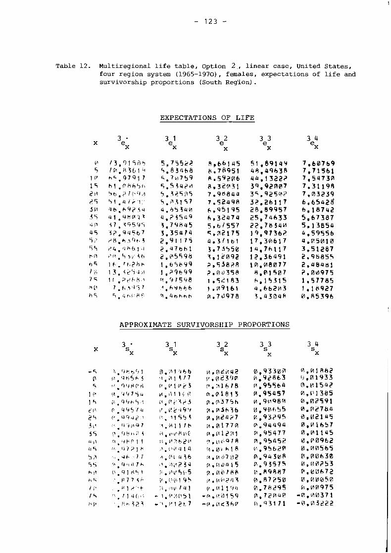
Table 12. Multiregional life table, Option 2 , linear case, United States, four region system (1965-1970), females, expectations of life and survivorship proportions (South Reg'ion).
EXPECTATIONS OF LIFE
APPROXIMATE SURVIVORSHIP PROPORTIONS
2 starts from the observation of survivorship proportions and
attenpts to determine the constant (mortality and) migration rates
or survival probabilities that would lead to such proportions.
Unfortunately, the survivorship proportions are observed for a
time period, say five years as in the above numerical illustration,
during which the age-specific migration rates are not necessarily
constant and may fluctuate greatly. Second, the nature of the
Option 2 method does not permit us to estimate mortality/mobility
rates and survival probabilities separately for each group. Since
equation (141) relates statistics of two consecutive age groups,
estimation errors made on a given age group are passed on the the
next.
In brief, since migration is a more volatile phenomenon than
mortality, (i.e., age-specific outmigration rates, unlike age-
specific mortality rates, may present large fluctuations over a
short period of time), the Option 2 method does not appear to
be as useful a method for constructing a multiregional life table
as for constructing a single-region life table.
Evaluation of the Alternative Vari.ants in ~ultiregional ~ i f e Table Construction
As just seen, the choice of the Option 2 method as a way of
constructing a multiregional life table must be avoided whenever
possible: a multiregional life table is best constructed when
using the Option 1 method based on the equalization of life table
rates with their observed counterparts.
Moreover, because of the type of mortality and mobility data
available, the mixed approach (a combination of the movement and
transition approaches) must preferably be chosen among the vari-
ations of the Option 1 method. However, the use of the trans-
ition approach yields acceptable results in view of the slight
discrepancy existing between corresponding movement and transition
death rates. That statement would not be true if the movement
approach was used instead. In other words, in contrast to the * analysis of life status (Schoen and Nelson, 1974; Schoen, 1975)
the study of interregional migration generally requires the choice
of the mixed approach which is closely related to the transition
approach.
It is clear that the most feasible integration methods to
derive { L 1 are the linear and cubic integration methods. However, X
in contrast to the linear method that can be easily used whatever
the approach chosen (movement, transition, mixed), the cubic method
can only be used in the case of the movement approach. Since
movement migration data are sometimes available, we have used this
integration method to calculate a multiregional life table of the
four region system for the U.S. female population in which the
values of the observed transition rates were substituted for those
of the movement rates. The age-specific survival probabilities
thus obtained (Table 13) were then directly comparable with the
ones similarly obtained when using a linear integration method
( Takle 9).
The result is that: a) the cubic integration method does
not yield radically different estimates, b) the discrepancy be-
tween the linear and cubic estimates mostly affects the retention I
probabilities and the probabilities of dying, and c) this dis- I
I crepancy tends to be higher for older ages (see age qroup 75 to * * 80). The mean durations of transfers implied by the choice of
the cubic integration method appear in the bottom part of Table 13.
The discrepancies between the linear and cublc integration
methods on the one hand, and the linear and the interpolative-
iterative methods on the dther hand point in opposite directions.
Whereas the interpolative-iterative method yields higher retention
probabilities and smaller probabilities of dying than the linear
integration method (as suggested by the comparison of the survival
*The type of data available for the problem studied by Schoen makes the use of the movement approach preferable.
**The estimates of the survival probabilities for age groups 5 to 10 and 80 to 85 were identical in both Tables 9 and 13 since the linear integration method was substituted for the cubic integra- tion method.
probabilities in Tables 3 and 7), the cubic integration method
yields smaller retention probabilities and higher probabilities
of dying. Also, the interpolative-iterative method yields 6 (see Table 7) ax coefficients slightly higher than 2.5 (except
for the first age group), while the cubic integration method
leads to a: coefficients much higher than 2.5 (see able 13).
If the interpolative-iterative method is assumed to be more
accurate than any other method, it then appears that the linear
integration method yields estimates of the multistate life table
functions which are better than those of the cubic integration
method. Then, even if its use is made possible by the type of
data available, the cubic integration method will not be prefered
to the linear integration method. Moreover, since the interpolative-
iterative method yields estimates of the multistate life table
functions only slightly different from those obtained in the linear
case, the linear integration method would generally be prefered
because of the larger computer time required for the interpolative-
iterative method.
Finally, the mixed approach of the Option 1 method based on
a linear integration over {l } for deriving { L ~ } appears as the Y
best variant in calculating a multiregional life table.*
Migration Rates and the Calculation of a ~ultiregional Life Table
Clearly, the accuracy of the columns of a multiregional life
table calculated by the Option 1 method depends on the precision
of observed mortality and mobility rates' measurement.
Impact of Alternative Measures of ran sit ion Migration Rates
Whereas the measurement of movement rates as proposed by
(134) and (135) does not raise any particular problem (straight-
forward extension of the single region case), the measurement of
transition rates suggested in (136) and (137) raises some difficul-
ties because the numerators and denon~inators of these definitions
*The present conclusion is indeed limited to the case of a demo- graphic system for which available data are movement mobility data and transition migration data. However, it can be extended to the case of any demographic system, as we will see later.
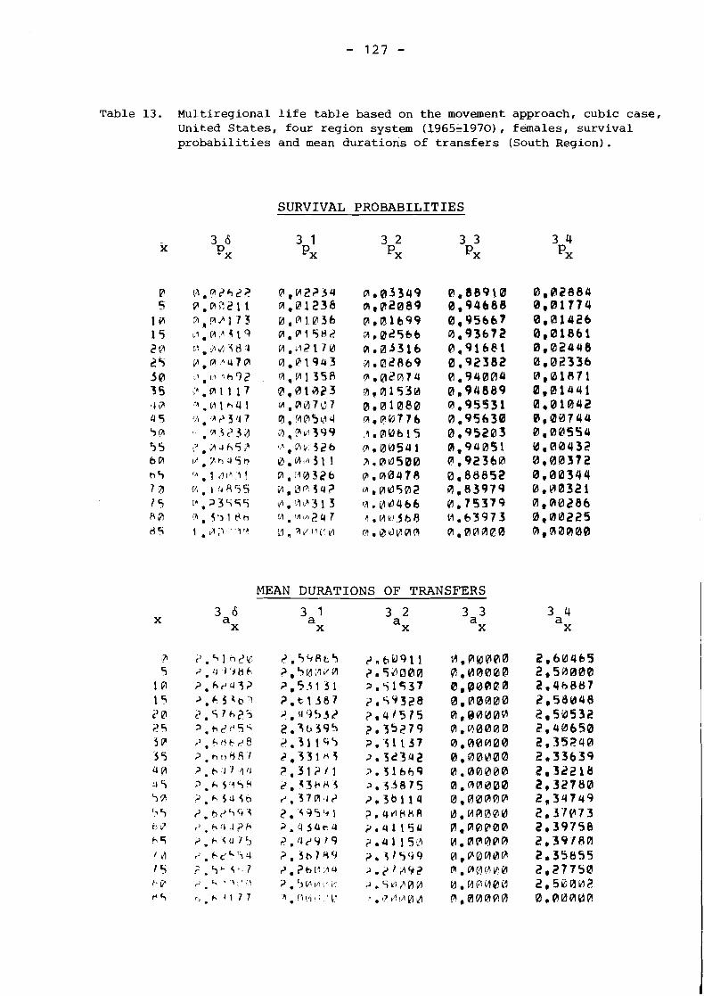
Table 13. Multiregional l i f e table based on the movement approach, cubic case, United States, four region system (1965&1970), females, survival probabi l i t ies and mean durations of t ransfers (South Region).
SURVIVAL PROBABILITIES
MEAN DURATIONS OF TRANSFERS
must be approximated. As a matter of fact, Rogers (1975a) proposes
approximations of these quantities different from those put down
earlier in this paper. He simply measures the rate of migration
from region i to region j for age group x, x + T as the ratio of
the number of changes of residence (from i to j made during the
observation period by those aged x to x + T at the end of the
interval) to the average population in region i, i.e.,
iA j Clearly, this contrastswith our measurement of m defined as
X
a relationship obtained by combining (137) through (139).
The alternative measures of migration rates out of the South
Region in our four region system of the U.S. calculated from (143)
and (144) appear in Table 14 which shows that transition migration
rates as measured by (143) are generally higher than when measured
by (144).
Since the denominators of in both (1 43) and (144) take X
similar values, the discrepancy between our measurement method
and that of Rogers originates for the larqer part from the dif-
ferent values taken by the numerators of (143) and (144). Indeed,
the numerator of (143) concerns migrants who were aged x to x + T
at the end of the observation period, while the numerator of (144)
represents an approximation of the number of migrations from region
i to region j relating to the people aged x to x + T in the middle
year of the observation period. Clearly, our measurement method
(144) is more legitimate than that of Rogers (143) which does not
properly estimate the age disaggregation of migration flows over
the observation period.
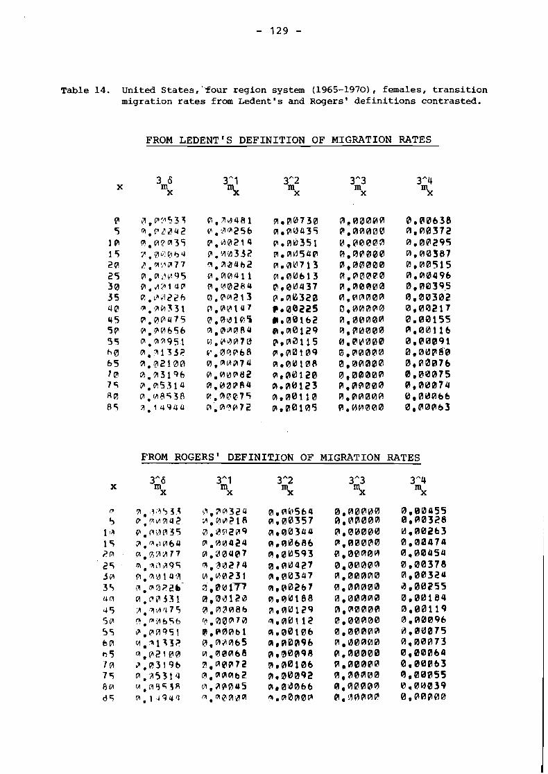
Table 14. United States,"four region system (1965-1970), females, transition migration rates from Ledent's and Rogers' definitions contrasted.
FROM LEDENT'S DEFINITION OF MIGRATION RATES
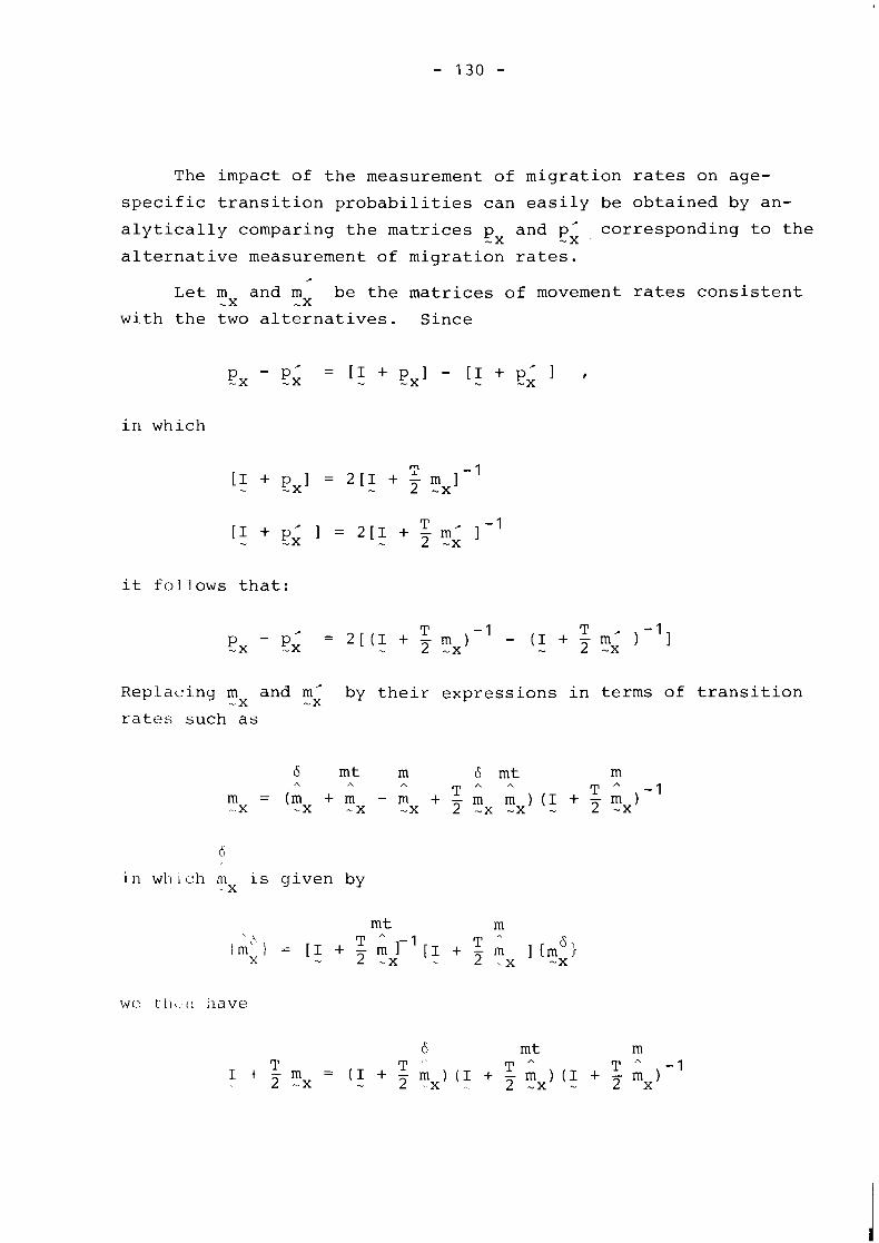
The impact of the measurement of migration rates on age-
specific transition probabilities can easily be obtained by an-
alytically comparing the matrices p and p' corresponding to the -x -X alternative measurement of migration rates.
' Let mx and m be the matrices of movement rates consistent - -X
with the two alternatives. Since
in which
it follows that:
Replacing m and m' by their expressions in terms of transition - X -X
rates such as
in which m is given by - . X
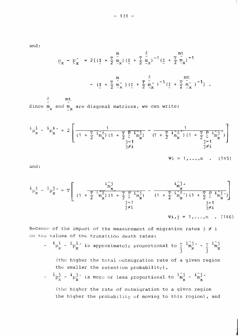
and :
6 mt A A
Since m and m are diagonal matrices, we can write: - x , x
and :
Becausv of the impact of the measurement of migration rates j # i
o11 t l ~ ~ values of the trdnsitio~l death rates:
i i A
- - i i. imj, iA j x is approximately proportional to 1
X
(the higher the total outmigration rate of a given region
the smaller the retention probability),
.- i j - i j, iAj iAj, px px X X
is more or less proportional to m - m
(the higher the rate of outmigration to a given region
the higher the probability of moving to this region), and
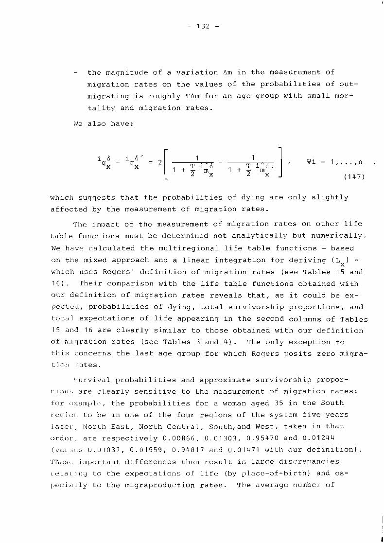
- the magnitude of a variation Am in the measurement of
migration rates on the values of the probabilities of out-
migrating is roughly TAm for an age group with small mor-
tality and migration rates.
We also have:
which suggests that the probabilities of dying are only slightly
affected by the measurement of migration rates.
The impact of the measurement of migration rates on other life
table functions must be determined not analytically but numerically.
We have calculated the multiregional life table functions - based
on the mixed approach and a linear integration for deriving {L - X
which uses Rogers' definition of migration rates (see Tables 15 and
16). Their comparison with the life table functions obtained with
our definition of migration rates reveals that, as it could be ex-
pected, probabilities of dying, total survivorship proportions, and
totdl expectations of life appearing in the second columns of Tables
15 and 15 are clearly similar to those obtained with our definition
of n.icjration rates (see Tables 3 and 4). The only exception to
this concerns the last age group for which Rogers posits zero migra-
!;11i-viva1 probabilities and approximate survivorship propor-
111,1~-, are clearly sensitive to the measurement of migration rates:
for r txc~~~pl t . , the probabilities for a woman aged 35 in the South
reqic~~, to he in one of the four reqions of the system five years
later , Nor t:h East, North Central, South, and West, taken in that
order, are respectively 0.00866, 0 01303, 0.95470 and 0.01244
(ve~c,~ls 0.01037, 0.01559, 0.94817 and 0.01471 with our definition). I I I t i ~ : ; ~ 1111t~orta11t differences then result in large discrepancies
el at l l i y to the expectations of life (by ~jldze-of-birth) and es-
I , c c : ~ d Lly to the migraproduction rates. The average numbei of
moves out of the four U.S. census reuions made by a woman born
in the South region decreases from 0.72 (with our definition) to
0.59 (with Rogers ' definition) . In brief, the columns of a multiregional life table are very
sensitive to the proper measurement of migration rates as illus-
trated Sy the above comparison of two multiregional life tables
constructed with alternative definitions of the migration rates.
Moreover, it was shown that the discrepancy resulting from these
two alternative definitions was much higher than the discrepancies
implied by the theoretical points of choice, i -e- t the choice between
the transition and movement approaches or the choice between the
linear method of integration and the interpolative-iterative method.
Influence of the Length of the Observation Period
Again, since the measurement of observed movsment rates is
a straightforward extension of the measurement of observed rates
in the sinule-region case, the length of the time interval over
which actual movement rates are observed does not raise any par-
ticular difficulty. However, as put forward at the beginning of
this section, the correct measurement of transition migration
rates for use in an increment--decrement life table implicitly
requires that the length of the typical age group be equal to the
duration of the period over which migration is recorded. Thus,
the numerical applications concerning our U.S. four-region system
were carried out from migration data relating to five-year age
groups observed on a five-year period (1965-70).
It is clear that if the migration data had been available
for a one-year period only, the resulting migration rates would
have led to an overestimation of the probabilities of moving
from one region to another. Intuitively, this problem stems from
the well known fact that annual migration rates are higher than
l/nth time n-year migration rates, owing to the peculiarities
caused by multiple moves and especially return migration. (See
Table 17 comparing typical one-year and five-year migration rates
for British regions.)
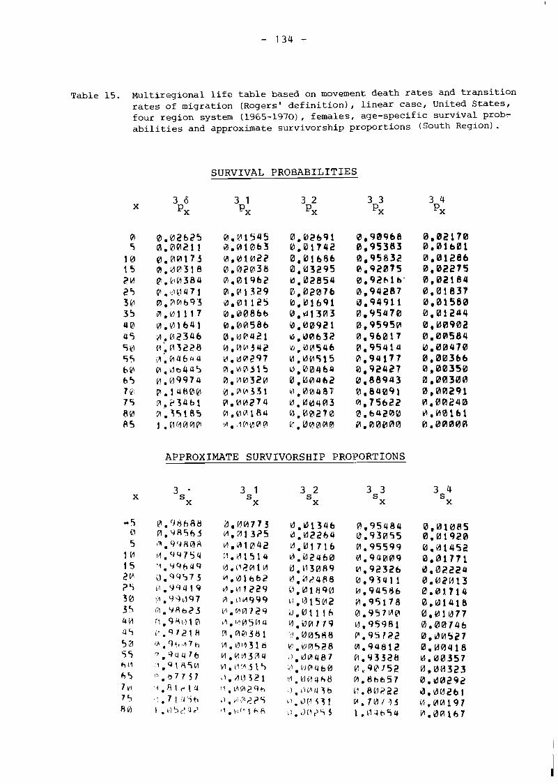
Table 15. Multiregional l i f e t ab le based on movement death ra tes and t r ans i t i on r a t e s of migration (Rogers' de f i n i t i on ) , l i near case, United S ta tes , four region system (1965-1970) , females, age-specif ic surv ival prob- a b i l i t i e s and approximate survivorship proportions (South Region).
SURVIVAL PROBABILITIES
APPROXIMATE SURVIVORSHIP PROPORTIONS
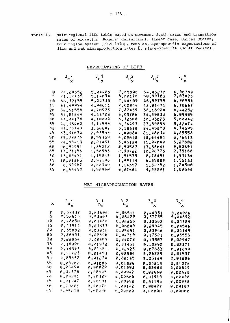
Table 16. Multiregional life table based on movement death rates and transition rates of migration (Rogers' definition), linear case, United States, four region system. (1965-1970) , females, age-specif ic expectations .of life and net migraproduction rages by place-~f-birth ( ~ o h t h Region) .
EXPECTATIONS OF LIFE
NET MIGRAPRODUCTION RATES
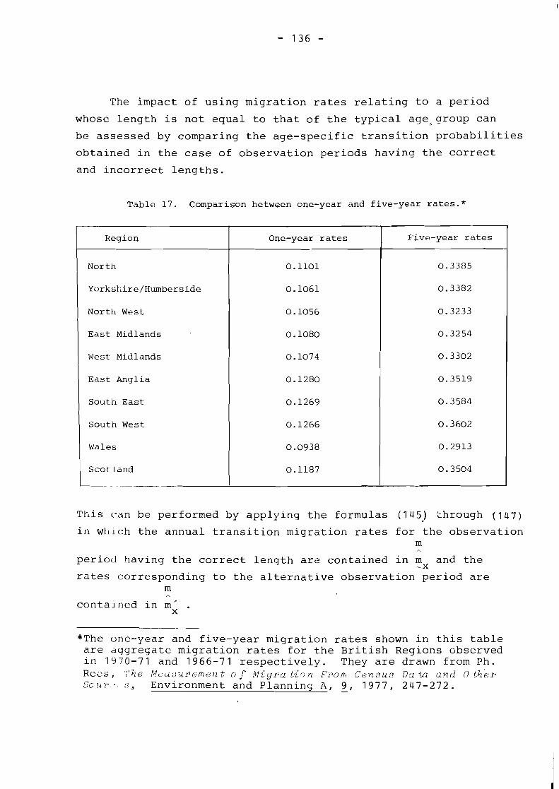
The impact of using migration rates relating to a period
whose length is not equal to that of the typical acjepgroup can
be assessed by comparing the age-specific transition probabilities
obtained in the case of observation periods having the correct
and incor,rect lengths.
Table 17. Comparison between one-year and five-year rates.*
This can be performed by applying the formulas (145) through (147)
Region
North
Yorkshire/~umberside
North West
East Midlands
West Midlands
East Anglia
South East
South West
Wales
Scot land
-
in which the annual transition migration rates for the observation m
period having the correct length are contained in mx and the -
One-year rates 1 B'ive-year rates
rates corresponding to the alternative observation period are m n
contained in m' . X
0.1101
0.1061
0.1056
0.1080
0.1074
0.1280
0.1269
0.1266
0.0938
0.1187
*The one-year and five-year migration rates shown in this table are aggregate migration rates for the ~ r i t i sh Regions observed in 1970-71 and 1966-71 respectively. They are drawn from Ph. Rees, ' f h e Mt l~csurement o f M ig ra t i i i n From C e n s u s Da ta and o t h e r S O ~ ~ Y J ' - ~ S, Environment and Planning A, 9 , 1977, 247-272. -
1
0.3385
0.3382
0.3233
0.3254
0.3302
0.3519
0.3584
0.3602
0.2913
0.3504
Since m is generally much less than m' -.65 n' in the -X -x (mx - -X
case of the British regions shown in Table 17), it follows that
the use of annual migration data instead of five-year migration
data i n a model in which population is broken down into five-year
age groups leads to inaccurate estimates of the multiregional
life table functions. This is illustrated by the comparison of
Tables 18 and 19 displaying four multiregional life table functions
(survival probabilities, approximate survivorship proportions,
expectations of life and migraproduction rates) obtained by mul-
tiplying all transition rates of our U.S. four-region example
by 1/0.65 - with those of Tables 3 and 4.
For example, the life expectancy of a woman born in the South
slightly increased form 74.31 to 74.39 years while the times of
this life expectancy spent in other regions increase dramatically:
5.73 to 7.50 (North East), 8.71 to 11.2 (North Central) and 7.70
to 10.09 (West). The higher mobility is also reflected by the
total migraproduction rate for a woman born in the South which
jumps from .72 to 1.13.
Clearly, the difficulties relating to the measurement of
migration rates (more specifically number of moves or transitions,
length of the period of observation) have an impact on the calcula-
tion of multiregional life tables that is much larger than those
created by methodological aspects. In the future, improved methods
for calculating multiregional life tables should not focus so
much on extending theoretical grounds (developed in this paper)
but rather on proposing better methods of measuring migration
rates from data commonly available.
Comparison of the Actual and Modeled Migration Processes
One of the strengths of the single-state life table is that
its underlying mortality process replicates the actual mortality * process. The reason for this is that the propensity to die at
*The discrepancy between actual and modeled mortality processes results from the more or less regular age camposition of the ob- served population (owing to variations in the fertility pattern and, at a lesser degree, in the mortality pattern over time).
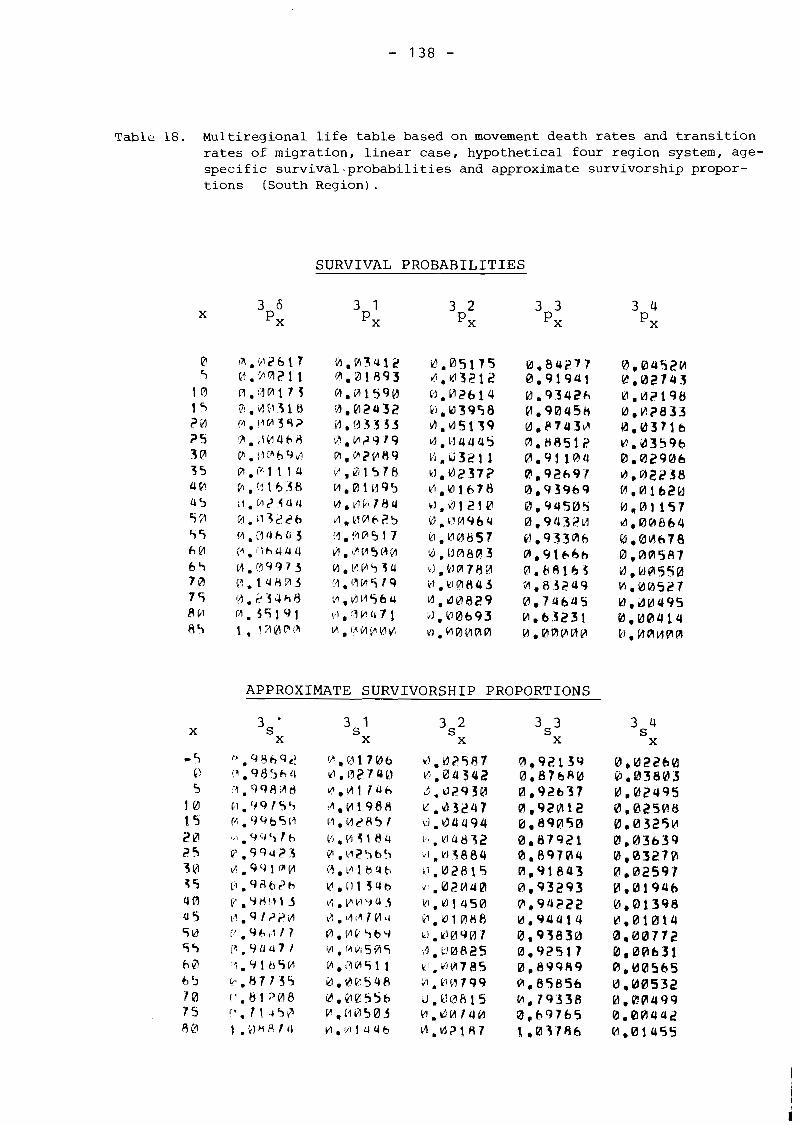
Table 18. Multiregional life table based on movement death rates and transition rates of migration, linear case, hypothetical four region system, age- specific survival.probabilities and approximate survivorship propor- tions (South Region).
SURVIVAL PROBABILITIES
APPROXIMATE SURVIVORSHIP PROPORTIONS
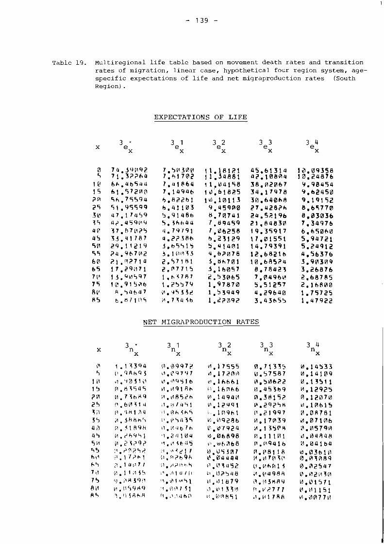
Table 19. Multiregional l i f e table based on movement death ra tes and t rans i t ion ra tes of migration, l inear case, hypothetical four region system, age- spec i f ic expectations of l i f e and net migraproduction ra tes (South Region) .
EXPECTATIONS OF LIFE
NET MIGRAPRODUCTION RATES
any age y in an observed population is roughly the same for all
individuals of each age cohorts as hypothesized in the life table
(this propensity to die only depends on the value of y ) .
Does the multiregional life table provide a similar duplica-
tion of the actual mobility process between regions of the system?
First, note that the single-region assumption of homogeneous age
cohorts cannot be extended to the rnultiregional case because the
propensities to migrate vary among individuals in a very sensitive
manner. Some individuals ("chronic" movers) have a tendency to
move repeatedly. In actual populations, members of a group of
individuals present at the same age in a given region have dif-
ferential propensities to move, largely dependent on their past
migratory history; the larger the number of moves made in the past,
the higher their propensity to move.
The question is one of determining how unrealistic the as-
sumptions contained in the multiregional life table are. What-
ever the focus chosen (movement or transition approach), the
multiregional life tabie (or more generally the increment-decrement
life table) is in fact concerned with transitions between predeter-
mined ages rather than with moves: in essence, it looks at net *
balances of migrations rather than at gross migration flows.
The multiregional life table thus describes a (Markovian)
transition scheme in which the consolidation of moves into transi-
tions occurs within the model (movement approach) rather than out-
side of the model (transition approach) . 'The multiregional life table must be judged on its ability
to replicate consolidated moves (transitions) rather than gross
flows (moves). Let us summarize the two main alternatives (move-
ment and transition approaches).
*The rnultiregional life table functions generally relate to age- cohorts independently of the region of presence at any earlier age and only require the knowledge of consolidated moves (an exceI)tion to this is the case of migraproduction rates).
First, the movement approach permits us to calculate all
moves accurately but not transitions because of the non-validity
of the Markovian assumption in the real world (multiplying by x
movement rates would result in an approximate multiplication by
x of transition rates).* Therefore, its use is to be avoided
when calculating a multiregional life table.
Second, the transition approach makes it possible to calcu-
late accurately observed transitions if the transition migrations
are appropriately chosen (i.e., if the length of the typical age
group is equal to the length of the observation period).
The homogeneous and Markovian assumptions underlying the
multiregional life table seriously limit the ability of the multi-
regional life table to replicate the observed migration process.
On the one hand, the movement approach may lead to the duplication
of gross moves but not to that of consolidated moves. On the other
hand, the transition approach allows for a "reduced-form" dupli-
cation of transitions or consolidated moves, which fortunately is
sufficient to calculate most multiregional life table columns.
A further consequence is that the movement migration rates
whic11 were derived earlier in this section, in agreement with the
transition migration rates, were not true movement rates, but were
those which led to the same multiregional life table as the trans-
ition migration rates.
*The use of the Markovian assumption keeps multiple moves (and especially return moves) at a low level. For example, in the case of a two-region system, the ratio of return moves to the gross outmigration flow can be obtained as
CONCLUSION
The most important feature of combined life tables that
allow entries as well as withdrawals, is the existence of more
than one stationary population in the multi-radix case. If indi-
viduals are born in at least two states of the population system
at hand, the solution of the differential equation ( 1 7 ) underly-
ing such life tables shows that all are linear combinations of
the r independent stationary populations generated by the sur-
vivors of each state-specific group of the initial cohorts. Con-
sequently, in the case of more than one radix, life table func-
tions characteristic of age groups depend on the relative weight
accorded to the r independent stationary populations, i.e. depend
on the state allocation of the initial cohort.
The consequence is that the construction of a coherent incre-
ment-decrement life table requires the additional assumption of
the independence of life table rates vis-a-vis the allocation of
the initial cohort. It is not correct to state that the defini-
tion (35) of movement rates
is equivalent to ( 6 1 )
( 1 4 9 ) implies ( 1 4 8 ) , but ( 1 4 8 ) does not imply ( 1 4 9 ) . In fact,
there is equivalence only if ( 1 4 8 ) holds not only for the whole
stationary population but also for the independent stationary
populations generated by each radix of the initial cohort:
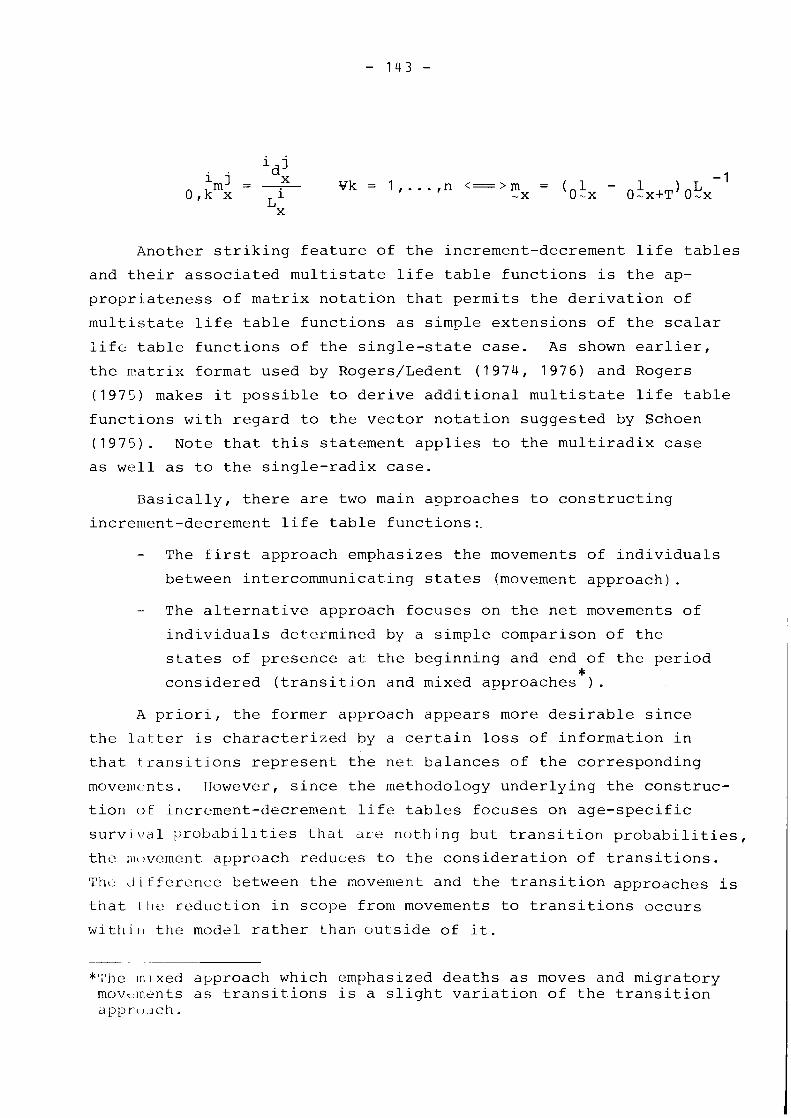
Another striking feature of the increment-decrement life tables
and their associated multistate life table functions is the ap-
propriateness of matrix notation that permits the derivation of
multistate life table functions as simple extensions of the scalar
life table functions of the single-state case. As shown earlier,
the matrix format used by Rogers/Ledent (1974, 1976) and Rogers
(1975) makes it possible to derive additional multistate life table
functions with regard to the vector notation suggested by Schoen
(1975). Note that this statement applies to the multiradix case
as well as to the single-radix case.
Basically, there are two main approaches to constructing
increment-decrement life table functions:.
- The first approach emphasizes the movements of individuals
between intercommunicating states (movement approach).
- The alternative approach focuses on the net movements of
individuals determined by a simple comparison of the
states of presence aL the beginning and end of the period * considered (transition and mixed approaches ) .
A priori, the former approach appears more desirable since
the l<ltter is characterized by a certain loss of information in
that transitions represent the net balances of the corresponding
movenients. FIowever, since the methodology underlying the construc-
tion of increment-decrement life tables focuses on age-specific
survlval probabilities that dre nothing but transition probabilities,
the nlovernent approach redu~es to the consideration of transitions.
Thc ~llfference between the movement and the transition approaches is
that Ille reduction in scope from movements to transitions occurs
wlt-hl~l the model rather than outside of it.
- --- ---
*The Inlxed approach which emphasized deaths as moves and migratory mov~ments as transitions is a slight variation of the transition d p p r u lch.
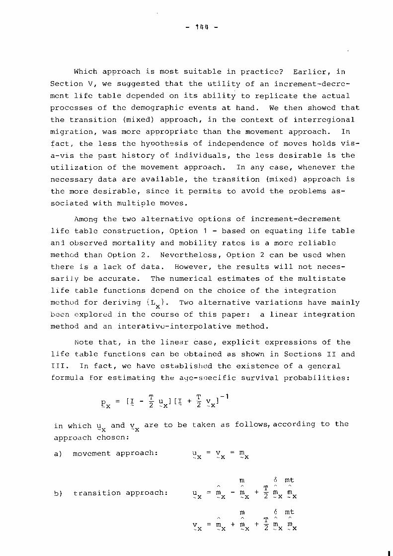
Which approach is most suitable in practice? Earlier, in
Section V, we suggested that the utility of an increment-decre-
ment life table depended on its ability to replicate the actual
processes of the demographic events at hand. We then showed that
the transition (mixed) approach, in the context of interregional
migration, was more appropriate than the movement approach. In
fact, the less the hypothesis of independence of moves holds vis-
a-vis the past history of individuals, the less desirable is the
utilization of the movement approach. In any case, whenever the
necessary data are available, the transition (mixed) approach is
the more desirable, since it permits to avoid the problems as-
sociated with multiple moves.
Among the two alternative options of increment-decrement
life table construction, Option 1 - based on equating life table
an3 observed mortality and mobility rates is a more reliable
method than Option 2. Nevertheless, Option 2 can be used when
there is a lack of data. However, the results will not neces-
sarily be accurate. The numerical estimates of the multistate
life table functions depend on the choice of the integration
method for deriving {L~} . Two alternative variations have mainly
been explored in the course of this paper: a linear integration
method and an interative-interpolative method.
Note that, in the linear case, explicit expressions of the
life table functions can be obtained as shown in Sections I1 and
111. In fact, we have established the existence of a general
formula for estimating the aye-s~~ecific survival probabilities:
in which ux and yx are to be taken as followslaccording to the
approach chosen:
a) movement approach:
m 6 mt A A
5 ) transition approach: T " "
u = m - m + - m m -X -X x 2 - x --X
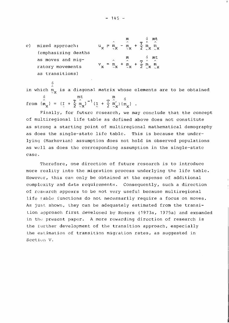
m A A
6 mt
c) mixed approach: T A A u ~m - m + - m m X -x -x 2 ,x ,x
(emphasizing deaths
A
m as moves and mig- A
6 mt r n " A
v = m + m +'m m ratory movements x -x -x 2 ,x ,x
as transitions)
6 A
in which m is a diagonal matrix whose elements are to be obtained -X
A T A -1 n A 0
from {mxl = (I + mx) (I + m' ) { .- ... 2 -x mxl .
Finally, for future research, we may conclude that the concept
of multiregional life table as defined above does not constitute
as strong a starting point of multiregional mathematical demography
as does the single-state life table. This is because the under-
lying (Markovian) assumption does not hold in observed populations
as well as does the corresponding assumption in the single-state
case.
Therefore, one direction of future research is to introduce
more reality into the migration process underlying the life table.
However, this can only be obtained at the expense of additional
complexity and data requirements. Consequently, such a direction
of research appears to be not very useful because multiregional
life table functions do not necessarily require a focus on moves.
A s just shown, they can be adequately estimated from the transi-
tion approach first developed by Roqers (1973a, 1975a) and expanded
in the present paper. A more rewarding direction of research is
the further development of the transition approach, especially
the estimation of transition migration rates, as suggested in
Sectic)~l V.
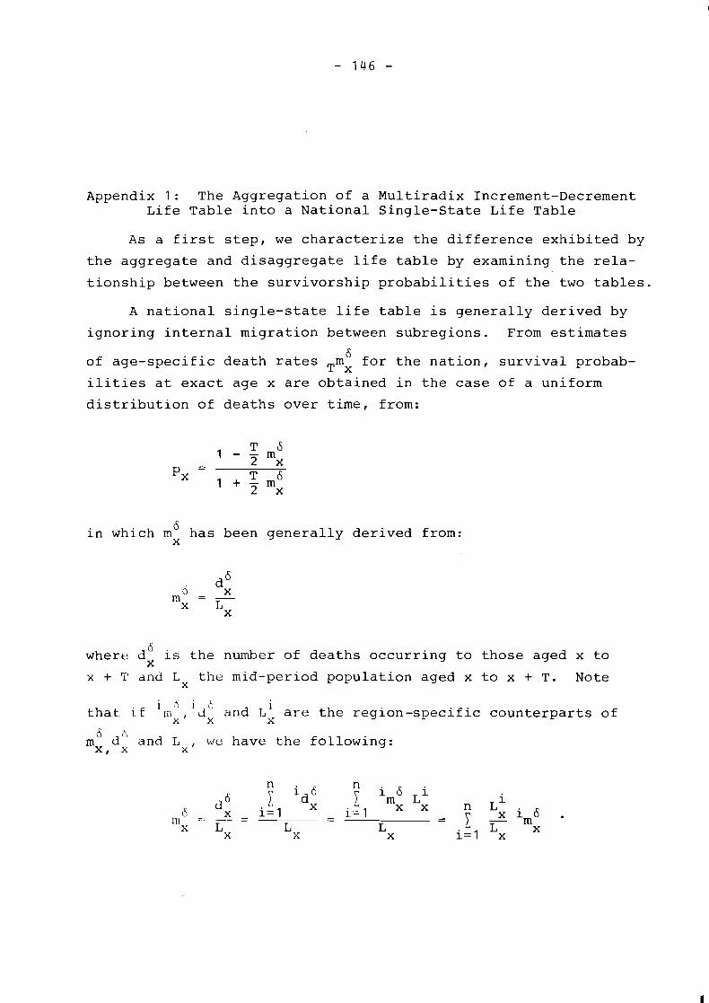
Appendix 1: The Aggregation of a Multiradix Increment-Decrement Life Table into a National Single-State Life Table
As a first step, we characterize the difference exhibited by
the aggregate and disaggregate life table by examining the rela-
tionship between the survivorship probabilities of the two tables.
A national single-state life table is generally derived by
ignoring internal migration between subregions. From estimates
of age-specific death rates Tm2 for the nation, survival probab-
ilities at exact age x are obtained in the case of a uniform
distribution of deaths over time, from:
in which m6 has been generally derived from: X
where d 6 is the number of deaths occurring to those aged x to X
x + 1' and Lx the mid-period population aged x to x + T. Note
i ? i that. i ~ f rn dx and 1; are the region-specific counterparts of
x X
m6 d: and L x , w e have the following: x,
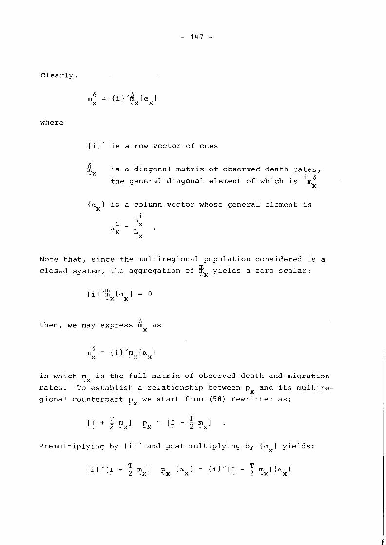
Clearly:
where
{i)' is a row vector of ones
is a diagonal matrix of observed death rates, m -x i 6 the general diagonal element of which is m X
{u is a column vector whose general element is X
Note that, since the multiregional population considered is a
closed system, the aggregation of gx - yields a zero scalar:
6 then, we may express m as
X
in which m is the full matrix of observed death and migration - X rates. To establish a relationship between px and its multire-
gional counterpart p we start from (58) rewritten as: -x
Premultiplying by ti}' and post multiplying by { a ) yields: X
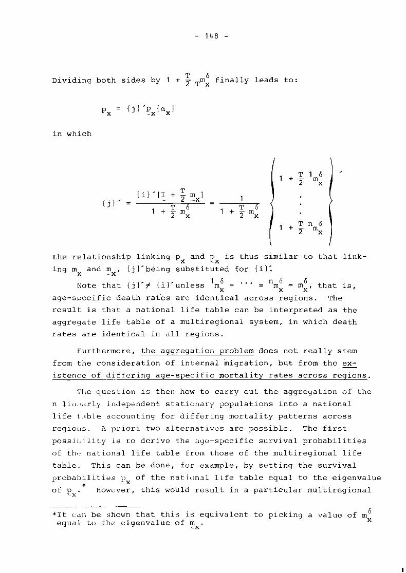
T Dividing both sides by 1 + Tm: finally leads to:
px = {jl'p {ax) ." x
in which
the relationship linking p and p is thus similar to that link- X -X
ing m and m , { j )'being substituted for t i ) : X -X
1 6 ... - n 6 Note that { j )'# {i)'unless m = - 6
x m x = m x that is, age-specific death rates are identical across regions. The
result is that a national life table can be interpreted as the
aggregate life table of a multiregional system, in which death
rates are identical in a11 regions.
Furthermore, the aggregation problem does not really stem
from the consideration of internal inigration, but from the - ex-
istence of - differing age-specific mortality rates across regions.
The question is then how to carry out the aggregation of the
n li11,darly illdependent statior1a~-y populations into a national
l.ife t.lble accounting for differing mortality patterns across
regio~ls. A priori two alternatives are possible. The first
possit.1i1it.y is to derive the age-specific survival probabilities
of tht: national life table fro1~1 those of the multiregional life
table. This can be done, for example, by setting the survival
probabilities p of the national life table equal to the eigenvalue * X of p . However, this would result in a particular multiregional
- X
-. -- -. - - - -- -- - +It cdn be shown that this is equivalent to picking a value of m 6
equal to ths eigenvalue of m-,. X - A
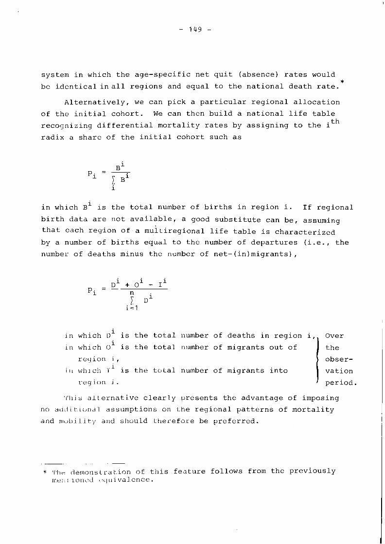
system in which the age-specific net quit (absence) rates would * be identical inall regions and equal to the national death rate.
Alternatively, we can pick a particular regional allocation
of the initial cohort. We can then build a national life table
recognizing differential mortality rates by assigning to the i th
radix a share of the initial cohort such as
in which B~ is the total number of births in region i. If regional
birth data are not available, a good substitute can be, asauming that each region of a multiregional life table is characterized
by a number of births equal to the number of departures (i.e., the
number of deaths minus the number of net-(in)migrants),
i ln which D is the total number of deaths in region i f
in whlch oi is the total number of migrants out of
reyion 1, i
1 1 1 which I is the total number of migrants into
region 1.
#it I 11~~s . alternative clearly presents the advantage of imposing
no ad~iit-.iondl assumptions on Lhe regional patterns of mortality
and n~cjbi 1 i. ty and should therefore be preferred.
- -. - -
* ' r h ~ (3emonstrat.ion of tilis feature follows from the previously r n e 1 1 I lorit?d 1.cluiva1 ence.
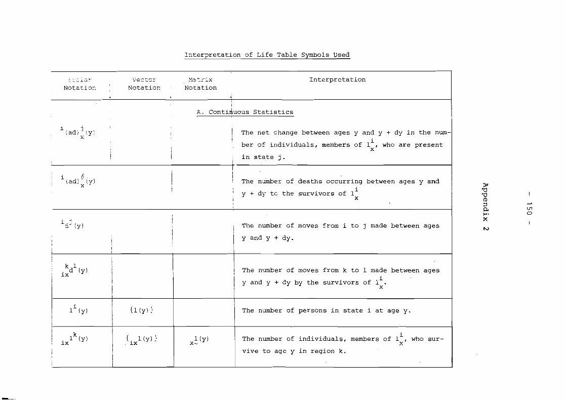
I z t e r ~ r e t a t i o n of L i fe Table Svmbols Used
- - LZZLZZ- v e c t z r Mzt r - x In terpretac ion
Nota~l3r . Notat lor Norahon 4 I
P-. ~on t l duous S t a t l s t l c s
1 ladi:!y: ' The ne t change between ages y and y + dy i n the num- I I i ! ber of ~ n d i v i d u a l s , members of 1 , who a re present X
! i i n s t a t e j . I
I i 6 I
(ad! ( y ) \ ! The number of deaths occ;rring between ages y and x
I I i I y ' dy t o the survivors of 1
X
i - 4 !
a' (y )
I I
I I I
kdl (y) I I I I i x
i I I
I I 1 l i ( y , 1 1 m y ) 1
i i 1 l k ( Y ) 1 { i x l ( ~ ) 1 i x
I I
1 I
1 The number of moves from i t o j made between ages
I
1 (y ) x-
y and y + dy.
The number of moves from k t o 1 made between ages i
y and y + dy by the survivors of 1 . X
The number of persons i n s t a t e i a t age y.
i The number of ind iv iduals, members of 1 , who sur-
x vive t o age y i n region k.
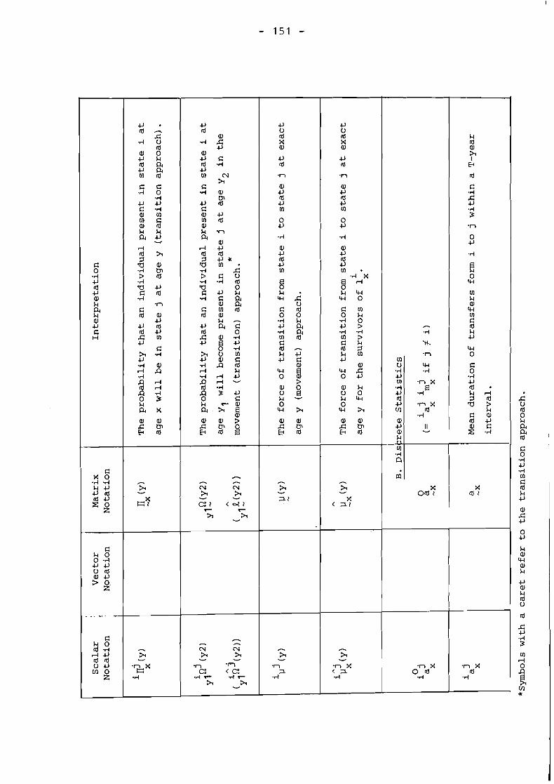
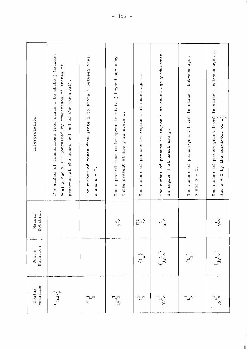
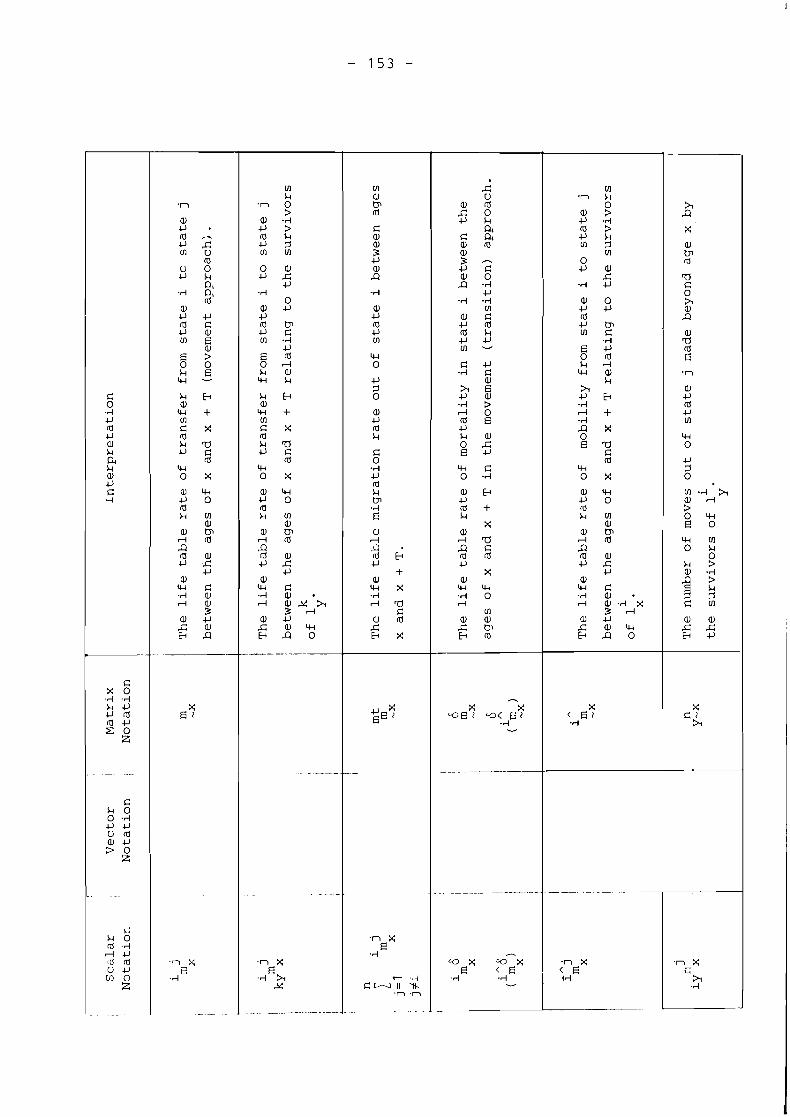

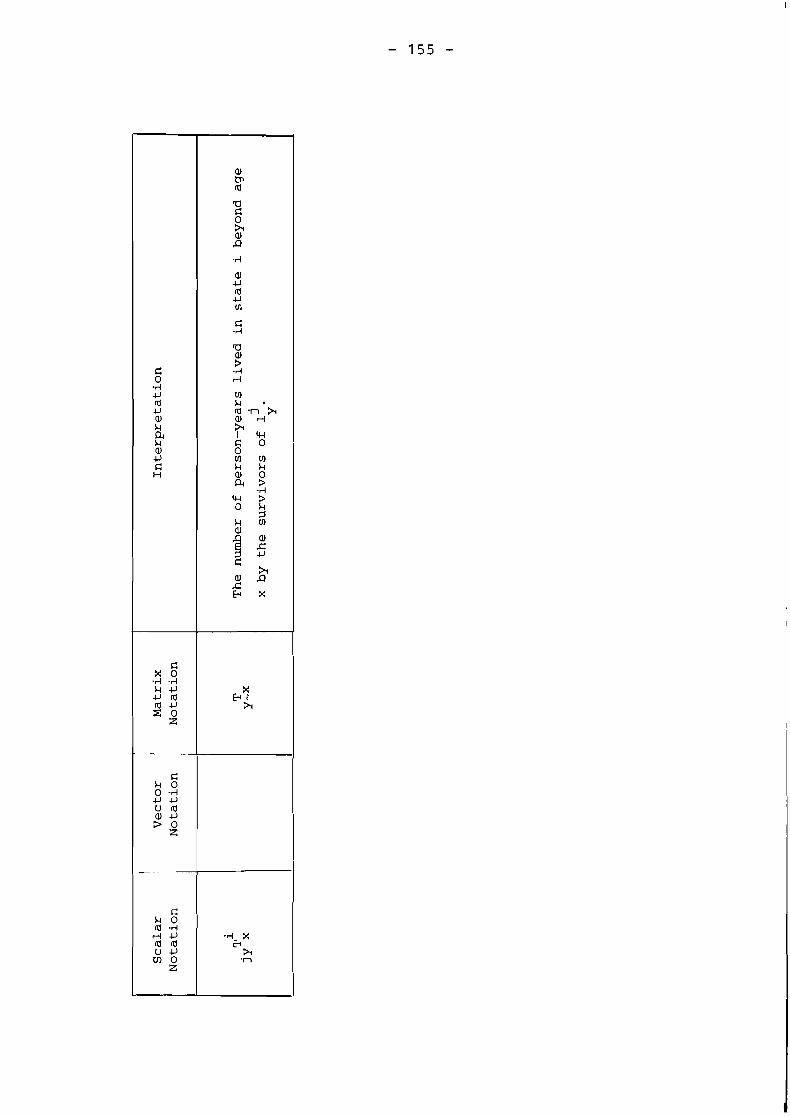
REFERENCES
Chiang, C.L. (1968), I n t r o d u c t i o n t o S t o c h a s t i c P r o c e s s e s i n B i o s t a t i s t i c s , Wiley, New York.
Cox, D.R., and H.D. Miller (1975), The Theory o f S t o c h a s t i c P r o c e s s e s , Wiley, Mew York.
Hoem, J.H. (1970), A Probabilistic Approach to Nuptiality, Biome t i - i e - p r a x i m e t r i e , 11, 3-1 9. -
Hoem, J.H. and M.S. Fong (1976), A Markov Chain Model o f Working L i f e Y'aDLes, WorKlng Paper # 2, Laboratory of Actuarial ~athematics, University of,Copenhagen.
Keyfitz, N. (1968), I n t r o d u c t i o n t o t h e Mathemat ics o f P o p u l a t i o n , Addison-Wesley, Reading, Mass.
Keyfitz, N. and J. Frauenthal (1975), An Improved ~ i f e Table Plethod, Biometz~ics, Vol . 3 1 , 889-899.
Krishnamoorthy, S. (1977), I nc remen t -dec remen t L i f e T a b l e s : a l ' l ; eo r t? t i ca l E x p o s i t i o n , an Improved ~ s t i m u t e and an A p p l i c a - t i o n , (unpublished manuscript) .
Ledent, J. (1972), On t h e L i f e T a b l e and S t a b l e Growth o f a Mu1 t i r e g iona L P o p u l a t i o n E x p e r i e n c i n g I n t e r n a l M i g r a t i o n , (unpublished masters thesis), Department of Civil Enqineeri~q ,
Northwestern University, Evanston, Ill.
Ledent, J., and Andrei Rogers (1972), An Interpolative-~terative Procedure for Constructing a Multiregional Life Table, M1.i 2 t i r e g - i o n a l Growth Node 2s P r o j e c t W P 9 / 7 2 , The Technological Institute, Northwestern University, Evanston, Ill.
Oechsli, F.W. (1972), The P u r i t y and N u p t i a l i t y Problem i n Demo- , j r d ( ~ p l ~ y , (unpublished Ph. D. dissertation) , Graduate Division, University of California, Berkeley.
Oechsli, F.W. (1975), A Population Model Based on a Life Table 'I'hat Includes Marriage and Parity, T h e o r e t i c a l P o p u l a t i o n 2 , - 7, 229-245.
Rogers, A. (1 973a) , Tlle rlultireqional Life Table, Journa l of j l ( l t Jl ;,, i~rt ic;.ul Soc ioZog; / , 3, 127-1 37. -
Roqers, A. (1973h), The Mathemtics of Multiregiona.1 nemagra~hic c;rc>wtll, i : ' t i z ) i i ionment arid PZ.alzn i r i y , 5, 3-29. -
. . - - !?ocjer:;, A. ('1 975a) , I l z5m due tiolz to Mul tir_o::::onal Ma thematied
. , l t , ~ ! i , . l g ~ ~ ; ~ ~ ~ i ~ ! j , Wiley , EJew York.
R o c j e ~ : ; , A. (1975b), Spatial Miy22trtwn Expectancies - RM 75-57 - I rite~rlat ional Institute for Applied Systems ~nalysis, l.axenburg, Austria.
Rogers, A., and J. Ledent (1974), Multiregional Population Pro- jection, Discussion paper No. 128, The Center for Mathematical Studies in Economics and Management Science - Northwestern University, Evanston, Ill., published in O p t i m i z a t i o n Tech - n i q u e s : Mode l ing and O p t i m i z a t i o n i n t h e S e r v i c e o f Man - P a r t I , ed. Jean Cea, Springer Verlag, Berlin 1976, 31-58.
Rogers, A., and J. Ledent (1976), Increment-Decrement ~ i f e Tables: A Comment, Demography, 13,2, 287-290-
Rogers, A., and J. Ledent (1977), Increment-Decrement Life Tables: Rejoinder, Demography, 14,4, 593.
Rogers, A., and B. Von Rabenau (1971), Estimation of Interregional Migration Streams from Place of Birth by Residence Data, Demography, - 8, 185-194.
Schoen, R. (1975), Constructing Increment-Decrement Life Tables, Demography, 12,2, 313-324
Schoen, R. (1977), Increment-Decrement Life Tables: Further Reactions to Rogers' and Ledent's C.omrnent, Demography, 14,4, 591-592
Schoen, R., and K.C. Land (1976), Finding Probabilities in Increment-Decrement Life Tables: A Markov Process Inter- pretation, WP 7603, Program i n A p p l i e d S o c i a l S t a t i s t i c s (PASS) - Department of Sociology, University of Illinois at Urbana-Champaign.
Schoen, R., and V.E. Nelson (1974), Marriage, Divorce and Mortality: A Life Table Analysis, Demography, - 11, 267-290.
PAPERS OF THE PIIGRATION AND SETTLEMENT STUDY
A. Papers in the Dynamics Series
1 . Andrei Rogers and Frans Willekens, Spatial Population Dynamics, RR-75-24, International Institute for Applied Systems Analysis, Laxenburq, Austria, 1975, published in papers, ~egionai Science Association, 36 (1976), 3-34.
2. Andrei Rogers and Jacques Ledent, llultiregional Popu- lation Projection, internal working paper, Inter- national Institute for Applied Systems Analysis, Laxenburg, Austria, published by Jean Cea, ed., Optimization Techniques: Modelling and Optimiza- tion in the Service of Man, Part 1, Springer Verlag, Berlin, 1976, pp. 31-58.
3. Andrei Rogers and Jacques Ledent, Increment-Decrement Life Tables: A Comment, internal working paper, ~nternational Institute for Applied Systems Analysis, Laxenburg, Austria, published in Demography, - 13 (1976), 287-290.
4. Andrei Rogers, Spatial Migration Expectancies, RM-75-57, International Institute for Applied Systems Analy- sis, Laxenburg, Austria, 1975.
5. Andrei Rogers, Aggregation and Decomposition in Popula- tion Projection, -. RM-76-11, International Institute for Applied Syst~~~ns Analysis, Laxenburg, Austria, ~)ublished in revised form in Environment and Planning A, - 8 (1976), 515-541.
6. A n d r e 1 Rogers and 1,uis J . Castro, Model Multiregional L ~ f e Tables and Stable - - Populations, RR-76-09, International Tric,titute for Applied Systems -
Ari.ilysis, Laxenbury, Austria, 1976.
1 . Ar~drei l<oyers and Frans ~~il lekens, Spatial Zero Popu- lation Growtli, RM-76-25, International Institute .-. -- - for Applied Systerlls Analysis, Laxenburg, Austria, 1976.
, . F r a n s Willekeris, - Sells1 - . - -- tlvity - - . p Analysis, RPI-76-49, Inter- national Institute for Applied Systems Analysis, Laxenbury, Austr~a, 1976, published in revised form in Envlron~i~:~~t - -- 41id - - Planning A, 9 (1977), - 653-674.

9. Andrei Rogers and Frans Willekens, The Spatial Repro- ductive Value and the Spatial Momentum of Zero Population Growth, RM-76-81, ~nternational Insti- tute for Applied Systems Analysis, Laxenburg, Austria, 1976.
10. Frans Willekens, The Spatial Reproductive Value: Theory and Applications, W-77-09, lnternzional Institute for ~ppl ied Systems Analysis, Laxenburg, Austria, 1977.
11. Michael A. Stoto, On the Relationship of Childhood to Labor Force Migration Rates, RM-77-55, Inter- national Institute for Applied Systems Analysis, Laxenburg, Austria, 1977.
Jacques Ledent, Intrinsic Rates and Stable ~ge-Specific Mortality (and Migration) Rates of the Growth fgion) ~oDulatikn Model, RM-77-37 j 1nte;nai tional Insti- tute for ~ ~ ~ 1 i e d ' S y s t e m s ~ n a l ~ s i s , Laxenburg, Austria, 1977.
13. Andrei Rogers, Richard Raquillet and Luis J. Castro, Model Migration Schedules and their Applications, RM-77-57, International Institute for ~ppl ied Systems Analysis, LaxenDurg, Austria, 1977.
14. Andrei Rogers, The Formal Demography of Migration and Redistribution: Measurement and ~ynamics, RM-78-15, - International Institute for Applied Systems Analysis, Laxenburg, Austria, 1978.
15 . Jacques Ledent, Some Methodological and Empirical Con- siderations in the - Construction of Increment-Decre- ment Life Tables, RM-78-00, International ~nstitute for Applied Systems Analysis, Laxenburg, Austria,
16. Jacques Ledent, Stable Growth in the Nonlinear Components- of-Change -- Model of Interregional P~pulation Growth and Distribution, RM-78-00, International Institute for Applied Systems Analysis, Laxenburg, Austria, 1978.
B. JJLipers in the Demometrics Series - -- I
1 . Altdrei Rogers, Demometrics of Migration and Settlement, RM-76-68, International Institute for Applied Systems Analysis, IJcixenburg, Austria, 1976, forth- coming in Papers of the Regional Science Association,
---. -- British Section, Pion Ltd., London. --
- . John Miron, Job-Search, Migration and Metropolitan - Growth, RM-77-03, International Institute for Applied Systems Analysis, Laxenburg, Austria, 1977.
. .iac:ques Ledent, Iiegional Multiplier Analysis: A Demo- -.---
metric Approach, -- RR-78-03, International Institute for Applied Systcrns Analysis, Laxenburg, Austria,l978.

C. Papers in the Policy Analysis Series
1. Yuri Evtushenko and Ross D. MacKinnon, Non-Linear Programming Approaches to National Settlement System planning, RR-77-26, International Institute for Applied Systems Analysis, Laxenburg, Austria, 1975, published in revised form in Environment and Planning A, 8 (1976), 637-653. -
2. R.K. Mehra, An Optimal Control Approach to National Settlement System Planning, RM-75-58, International Institute for Applied Systems Analysis, Laxenburg, Austria, 1975.
3. Frans Willekens, Optimal Migration Policies, RII-76-50, International ~nstitute for Applied Systems Analysis, Laxenburg, Austria, 1976.
4. Anatoli Propoi and Frans Willekens, A Dynamic Linear Programming Approach to National Settlement System Planning, RM-77-08, ~nternational Insti- tute for Applied Systems Analysis, Laxenburg, Austria, 1977.
5. Frans Willekens and Andrei Rogers, Normative Modeling in Demo-Economics, RR-77-23, International Insti- tute for Applied Systems Analysis, Laxenburg, Austria, 1977.
D. Papers in the Comparative Study Series
1. Ross D. MacKinnon and Anna Maria Skarke, Exploratorv Analyses of the 1966-1 971 ~ u s t r i a n - ~ i ~ k a t i o n Table, RR-75-31, International Institute for Applied Systems Analysis, Laxenburg, Austria, 1975, published in revised form in Regional Studies, 1 1 (1977), 99-111. -
2. Galina Kiseleva, The Influence of Urbanization on the Birthrate and Ilortalitv Rate for Maior Cities in the USSR, RM-75-68, ~ncernational Institute for Applied Systems Analysis, Laxenburg, Austria, 1975.
3. George Demko, Soviet Population Policy, RM-75-74, International Institute for Applied Systems Analysis, Laxenburg, Austria, 1975.
4. Andrei Rogers, The Comparative Pigration and Settlement Study: A Summary of Workshop Proceedinqs and ~onciusions, RM-76-0 1 , International Institute for Applied Systems Analysis, Laxenburg, Austria, 1976.
5. Andrei Rogers, Two Methodological Notes on Spatial Population Dynamics in the Soviet Union, RM-76-48, ~nkernationai Institute for Applied systems ~ n a l ~ s i s , Laxenburg, Austria, 1976.
6. Frans Willekens and Andrei Rogers, Computer Programs for Spatial Demographic Analysis, RM-76-58, International 1nstitut.e for Applied Systems - - - Analysis, Laxenburg, Austria, 1976.

7. Frans Willekens and Andrei Rogers, More Computer Pro- grams for Spatial Demographic Analysis, RM-77-30, International Institute for Applied Systems Analysis, Laxenburg, Austria, 1977.
8. Frans Willekens, The Recovery of Detailed Migration Patterns from Asaresate Data: An Ent rO~v Maxim.izina
2 2 2 L * 2
Approach, -- RM-77-58, International Institute for Applied Systems Analysis, Laxenburg, Austria, 1977.
. Related Papers of the Population, Resources and Growth Study
1. Nathan ~eyf i tz, Understanding World Models, RM-77-18, International Institute for Applied Systems Analysis, Laxenburg, Austria, 1977.
2. Andrei Rogers, Migration, Urbanization, Resources and Development, RR-77-41, International Institute for Applied Systems Analysis, Laxenburg, Austria, 1977.
3. Roman Kulikowski, Optimization of Rural-Urban Develop- ment - and Migration, - .- RM-77-41, International Institute for Applied Systems Analysis, Laxenburg, Austria, 1977.
4. Frans Willekens, Spatial PoF1lation Growth in Developing Countries: With a Special - -. - . .- - Emphasis on the Impacc of Agriculture, 1nternat:ional Institute for Applied Systems Analysis, Laxenburg, Austria, (forthcoming).
5. Henry Rernpel, The Role of Rural-Urban ~igrat ion in the - . - . --. .--.
urbanization and Econolnic Development Occurring in - - -. . - . - - -- . -- - . .. . -. - 7- Kcnya, RM-78-12, International ~nstitute for ~ ~ p l z e d - - . . . -. .- S y s tc~n~s Analysis, I,axt;~ll>ur:cj, Austria, 1978 .
6. A1 len C . Kelley and C. Swar t z , The Impact of Family Structure --- on %licroecononiic ~. . . Decision Makinq in De- \~c:Iopinq ~ Count-.ries : Kenya, International Institute A,-, For Applied System:-; <I .ysis , Laxenburg, Austria, ( fortlicc~ming) .