STATISTICAL AND METHODOLOGICAL CONSIDERATIONS FOR EXAMINING PROGRAM EFFECTIVENESS Carli Straight, PhD and Giovanni Sosa, PhD Chaffey College

RP Group Conference Presentation April 1, 2013

Pitfalls of Significance Testing

Assessment Item Number Correct

Pretest Number Correct

Posttest Statistically Significant?

Item 1 19 24 No

Item 2 12 16 No

Item 3 26 30 No

Item 4 7 10 No

Item 5 13 21 No

Item 6 5 13 No

Item 7 10 15 No

Item 8 6 16 No

Item 9 3 15 No

Avg. Correct 5.00 7.50 No

N = 30

Pitfalls of Significance Testing

NSSE Benchmark

Sample University N > 1000

Comparison Group N > 10,000

Statistically Significant?

Level of Academic Challenge

65.8 55.6 Yes

Active and Collaborative Learning

57.7 50.1 Yes

Student-Faculty Interaction

42.8 41.2 Yes

Enriching Educational Experiences

44.0 39.8 Yes

Supportive Campus Environment

62.7 56.9 Yes

Adapted from NSSE (2008)

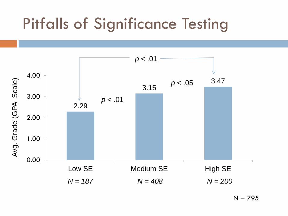
Pitfalls of Significance Testing

2.29

3.15 3.47

0.00

1.00

2.00

3.00

4.00

Low SE Medium SE High SE

N = 187 N = 408 N = 200

N = 795

Avg.

Gra

de (G

PA S

cale

)

p < .01

p < .05

p < .01

Significance Testing: Conclusions

P-values = Sample Size x Effect Size

Greatly influenced by sample size Do not speak to the magnitude of the difference Not well understood – even by ‘experts’

Practical Significance: Effect Size

Effect Size comes in various forms Standardized (d, r)

Cohen’s conventions:

d = .20 – small; .50 – moderate; .80 – large r = .10 – small; .30 – moderate; .50 - large

Discipline specific Aspirin Example (Rosenthal & Dimateo, 2002)

pooled

CT

sXXd −

=( ) ( )

211

21

22

12

−+−+−

=nn

nsnss ctpooled

Effect Size Examples

Assessment Item Number Correct

Pretest Number Correct

Posttest Statistically Significant?

Effect Size (d)

Item 1 19 24 No .37

Item 2 12 16 No .27

Item 3 26 30 No .75

Item 4 7 10 No .22

Item 5 13 21 No .55

Item 6 5 13 No .60

Item 7 10 15 No .34

Item 8 6 16 No .71

Item 9 3 15 No .93

Avg. Correct 5.00 7.50 No .61

N = 30

Effect Size Examples

NSSE Benchmark

Sample University N > 1000

Comparison Group

N > 10,000

Statistically Significant?

Effect Size (d)

Level of Academic Challenge

65.8 55.6 Yes .72

Active and Collaborative Learning

57.7 50.1 Yes .44

Student-Faculty Interaction

42.8 41.2 Yes .08

Enriching Educational Experiences

44.0 39.8 Yes .23

Supportive Campus Environment

62.7 56.9 Yes .30

Adapted from NSSE (2008)

Effect Size Examples

2.29

3.15 3.47

0.00

1.00

2.00

3.00

4.00

Low SE Medium SE High SE

N = 187 N = 408 N = 200

N = 795

Avg.

Gra

de (G

PA S

cale

)

d =.86

d = .35

d = 1.19

Wilson’s Effect Size Calculator

http://mason.gmu.edu/~dwilsonb/ma.html

Odds Ratios

Reflect a comparison of the relative odds of an occurrence of interest given the exposure to a variable of interest

OR = (A/B)/(C/D)

Successful Not

Successful Total

Medium SE 392 26 418

Low SE 145 52 197

OR = 15.077/2.788 = 5.40

Odds Ratios

Interpreting Odds Ratios: OR = 1.50 – small; 2.50 – moderate; 4.25 – large

OR = 1 => Intervention does not affect odds of outcome

OR > 1 => Intervention associated with higher odds of outcome

OR < 1 => Intervention associated with lower odds of outcome

Converting Odds Ratios to ds and vice versa:

[ ] 81.1ln ÷= ORd )*81.1( deOR =

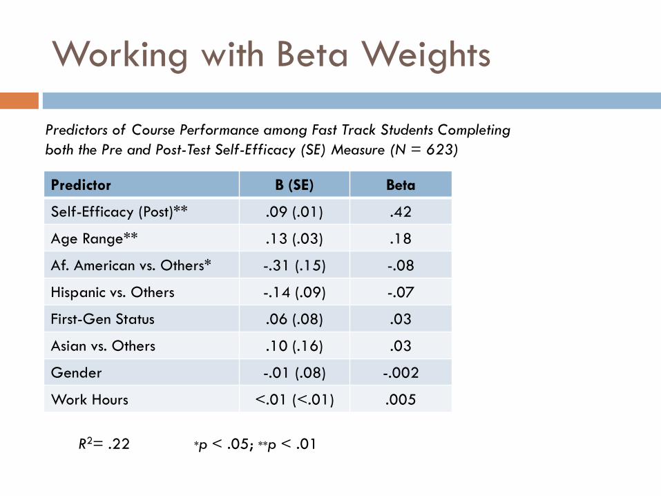
Working with Beta Weights

Predictor B (SE) Beta

Self-Efficacy (Post)** .09 (.01) .42

Age Range** .13 (.03) .18

Af. American vs. Others* -.31 (.15) -.08

Hispanic vs. Others -.14 (.09) -.07

First-Gen Status .06 (.08) .03

Asian vs. Others .10 (.16) .03

Gender -.01 (.08) -.002

Work Hours <.01 (<.01) .005

R2= .22 *p < .05; **p < .01

Predictors of Course Performance among Fast Track Students Completing both the Pre and Post-Test Self-Efficacy (SE) Measure (N = 623)

Working with Beta Weights

Predictor B (SE) Beta Zero-Order r Semi-Partial r Effect Size |d|

Self-Efficacy (Post)** .09 (.01) .42 .42 .41 .90

Age Range** .13 (.03) .18 .19 .18 .36

Af. American vs. Others*

-.31 (.15) -.08 -.05 -.07 .14

Hispanic vs. Others -.14 (.09) -.07 -.12 -.05 .10

First-Gen Status .06 (.08) .03 .05 .03 .05

Asian vs. Others .10 (.16) .03 .07 .02 .04

Gender -.01 (.08) -.002 -.11 -.002 .004

Work Hours <.01 (<.01) .005 .05 .005 .01

Predictors of Course Performance among Fast Track Students Completing both the Pre and Post-Test Self-Efficacy (SE) Measure (N = 623)

R2= .22 *p < .05; **p < .01

Basic Steps to Designing a Study that Measures Program Effectiveness

Example: How Do Students Perform in Fast-Track Courses? Select a reference point

Compared to whom/what?

Define what is meant by performance Course completion rate? Course success rate? Retention rate? Other?

Select appropriate statistical analysis Conduct analyses and write up results

Select Comparable Cohorts

Determine what/whom performance outcomes will be measured against

Goal is to select two cohorts that are the same in as many

ways as possible, minus participation in the relevant program Within-Group – observe outcomes of same students in program

and out of program (no need for controls) Between-Group – observe outcomes of different students, some of

whom participated in the program and some of whom did not (control for pre-existing group differences)

Select Comparable Cohorts

Within group comparisons Same students, compare performance in Fast-Track and non-Fast-Track

courses during same time period “Do students who earn GORs in both Fast-Track and non-Fast-Track

courses perform better, worse, or the same in the two formats?”

Between group comparisons Different students, one cohort earned a GOR in at least one Fast-Track

course and one cohort earned no GORs in a Fast-Track course across the same time period

“Do students who earn GORs in Fast-Track courses perform better, worse, or the same as students who do not earn GORs in Fast-Track courses?”

Select variables to control so that “all else is equal”

Within-Group Comparisons

1) Determine time period of interest Ensure that there are enough data to make comparisons

and that programmatic changes were not implemented during the selected period

Chaffey fast-track example: Fast-track courses were first implemented in spring 2010, but

significantly increased starting fall 2011 To obtain a strong sample size and ensure that some of the kinks

were worked out, data were analyzed from fall 2011 and later Using MIS referential files, select for fall 2011 and spring 2012

terms

Within-Group Comparisons

2) Code your data file so that student behavior in and out of the program can be measured

Chaffey fast-track example: Obtain a list of all fast-track sections from course scheduler or

other party on campus

Use obtained list to flag all fast-track sections in MIS file

Search start and end dates and delete short-term sections from file (use xf02 “SESSION-DATE-BEGINNING” and xf03 “SESSION-DATE-ENDING”)

Within-Group Comparisons

Delete all cases in which a student did not earn a GOR in fall 2011 or spring 2012

Create coding system for fast-track and full-term sections (e.g., compute two new variables, fast-track = 1 if section is fast-track and full-term = 1 if section is full-term)

Aggregate number of fast-track sections and number of full-term sections by student id and term (this will give you two new variables in your dataset that reflect a count of GORs each student earned in fast-track and full-term courses for each semester)

Within-Group Comparisons

3) Select for students whose behavior reflects program participation and program non-participation across the selected time period

Chaffey fast-track example: Select cases in which the sum of fast-track GORs >= 1 and the sum

of full-term GORs >= 1 (i.e., student has taken at least one fast-track and one full-term course)

Save selected cases to a new file

Within-Group Comparisons

4) Compare performance outcomes of same students in program and out of program

77.4%

70.0% 71.3%

65.0%

70.0%

75.0%

80.0%

Fast-Track GORs

Full-Term GORs

All Fall 2011 GORs

d = .17

d = .03

d = .14

N = 55,368 N = 4,546 N = 4,153

Same students All College

Succ

ess R

ate

Between-Group Comparisons

1) Determine time period of interest Ensure that there are enough data to make comparisons

and that programmatic changes were not implemented during the selected period

Chaffey fast-track example: Fast-track courses were first implemented in spring 2010, but

significantly increased starting fall 2011 To obtain a strong sample size and ensure that some of the kinks

were worked out, data were analyzed from fall 2011 and later Using MIS referential files, select for fall 2011 and spring 2012

terms

Between-Group Comparisons

2) Code data file so that two distinct cohorts, one of which participated in the program and one of which did not participate in the program, are identified

Chaffey fast-track example: Obtain a list of all fast-track sections from course scheduler or

other party on campus

Use obtained list to flag all fast-track sections in MIS file

Aggregate number of fast-track sections by student id and term (this will give you a new variable in your dataset that reflects a count of GORs each student earned in fast-track courses for each semester)

Between-Group Comparisons

Remove all records in which a GOR was not assigned

Create cohort variable with two mutually exclusive groups Cohort 1 consists of anyone who earned a GOR in a fast-track course

during the specified term (i.e., fast-track variable >= 1)

Cohort 2 consists of anyone who earned a GOR in a course or courses other than fast-track during the specified term (i.e., fast-track variable = 0)

Between-Group Comparisons

3) Compare cohort groups on a variety of pre-existing variables to measure differences outside of program participation (these will guide you in setting up controls for the next step)

Chaffey fast-track example: Gender, Ethnicity, Age, DPS Status, Enrollment Status, Academically

Disadvantaged Status, First Generation Status, Term Units Attempted, Term Units Earned, Cumulative Units Attempted, Cumulative Units Earned, Cumulative GPA, Self-Efficacy, Assessment Scores

Example of Categorical Variable Comparisons

Background Characteristics

Fast-Track Students Non-Fast-Track Students

|d| n % n %

Gender

Female 1,402 51.9 9,560 57.1 .10

Male 1,174 43.5 6,575 39.3 .09

Unknown 123 4.6 597 3.6 .05

First Generation

Yes 596 26.3 4,007 28.1 .27

No 1,669 73.7 10,264 71.9

Example of Continuous Variable Comparisons

Academic Characteristics

Fast-Track Students (n = 2,699)

Non-Fast-Track Students (n = 16,732)

|d| M SD M SD

Term Units Att 10.08 4.61 8.50 4.33 .36

Term Units Earn 7.21 4.89 5.79 4.59 .31

Cum Units Att 31.41 26.91 31.80 27.98 .01

Cum Units Earn 28.26 24.95 28.77 26.69 .02

Cum GPA* 2.57 1.04 2.42 1.12 .14

Self-Efficacy** 5.98 .83 5.93 .84 .06

*Fast-Track Students n = 2,689, Non-Fast-Track Students n = 16,643 ** Fast-Track Students n = 1,565, Non-Fast-Track Students n = 9,408

Between-Group Comparisons

4) Note where non-programmatic differences exist between cohort 1 and cohort 2, if observed

Chaffey fast-track example: Selecting for differences of d = .25 or higher, fast-track and non-

fast-track students were different in three areas: first-generation college status, term units attempted, and term units earned

Between-Group Comparisons

5) Conduct analyses to compare cohort 1 and cohort 2 performance outcomes, controlling for observed pre-existing differences between groups

Chaffey fast-track example: Calculate a partial correlation to measure the relationship

between cohort group and course success, while “controlling” for the effects of first generation status and units attempted (not units completed because it is too highly correlated with units attempted)

Between-Group Comparisons

Zero-Order r Partial r Effect Size

|d|

Cohort Group .01 .00 .02

Term Units Attempted* .06 .00 .12

First-Generation Status* -.03 -.03 .06

*p < .01

Correlates of Course Success among Students Earning a GOR in Fall 2011 (N = 19,431)

Cohort Comparison Conclusions

Students who earned at least one GOR each in fast-track and full-term courses in fall 2011 demonstrated statistically significantly higher course success rates in fast-track courses than in full-term courses. These findings, however, were not determined to be practically significant because of the large sample sizes and small effect size values.

Students who earned at least one GOR in a fast-track course in fall 2011 demonstrated course success rates that were not statistically significantly or practically different from course success rates of students who did not earn any GORs in fast-track courses in fall 2011.