Some Benchmark Simulations for Flash Flood Modelling E. Holzbecher, A. Hadidi Department of Applied Geosciences, German University of Technology in Oman, Muscat, Oman Introduction Flash floods are sudden and mostly destructive rushes of water down narrow gullies or over sloping surfaces. They are mostly caused by heavy rainfall in the upstream watershed. They may also appear as result of catastrophic events as dam or levee breaks, mudslides or debris flow. The occurrence of flash floods is determined by many factors, like intensity, location and distribution of the rainfall, topography, land use and vegetation cover, soil type, and soil saturation. These factors determine the spatial and temporal development of a flood. Urban areas are also prone to flash floods, because impervious surfaces prevent water to infiltrate into the ground. Moreover damages are more severe in highly populated areas than in the remote countryside. The simulation of flash floods has thus become a tool that is increasingly used. One application area is urban planning. In general flood modelling is utilized to delineate flood risk maps. Moreover such tools are applied in early warning systems, in order to predict the rush of a fluid front as reaction of a certain rainfall event. Modelling Approaches Most modellers prefer the 2D depth averaged formulation in flash flood simulations in contrast to the general 3D formulation. The 2D version definitely has advantages concerning the general formulation with respect to computer resources. Near the fluid front mesh refinement is required, which highly increases the computational cost of 3D models. The 2D approach leads to the shallow water equations (SWE), also known as Saint-Venant equations. Vertical velocities are usually much smaller than horizontal components, and are thus neglected. SWE consists of three coupled differential equations, one for the height of the water column and two for the mean horizontal velocity components. The system can be implemented in COMSOL Multiphysics using pde-modes. We utilized a physics

mode for the SWE (Schlegel 2012). The SWE can be written as:

∂η∂t

+∇⋅ Hu( ) = 0 (1)

∂u∂t

+ u ⋅∇( )u+ g∇H −F = 0 (2)

with total water depth H, water height above reference height η, velocity vector u, acceleration and due to gravity g (Takase et al. 2010). In the vector F the contributions of all other forces are gathered. The equations are derived from the volume and momentum conservation principles, formulated on depth-averaged variables. The derivation is based on several assumptions: the fluid is incompressible, in the vertical direction there is hydrostatic pressure distribution, depth-averaged values can be used for all properties and variables, the bottom slopes are small, there are no density effects from variable fluid density or fluid viscosity, the eddy viscosity is much larger than molecular viscosity, atmospheric pressure gradient can be ignored, etc. The system of equations (1) and (2) is nonlinear. Friction at the walls, i.e. at the interfaces between fluid and solid, can be taken into account by an additional term in equation (2) (Brufau & García-Navarro 2000, Duran 2015):

∂u∂t

+ u ⋅∇( )u+ g∇H + gηn2 uη4/3 u−F = 0 (3)

with Manning coefficient n. Heniche et al. (2000) add another term to consider the influence of wind speed at the surface of the shallow water body. In this work we focus on the original form, i.e. equation (2). Some test runs with equation (3) showed no relevance of friction for the considered test cases. Wind speed effects are neglected, as they are likely to be irrelevant in highly dynamic dam break scenarios. It is well-known that the solution of the SWEs (1)(2) may suffer from severe instabilities. Straightforward modelling, either using finite differences or finite element techniques, leads to spurious oscillations. For that reason various stabilization schemes have been proposed. The most basic method is the introduction of an artificial viscosity, which appears

Excerpt from the Proceedings of the 2017 COMSOL Conference in Rotterdam

in an additional term on the left side of equations (2) (Chen et al. 2013):

∂u∂t

+ u ⋅∇( )u+ g∇H −ν∇2u−F = 0 (4)

with artificial viscosity ν. This is done in analogy with stabilisation methods for the advection-diffusion equation, where similar numerical problems arise simulating almost sharp chemical or thermal fronts. The method of artificial viscosity successfully stabilizes the solution and prevents oscillatory errors. However this method introduces a numerical diffusion, which is not presented in the original equations and in real systems. Gradients are smoothed, but without physical justification, i.e. the method is inconsistent. Consistent stabilization methods have been derived.

1D Dambreak Benchmark Dam break models that are used for benchmarking, are based on a highly simplified concept of a real dam break. The breaking wall itself does not appear in the simple setting. The simulation starts at time t=0 with the steep step of the water table at the interface between the reservoir and backwater region. Starting from this highly idealized step situation models based on the SWE simulate the development of the water table for t>0. The simple set-up includes two water heights: one higher value for the reservoir (h1) and a lower (h0) for the backwater. These two values, together with the parts of the model region in which they prevail, constitute the initial condition. In a 1D model the interface between reservoir and backwater is just the position x0, at which the dam and thus the initial water table jump is located; see the sketch in Figure 1. With this the physical parameters of the classical 1D dam break problem are completed.

Figure 1. Sketch of 1D dam break model, showing initial conditions and terminology

A fact that makes the dam break problem attractive as a benchmark is that an analytical solution exists. For the given setting an analytical solution has been provided by Stoker (1957), which we will utilize below. It consists mainly of two waves (of different kind), one moving into the reservoir and one into the backwater region.

Figure 2. Sketch of the analytical solution for the 1D dam break model in the x-t diagram If not mentioned otherwise we report results on the reference case described above with parameter values h1=2 m and h0=1 m. Model region is the unit length interval x ∈ 0,1⎡⎣ ⎤⎦ m with dam break position at

x0=0.5 m. The first examples highlight the numerical problems involved with the solution of the nonlinear SWE. Straight forward implementation of standard numerical methods without any stabilization leads to inacceptable oscillations, as illustrated in Figure 3a, showing initial and simulated water tables at selected times after dam break. The problem of spurious oscillations was reported already in the early days of numerical modeling. The well-known problem of spurious oscillations can be resolved by using an artificial viscosity to stabilize the solution. However, this solution is inconsistent. It leads to a numerical diffusion, which is smoothing all gradients. Thus sharp slopes become less steep, even at parts where steep gradients are physically correct. However there are consistent stabilization methods, as outlined above, which avoid the global smoothing. Figure 3b illustrates the effect of numerical diffusion clearly. In the figure results are compared for inconsistent and consistent stabilization. For the latter we combined streamline diffusion and shock capturing stabilization.

Excerpt from the Proceedings of the 2017 COMSOL Conference in Rotterdam

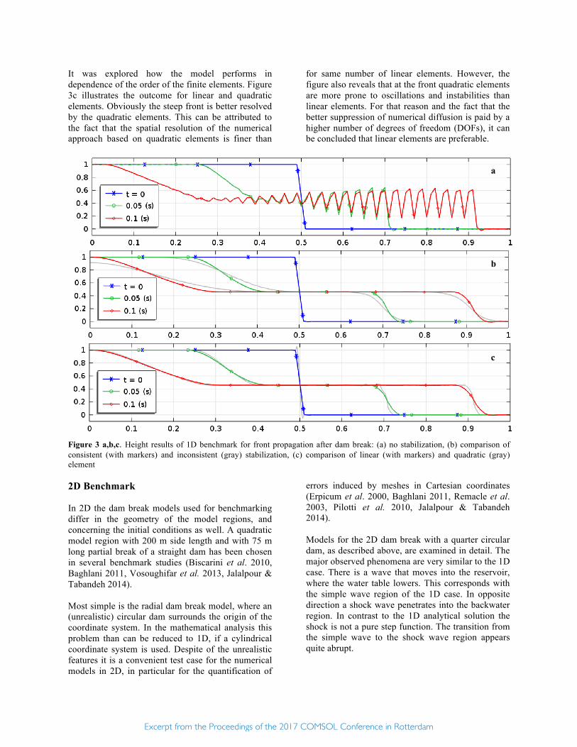
It was explored how the model performs in dependence of the order of the finite elements. Figure 3c illustrates the outcome for linear and quadratic elements. Obviously the steep front is better resolved by the quadratic elements. This can be attributed to the fact that the spatial resolution of the numerical approach based on quadratic elements is finer than

for same number of linear elements. However, the figure also reveals that at the front quadratic elements are more prone to oscillations and instabilities than linear elements. For that reason and the fact that the better suppression of numerical diffusion is paid by a higher number of degrees of freedom (DOFs), it can be concluded that linear elements are preferable.

Figure 3 a,b,c. Height results of 1D benchmark for front propagation after dam break: (a) no stabilization, (b) comparison of consistent (with markers) and inconsistent (gray) stabilization, (c) comparison of linear (with markers) and quadratic (gray) element 2D Benchmark In 2D the dam break models used for benchmarking differ in the geometry of the model regions, and concerning the initial conditions as well. A quadratic model region with 200 m side length and with 75 m long partial break of a straight dam has been chosen in several benchmark studies (Biscarini et al. 2010, Baghlani 2011, Vosoughifar et al. 2013, Jalalpour & Tabandeh 2014). Most simple is the radial dam break model, where an (unrealistic) circular dam surrounds the origin of the coordinate system. In the mathematical analysis this problem than can be reduced to 1D, if a cylindrical coordinate system is used. Despite of the unrealistic features it is a convenient test case for the numerical models in 2D, in particular for the quantification of

errors induced by meshes in Cartesian coordinates (Erpicum et al. 2000, Baghlani 2011, Remacle et al. 2003, Pilotti et al. 2010, Jalalpour & Tabandeh 2014). Models for the 2D dam break with a quarter circular dam, as described above, are examined in detail. The major observed phenomena are very similar to the 1D case. There is a wave that moves into the reservoir, where the water table lowers. This corresponds with the simple wave region of the 1D case. In opposite direction a shock wave penetrates into the backwater region. In contrast to the 1D analytical solution the shock is not a pure step function. The transition from the simple wave to the shock wave region appears quite abrupt.

a

b

c

Excerpt from the Proceedings of the 2017 COMSOL Conference in Rotterdam

For error investigations we examine the 2D solutions along the two diagonals of the model region. Along the main diagonal one can observe the longitudinal wave movement. However, when the model is run without any stabilization spurious oscillations dominate the picture, as demonstrated in Figure 9a. As in the 1D benchmark these results are clearly unacceptable. Using stabilization techniques the movement of the wave can be simulated. That is demonstrated in in Figure 9b, where the results with inconsistent and consistent stabilization can be compared. Clearly the inconsistent method introduces numerical diffusion, which makes this method unacceptable as well. As consistent stabilization methods we used streamline diffusion and shock capturing.

For the consistent stabilization techniques Figure 9c shows the effect of two mesh refinements on the front development in longitudinal direction. The effect of mesh refinement is a steepening of the fronts, which is effective on the left side, at the transition between simple wave and shock wave regime and most clearly at the front of the shock wave. Higher accuracy was achieved at the cost of increased computer resources. The reference mesh has 7803 DOF and the simulation took 43 s execution time. The refined model needed considerably more computer resources: 30603 DOF and 10:23 min execution time. The double refined mesh has 121203 DOF and needed 1 h 23:41 min for execution.

Figure 4 a,b,c. Front propagation after dam break (2D) along the main diagonal at selected time instances: (a) no stabilization, (b) comparison of solutions obtained with consistent and inconsistent stabilization, (c) comparison of results with consistent stabilization with two grid refinements: reference mesh (gray), refined mesh (spacing 0.01 m, black), and double refined mesh (spacing 0.005 m, color)

a

b

c

Excerpt from the Proceedings of the 2017 COMSOL Conference in Rotterdam

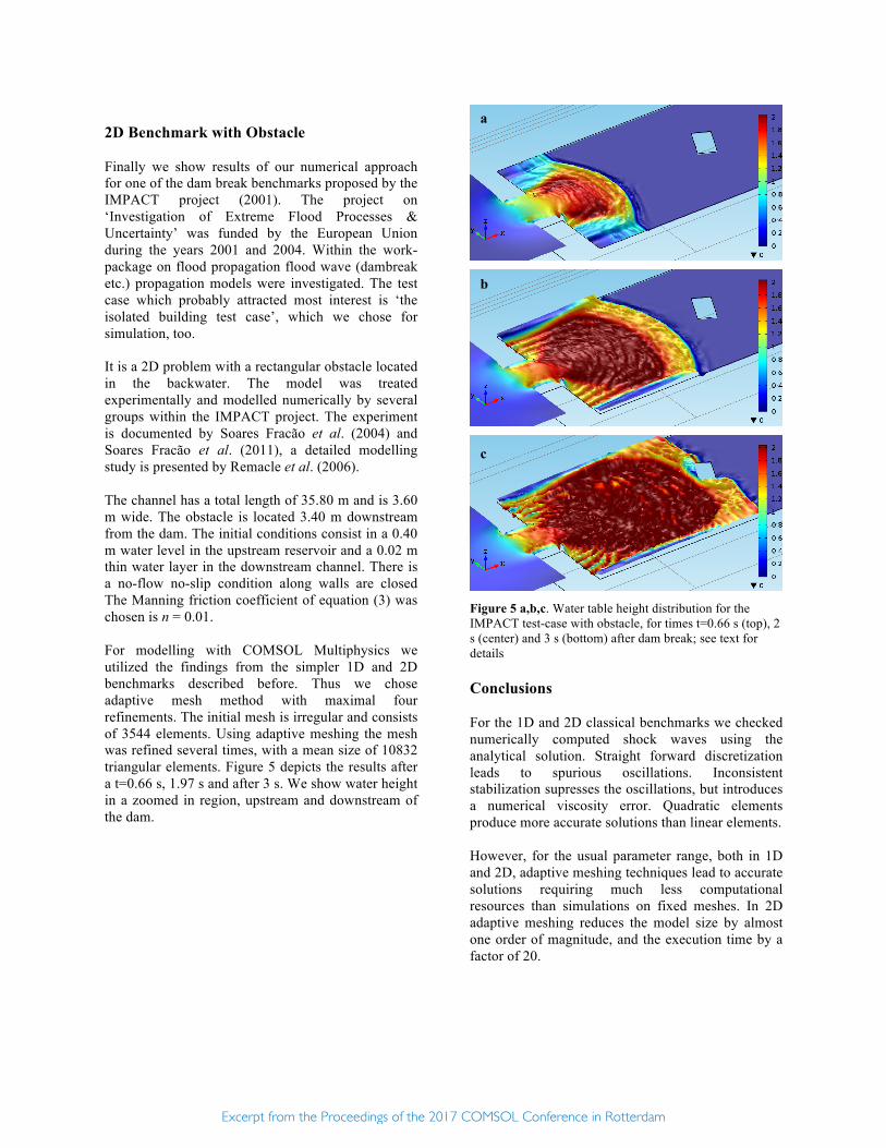
2D Benchmark with Obstacle Finally we show results of our numerical approach for one of the dam break benchmarks proposed by the IMPACT project (2001). The project on ‘Investigation of Extreme Flood Processes & Uncertainty’ was funded by the European Union during the years 2001 and 2004. Within the work-package on flood propagation flood wave (dambreak etc.) propagation models were investigated. The test case which probably attracted most interest is ‘the isolated building test case’, which we chose for simulation, too. It is a 2D problem with a rectangular obstacle located in the backwater. The model was treated experimentally and modelled numerically by several groups within the IMPACT project. The experiment is documented by Soares Fracão et al. (2004) and Soares Fracão et al. (2011), a detailed modelling study is presented by Remacle et al. (2006). The channel has a total length of 35.80 m and is 3.60 m wide. The obstacle is located 3.40 m downstream from the dam. The initial conditions consist in a 0.40 m water level in the upstream reservoir and a 0.02 m thin water layer in the downstream channel. There is a no-flow no-slip condition along walls are closed The Manning friction coefficient of equation (3) was chosen is n = 0.01. For modelling with COMSOL Multiphysics we utilized the findings from the simpler 1D and 2D benchmarks described before. Thus we chose adaptive mesh method with maximal four refinements. The initial mesh is irregular and consists of 3544 elements. Using adaptive meshing the mesh was refined several times, with a mean size of 10832 triangular elements. Figure 5 depicts the results after a t=0.66 s, 1.97 s and after 3 s. We show water height in a zoomed in region, upstream and downstream of the dam.

Figure 5 a,b,c. Water table height distribution for the IMPACT test-case with obstacle, for times t=0.66 s (top), 2 s (center) and 3 s (bottom) after dam break; see text for details Conclusions For the 1D and 2D classical benchmarks we checked numerically computed shock waves using the analytical solution. Straight forward discretization leads to spurious oscillations. Inconsistent stabilization supresses the oscillations, but introduces a numerical viscosity error. Quadratic elements produce more accurate solutions than linear elements. However, for the usual parameter range, both in 1D and 2D, adaptive meshing techniques lead to accurate solutions requiring much less computational resources than simulations on fixed meshes. In 2D adaptive meshing reduces the model size by almost one order of magnitude, and the execution time by a factor of 20.

a

b

c

Excerpt from the Proceedings of the 2017 COMSOL Conference in Rotterdam

References

1. Baghlani A., Simulation of dam-break problem by a robust flux-vector splitting approach in Cartesian grid, Scientia Iranica A 18(5), 1061-1068 (2011) 2. Biscarini C., Di Francesco S., Manciola P., CFD modelling approach for dam break flow studies, Hydrol. Earth Syst. Sci. 14, 705–718 (2010) 3. Brufau P., García-Navarro P., Two-dimensional dam break flow simulation, Int. J. Numer. Meth. in Fluids 33, 35–57 (2000) 4. Chen Y., Kurganov A., Lei M., Liu Y., An adaptive artificial viscosity method for the Saint-Venant system. In: Ansorge R. et al. (Eds.). Recent Developments in the Numerics of Nonlinear Conservation Laws, Vol. 120 of Notes on Numerical Fluid Mechanics and Multidisciplinary Design, Springer-Publ. Berlin: 125-141 (2013) 5. Duran A., A robust and well balanced scheme for the 2D Saint-Venant system on unstructured meshes with friction source term, Int. J. for Numer. Meth. in Fluids 78(2), 89-121 (2015) 6. Erpicum E., Dewals B.J., Archambeau P., Pirotton M., Dam break flow computation based on an efficient flux vector splitting, J. of Comp. and Appl. Math. 234, 2143–2151 (2010) 7. Heniche M., Secretan Y., Boudreau P., Leclerc M., A two-dimensional finite element drying-wetting shallow water model for rivers and estuaries. Adv. in Water Res. 23, 359-372 (2000) 8. IMPACT (2001), http://www.impact-project.net/impact_project_overview.htm 9. Jalalpour H., Tabandeh S.M., Effect of a high resolution finite volume scheme with unstructured Voronoi mesh for dam break simulation, J. of Civil Eng. and Urbanism 4(4), 474-479 (2014) 10. Pilotti M., Tomirotti M., Valerio G., Bacchi B., Simplified method for the characterization of the hydrograph following a sudden partial dam break. J. of Hydr. Eng. (ASCE) 136(10), 693-704 (2010) 11. Remacle J.-F., Soares Frazao S., Li X., Shephard M.S., An adaptive discretization of shallow-water equations based on discontinuous Galerkin methods. Int. J. Numer. Meth. Fluids 52(8), 903-923 (2006) 12. Schlegel F., Shallow water physics (shweq). COMSOL internal paper, private communication (2012) 13. Soares Frazão S., Noël B., Zech Y., Experiments of dam-break flow in the presence of obstacles. Proceedings of River Flow 2004, Naples, Italy (2004) 14. Soares Frazão S., Spinewine B., Zech Y., Dam-break wave against a skew obstacle, validation of voronoi particle tracking methods for velocity field

measurement. Experiments in Fluids 50(6), 1633-1649 (2011) 15. Stoker J.J., Water Waves, The Mathematical Theory with Applications, Interscience, London (1957) 16. Takase S., Kashiyama K., Tanaka S., Tezduyar T.E., Space-time SUPG finite element computation of shallow-water flows with moving shorelines, J. Comp. Mech. 48(3), 293-306 (2011) 17. Vosoughifar H.R., Dolatshah A., Shokouhi S.K.S., Discretization of multidimensional mathematical equations of dam break phenomena using a novel approach of finite volume method, J. of Appl. Math. 2013, 12p (2013)

.

Acknowledgements The presented research is enabled as part of the project funding from The Research Council (TRC) of the Sultanate of Oman under Research Agreement No. ORG/ GUTECH /EBR/13/026. Special thanks to the Ministry of Regional Municipal and Water Resources in Oman for providing observation data.

Excerpt from the Proceedings of the 2017 COMSOL Conference in Rotterdam