physical scale modelling of urban flood systemsetheses.whiterose.ac.uk/9270/1/phd thesis matteo...
TRANSCRIPT

1
Physical scale modelling of urban flood
systems
Research student: Matteo Rubinato
Supervisors: Dr J.Shucksmith
Prof. A.J.Saul
Department of Civil and Structural Engineering
University of Sheffield
Thesis Submitted in Partial Fulfilment of the
Requirements for the Degree of Doctor of Philosophy
Date: June 2015

2
ACKNOWLEDGEMENTS
The author would sincerely like to acknowledge the following individuals for their
professional support and friendship during the course of this PhD study and throughout
the author’s career at the University of Sheffield.
Professor Adrian Saul, for introducing me to the academic career through the PhD,
much valued advice and support that you have shown me throughout my career at the
University of Sheffield.
Lecturer Dr. James Shucksmith, for his admirable supervision and help through all the
process of the research undertaken.
Head of the Department Harm Askes, for his excellent care during critical moments due
to the lack of funding.
Finally to my family, Leonardo, Maria Grazia, Lara e Dario, thanks for believing I
could do it, thanks for accepting my decision to be far from home during these years to
reach this essential degree for my future career. You have been and you will always be
the most important people in my life, always there to support and help me when things
are both negative and positive. And thanks to my girlfriend Amandine, which has
always been there to give me positive support and advices.
3
ABSTRACT
Urban flooding is defined as ‘an overflowing or irruption of water over urban pathways
which are not usually submerged’. Current economic, climatic and social trends suggest
that the frequency, magnitude and cost of flooding are likely to increase in the future.
Hydraulic models are commonly used by engineers in order to predict and mitigate
flood risk. However full scale calibration and validation datasets for these modelling
tools are scarce.
The main research objective of this thesis was to design and construct a physical model
in order to provide datasets useful to verify, calibrate and validate computer model
results in terms of energy losses in manholes.
To address these issues, an experimental facility has been constructed to enable the
investigation of energy losses under steady and unsteady flow conditions in a scaled
sewer system. Originally the model was composed of six manholes and three main
pipes and then it was modified into a single pipe linked to an urban surface through a
single manhole.
Experiments involved the measurement of flow rates, velocity, pressure and water depth
within the physical models under different hydraulic scenarios.
Steady flow tests were conducted to quantify energy losses though manhole structures
with different inlet/outlet configurations under a range of hydraulic conditions.
Unsteady flow tests were conducted to examine the performance of different
computational hydraulic models. These tests have shown that the performance of the
SWMM hydraulic model could be improved by including local losses in the calibration
process.
After modification the model was used to quantify sewer to surface and surface to sewer
flow exchange through a single manhole during pluvial flooding. The work has
demonstrated the feasibility of using weir and orifice equations within modelling tools
to quantify this exchange under steady conditions. The model was used to empirically
quantify discharge coefficients for energy loss equations which describe flow exchange
for the first time.

4
CONTENTS
ACKNOWLEDGEMENTS .............................................................................................. 2
ABSTRACT ...................................................................................................................... 3
List of Figures ................................................................................................................... 6
List of Tables .................................................................................................................. 11
Notation list ..................................................................................................................... 13
1. INTRODUCTION ................................................................................................... 17
1.1. Aims of thesis ................................................................................................... 19
1.2. Thesis structure................................................................................................. 19
2 BACKGROUND – LITERATURE REVIEW ........................................................ 20
2.1 Urban flooding ................................................................................................. 20
2.1.1 Overview of urban flood modelling .......................................................... 22
2.2 Conservation of energy and head losses........................................................... 23
2.3 Head Losses within In line Manholes .............................................................. 25
2.3.1 Detail of Selected Previous Studies on In-line Manholes ......................... 27
2.4 Junction Manholes ............................................................................................ 28
2.4.1 Detail of selected experimental studies in junction manholes .................. 30
2.5 Summary .......................................................................................................... 38
2.6 Interaction of below/above ground flows and flow over the surface ............... 38
2.7 Application of exchange equations within urban flood models ....................... 43
2.8 Experimental quantification of flow exchange ................................................ 46
2.9 Existing limitations and gaps in flood modelling tools .................................... 48
2.10 Thesis objectives .............................................................................................. 49
3 METHODOLOGY .................................................................................................. 50
3.1 Scaling factors and similitudes ......................................................................... 50
3.2 Experimental facility (configuration 1) ............................................................ 53
3.3 Facility testing phase 2 ..................................................................................... 59
3.4 Managing and controlling the model (testing phase 1 and 2) .......................... 65
3.5 Instrumentation ................................................................................................. 69
3.5.1 Valves........................................................................................................ 69
3.5.2 Flow meters ............................................................................................... 70
3.5.3 Pressure transducers .................................................................................. 71
3.6 Calibration of Instrumentation ......................................................................... 72
3.6.1 Pressure sensor calibration ........................................................................ 72

5
3.6.2 Valve calibration ....................................................................................... 76
3.6.3 Error Analysis ........................................................................................... 81
4 Pipe Network Results............................................................................................... 84
4.1 Steady flow tests in the pipe network system ................................................... 84
4.2 Secondary losses ............................................................................................... 84
4.3 Head losses due to friction in pipes .................................................................. 90
4.4 “In line” manholes ............................................................................................ 93
4.5 Energy Losses Through Manholes with Multiple inlets................................... 95
4.6 Quantification of hydraulic capacity of the sewer system................................ 97
4.7 Scaled Rainfall Event Simulations ................................................................... 98
4.8 Scaling procedures for physical models ......................................................... 101
4.9 Comparison between computer modelling results in Infoworks and the
physical model results for flow ................................................................................. 103
4.10 Flow conditions at network junctions ............................................................ 107
4.11 Results and Discussion ................................................................................... 109
5 Results of above/below ground physical model .................................................... 115
5.1 Exchange below/above ground urban floods: steady flow conditions .......... 115
5.1.1 Scenario 1 ................................................................................................ 116
5.1.2 Scenario 2: Outflow with urban surface flow ......................................... 120
5.1.3 Scenario 3: Outflow with interaction of shallow water in the urban surface
122
6 Conclusions ............................................................................................................ 125
7 Further work .......................................................................................................... 127
8 References .............................................................................................................. 131
9 Appendix A ............................................................................................................ 138
List of journal papers published .................................................................................... 159
List of journal papers under review .............................................................................. 159
List of journal papers in progress .................................................................................. 159
List of conference papers published .............................................................................. 159

6
List of Figures
Figure 1 - Carlisle, England, 2005 (Image source: Wikimedia Commons) .................... 17
Figure 2 – Examples of system surcharge and exceedance flow generation. Left) Central
Texas, Herald/TJ MAXWELL, Right) Waynesville, Aug. 9, 2013 Steve
Zumwalt/FEMA .............................................................................................................. 20
Figure 3 – General Urban Flood Events, 1970-2011. Source: EM-DAT: The
OFDA/CRED International Disaster Database www.emdat.be – Universite’ Catholique
de Louvain – Brussels, Belgium (Jha et al, 2011). ......................................................... 21
Figure 4 – Pressurized flow with associated energy grade lines and hydraulic grade lines
(Asztely, 1995). ............................................................................................................... 24
Figure 5 – Elevations of typical manholes (surcharged condition) - Asztely (1995). .... 25
Figure 6– Head losses for a multiple inlet manhole. ....................................................... 28
Figure 7 - Experimental setup of a 90° sewer junction (Zhao et al., 2006). ................... 32
Figure 8 – Plan view of the 25.8 Edworthy model junction (Zhao et al., 2006). ............ 32
Figure 9 – Energy loss coefficients for pressurized flow pipe in the 25.8 degrees
Edworthy junction of a) K13; b) K23; and c) K measurements with half benching (filled
square), without benching (empty square) and predictions of Equation 9 and 10 (straight
line) [Zhao et al., (2006)]. ............................................................................................... 33
Figure 10 - Energy loss coefficients for pressurized flow pipe in the 90 degrees junction
of a) K13; b) K23; and c) K measurements Zhao et al., (2006) Q3 = 0.90 (empty triangle),
Q3=1.35 (cross) and Q3=1.79 (empty circle) with So=0 and Q3 =1.79 (filled square) with
So=0.061. Results of Wang et al (1998) (filled circle), Marsalek (1985), no benching
(dash line with empty circle), half benching (dash line with empty square), full benching
(dash line with empty triangle) and predictions of Equation 9 and 10 (straight line)
[Zhao et al., (2006)]. ....................................................................................................... 33
Figure 11 – Experimental apparatus (on the right), crown alignment (a), center
alignment (b) and perpendicular connection between inflow and outflow pipes (c) (Arao
et al., 2012)...................................................................................................................... 35
Figure 12 – The model of the junction with the correspondent possible variations of the
model itself (Saldarriaga et al., 2012). ............................................................................ 36
Figure 13 – Scheme of the junction manhole: (a) plan view for 45 º, (b) plan view for 90
º (c) section and overview of the model including jet boxes, conduits and junction,
(Pfister and Gisonni, 2014). ............................................................................................ 37
Figure 14 – Examples of rectangular (left) and Cipoletti (right) weirs. ......................... 39
Figure 15 – General any shape notch. ............................................................................. 39
Figure 16 – Rectangular weir scheme. ............................................................................ 40
Figure 17 – Bottom discharge and side discharge. ......................................................... 40
Figure 18 – Free weir linkages. ....................................................................................... 43
Figure 19 – Submerged weir linkage. ............................................................................. 44
Figure 20 – Orifice linkage. ............................................................................................ 45
Figure 21 – Experimental setup used for this study (Djordjevic et al., 2013). ............... 46
Figure 22 – Top view and cross section view of the experimental facility developed by
Bazin et al., 2014. GR corresponds to the street inlet grid, DB is the drainage box, DT
the drainage tube and DP the drainage pipe. ................................................................... 47
7
Figure 23 - Examples of scaled pipes on the left (a) and junction manhole on the right
(b). ................................................................................................................................... 53
Figure 24 - Scheme of system inherited from D. Unwin with manhole labels (Mx). ..... 54
Figure 25 - Main pipe (branch A) First manhole (downstream view) ............................ 54
Figure 26 - Main pipe (branch A) Third manhole (downstream view)........................... 55
Figure 27 - Branch “C” (upstream view) ........................................................................ 55
Figure 28 - Birdseye view of the whole system prior the construction of the urban
surface (from “upstream”)............................................................................................... 56
Figure 29 – Tank receiving outlet’s flow and combined sewer overflow....................... 56
Figure 30 – Downstream view of the two re-circulating water tanks underneath the pipe
system. ............................................................................................................................. 57
Figure 31 – Particular detail of the pump (left) used to fill the three feeding tanks
(right)............................................................................................................................... 57
Figure 32 – Particular detail of the three tanks being filled with water. ......................... 58
Figure 33 – Full view of the new inlet system. .............................................................. 58
Figure 34– Connection between header tank and the three inlet pipes plus the inlet of
the urban surface. ............................................................................................................ 59
Figure 35 – Initial elevation above datum (in mm) of the system divided in a grid 1 m x
1 m ................................................................................................................................... 60
Figure 36 – Plan view of the urban surface. ................................................................... 61
Figure 37 –Location of the pressure measurement points (distances in mm) on the urban
surface around the manhole. ........................................................................................... 61
Figure 38 –Plan view of the pressure measurement points (Px) on the urban surface
around the manhole. ........................................................................................................ 62
Figure 39 –Material inserted in the inlet tank (Left). Inlet Weir (Right). ....................... 63
Figure 40 – Longitudinal profile of the physical model used in phase 2. ....................... 63
Figure 41- Urban surface: on the left view from the upstream, on the right view from the
downstream. .................................................................................................................... 64
Figure 42 – Instrumentation scheme on the pipe network (phase 1 setup). .................... 65
Figure 43– Front panel of the interface developed. ........................................................ 67
Figure 44- Block diagram of the interface developed. .................................................... 68
Figure 45 – Valve and DPS. ............................................................................................ 69
Figure 46- How an Electromagnetic Flow meter MAG 900 works and real example ... 70
Figure 47 - Suggested location for Mag Flow Meters (MAG Flow Meter, Installation
Manual, Ver.2001-1). ...................................................................................................... 71
Figure 48 - “T” connection utilized for pipe downstream urban surface as well as sewer
system. ............................................................................................................................. 71
Figure 49 – Pressure transducers GEMS ........................................................................ 72
Figure 50 – Description of the process to find the relationship depth of water vs output
in Ampere ........................................................................................................................ 73
Figure 51 – Equipment for calibration of the pressure sensors for the urban surface. ... 74
Figure 53 - Calibration pressure sensor P M Up vs water depth (P Manhole Upstream).
......................................................................................................................................... 74
Figure 54 - Calibration pressure sensor P Manhole vs water depth (P Manhole). .......... 75
8
Figure 52 - Calibration of pressure sensor P M Down vs water depth (P Manhole
Downstream). .................................................................................................................. 75
Figure 55 – Process for the calibration of the flow with the opening and the closure of
the valves and the final interpolation of the data. ........................................................... 76
Figure 56 – VI interface designed to calibrate each flow meter. .................................... 77
Figure 57 – Interpolation between valve opening and flow rate for valve A, B, C. ....... 77
Figure 58 – Interpolation between valve opening and sewer and surface downstream
valid for phase 2. ............................................................................................................. 78
Figure 59 – Valve Opening vs Flow rate for A, B and C. .............................................. 78
Figure 60 – Calibration tests sewer flow meters vs measurement tank prior to correction
factor ............................................................................................................................... 79
Figure 61 - Calibration tests surface flow meters prior to correction factor. .................. 79
Figure 62 - Configuration A. ........................................................................................... 87
Figure 63 - Longitudinal profile of total head along configuration A for test 2, Appendix
A. ..................................................................................................................................... 87
Figure 64 - Longitudinal profile of hydraulic head recorded along configuration A for
test 2, Appendix A. ......................................................................................................... 87
Figure 65 – Configuration B. .......................................................................................... 88
Figure 66 - Longitudinal profile of total head along configuration B for test 1, Appendix
A. ..................................................................................................................................... 88
Figure 67 - Longitudinal profile of hydraulic head recorded along configuration B for
test 1, Appendix A. ......................................................................................................... 88
Figure 68 - Configuration C. .......................................................................................... 89
Figure 69 - Longitudinal profile of total head along configuration C for test 3, Appendix
A. ..................................................................................................................................... 89
Figure 70 - Longitudinal profile of hydraulic head recorded along configuration C for
test 3, Appendix A. ......................................................................................................... 89
Figure 71 – Scheme of simple length pipe downstream of manhole used to characterize
pipe frictional losses........................................................................................................ 91
Figure 72– Pressure values recorded for the five tests. ................................................... 92
Figure 73– Friction factor vs Reynolds No. .................................................................... 92
Figure 74– Head losses manhole “in line”. ..................................................................... 93
Figure 75 – Manhole 4, comparison between energy loss relationship [Zhao et al.,
(2006) and Pfister et al., (2014)] and experimental data. ................................................ 96
Figure 76– Flooding times. ............................................................................................. 97
Figure 77 - Total flow for each simulation. .................................................................... 98
Figure 78- Map of the site in InfoWorks. © Crown Copyright/Digimap 2011. An
Ordnance Survey/EDINA supplied service. ................................................................... 99
Figure 79– [ a) Event 3 of 15 minutes, b) - Event 11 of 45 minutes ] generated with
Infoworks ...................................................................................................................... 101
Figure 80 – [ a) Event 3 of 15 minutes, b) - Event 11 of 45 minutes ] reproduced in the
physical model. ............................................................................................................. 102
Figure 81- Two selected events, Event 5 (11th
February 2009) and Event 3 (17th
November 2008), are displayed. Both rainfall events are of 15 minutes duration. ...... 104

9
Figure 82 - Two selected events, Event 10 (4th
May 2009) and Event 9 (9th
February
2009), are displayed. Both rainfall events are of 30 minutes duration. ........................ 104
Figure 83- Two selected events, Event 13 (2nd
November 2008) and Event 15 (26th
March 2009), are displayed. Both rainfall events are of 45 minutes duration. ............. 105
Figure 84 - Two selected events, Event 18 (3rd
June 2008) and Event 16 (11th
April
2008), are displayed. Both rainfall events are of 60 minutes duration. ........................ 105
Figure 85- Inflow hydrographs at each inlet pipes of the system, a) event of 12th
December 2008 and b) event of 17th
January 2009. ...................................................... 109
Figure 86. Variation of water depth at manhole 1, a) event of 12th
December 2008 and
b) event of 17th
January 2009 (Potential error included ±2 mm). ................................. 110
Figure 87. Variation of water depth at manhole 2, a) event of 12th
December 2008 and
b) event of 17th
January 2009. (Potential error included ±2 mm). ................................ 110
Figure 88. Variation of water depth at manhole 3, a) event of 12th
December 2008 and
b) event of 17th
January 2009. (Potential error included ±2 mm). ................................ 111
Figure 89. Variation of water depth at manhole 4, a) event of 12th
December 2008 and
b) event of 17th
January 2009. (Potential error included ±2 mm). ................................ 111
Figure 90. Variation of water depth at manhole 5, a) event of 12th
December 2008 and
b) event of 17th
January 2009. (Potential error included ±2 mm). ................................ 111
Figure 91. Variation of water depth at manhole 6, a) event of 12th
December 2008 and
b) event of 17th
January 2009. (Potential error included ±2 mm). ................................ 112
Figure 92. Variation of flow rate at manholes, for the situation without considering head
losses in manholes for the event of 12th
December 2008, a) SIPSON results and b)
SWMM results. ............................................................................................................. 112
Figure 93. Variation of flow rate at manholes, for the situation considering head losses
in manholes for the event of 12th
December 2008, a) SIPSON results and b) SWMM
results. ........................................................................................................................... 113
Figure 94. Variation of flow rate at manholes, for the situation without considering head
losses in manholes for the event of 17th
January 2009, a) SIPSON results and b) SWMM
results. ........................................................................................................................... 113
Figure 95. Variation of flow rate at manholes, for the situation considering head losses
in manholes for the event of 17th
January 2009, a) SIPSON results and b) SWMM
results. ........................................................................................................................... 113
Figure 96- Scheme of flow exchange............................................................................ 115
Figure 97– An example of surface to sewer exchange reproduced within the
experimental facility...................................................................................................... 118
Figure 98– Flow exchange vs water depth urban surface. ............................................ 118
Figure 99– Observed flow exchange vs weir equation Error bars represents expected
measurement error within the flow and pressure instrumentation (see section 3.6.3). . 119
Figure 100 - Total energy losses in the manhole vs velocity head upstream the manhole.
....................................................................................................................................... 120
Figure 101– Observed flow exchange vs orifice equation Error bars represents expected
measurement error within the flow and pressure instrumentation (see section 3.6.3). . 121
Figure 102- Examples of sewer to surface exchange simulated with the experimental
facility. .......................................................................................................................... 122

10
Figure 103- Total energy losses within the system and velocity head of the inlet flow.
....................................................................................................................................... 123
Figure 104 - Flow exchange as a function of head difference measured immediately
upstream of the manhole. Error bars represents expected measurement error within the
flow and pressure instrumentation (see section 3.6.3). ................................................. 123
Figure 105– a) Viana do Castelo, urban inundation (Source ARMENIO BELO/LUSA,
accessed the 06/06/2014 http://www.tvi24.iol.pt/sociedade/mau-tempo-lisboa-cheias-
inundacoes-meteorologia-tvi24/1203790-4071.html) b) Another example, urban
inundation and gate removal. (Photo LUIS PARDAL/GLOBAL IMAGENS, accessed
the 06/06/2014
(Right)http://www.jn.pt/PaginaInicial/Sociedade/Interior.aspx?content_id=2862575) 127
Figure 106- Picture of surface profile facility and diagram of testing setup (adapted
from Melo et al. 2012) .................................................................................................. 130
11
List of Tables
Table 1 – Summary of previous studies on in line manholes. ........................................ 26
Table 2 – Shape factor estimated from measurement with Dm/D up to 4. ..................... 27
Table 3 – Typical values of K for junctions tested by Sangster et al., (1958). ............... 30
Table 4 – Magnitude of K values as determined by Archer et al., (1978) ...................... 30
Table 5 - Coefficients for equation 15-16 (Pfister et al., 2014) ...................................... 38
Table 6. List of flows related to sewer flow-outlet meters measured before and after the
𝑪𝒇 vs flow measuring tank. ............................................................................................ 80
Table 7. List of flows related to surface flow-outlet meters measured before and after
the 𝑪𝒇 vs flow measuring tank. ....................................................................................... 81
Table 8. Potential error in head loss and exchange equations coefficients over
experimental range .......................................................................................................... 83
Table 9 – Details of the 22 steady state experimental tests............................................. 85
Table 10 – Hydraulic parameters within the experimental facility. ................................ 91
Table 11 – K values for ‘in line manholes’. .................................................................... 94
Table 12 - Rainfall events selected. .............................................................................. 101
Table 13 - Scale factors for satisfaction of Froude Similitude...................................... 102
Table 14 - Values of peak flow for each channel for the two events 3 and 11. ............ 103
Table 15 - Values of R2 for each test in each channel. ................................................. 106
Table 16 – Time scales to satisfy the similitude of Froude within the physical model.107
Table 17 – Exchange flow-rate, pressure components and hydraulic head upstream,
downstream and on the manhole and hydraulic conditions inside the manhole and on the
urban surface obtained simulating the free weir scenario. ............................................ 117
Table 18 –Exchange flow-rate, pressure components and hydraulic head upstream,
downstream and on the manhole and hydraulic conditions inside the manhole and on the
urban surface obtained simulating the orifice scenario with no interaction of shallow
water into the urban surface. ......................................................................................... 120
Table 19 - Exchange flow-rate, pressure components and hydraulic head upstream,
downstream and on the manhole and hydraulic conditions inside the manhole and on the
urban surface obtained simulating the orifice scenario with interaction of shallow water
into the urban surface. ................................................................................................... 122
Table 20 – Hydraulic parameters for test 1. .................................................................. 138
Table 21 – Hydraulic parameters for test 2. .................................................................. 139
Table 22 – Hydraulic parameters for test 3. .................................................................. 140
Table 23 – Hydraulic parameters for test 4. .................................................................. 141
Table 24 – Hydraulic parameters for test 5. .................................................................. 143
Table 25 – Hydraulic parameters for test 6. .................................................................. 145
Table 26 – Hydraulic parameters for test 7. .................................................................. 147
Table 27 – Hydraulic parameters for test 8. .................................................................. 148
Table 28 – Hydraulic parameters for test 9. .................................................................. 149
Table 29 – Hydraulic parameters for test 10. ................................................................ 150
Table 30 – Hydraulic parameters for test 11. ................................................................ 150
Table 31 – Hydraulic parameters for test 12. ................................................................ 150
Table 32 – Hydraulic parameters for test 13. ................................................................ 151

12
Table 33 – Hydraulic parameters for test 14. ................................................................ 152
Table 34 – Hydraulic parameters for test 15. ................................................................ 153
Table 35 – Hydraulic parameters for test 16. ................................................................ 154
Table 36 – Hydraulic parameters for test 17. ................................................................ 154
Table 37 – Hydraulic parameters for test 18. ................................................................ 155
Table 38 – Hydraulic parameters for test 19. ................................................................ 155
Table 39 – Hydraulic parameters for test 20. ................................................................ 156
Table 40 – Hydraulic parameters for test 21. ................................................................ 157
Table 41 – Hydraulic parameters for test 22. ................................................................ 158

13
Notation list
The notation and symbols used in this thesis are listed with their interpretation.
∆𝐻 = ℎ𝑒𝑎𝑑 𝑙𝑜𝑠𝑠
∆𝐻𝑖−𝑗 = the head loss between cross-sections i and j of the drainage structure
∆𝐻1−2 = head loss through the street inlet
∆𝐻2−3 = head loss at the drainage tube entrance or exit
∆𝐻3−4 = friction loss through the drainage tube
∆𝐻4−5 = the head loss at the junction between the main pipe and the drainage tube for
combining flows (drainage case) or dividing flows (overflows case)
ʎ = 𝑓𝑟𝑖𝑐𝑡𝑖𝑜𝑛 𝑓𝑎𝑐𝑡𝑜𝑟
𝜆𝑙 = 𝑙𝑒𝑛𝑔𝑡ℎ 𝑠𝑐𝑎𝑙𝑒
𝜆𝐹𝑟,𝑙 = 𝐹𝑟𝑜𝑢𝑑𝑒 𝑙𝑒𝑛𝑔𝑡ℎ 𝑠𝑐𝑎𝑙𝑒
𝜆𝐹𝑟,𝑄 = 𝐹𝑟𝑜𝑢𝑑𝑒 𝑓𝑙𝑜𝑤 𝑠𝑐𝑎𝑙𝑒
𝜆𝐹𝑟,𝑡 = 𝐹𝑟𝑜𝑢𝑑𝑒 𝑡𝑖𝑚𝑒 𝑠𝑐𝑎𝑙𝑒
𝜆𝐹𝑟,𝑣 = 𝐹𝑟𝑜𝑢𝑑𝑒 𝑣𝑒𝑙𝑜𝑐𝑖𝑡𝑦 𝑠𝑐𝑎𝑙𝑒
𝜆𝑅𝑒,𝑙 = 𝑅𝑒𝑦𝑛𝑜𝑙𝑑𝑠 𝑙𝑒𝑛𝑔𝑡ℎ 𝑠𝑐𝑎𝑙𝑒
𝜆𝑅𝑒,𝑄 = 𝑅𝑒𝑦𝑛𝑜𝑙𝑑𝑠 𝑓𝑙𝑜𝑤 𝑠𝑐𝑎𝑙𝑒
𝜆𝑅𝑒,𝑡 = 𝑅𝑒𝑦𝑛𝑜𝑙𝑑𝑠 𝑡𝑖𝑚𝑒 𝑠𝑐𝑎𝑙𝑒
𝜆𝑅𝑒,𝑣 = 𝑅𝑒𝑦𝑛𝑜𝑙𝑑𝑠 𝑣𝑒𝑙𝑜𝑐𝑖𝑡𝑦 𝑠𝑐𝑎𝑙𝑒
a,c = coefficients to be determined for K13 and K23
𝛼𝑉1−2 𝑎𝑛𝑑 𝛼𝑉2−1= coefficients to pass from the tube flow velocity to the flow velocity
approaching the street inlet grid
A = cross-sectional area
A1=cross-sectional area main pipe
A2=cross-sectional area lateral pipe
A3=cross-sectional area outlet pipe
Amh = Area manhole
At = cross-sectional area drainage tube
B (Surface Width) = width of the channel, measured in cross section, at the free surface
Cf = correction factor
𝐶𝑓̅̅ ̅ = average correction factor
Cc = Coefficient of contraction
Cd= Coefficient of discharge
Ci = Discharge coefficient for submerged orifice equation

14
co = Orifice coefficient
Cv = Coefficient of velocity
Cva = Coeff. to account for exclusion of approach velocity head
Cw = weir coefficient
D = hydraulic diameter of the pipe
D1=diameter main pipe
D2=diameter lateral pipe
D3=diameter outlet pipe
Dd = downstream pipe diameter
Dh = equivalent diameter = 4Rh
Dl= lateral pipe diameter
Dm = diameter manhole
Do= diameter outlet pipe
dq= discharge through a given slice of area
Dt = diameter drainage tube
Du= diameter upstream pipe
Eu = (Euler number) shows the proportion of the ration of inertial force to pressure force
Fr = (Froude number) characterizes the ratio of the inertial force to gravity force
Frm = Froude number of the physical model
Fro = Froude number of the real system
g = acceleration of gravity
H = Hydraulic head
H1=Hydraulic head main pipe
H2=Hydraulic head lateral pipe
H3=Hydraulic head outlet
Hd = Hydraulic Head downstream
hf = Head Loss due to friction
hL = Head Loss (change of pressure)-hf
𝐻𝑑𝑜𝑤𝑛, 𝑝 = Hydraulic head in pipe downstream the manhole
𝐻𝑑𝑜𝑤𝑛, 𝑠 = hydraulic head on the surface downstream the manhole
Hmh = Hydraulic Head manhole
Hup = Hydraulic Head upstream
𝐻𝑢𝑝, 𝑝 = ℎ𝑦𝑑𝑟𝑎𝑢𝑙𝑖𝑐 ℎ𝑒𝑎𝑑 𝑖𝑛 𝑝𝑖𝑝𝑒 𝑢𝑝𝑠𝑡𝑟𝑒𝑎𝑚 𝑡ℎ𝑒 𝑚𝑎𝑛ℎ𝑜𝑙𝑒
𝐻𝑢𝑝, 𝑠 = hydraulic head on the surface upstream the manhole
j= junction manhole
K = head loss coefficient
𝐾𝑖−𝑗 = head loss coefficient associated to the local head loss ∆𝐻𝑖−𝑗

15
Kel = energy loss coefficient for the lateral pipe
Keu = energy loss coefficient for the main straight-through pipe
Ks = roughness
L = Characteristic length
Lt = length drainage tube
Ma = (Sarrau-Mach number) characterizes the ratio of inertial force to elasticity force
mt = value measured in the physical model
n = the total number of samples in data set
P = Pressure head
pt = value obtained from the computer model
𝑃𝑑𝑜𝑤𝑛,𝑝 = pressure downstream manhole in pipe
𝑃𝑢𝑝,𝑝 = pressure upstream manhole in pipe
𝑃𝑢𝑝,𝑠 = pressure downstream stream manhole on urban surface
𝑃𝑢𝑝,𝑠 = pressure upstream manhole on urban surface
Q = volumetric flow-rate
Q1 = Flow inlet main pipe
Q2 = Flow inlet lateral pipe
Q3 = Flow outlet
Q4 = Flow out surface
Qd = Flow downstream pipe
Qe = Flow exchange
Qi =Infoworks Scaled flow
Ql = Flow lateral pipe
Qm = Measured flow
Rt = correlation coefficient
Re = Reynolds number, characterizes the ratio of inertial force to viscous force
Rem = Reynolds number of the physical model
Reo = Reynolds number of the real system
Sl= drop between the lateral pipe and the downstream pipe
Su= drop between the main upstream and the downstream pipe
v = kinematics viscosity
V = velocity
V3 = Outlet velocity
Vo= velocity orifice
Vd=Downstream velocity
Vm= velocity physical model Froude similitude
Vo= velocity real system Froude similitude

16
Vu=Upstream velocity
𝑉𝑑𝑜𝑤𝑛,𝑝 = velocity downstream manhole in the pipe
𝑉𝑑𝑜𝑤𝑛,𝑠 = velocity upstream manhole on the urban surface
𝑉𝑢𝑝,𝑝 = velocity upstream manhole in the pipe
𝑉𝑢𝑝,𝑠 = velocity downstream manhole on the urban surface
y =h/D = filling ratio
ym=water depth physical model Froude similitude
yo= water depth real system Froude similitude
w=circonference manhole
We = Weber number is proportional to the ratio of the inertial force to capillarity force
z = height above datum
zcrest = datum level
ϑ = junction angle
ϐ = diameter ratio
𝜌 = density
μ = dynamic viscosity
ᶓ = shape factor
17
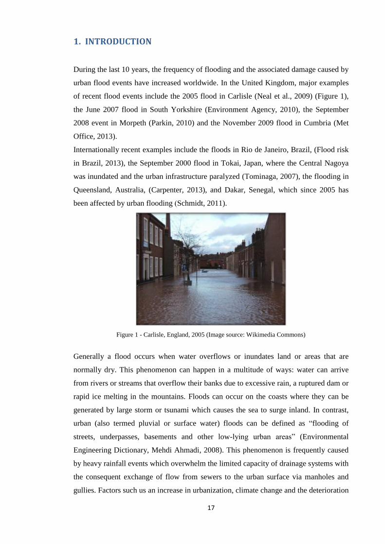
1. INTRODUCTION
During the last 10 years, the frequency of flooding and the associated damage caused by
urban flood events have increased worldwide. In the United Kingdom, major examples
of recent flood events include the 2005 flood in Carlisle (Neal et al., 2009) (Figure 1),
the June 2007 flood in South Yorkshire (Environment Agency, 2010), the September
2008 event in Morpeth (Parkin, 2010) and the November 2009 flood in Cumbria (Met
Office, 2013).
Internationally recent examples include the floods in Rio de Janeiro, Brazil, (Flood risk
in Brazil, 2013), the September 2000 flood in Tokai, Japan, where the Central Nagoya
was inundated and the urban infrastructure paralyzed (Tominaga, 2007), the flooding in
Queensland, Australia, (Carpenter, 2013), and Dakar, Senegal, which since 2005 has
been affected by urban flooding (Schmidt, 2011).
Figure 1 - Carlisle, England, 2005 (Image source: Wikimedia Commons)
Generally a flood occurs when water overflows or inundates land or areas that are
normally dry. This phenomenon can happen in a multitude of ways: water can arrive
from rivers or streams that overflow their banks due to excessive rain, a ruptured dam or
rapid ice melting in the mountains. Floods can occur on the coasts where they can be
generated by large storm or tsunami which causes the sea to surge inland. In contrast,
urban (also termed pluvial or surface water) floods can be defined as “flooding of
streets, underpasses, basements and other low-lying urban areas” (Environmental
Engineering Dictionary, Mehdi Ahmadi, 2008). This phenomenon is frequently caused
by heavy rainfall events which overwhelm the limited capacity of drainage systems with
the consequent exchange of flow from sewers to the urban surface via manholes and
gullies. Factors such us an increase in urbanization, climate change and the deterioration

18
of sewer networks, are expected to contribute to an increase in the number of urban
flood events in the future. For example it is predicted that by 2030, 61% of the world’s
population will be living in urban areas (by that time expected to be approaching 5
billion - Cohen, 2006). In the United Kingdom, the urban population is expected to
increase by 0.73 per cent per year from 2015 until 2020 (World Population Prospect,
2012). The resulting industrial and urban developments cover permeable grounds and
increase the amount of rainwater that runs off the surface into drains and sewers with a
limited capacity. Simultaneously, the effect of climate change (IPCC 2014, Summary
for Policymakers) may increase flood risk as the predicted increased occurrence of
intense rainfall events will place further stress on urban drainage systems (Ashley et al.,
2005).
Finally, many sewerage and drainage networks are operating past their design life. As
these systems deteriorate, there is the potential for urban flood risk to increase due to the
increased occurrence of asset failure such as sewer collapse and blockage, e.g.
Columbo, Sri Lankan capital (WaterWorld, 2012). This particular aspect is not affecting
just the United Kingdom (Defra, 2007) but many other countries and cities around the
world, e.g. Canada (Kerr Wood Leidal Associates LTD, Consulting Engineers, 2008),
San Francisco (City and County of San Francisco, 2030 Sewer System Master Plan),
Delhi (Singh, United Nations University).
It is generally recognized that urban flooding is the most difficult type of flooding to
predict, model and defend against (The Pitt Review, 2008). This is due to the nature of
intense rainfall events (convective, intensive rainfall events which are highly uncertain
and difficult to forecast), the hydraulics of linked sewer and surface flow being complex
and because it is harder to construct cost effective flood defences in urban areas.
Thus, there is a need to provide better modelling capabilities to predict flooding and to
manage flood routes in urban areas. Engineers commonly assess the hydraulic
performance of existing sewer systems using computer models. Whilst these models are
reliable in terms of assessing the below ground system composed of pipes and
manholes, when replicating the phenomenon of flooding into streets they are very
difficult to calibrate and validate due to the paucity of data in real flood conditions. In
particular the uncertainties caused by complex 3D flow fields at the interface between
surface and sub-surface flows are recognized as an important uncertainty within urban
flood models (Djordjević et al., 2005). Current validation datasets in fact often comprise
approximated depth data from CCTV images with poor spatial and temporal resolution.

19
Other desirable datasets such as velocity field and flow exchange are not currently
available. This thesis describes the design and the construction of a new physical model
capable of providing high-resolution experimental datasets in order to calibrate and
validate computational modelling tools. By completing the construction and conducting
initial testing using the physical model, this research provides new understanding of the
hydraulic characteristics of urban flood events.
1.1. Aims of thesis
The aim of this thesis is to develop and test an experimental facility to provide novel
experimental datasets which describe complex sewer and flood flow phenomena such as
above/below ground exchange events.
1.2. Thesis structure
This thesis is organised according to the following structure:
Introduction to the concepts of energy losses and urban flooding, a review of
previous work utilising physical models to describe flows in urban drainage
systems and identification of key research questions to be addressed in this work
(Chapter 2).
A description of the physical models used to answer the research questions
identified, as well as the experimental procedure (Chapter 3).
A presentation and discussion of the results arising from the experimental
program (Chapters 4-5).
A review of the performance of existing hydraulic models when tested against
the experimental data (Chapter 4).
A presentation of the main conclusions of the thesis as well as recommendations
for future work (Chapters 6-7).

20
2 BACKGROUND – LITERATURE REVIEW
The aim of this chapter is to describe the current ‘state of the art’ in terms of urban flood
modelling and the use of physical models as well as defining the knowledge gaps to be
addressed by this thesis.
2.1 Urban flooding
The European Community directive EN 752 defines urban flooding as a “condition
where wastewater and/or surface water escapes from or cannot enter a drain or sewer
system and either remains on the surface or enters buildings” and surcharge as “a
condition in which wastewater and/or surface water is held under pressure within a
gravity drain or sewer system, but does not escape to surface to cause flooding”.
An urban flood is a complex, unsteady hydraulic process, involving interaction between
sewer systems (i.e. pipe network hydraulics) and an urban surface (i.e. free surface
hydraulics, Figure 2). The below ground system (termed the “minor system”) includes
hydraulic structures such as gully systems, manholes as well as pipes which comprise
the conventional urban drainage infrastructure. The above ground system (termed the
“major system”) is made up of different surface flood pathways, which includes roads,
paths, car parks and playing fields.
Figure 2 – Examples of system surcharge and exceedance flow generation. Left) Central Texas,
Herald/TJ MAXWELL, Right) Waynesville, Aug. 9, 2013 Steve Zumwalt/FEMA
The impact of urban flooding (Figure 3) is felt worldwide and it is highly significant as
affected areas are often densely populated and contain vital infrastructure.

21
In addition, due to the flow exchange from the sewer network to the urban surface, land
and property can be flooded with contaminated water (Jha et al, 2011). This is a special
issue for combined sewer systems, which carry foul flow.
Figure 3 – General Urban Flood Events, 1970-2011. Source: EM-DAT: The OFDA/CRED International
Disaster Database www.emdat.be – Universite’ Catholique de Louvain – Brussels, Belgium (Jha et al,
2011).
Each flood can generate different kinds of damage, which may include (Mark. et al.,
2004):
Direct damage, typically material damage caused by water or flowing water;
Indirect damage, such as traffic disruption or production losses;
Social consequences, such as psychological problems for inhabitants as well as
effects on health due to contact with flood water.
ten Veldhuis (2011), created two basic metrics to estimate damage due to flooding.
“Tangible damages”, which include all damages to buildings and infrastructure, and
“intangible damages”, which include damage which is more problematic to calculate,
such as anxiety, trauma and inconvenience.
To achieve a complete quantification of the total damage due to flooding is essential to
incorporate both tangible and intangible damages (Defra, 2004, Ohl and Tapsell, 2000,
Fewtrell and Kay 2008).
To estimate potential damage and quantify risk it is important to understand how water
moves through the urban environment, hence an understanding of the hydraulics of
urban flood flows is critical in order to understand and mitigate risk.
22
2.1.1 Overview of urban flood modelling
Urban flood models utilise the St Venant equations to describe the motion of fluids in
pipes and open channel networks.
Within the minor system the primary direction of flow is defined by the pipe network,
hence a 1D form of the equations can be used. Sewer network hydraulic structures are
commonly represented using empirical minor head loss relationships. Surface flows are
often less constrained, in some floods; flows may follow surface flow paths defined by
street profiles. However, it is also possible that flows may be highly two dimensional at
urban street scales. In which case it is often more desirable to use 2D form of the Saint
Venant equations (at higher computational cost). Models which describe pipe and
surface flows in 1D are termed 1D-1D models. 1D-1D models can provide an adequate
representation of surface flooding as long as flows stay within the street (i.e. 1D
channel) profile (Djordjevic et al., 1999, Mark et al., 2004). Models which describe the
surface flow in 2D are commonly referred to as 1D-2D models. 1D-2D models must
also include coupling of 1D pipe flow models with 2D surface flow models.
The category of 1D-2D models are considered to give the most accurate representation
of urban surface flooding currently available but to achieve this accuracy data and high
computational time are required (Bamford et al., 2008).
Although computational models which describe water flows in pipe and open channels
are generally considered reliable, it is still seen as important to undertake experimental
studies to provide additional results for the calibration and validation of computer
models. Such experimental studies are considered especially valuable when they
provide information of phenomena for which there is a significant lack of calibration
data for modelling results, and the potential accuracy of equations applied is unknown
(Dottori et al., 2013, Notaro et al., 2010, Hunter et al., 2007). Specific examples
relevant to flood modelling include the quantification of head losses within urban
drainage hydraulic structures (such as manholes) with varying geometries, and the
interaction of surface and sewer flows at interaction points such as manholes and
gullies.
Section 2.2 defines the hydraulic principles that need to be considered when analysing
head losses due to manhole structure. Sections 2.3 to 2.5 describe previous experimental
research quantifying losses in manholes and sections 2.6 to 2.9 describe how the

23
interaction of surface and sewer flows is described within current modelling tools and
previous experimental research examining such interactions.
2.2 Conservation of energy and head losses
The total energy of a fluid can be considered to comprise:
Pressure energy;
Kinetic-energy due to velocity;
Gravitational Potential, due to elevation above a given datum.
The energy of a fluid is commonly considered as ‘head’ (with units of length) and
expressed as:
𝑝𝑟𝑒𝑠𝑠𝑢𝑟𝑒 ℎ𝑒𝑎𝑑 = 𝑃
𝜌𝑔 𝑣𝑒𝑙𝑜𝑐𝑖𝑡𝑦 ℎ𝑒𝑎𝑑 =
𝑉2
2𝑔 𝑝𝑜𝑡𝑒𝑛𝑡𝑖𝑎𝑙 ℎ𝑒𝑎𝑑 = 𝑧
Combining these three components it is possible to obtain the total head (H), which is
given by “the Bernoulli equation”:
𝐻 =𝑃
𝜌𝑔+
𝑉
2𝑔
2+ 𝑧 Equation 1
Head loss is the reduction in the total head or pressure (sum of pressure head, velocity
head and elevation head) of a fluid as it moves through a system.
It is impossible to avoid head loss in real fluids. Its presence is due to the friction
between the fluid and the walls of the system where the fluid runs, the friction between
fluid particles as they move relative to another one and the turbulence caused whenever
the flow is redirected or affected in any way, for example as in flow reducers or pumps.
When a liquid is moving from one point to another (1-2) the head losses (hL) can be
expressed as:
ℎ𝐿 = (𝑃1 − 𝑃2
𝜌𝑔) + (
𝑉12− 𝑉2
2
2𝑔) + (𝑧1 − 𝑧2) Equation 2

24
The complex flow pattern in manholes (which includes effect of retardation,
acceleration, rotation in different planes and flow interference) makes it very difficult to
formulate a general theory for energy losses for such structures. One approach to
quantify the energy loss attributed to a manhole is to interpolate the energy grade line
within the pipes on both sides of the manhole (Figure 4). The energy grade lines are
extrapolated to the middle of the manhole and one can then measure the energy loss as
the difference between the lines at the middle of the manhole.
Figure 4 – Pressurized flow with associated energy grade lines and hydraulic grade lines (Asztely, 1995).
Energy loss coefficient (K) for manhole structures are commonly (Marsalek, 1984;
Johnston, 1990; Wang, 1998; Zhao et al., 2006; Ramamurthy, 2007; Mrowiec, 2007;
Phang, 2011; Arao, 2012; Stovin et al., 2013; Pfister, 2014;) defined as:
𝐾 = ∆𝐻2𝑔
𝑉𝑑2 Equation 3
Studies have pointed out the very complex matter of energy losses in manholes. Some
of the parameters which have found to affect the head losses include:
Depth ratio between the upstream branches and the downstream channel (Taylor
1944; Hsu et al., 1998; Gurram & Karki 2000);
Upstream and Downstream hydraulic conditions (i.e. subcritical or supercritical,
Hager 1989, Del Giudice et al., 2000; Del Giudice & Hager 2001, Gargano &
Hager 2002, Gisonni & Hager 2002, Zhao et al., 2004, 2006, 2008);
Effect of bed discordance on the channel junction flow (Biron et al., 1996)
Different flow rates for main pipe and combined lateral pipe (Zhao et al., 2006,
(Ramamurthy & Zhu 1997);

25
Different joining angle between lateral pipe and the main pipe (Pfister &
Gisonni 2014);
Different ratio between water depth in the manhole and pipe diameter
(Ramamurthy & Zhu 1997);
Different ratio between pipe diameter and manhole diameter (Ramamurthy &
Zhu 1997);
Existence of sump inside the manhole and benching effects (Arao et al., 2012);
2.3 Head Losses within In line Manholes
“In line” manholes are commonly defined as manholes with a single inlet and a single
outlet, orientated such that the pipe outlet is directly opposite the pipe inlet. The
hydraulic behaviour and energy losses of “in line” manholes have been investigated by
many researchers.
Studies have been completed investigating behaviour in part-full and pressurized pipes,
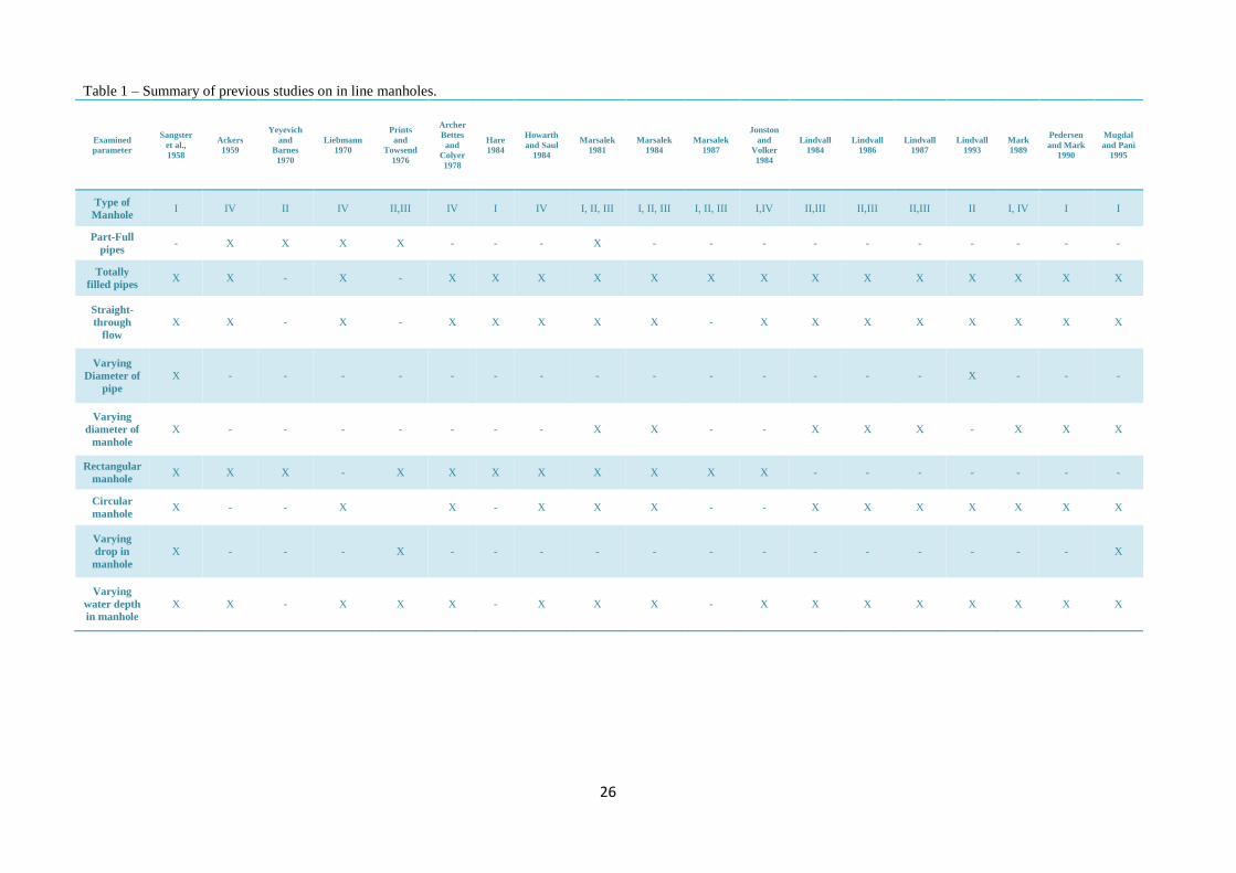
manholes of different sizes and geometries and over a range of hydraulic conditions. A
range of studies and main parameters investigated are summarized in table 1. Manhole
‘types’ are commonly defined based on inflow/outflow pipe configuration, as presented
in figure 5.
Figure 5 – Elevations of typical manholes (surcharged condition) - Asztely (1995).
26
Table 1 – Summary of previous studies on in line manholes.
Examined
parameter
Sangster
et al.,
1958
Ackers
1959
Yeyevich
and
Barnes
1970
Liebmann
1970
Prints
and
Towsend
1976
Archer
Bettes
and
Colyer
1978
Hare
1984
Howarth
and Saul
1984
Marsalek
1981 Marsalek
1984 Marsalek
1987
Jonston
and
Volker
1984
Lindvall
1984 Lindvall
1986 Lindvall
1987 Lindvall
1993 Mark
1989
Pedersen
and Mark
1990
Mugdal
and Pani
1995
Type of
Manhole I IV II IV II,III IV I IV I, II, III I, II, III I, II, III I,IV II,III II,III II,III II I, IV I I
Part-Full
pipes - X X X X - - - X - - - - - - - - - -
Totally
filled pipes X X - X - X X X X X X X X X X X X X X
Straight-
through
flow X X - X - X X X X X - X X X X X X X X
Varying
Diameter of
pipe X - - - - - - - - - - - - - - X - - -
Varying
diameter of
manhole X - - - - - - - X X - - X X X - X X X
Rectangular
manhole X X X - X X X X X X X X - - - - - - -
Circular
manhole X - - X X - X X X - - X X X X X X X
Varying
drop in
manhole X - - - X - - - - - - - - - - - - - X
Varying
water depth
in manhole
X X - X X X - X X X - X X X X X X X X

27
2.3.1 Detail of Selected Previous Studies on In-line Manholes
Sangster et al., (1958) conducted experimental tests on in line manholes (type I) and
pressurized pipes without changes in pipe size and found that the range of energy loss
coefficient K was 0.1-0.2.
Marsalek (1984) reported head loss (K) coefficients observed in a scale model inline
manhole of types I, II and III under both free surface and fully pressurized inflow
conditions with equal inflow and outflow pipes. Energy losses were found to be
approximately proportional to velocity head as predicted by equation 3. K values were
found in the range 0.102 to 0.344 in square shaped manholes, and 0.124 to 0.221 in
circular manholes. K values were found to decrease with decreasing manhole width.
The type of manhole was also found to influence reported K values, with losses for type
I, approximately double that of type III manholes.
Pedersen and Mark (1990) completed experimental tests on in line manholes with fully
submerged inlet and outlet pipes (of equal diameters). Empirical results were used to
define a shape factor (ᶓ) adjustment parameter for different manhole types (table 2),
which quantifies the relative impact of the different geometries on the observed K
values.
Table 2 – Shape factor estimated from measurement with Dm/D up to 4.
Shape Type I Type II Type III
ᶓ 0.24 0.07 0.025
These tests demonstrated the importance of geometry and shape as governing
parameters for the quantification of head losses.
Mrowiec (2007) studied head losses within in line circular type I manholes in drainage
systems under surcharge conditions. The manhole had a 290 mm diameter. Inlet and
outlet pipes were connected to the manhole at the same height and have the same
internal diameter (70 mm). Mrowiec (2007) found that the head loss coefficient for
depths hs/do between 1-3 increases linearly while for Hmh/Dm > 3 had almost a constant
value K=0.45.
Pang and O’Loughlin (2011) measured energy losses within flows passing through a
box-shaped pit (200 mm X 200 mm) without benching, with varying geometric
conditions and flow ranges in both free inflow and submerged conditions. Observed K
values were within the range 0.1-0.4, the authors attempted to relate K values to pit
sizes and pipe diameters, however considerable scatter was observed in trends.
28
Despite numerous studies already completed on energy losses in manholes, due to the
complexity of existing sewer systems, results achieved need to be verified while
considering more variables at the same time (for example benching effects, upstream
and downstream conditions etc.). Computer models rely on these parameters and if local
authorities and governments request the publication of flood hazard maps, which are
very useful for inhabitants, it is crucial to calculate energy loss at manholes including all
variables of structural elements of the pipes and of the manhole which has not been
accomplished yet (Arao et al., 2012).
2.4 Junction Manholes
A “manhole junction” is defined as a manhole which features two or more inflow pipes.
This can cause more complex variations in the flow structures within the manhole;
hence energy losses may be significantly different to those within in line manholes.
Zhao et al., (2006) and Pfister et al., (2014) utilized a common framework for defining
energy loss coefficients at junction manholes, based on the principles of conservation
of mass, energy and momentum.
The local energy losses ∆𝐻𝑖 induced by multiple inlets may be expressed through the
energy equation, can be written as follow (Zhao et al., (2006) and Pfister et al., (2014)):
𝑄1𝐻1 + 𝑄2𝐻2 − 𝑄3𝐻3 = 𝑄3∆𝐻𝑖 Equation 4
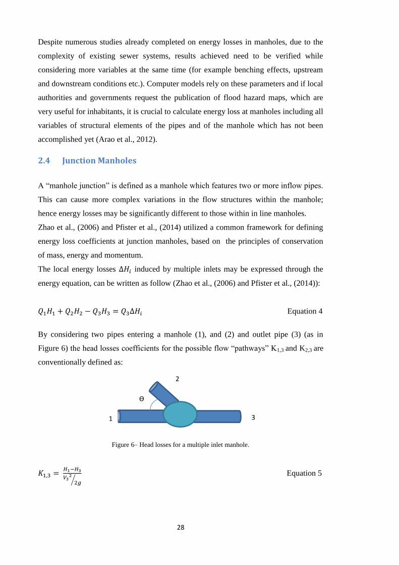
By considering two pipes entering a manhole (1), and (2) and outlet pipe (3) (as in
Figure 6) the head losses coefficients for the possible flow “pathways” K1,3 and K2,3 are
conventionally defined as:
Figure 6– Head losses for a multiple inlet manhole.
𝐾1,3 = 𝐻1−𝐻3
𝑉32
2𝑔⁄
Equation 5
2
=
3 1
Ө
=

29
𝐾2,3 = 𝐻2−𝐻3
𝑉32
2𝑔⁄
Equation 6
The global head loss coefficient for the manhole can be expressed as:
𝐾 = 𝑄1
𝑄3𝐾1,3 +
𝑄2
𝑄3𝐾2,3 Equation 7
A method for determining K values was also produced based on momentum
conservation. Zhao et al., (2006) utilized the conservation of momentum to relate
pressure, flow and inlet orientation, providing the flowing equation:
𝜌(𝑄1𝑉1 + 𝑄2𝑉2 cos 𝜃 − 𝑄3𝑉3) = ∑𝑃𝑥 Equation 8
Where 𝜃 is the junction angle and 𝑃𝑥 are the components of the pressure forces along
the main flow direction. The exchanges of momentum can result in net energy transfer
from the main stream to the merging stream. It is thus possible that due to the changing
plane through which the flow passes, the merging flow may appear leave the junction
manhole with energy content larger than it had upstream. This circumstance implies the
possibility of having an apparent ‘negative’ loss coefficient. However such reported
negative losses (such as in Zhao et al. 2006) are due to the fact that the full system (total
flow in vs total flow out) is not considered and that measurements are taken at a cross-
section where the assumption of straight, parallel streamlines perpendicular to the cross-
section is not met, which is essential for the Bernoulli equation to be valid.
For combining flows, in the case of surcharged manholes, with both inlet pipes and the
outlet pipe pressurized, assuming that the piezometric heads of the approach flows are
equal to the water level in the manhole ( i.e. hydrostatic pressure distribution), Zhao et
al., 2006 defined the terms in equation 9 and 10 to propose a definition for 𝐾 values as
follows:
𝐾1,3 = [1 − 2𝐴3
𝐴1(𝑄1
𝑄3)2− 2
𝐴3
𝐴2(𝑄2
𝑄3)2cos 𝜃 + (
𝐴3
𝐴1)2
(𝑄1
𝑄3)2
] Equation 9
𝐾2,3 = [1 − 2𝐴3
𝐴1(𝑄1
𝑄3)2− 2
𝐴3
𝐴2(𝑄2
𝑄3)2cos𝜃 + (
𝐴3
𝐴2)2
(𝑄2
𝑄3)2
] Equation 10
30
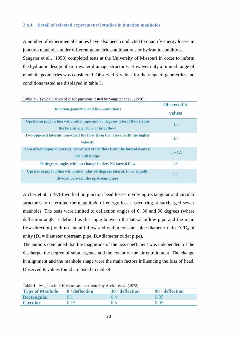
2.4.1 Detail of selected experimental studies in junction manholes
A number of experimental studies have also been conducted to quantify energy losses in
junction manholes under different geometric combinations or hydraulic conditions.
Sangster et al., (1958) completed tests at the University of Missouri in order to inform
the hydraulic design of stormwater drainage structures. However only a limited range of
manhole geometries was considered. Observed K values for the range of geometries and
conditions tested are displayed in table 3.
Table 3 – Typical values of K for junctions tested by Sangster et al., (1958).
Junction geometry and flow conditions Observed K
values
Upstream pipe in line with outlet pipe and 90 degrees lateral flow (from
the lateral one, 20% of total flow) 0.5
Two opposed laterals, one-third the flow from the lateral with the higher
velocity 0.7
Two offset opposed laterals, two-third of the flow from the lateral nearest
the outlet pipe 1.5-1.9
90 degrees angle, without change in size. No lateral flow 1.6
Upstream pipe in line with outlet, plus 90 degrees lateral. Flow equally
divided between the upstream pipes 1.2
Archer et al., (1978) worked on junction head losses involving rectangular and circular
structures to determine the magnitude of energy losses occurring at surcharged sewer
manholes. The tests were limited to deflection angles of 0, 30 and 90 degrees (where
deflection angle is defined as the angle between the lateral inflow pipe and the main
flow direction) with no lateral inflow and with a constant pipe diameter ratio Du/Do of
unity (Du = diameter upstream pipe, Do=diameter outlet pipe).
The authors concluded that the magnitude of the loss coefficient was independent of the
discharge, the degree of submergence and the extent of the air entrainment. The change
in alignment and the manhole shape were the main factors influencing the loss of head.
Observed K values found are listed in table 4:
Table 4 – Magnitude of K values as determined by Archer et al., (1978)
Type of Manhole 0 ᵒ deflection 30 ᵒ deflection 90 ᵒ deflection
Rectangular 0.1 0.4 0.85
Circular 0.15 0.5 0.95

31
Ramamurthy et al., (1997) analyzed combining flows at 90ᵒ junctions within rectangular
closed conduits. Energy loss coefficients were found to vary with the ratio of flows
within the inlet pipes, and the varying size of the size of the lateral inflow pipe.
Observed energy losses coefficients for K12 decreased with increasing of A2/A3 at fixed
Q2/Q3 for rectangular conduits. For high discharge ratios (Q2/Q3 > 0.8) and low values
of area ratios (A2/A1= 0.22) authors found a considerable discrepancy between the
experimental results presented related to K23 for rectangular conduits and existing
results for circular conduits (Serre et al., 1994). This can be explained by the large
difference in the flow structure of combining flows in rectangular conduits and circular
conduits.
Wang et al., (1998) designed an experimental facility (scale 1:6) to determine head
losses at sewer pipe junctions (Manholes) under surcharged conditions. The manholes
studied were type I and tests were conducted for various flow rates, pipe sizes and for
flow configurations including a T-junction, cross and a 90 degrees bend.
Head loss coefficients were in the range K = 0-1.2 and head-loss coefficients were
found to be strongly dependent on the relative inlet flow rate and the change of pipe
diameter within the pipelines, Additionally, head losses become more significant in the
presence of significant lateral inflow or the junction forces a change in flow direction. It
was also found that as the lateral flows become more unequally distributed, the lateral
loss coefficients increase dramatically.
Zhao et al., (2006) and Pfister et al., (2014) compared observed K values within
junction manholes with those predicted by equation 9 and 10. Zhao et al., (2006)
utilized 90° (Figure 7) and 25.8° Edworthy junction (a bespoke junction designed by
Zhao et al., 2006, to replace the problematic T-shaped junction of the Edworthy storm
trunk in the city of Calgary, Alberta, Canada – Figure 8).
The junction chamber was a 3D * 2D rectangular box without benching as shown in
figure 7. The inverts of two inlet pipes connected 5 cm above the bottom of the chamber
and the downstream pipe invert connected 4 cm above.
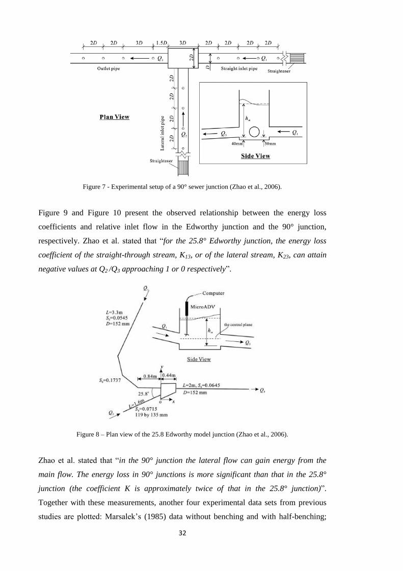
32
Figure 7 - Experimental setup of a 90° sewer junction (Zhao et al., 2006).
Figure 9 and Figure 10 present the observed relationship between the energy loss
coefficients and relative inlet flow in the Edworthy junction and the 90° junction,
respectively. Zhao et al. stated that “for the 25.8° Edworthy junction, the energy loss
coefficient of the straight-through stream, K13, or of the lateral stream, K23, can attain
negative values at Q2 /Q3 approaching 1 or 0 respectively”.
Figure 8 – Plan view of the 25.8 Edworthy model junction (Zhao et al., 2006).
Zhao et al. stated that “in the 90° junction the lateral flow can gain energy from the
main flow. The energy loss in 90° junctions is more significant than that in the 25.8°
junction (the coefficient K is approximately twice of that in the 25.8° junction)”.
Together with these measurements, another four experimental data sets from previous
studies are plotted: Marsalek’s (1985) data without benching and with half-benching;
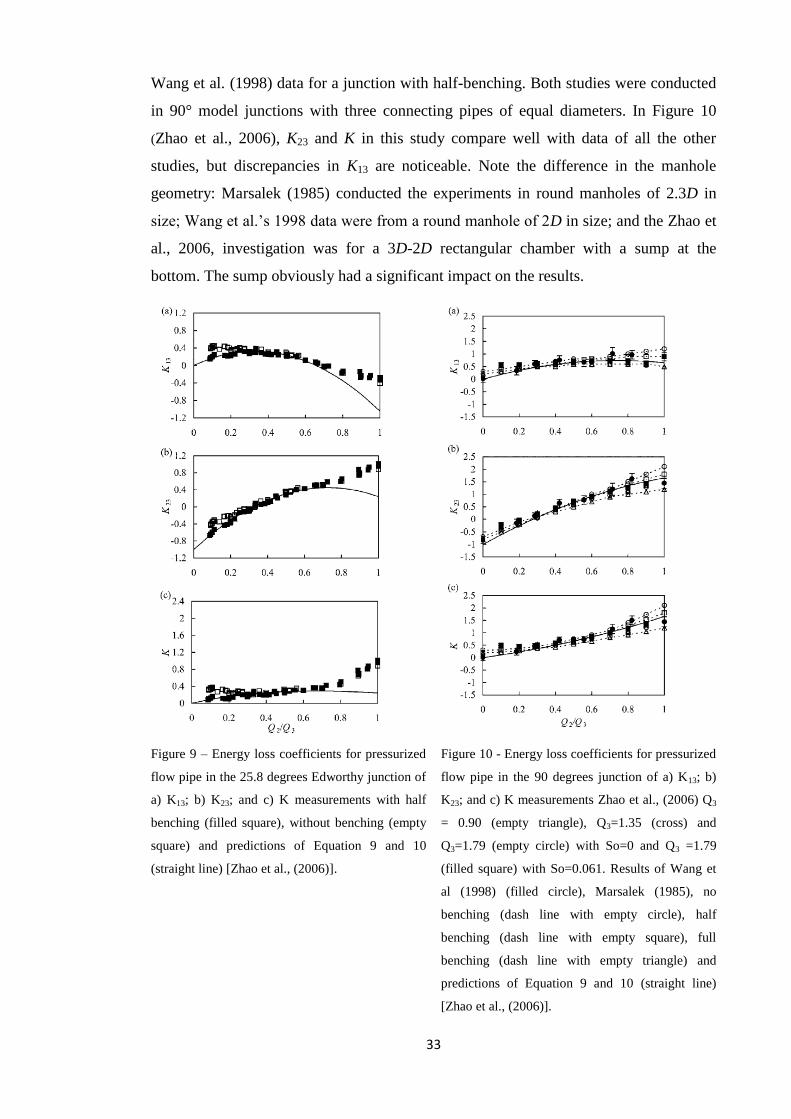
33
Wang et al. (1998) data for a junction with half-benching. Both studies were conducted
in 90° model junctions with three connecting pipes of equal diameters. In Figure 10
(Zhao et al., 2006), K23 and K in this study compare well with data of all the other
studies, but discrepancies in K13 are noticeable. Note the difference in the manhole
geometry: Marsalek (1985) conducted the experiments in round manholes of 2.3D in
size; Wang et al.’s 1998 data were from a round manhole of 2D in size; and the Zhao et
al., 2006, investigation was for a 3D-2D rectangular chamber with a sump at the
bottom. The sump obviously had a significant impact on the results.
Figure 9 – Energy loss coefficients for pressurized
flow pipe in the 25.8 degrees Edworthy junction of
a) K13; b) K23; and c) K measurements with half
benching (filled square), without benching (empty
square) and predictions of Equation 9 and 10
(straight line) [Zhao et al., (2006)].
Figure 10 - Energy loss coefficients for pressurized
flow pipe in the 90 degrees junction of a) K13; b)
K23; and c) K measurements Zhao et al., (2006) Q3
= 0.90 (empty triangle), Q3=1.35 (cross) and
Q3=1.79 (empty circle) with So=0 and Q3 =1.79
(filled square) with So=0.061. Results of Wang et
al (1998) (filled circle), Marsalek (1985), no
benching (dash line with empty circle), half
benching (dash line with empty square), full
benching (dash line with empty triangle) and
predictions of Equation 9 and 10 (straight line)
[Zhao et al., (2006)].

34
Zhao et al. (2006) stated that “it is expected that the sump affects the straight-through
stream more than the lateral one because the discrepancies in the comparisons is
significant in K13 and in K at small Q2 /Q3. The effect of the sump on K vanishes when
the lateral flow become significant. In all of the junctions, good correlations between
the energy loss coefficients and the flow ratio Q2 /Q3 are clear” (results from Zhao et
al., 2006 are plotted in Figure 9 and Figure 10).
Zhao et al. (2006) showed that for the 25.8° Edworthy junction, Equation 9 and 10
describe the variation of the coefficients tolerably well for Q2 /Q3 ratios smaller than
0.7-0.8.
In the 90° junction, Equation 9 and 10 predict K23 well in all junctions tested and the K13
of Zhao et al., (2006) datasets with the exception of tests with a small Q2 /Q3 ratio (as
shown in Figure 10, Zhao et al., 2006). The equation was judge to accurately predict K
at larger Q2/Q3 ratios (when K2 is the largest contributor to overall head loss). However
Equation 9 and 10 omit any effect of benching design in a junction manholes. However,
the authors suggest that the half-benching has little influence on the head loss in the
surcharged flow with the discrepancies at small Q2 /Q3 caused by the sump in the
chamber without benching; in 90° junctions, the effects of the benching in Marsalek
(1985) and Wang et al. (1998) are negligible when inflows are comparable, and only a
fairly small influence on the head loss observed when the lateral flow is dominant.
Therefore, in surcharged flows, common benching designs for sewer junctions with
straight channels and comparable discharges Q1 and Q2 exhibit no significant
contribution to reducing the energy loss. Based on the discussions above, Equation 9
and 10 are expected to provide a good estimate for energy losses for pressurized flow in
90° sewer junctions.
Arao et al., (2012), proposed equations for quantifying energy losses at three-way
circular drop manholes under surcharged conditions which take the influence of the
ratio of the diameter between inflow pipes and outflow pipe and drop gaps between
those pipes into consideration. The outline of the experimental facility developed by
Arao et al. (2012) is illustrated in figure 11.
For this research, Arao et al., (2012) used manhole models with the diameters of 0.15 m
and 0.6 m. As shown in figure 11, the total energy head at inflow and outflow pipes was
calculated at distances of 0.3, 0.5 and 0.7 m from the manhole in terms of equation 1.
The energy loss at a manhole was defined according to equation 3.

35
The increase of energy loss due to the drop gaps (term Su in figure 11) between the main
upstream pipe and the downstream pipe was proposed based on the observed datasets
(equations 11 and 12) and applied for the estimation of energy loss coefficients, K13 and
K23.
𝐶𝑆𝑢 = 1.3 (𝑆𝑢+𝐷𝑢−𝐷𝑑
𝐷𝑢) (
𝐷𝑑
𝐷𝑢)3
(1 −𝑄𝑙
𝑄𝑑)3
𝑖𝑓 0.2 ≤𝑆𝑢+𝐷𝑢−𝐷𝑑
𝐷𝑢 𝑎𝑛𝑑
𝑆𝑢
𝐷𝑑≤ 1.2 Equation 11
𝐶𝑆𝑢 = 1.3 (0.2𝐷𝑑+𝐷𝑢
𝐷𝑢− 0.2) (
𝐷𝑑
𝐷𝑢)3
(1 −𝑄𝑙
𝑄𝑑)3
𝑖𝑓 0.2 ≤𝑆𝑢+𝐷𝑢−𝐷𝑑
𝐷𝑢 𝑎𝑛𝑑
𝑆𝑢
𝐷𝑑> 1.2 Equation 12
Figure 11 – Experimental apparatus (on the right), crown alignment (a), center alignment (b) and
perpendicular connection between inflow and outflow pipes (c) (Arao et al., 2012).
The increase of energy loss due to the drop gaps between the lateral pipe and the
downstream pipe is proposed in equations 13 and 14, which are applied for the
estimation of energy loss coefficient K23.
𝐶𝑆𝑙 = 0.35 (𝑆𝑙+𝐷𝑙−𝐷𝑑
𝐷𝑙) (
𝐷𝑑
𝐷𝑙)3
(𝑄𝑙
𝑄𝑑)3
𝑖𝑓 0 ≤𝑆𝑙+𝐷𝑙−𝐷𝑑
𝐷𝑙 𝑎𝑛𝑑
𝑆𝑙
𝐷𝑑≤ 1 Equation 13
𝐶𝑆𝑙 = 0.35 (𝐷𝑑
𝐷𝑙)3
(𝑄𝑙
𝑄𝑑)3
𝑖𝑓 𝑆𝑙
𝐷𝑑> 1 Equation 14

36
The effect of the drop gaps between the lateral pipe and the downstream pipe was found
to be smaller than the effect of the presence of lateral inflow itself. Arao et al., (2012)
concluded that the energy loss at three-way manhole varies considerably with the ratio
of the diameter between inflow pipes and an outflow pipe, the ratio of flow rate between
those pipes, the water depth in a manhole and the drop gaps between the pipes.
A similar approach has been utilized by Saldarriaga et al., 2012, who constructed a
physical scale model (Figure 12) at the University of Los Andes.
As for other studies measuring hydraulic behaviour, all elements utilized were
constructed of acrylic crystal in order to facilitate the visualization of the hydraulic
conditions inside the structures, in this case pipes and a manhole. Saldarriaga et al.,
2012, investigated supercritical flows inside junction manholes.
Figure 12 – The model of the junction with the correspondent possible variations of the model itself
(Saldarriaga et al., 2012).
The physical model developed by the authors was composed of a main entry pipe and a
lateral of 90° junction angle (Figure 12). Due to the geometry of the system, the study
reproduced three different flow scenarios:
Manhole entry flow through main pipeline only, called direct flow;
Manhole entry flow through lateral pipeline only;
Manhole entry flow through both entry and lateral pipe (junction flow).
To analyze these different flow conditions and obtain governing equations, a statistical
analysis was been completed to develop empirical equations for head loss.
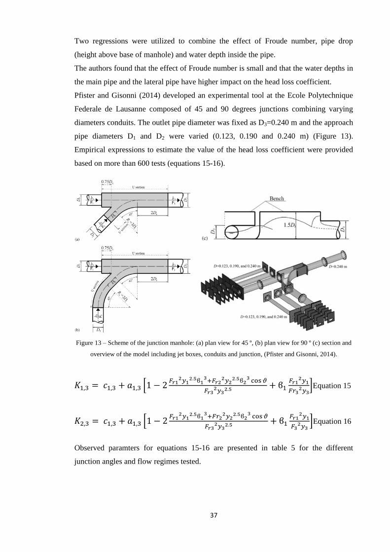
37
Two regressions were utilized to combine the effect of Froude number, pipe drop
(height above base of manhole) and water depth inside the pipe.
The authors found that the effect of Froude number is small and that the water depths in
the main pipe and the lateral pipe have higher impact on the head loss coefficient.
Pfister and Gisonni (2014) developed an experimental tool at the Ecole Polytechnique
Federale de Lausanne composed of 45 and 90 degrees junctions combining varying
diameters conduits. The outlet pipe diameter was fixed as D3=0.240 m and the approach
pipe diameters D1 and D2 were varied (0.123, 0.190 and 0.240 m) (Figure 13).
Empirical expressions to estimate the value of the head loss coefficient were provided
based on more than 600 tests (equations 15-16).
Figure 13 – Scheme of the junction manhole: (a) plan view for 45 º, (b) plan view for 90 º (c) section and
overview of the model including jet boxes, conduits and junction, (Pfister and Gisonni, 2014).
𝐾1,3 = 𝑐1,3 + 𝑎1,3 [1 − 2𝐹𝑟1
2𝑦12.5ϐ1
3+𝐹𝑟22𝑦2
2.5ϐ23 cos𝜗
𝐹𝑟32𝑦3
2.5+ ϐ1
𝐹𝑟12𝑦1
𝐹𝑟32𝑦3]Equation 15
𝐾2,3 = 𝑐1,3 + 𝑎1,3 [1 − 2𝐹𝑟1
2𝑦12.5ϐ1
3+𝐹𝑟22𝑦2
2.5ϐ23 cos𝜗
𝐹𝑟32𝑦3
2.5+ ϐ1
𝐹𝑟12𝑦1
𝐹32𝑦3]Equation 16
Observed paramters for equations 15-16 are presented in table 5 for the different
junction angles and flow regimes tested.

38
Table 5 - Coefficients for equation 15-16 (Pfister et al., 2014)
Junction Angle a 1,3 c 1,3 a 2,3 c 2,3
45ᵒ
Supercritical Flow 0.72 0.27 0.83 0.16
Subcritical Flow 0.91 -0.30 0.75 -0.16
90ᵒ
Supercritical Flow 0.70 0.15 0.68 0.16
Subcritical Flow 0.80 -0.13 0.54 -0.08
2.5 Summary
It can be seen from the reviewed literature that a considerable amount of work has been
conducted to define energy losses through urban drainage hydraulic structures using
physical models. Extensive experimental data are available to estimate local head losses
in free-surface and pressurized flow for “in line” manholes, Flows in angulated
junctions present more complicated patterns, such as waves, mixing, separation,
turbulence, and the transition between (or coexistence of) open channel flow and full
pipe flow and these complex configurations are as important as “in line” manholes.
However for manhole junctions with multiple inlets, existing experimental studies are
largely limited to lateral pipe orientated 90degrees to the inflow and outlet pipes. More
studies would therefore be beneficial using different geometric configurations (for
example 45̊ degrees lateral junctions) and different hydraulic conditions (i.e. under
high/surcharge flow events (Lopes et al., 2013).
2.6 Interaction of below/above ground flows and flow over the
surface
Flood models must also describe the linkages (i.e. flow exchange) between the major
and minor system. An accurate determination of the exchange rates between major and
minor systems is one of the most challenging aspects of urban flood modelling (Mark et
al., 2004). Flood flows through hydraulic structures such as manholes are highly 3D and
unsteady; however within existing models these linkages are most commonly simplified
and expressed using 1D weir and orifice equations, which are obtained by applying the
principles of Bernoulli.
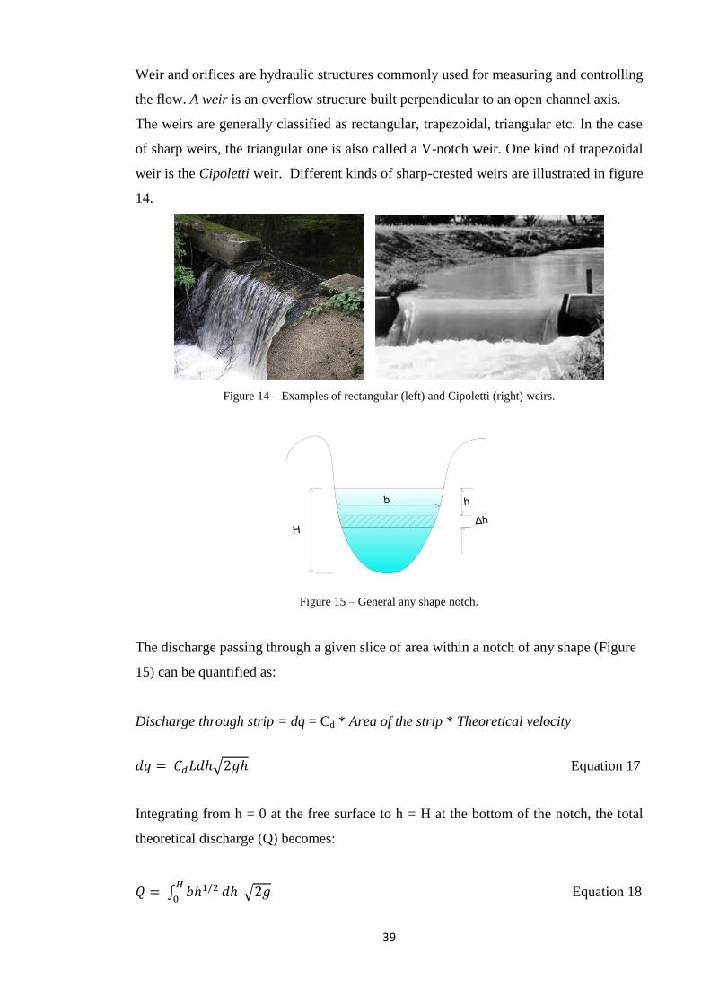
39
Weir and orifices are hydraulic structures commonly used for measuring and controlling
the flow. A weir is an overflow structure built perpendicular to an open channel axis.
The weirs are generally classified as rectangular, trapezoidal, triangular etc. In the case
of sharp weirs, the triangular one is also called a V-notch weir. One kind of trapezoidal
weir is the Cipoletti weir. Different kinds of sharp-crested weirs are illustrated in figure
14.
Figure 14 – Examples of rectangular (left) and Cipoletti (right) weirs.
Figure 15 – General any shape notch.
The discharge passing through a given slice of area within a notch of any shape (Figure
15) can be quantified as:
Discharge through strip = dq = Cd * Area of the strip * Theoretical velocity
𝑑𝑞 = 𝐶𝑑𝐿𝑑ℎ√2𝑔ℎ Equation 17
Integrating from h = 0 at the free surface to h = H at the bottom of the notch, the total
theoretical discharge (Q) becomes:
𝑄 = ∫ 𝑏ℎ1/2 𝑑ℎ √2𝑔𝐻
0 Equation 18
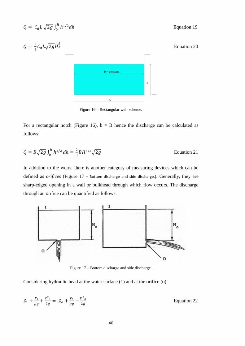
40
𝑄 = 𝐶𝑑𝐿 √2𝑔 ∫ ℎ1/2𝑑ℎ𝐻
0 Equation 19
𝑄 = 2
3𝐶𝑑𝐿√2𝑔𝐻
3
2 Equation 20
Figure 16 – Rectangular weir scheme.
For a rectangular notch (Figure 16), b = B hence the discharge can be calculated as
follows:
𝑄 = 𝐵√2𝑔 ∫ ℎ1/2 𝑑ℎ = 2
3𝐵𝐻3/2√2𝑔
𝐻
0 Equation 21
In addition to the weirs, there is another category of measuring devices which can be
defined as orifices (Figure 17 – Bottom discharge and side discharge.). Generally, they are
sharp-edged opening in a wall or bulkhead through which flow occurs. The discharge
through an orifice can be quantified as follows:
Figure 17 – Bottom discharge and side discharge.
Considering hydraulic head at the water surface (1) and at the orifice (o):
𝑍1 +𝑃1
𝜌𝑔+𝑉21
2𝑔= 𝑍𝑜 +
𝑃0
𝜌𝑔+𝑉20
2𝑔 Equation 22

41
Considering the pressure at (1) and (0) is equal to the atmospheric pressure (P1=P0),
V1=0 and 𝑍1 − 𝑍0 = 𝐻0 gives
𝐻0 = 𝑉20
2𝑔 Equation 23
The velocity of the water passing through the orifice is therefore given by:
𝑉0 = √2𝑔𝐻0 Equation 24
This can be used to quantify the water being discharged through the orifice:
𝑄 = 𝑎𝑉0 = 𝑎√2𝑔𝐻0 Equation 25
In practice the discharge is always less than this theoretical amount due to the viscosity
of the fluid, to surface tension and due to resistance of the air. The disparity between the
theoretical discharge velocity and the actual discharge velocity is accounted for by
introducing a factor Cv known as the Coefficient of Velocity so that:
𝑉𝑎𝑐𝑡𝑢𝑎𝑙 = 𝐶𝑣√2𝑔𝐻0 Equation 26
If the discharge from a sharp edged orifice is examined closely it will be observed that
the minimum diameter of the jet of water discharging from the orifice is smaller than
the orifice diameter. The plane at which this occurs is known as the Vena Contracta,
which is the plane where stream lines first become parallel. Applying the discharge
equation at the vena contracta,
𝑄 = 𝑎𝑐𝐶𝑣√2𝑔𝐻0 Equation 27
This can be written as
𝑄 = 𝑎 𝐶𝑐𝐶𝑣√2𝑔𝐻0 Equation 28
Where 𝐶𝑐 = 𝑎𝑐/𝑎 = Coefficient of Contraction

42
Or more simply as
𝑄 = 𝑎𝐶𝑑√2𝑔𝐻𝑜 Equation 29
Where 𝐶𝑑 = 𝐶𝑐𝐶𝑣 = 𝐶𝑜𝑒𝑓𝑓𝑖𝑐𝑖𝑒𝑛𝑡 𝑜𝑓 𝐷𝑖𝑠𝑐ℎ𝑎𝑟𝑔𝑒 Equation 30
Typical values of Cd range from 0.6 to 0.65 (Massey and Ward-Smith, Mechanics of
Fluids, Seventh Edition, Volume 1). The actual value of the coefficient of discharge for
any orifice may be determined by measuring the quantity of water discharged over a
period of time as well as the head difference upstream and downstream of the orifice.
𝑄 = 𝐶𝑐𝐶𝑣𝑓𝐶𝑣𝑎 𝐴 √2𝑔(ℎ1 − ℎ2) Equation 31
Weir and orifice coefficients depend on the effects of viscosity, the velocity distribution
in the approach section and the capillarity, but they are most commonly determined by
empirical methods (Rouse, 1950).
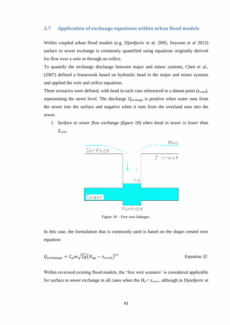
43
2.7 Application of exchange equations within urban flood models
Within coupled urban flood models (e.g. Djordjevic et al. 2005, Seyoum et al 2012)
surface to sewer exchange is commonly quantified using equations originally derived
for flow over a weir or through an orifice.
To quantify the exchange discharge between major and minor systems, Chen et al.,
(2007) defined a framework based on hydraulic head in the major and minor systems
and applied the weir and orifice equations.
Three scenarios were defined, with head in each case referenced to a datum point (zcrest),
representing the street level. The discharge Qexchange is positive when water runs from
the sewer into the surface and negative when it runs from the overland area into the
sewer.
1. Surface to sewer flow exchange (figure 18) when head in sewer is lower than
Zcrest
Figure 18 – Free weir linkages.
In this case, the formulation that is commonly used is based on the shape crested weir
equation:
𝑄𝑒𝑥𝑐ℎ𝑎𝑛𝑔𝑒 = 𝐶𝑤𝑤√2𝑔(𝐻𝑢𝑝 − 𝑧𝑐𝑟𝑒𝑠𝑡)3/2
Equation 32
Within reviewed existing flood models, the ‘free weir scenario’ is considered applicable
for surface to sewer exchange in all cases when the Hd < zcrest , although in Djordjevic et

44
al., (2005), it is noted that a ‘somewhat reduced capacity’ should be considered at high
flow rates when the manhole becomes submerged by the surface flow.
In all reviewed cases, when Hd < zcrest flow in the pipe network is not considered to have
any influence on flow exchange.
This is despite more detailed experimental studies of flows over sharp crested weirs
(e.g. Wu and Rajaratnam, 1996) which have shown the existence of different flow (and
discharge) regimes as a function of flow depth both upstream and downstream of the
weir crest, even when the downstream water level is below the level of the weir crest.
2. Sewer to surface exchange (figure 19) with head above the manhole between
water level on the surface and Zcrest.
Figure 19 – Submerged weir linkage.
In this case:
𝑄𝑒𝑥𝑐ℎ𝑎𝑛𝑔𝑒 = 𝐶𝑤𝑤√2𝑔(𝐻𝑢𝑝 − 𝑧𝑐𝑟𝑒𝑠𝑡)(𝐻𝑢𝑝 − 𝐻𝑑)1/2
Equation 33
This linkage is considered applicable when Hd > Zcrest and Hup < Amh/ᴨDm. If Hup > Amh/
ᴨDm the link is considered ‘fully submerged’ and the submerged orifice formula is
judged a more suitable description of the interface.
The submerged orifice equation can be expressed to provide flow exchange as
𝑄𝑒 = 𝐶𝑖𝐴𝑚ℎ√2𝑔(𝐻𝑢𝑝 − 𝐻𝑑)1
2 Equation 34
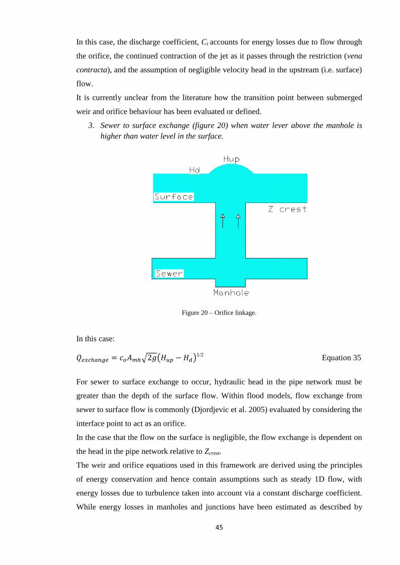
45
In this case, the discharge coefficient, Ci accounts for energy losses due to flow through
the orifice, the continued contraction of the jet as it passes through the restriction (vena
contracta), and the assumption of negligible velocity head in the upstream (i.e. surface)
flow.
It is currently unclear from the literature how the transition point between submerged
weir and orifice behaviour has been evaluated or defined.
3. Sewer to surface exchange (figure 20) when water lever above the manhole is
higher than water level in the surface.
Figure 20 – Orifice linkage.
In this case:
𝑄𝑒𝑥𝑐ℎ𝑎𝑛𝑔𝑒 = 𝑐𝑜𝐴𝑚ℎ√2𝑔(𝐻𝑢𝑝 − 𝐻𝑑)1/2
Equation 35
For sewer to surface exchange to occur, hydraulic head in the pipe network must be
greater than the depth of the surface flow. Within flood models, flow exchange from
sewer to surface flow is commonly (Djordjevic et al. 2005) evaluated by considering the
interface point to act as an orifice.
In the case that the flow on the surface is negligible, the flow exchange is dependent on
the head in the pipe network relative to Zcrest.
The weir and orifice equations used in this framework are derived using the principles
of energy conservation and hence contain assumptions such as steady 1D flow, with
energy losses due to turbulence taken into account via a constant discharge coefficient.
While energy losses in manholes and junctions have been estimated as described by
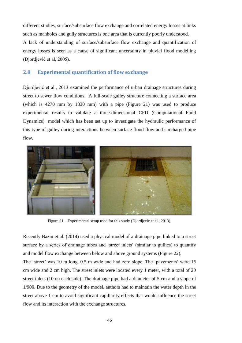
46
different studies, surface/subsurface flow exchange and correlated energy losses at links
such as manholes and gully structures is one area that is currently poorly understood.
A lack of understanding of surface/subsurface flow exchange and quantification of
energy losses is seen as a cause of significant uncertainty in pluvial flood modelling
(Djordjević et al, 2005).
2.8 Experimental quantification of flow exchange
Djordjević et al., 2013 examined the performance of urban drainage structures during
street to sewer flow conditions. A full-scale gulley structure connecting a surface area
(which is 4270 mm by 1830 mm) with a pipe (Figure 21) was used to produce
experimental results to validate a three-dimensional CFD (Computational Fluid
Dynamics) model which has been set up to investigate the hydraulic performance of
this type of gulley during interactions between surface flood flow and surcharged pipe
flow.
Figure 21 – Experimental setup used for this study (Djordjevic et al., 2013).
Recently Bazin et al. (2014) used a physical model of a drainage pipe linked to a street
surface by a series of drainage tubes and ‘street inlets’ (similar to gullies) to quantify
and model flow exchange between below and above ground systems (Figure 22).
The ‘street’ was 10 m long, 0.5 m wide and had zero slope. The ‘pavements’ were 15
cm wide and 2 cm high. The street inlets were located every 1 meter, with a total of 20
street inlets (10 on each side). The drainage pipe had a diameter of 5 cm and a slope of
1/900. Due to the geometry of the model, authors had to maintain the water depth in the
street above 1 cm to avoid significant capillarity effects that would influence the street
flow and its interaction with the exchange structures.
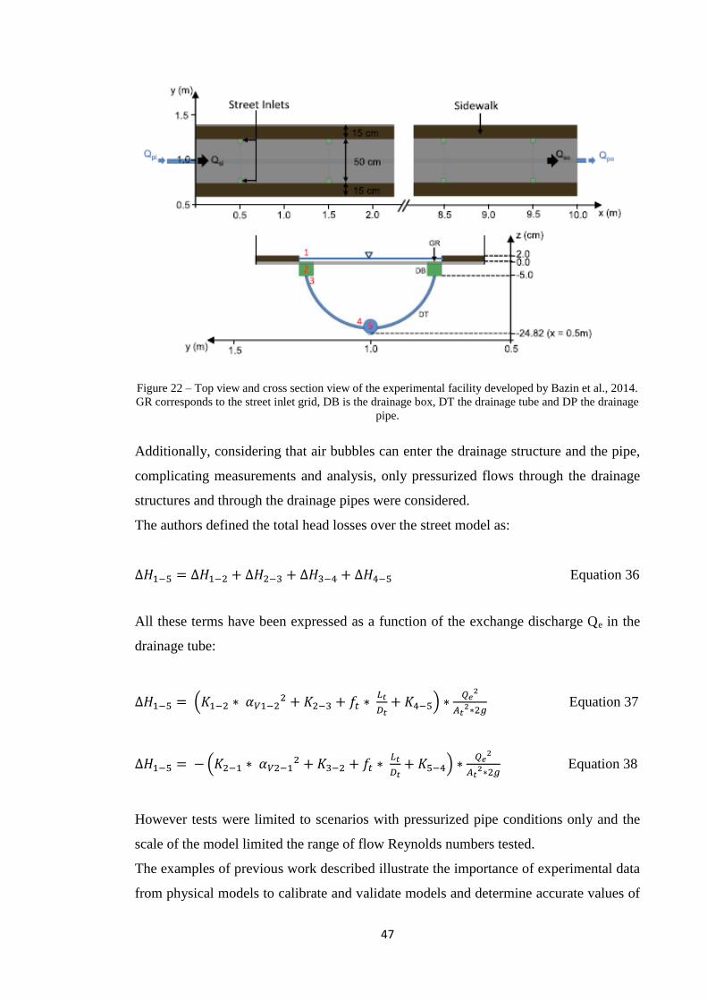
47
Figure 22 – Top view and cross section view of the experimental facility developed by Bazin et al., 2014.
GR corresponds to the street inlet grid, DB is the drainage box, DT the drainage tube and DP the drainage
pipe.
Additionally, considering that air bubbles can enter the drainage structure and the pipe,
complicating measurements and analysis, only pressurized flows through the drainage
structures and through the drainage pipes were considered.
The authors defined the total head losses over the street model as:
∆𝐻1−5 = ∆𝐻1−2 + ∆𝐻2−3 + ∆𝐻3−4 + ∆𝐻4−5 Equation 36
All these terms have been expressed as a function of the exchange discharge Qe in the
drainage tube:
∆𝐻1−5 = (𝐾1−2 ∗ 𝛼𝑉1−22 + 𝐾2−3 + 𝑓𝑡 ∗
𝐿𝑡
𝐷𝑡+ 𝐾4−5) ∗
𝑄𝑒2
𝐴𝑡2∗2𝑔
Equation 37
∆𝐻1−5 = − (𝐾2−1 ∗ 𝛼𝑉2−12 + 𝐾3−2 + 𝑓𝑡 ∗
𝐿𝑡
𝐷𝑡+ 𝐾5−4) ∗
𝑄𝑒2
𝐴𝑡2∗2𝑔
Equation 38
However tests were limited to scenarios with pressurized pipe conditions only and the
scale of the model limited the range of flow Reynolds numbers tested.
The examples of previous work described illustrate the importance of experimental data
from physical models to calibrate and validate models and determine accurate values of

48
Cw and Co. Large uncertainties exist in field datasets due to uncertainties in urban
hydrology and the presence of multiple exchange points.
The suitability of orifice and weir equations and the impacts of assumptions (i.e.
applicability in unsteady flow) on predictive uncertainty have not been explored and
little guidance exists on appropriate discharge coefficients for use within these
equations.
2.9 Existing limitations and gaps in flood modelling tools
Hydraulic flood models rely on parameters to represent flow conditions such as pipe
roughness, energy losses and surcharge. In most cases, during normal operational
conditions in sewer, parameters (such as pipe roughness) can be calibrated with
confidence to the availability of flow data from existing in pipe monitoring.
In contrast, during surcharge and flood events there is a lack of field data suitable for
model calibration and validation (Hunter et al., 2008, Prodanovic et al. 1998). This is
due to two main reasons:
1. High resolution data is expensive and difficult to obtain for long periods of time;
2. Flood events happen relatively infrequently, and thus measurement devices are
highly unlikely to be in the correct place to record data.
Fully instrumented physical models that can reproduce urban flooding events are
therefore very valuable to better understand complex hydraulic processes associated
with urban floods.
Parameters which are highly desirable for the calibration of computer modeling results
but are often difficult to obtain in real scale systems under high or infrequent flow
conditions include:
Energy losses through manhole structures of differing geometries and inlet
conditions.
The flow exchange between minor and major systems during flood events and
energy losses during such interaction events.
Flood wave behavior and velocity fields in shallow urban flood flows.
Existing urban drainage models may use empirical datasets to obtain local head loss
values. However these head loss values may be obtained from observations conducted
in scenarios different to the modelled situation. The variation of head loss values for
typical hydraulic structures such as manholes is currently unclear. In addition the

49
implications for urban drainage models of inaccurate head loss values have not currently
been adequately defined.
Considering the linkage between major and minor system, one significant potential
limitation of flood models concerns the use of weir and orifice equations to represent
exchange rates through manhole structures. Currently there is a significant lack of
calibration data for modelling results, and the potential accuracy of these equations is
unknown, given that they are representing a complex 3D unsteady flow condition using
a constant coefficient to represent energy losses.
2.10 Thesis objectives
The overall aim of this research is to develop a physical urban flood model able to
provide datasets to improve urban pluvial flood models and provide a more accurate
understanding of the hydraulic characteristics of flood flows. By achieving this, the
work will seek to meet the following specific objectives:
1. To verify existing energy head losses for “in line” manholes and providing new
datasets for 45ᵒ manhole junctions, using a physical scale model under a range
of high flow (i.e.surcharged conditions);
2. Evaluate the accuracy of existing computer modelling approaches for describing
flows in urban drainage systems via comparison with a physical model and
quantify the importance of identifying local head losses in computational
models;
3. Assess the suitability of weir and orifice equations for representing the exchange
of flow between major and minor systems during flood flows.
4. Determine appropriate energy loss coefficients for use within weir and orifice
equations when representing flow exchange events.
50
3 METHODOLOGY
This chapter describes the equipment and methodology used to collect and process the
data required to fulfil the aims and objectives described in chapter 2.
This physical modelling can be subdivided into two parts due to the different
configurations that have been developed and used. The first configuration was
constructed to meet research objectives 1 and 2, and comprised a sewer network scale
model featuring six manholes which are connected to each other by five circular pipes
of two different sizes. This configuration was operational from October 2010 to June
2012.
In order to meet research objectives 3 and 4 the second configuration was then
constructed, this comprised a simplified physical model of the sewer network (one
manhole, one pipe) linked to an overhead shallow flow flume, which represented an
urban surface. This configuration was constructed from July 2012 to July 2013 and used
from August 2013 until June 2014.
3.1 Scaling factors and similitudes
When working with a physical experimental model to investigate hydraulic
mechanisms, scaling factors are used to define the geometrical ratio between the real
system and the model. In order that the models faithfully reproduce hydraulic conditions
in the real system, the flows must display a similitude to the real system. In a physical
model, the flow conditions are said to be similar to those in the prototype if the model
displays similarity of form (geometric similarity), similarity of motion (kinematic
similarity) and similarity of forces (dynamic similarity) (Chanson, 1999). Similarity of
these aspects can be determined by a dimensional analysis.
When completing a dimensional analysis for physical models a range of fundamental
parameters need to be considered:
Fluid properties (such as density of water, kg/m3 – dynamic viscosity of water,
Ns/m2);
Channel or flow geometry (characteristics lengths are requested);
Flow properties (such as velocity, m/s).
Considering all these parameters it is possible to complete a dimensional analysis:
𝐹1 (𝜌, µ, , 𝜎, 𝐸𝑏 , 𝑔, 𝐿, 𝑉,𝑃)

51
If mass (M), length (L) and time (T) are chosen as fundamental units, then the
Buckingham -theorem (Buckingham 1915) implies that the quantities can be grouped
into five (5=8-3) independent dimensionless parameters.
𝐹1
(
𝑉
√𝑔𝐿; 𝜌𝑉2
𝑃 ; 𝜌𝑉𝐿
µ ;
𝑉
√𝜎𝜌𝐿
; 𝑉
√𝐸𝑏𝜌 )
𝐹2 (𝐹𝑟 , 𝐸𝑢, 𝑅𝑒 ,𝑊𝑒 ,𝑀𝑎)
Fr number (Froude number) characterizes the ratio of the inertial force to gravity
force;
Eu number (Euler number) shows the proportion of the ration of inertial force to
pressure force;
Re number (Reynolds number) characterizes the ratio of inertial force to viscous
force;
We number (Weber number) is proportional to the ratio of the inertial force to
capillarity force;
Ma number (Sarrau-Mach number) characterizes the ratio of inertial force to
elasticity force.
When reproducing scaled flows in physical models of urban drainage systems two
similitudes are often used: the Reynolds No. (i.e. ratio between inertial/viscous forces)
or the Froude No. (i.e. ratio between inertial/gravitational forces). The similitude
number should be identical in the physical model and at full scale if the hydraulic
phenomena are to be replicated accurately. Reynolds No. is given by:
𝑅𝑒 =𝑉×𝐷ℎ×𝜌
𝜇 Equation 39
Where:
V = average water velocity (m/s)
ρ = water density (= 1000 kg/m3)
μ = dynamic viscosity (= 10-3
kg/sm)
Dh = equivalent diameter (= 4Rh , m)
52
And hence Reynolds similitude is satisfied when:
𝑅𝑒𝑜 = 𝑅𝑒𝑚 Equation 40
Where:
Rem = Reynolds number of the physical model
Reo = Reynolds number of the real system
By applying this similitude the Reynolds Law Ratio of velocity, discharge and time can
be derived as follows:
𝜆𝑅𝑒,𝑣 = 1
𝜆𝑙 Equation 41
𝜆𝑅𝑒,𝑄 = 𝜆𝑣 ∗ 𝜆𝑙2 =
1
𝜆𝑙∗ 𝜆𝑙
2 = 𝜆𝑙 Equation 42
𝜆𝑅𝑒,𝑡 = 𝜆𝑙/𝜆𝑣 = 𝜆𝑙2 Equation 43
If gravitational forces are prevailing (because for example tests are completed in
partially filled pipes), the Froude no. becomes the dominant scale. Froude similitude is
satisfied when:
𝐹𝑟0 = 𝐹𝑟𝑚 = 𝑉𝑜
√𝑔∗𝑦0=
𝑉𝑚
√𝑔∗𝑦𝑚 Equation 44
If λl is the length scale, the corresponding velocity, the volume-flow, time ratios can be
established, using equations 45, 46, 47:
𝜆𝐹𝑟,𝑣 = 𝑉𝑜
𝑉𝑚= √
𝑦𝑜
𝑦𝑚= 𝜆𝑙
12⁄ Equation 45
𝜆𝐹𝑟,𝑄 = 𝜆𝑣 ∗ 𝜆𝑙2 = 𝜆𝑙
52⁄ Equation 46
𝜆𝐹𝑟,𝑡 = 𝜆𝑙/𝜆𝑣 = 𝜆𝑙12⁄ Equation 47

53
3.2 Experimental facility (configuration 1)
Prior to the commencement of the PhD project, a physical model of an urban drainage
was constructed by Darren Unwin (PhD Thesis, 2008 - Development of control
algorithms: to describe flow discharge reduction and energy loss at a manhole
junction). This model was made available for this project.
The model was constructed to represent an equivalent ‘real system’ at 1/6 geometrical
scale. The model consisted of:
Header tank of dimensions 6 m (L) 2.4 m (W) 1.2 m (H);
75 mm (internal) diameter pipework for the main model sections (figure 23a)
(simulating a 450 mm pipe at full scale);
100 mm (internal) diameter pipework for the model outlets (simulating a 600
mm pipe at full scale);
240 mm (internal) diameter pipe utilised as the manhole structures (figure 23b)
(simulating a 1440 mm manhole at full scale).
In addition the laboratory prototype was permanently fitted with the following
instrumentation:
Electro-magnetic (MAG) flow meters (x 3 in the inlet, 2 in the outlet) of 75 mm
internal diameter;
Flow control valves (x 3) of 75 mm internal diameter, butterfly operation fitted
downstream of the flow meters;
Pressure (vertical) sensors, Gems series 5000 (x 21 on the below ground system,
x 6 on the urban surface), 1 on each upstream of the manhole structure, 1 below
each manhole and 1 just downstream from each manhole.
Figure 23 - Examples of scaled pipes on the left (a) and junction manhole on the right (b).
The pipes and manholes were constructed from acrylic due to its ease of workability
(i.e. for when retro-fitting of instrumentation fixtures may be necessary) and its
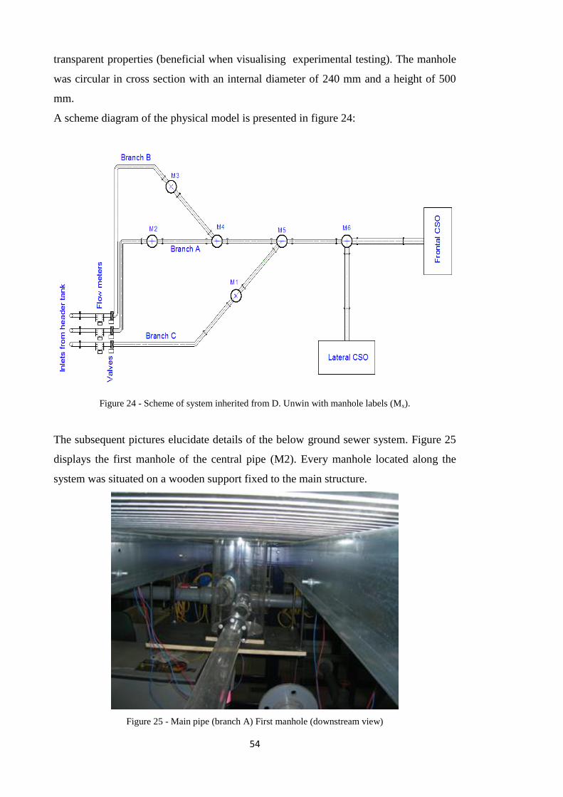
54
transparent properties (beneficial when visualising experimental testing). The manhole
was circular in cross section with an internal diameter of 240 mm and a height of 500
mm.
A scheme diagram of the physical model is presented in figure 24:
Figure 24 - Scheme of system inherited from D. Unwin with manhole labels (Mx).
The subsequent pictures elucidate details of the below ground sewer system. Figure 25
displays the first manhole of the central pipe (M2). Every manhole located along the
system was situated on a wooden support fixed to the main structure.
Figure 25 - Main pipe (branch A) First manhole (downstream view)

55
Figure 26 shows the junction between branch A and the pipe joining from the right with
an angle of 45°, (branch C).
Figure 26 - Main pipe (branch A) Third manhole (downstream view)
Figures 27 display a view of branch C and Figure 28 the overview of the facility.
Figure 27 - Branch “C” (upstream view)
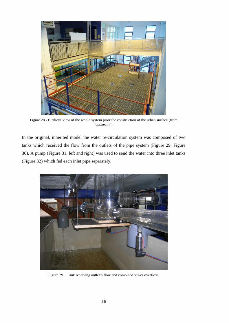
56
Figure 28 - Birdseye view of the whole system prior the construction of the urban surface (from
“upstream”).
In the original, inherited model the water re-circulation system was composed of two
tanks which received the flow from the outlets of the pipe system (Figure 29, Figure
30). A pump (Figure 31, left and right) was used to send the water into three inlet tanks
(Figure 32) which fed each inlet pipe separately.
Figure 29 – Tank receiving outlet’s flow and combined sewer overflow.
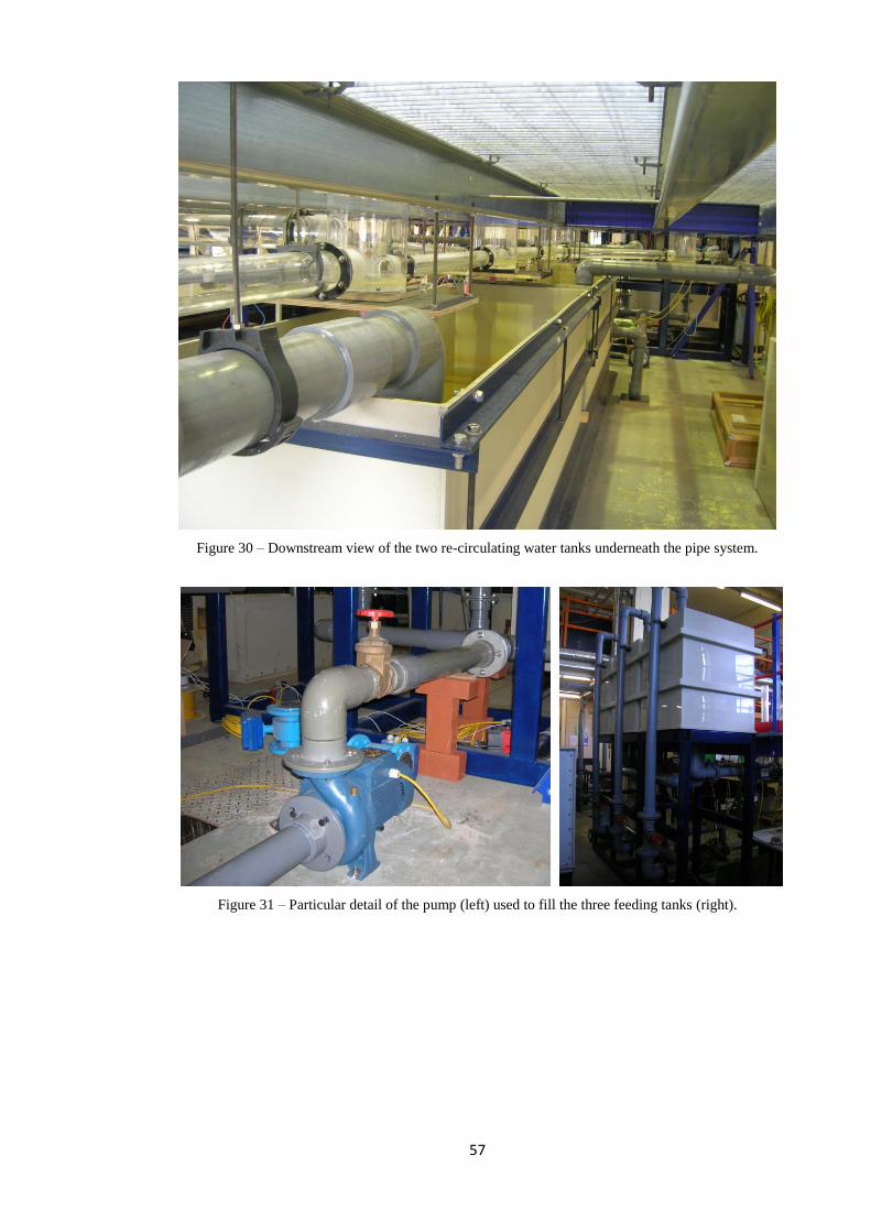
57
Figure 30 – Downstream view of the two re-circulating water tanks underneath the pipe system.
Figure 31 – Particular detail of the pump (left) used to fill the three feeding tanks (right).

58
Figure 32 – Particular detail of the three tanks being filled with water.
On initial testing of the system, it was found that the maximum Reynolds number
achievable was 3*104
(and
only for a short period of time due to the lack of
recirculation), i.e. it was not possible to achieve turbulent conditions inside the pipes. In
order to obtain results scalable to full systems and meet research objectives 1 and 2 it
was therefore necessary to redesign the inlet system such that higher flow rates could be
achieved. Due to practical considerations it was decided that the most straightforward
option to achieve this was to connect the system directly to the main laboratory header
tank (Figure 33 and Figure 34). The tank sits 3.30 m above the physical model hence
can provide a constant head sufficient to achieve much higher flows.
Figure 33 – Full view of the new inlet system.
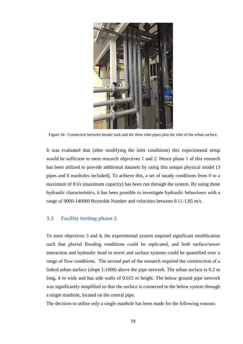
59
Figure 34– Connection between header tank and the three inlet pipes plus the inlet of the urban surface.
It was evaluated that (after modifying the inlet conditions) this experimental setup
would be sufficient to meet research objectives 1 and 2. Hence phase 1 of this research
has been utilized to provide additional datasets by using this unique physical model (3
pipes and 6 manholes included). To achieve this, a set of steady conditions from 0 to a
maximum of 8 l/s (maximum capacity) has been run through the system. By using these
hydraulic characteristics, it has been possible to investigate hydraulic behaviours with a
range of 9000-140000 Reynolds Number and velocities between 0.11-1.85 m/s.
3.3 Facility testing phase 2
To meet objectives 3 and 4, the experimental system required significant modification
such that pluvial flooding conditions could be replicated, and both surface/sewer
interaction and hydraulic head in sewer and surface systems could be quantified over a
range of flow conditions. The second part of the research required the construction of a
linked urban surface (slope 1:1000) above the pipe network. The urban surface is 8.2 m
long, 4 m wide and has side walls of 0.015 m height. The below ground pipe network
was significantly simplified so that the surface is connected to the below system through
a single manhole, located on the central pipe.
The decision to utilise only a single manhole has been made for the following reasons:
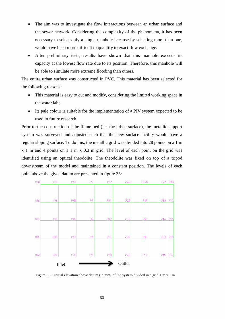
60
The aim was to investigate the flow interactions between an urban surface and
the sewer network. Considering the complexity of the phenomena, it has been
necessary to select only a single manhole because by selecting more than one,
would have been more difficult to quantify to exact flow exchange.
After preliminary tests, results have shown that this manhole exceeds its
capacity at the lowest flow rate due to its position. Therefore, this manhole will
be able to simulate more extreme flooding than others.
The entire urban surface was constructed in PVC. This material has been selected for
the following reasons:
This material is easy to cut and modify, considering the limited working space in
the water lab;
Its pale colour is suitable for the implementation of a PIV system expected to be
used in future research.
Prior to the construction of the flume bed (i.e. the urban surface), the metallic support
system was surveyed and adjusted such that the new surface facility would have a
regular sloping surface. To do this, the metallic grid was divided into 28 points on a 1 m
x 1 m and 4 points on a 1 m x 0.3 m grid. The level of each point on the grid was
identified using an optical theodolite. The theodolite was fixed on top of a tripod
downstream of the model and maintained in a constant position. The levels of each
point above the given datum are presented in figure 35:
Figure 35 – Initial elevation above datum (in mm) of the system divided in a grid 1 m x 1 m
Inlet Outlet

61
The maximum range between inlet and outlet was originally 37 mm, with considerable
variation in the lateral dimension. To rectify the grid system in order to obtain the
correct slope for the overlaying flume bed, thin metallic washers were added to the
metallic structure in appropriate points. After modification and further verification, a
shallow flow flume was constructed over the top of the metallic grid, with additional
pressure transducers located around the manhole (Figure 37 and Figure 38).
Figure 36 – Plan view of the urban surface.
Figure 37 –Location of the pressure measurement points (distances in mm) on the urban surface around
the manhole.

62
Figure 38 –Plan view of the pressure measurement points (Px) on the urban surface around the manhole.
Inlet and outlet tanks were constructed upstream and downstream of the urban surface
model (Figure 36).
The inlet tank (dimensions L= 4 m, W= 0.3 m, H= 0.35 m) receives water from a 75
mm pipe connected to the main laboratory header tank.
Inflow rates are controlled by an in line valve (on the inflow pipe) which can be
regulated both manually and by the command of LabVIEW software (section 3.4). In
addition, the pipe is fitted with a mag flow meter connected to LABVIEW (section 3.4)
such that inflow rates can be monitored in real time.
Inflow and outflow weirs were also constructed to ensure a regular inflow and outflow
over the entire width of the model. The downstream (outlet) weir is manually adjustable
to allow a greater degree of control of flow depth on the model urban surface. The inlet
tank has been filled with baffle material so that flow disturbances around the inflow
pipe do not caused uneven flow over the inflow weir (Figure 39). The inlet tank also
contains a 75 mm internal diameter drain for emergency in case of a failure of the
system (e.g. electrical blackout during the simulation, inability to close the valves with
LabVIEW software).
D=240 mm
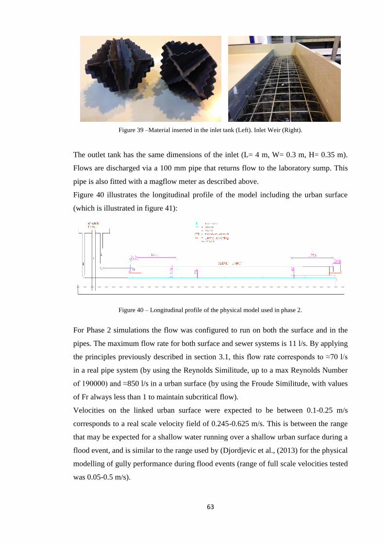
63
Figure 39 –Material inserted in the inlet tank (Left). Inlet Weir (Right).
The outlet tank has the same dimensions of the inlet (L= 4 m, W= 0.3 m, H= 0.35 m).
Flows are discharged via a 100 mm pipe that returns flow to the laboratory sump. This
pipe is also fitted with a magflow meter as described above.
Figure 40 illustrates the longitudinal profile of the model including the urban surface
(which is illustrated in figure 41):
Figure 40 – Longitudinal profile of the physical model used in phase 2.
For Phase 2 simulations the flow was configured to run on both the surface and in the
pipes. The maximum flow rate for both surface and sewer systems is 11 l/s. By applying
the principles previously described in section 3.1, this flow rate corresponds to ≈70 l/s
in a real pipe system (by using the Reynolds Similitude, up to a max Reynolds Number
of 190000) and ≈850 l/s in a urban surface (by using the Froude Similitude, with values
of Fr always less than 1 to maintain subcritical flow).
Velocities on the linked urban surface were expected to be between 0.1-0.25 m/s
corresponds to a real scale velocity field of 0.245-0.625 m/s. This is between the range
that may be expected for a shallow water running over a shallow urban surface during a
flood event, and is similar to the range used by (Djordjevic et al., (2013) for the physical
modelling of gully performance during flood events (range of full scale velocities tested
was 0.05-0.5 m/s).

64
Figure 41- Urban surface: on the left view from the upstream, on the right view from the downstream.

65
3.4 Managing and controlling the model (testing phase 1 and 2)
The physical model is instrumented to provide the following outputs which are directly
collected by a LabVIEW interface:
- flow at each inlet to the model;
- flow at each outlet;
- water depth in the pipes at 27 locations;
- water level in each manhole;
- valves opening ratio.
LabVIEW software is used to control the valve openings and to acquire data in real
time.
Figure 42 – Instrumentation scheme on the pipe network (phase 1 setup).
LabVIEW works through a double file: one called “Front Panel” where the controllers
and indicators of the system can be checked and another one called “Block Diagram”
where there is a scheme of the system that must be measured and controlled. This
instrumentation can control the range of values in multiple formats (Ampere, Volts, and
I/O Boolean). This is a fundamental step because all the output signals from the PAC
(Programmable Automation Controllers) hardware are electrical (Boolean, current or
voltage) and they must be converted into physical parameters such as water depth.
All the electrical outputs from the instrumentation can be checked through an IP address
assigned to each series of data. The internet connection was also used to send input

66
signals to the hardware and subsequently to the model. In this way, simulations can also
be conducted if the operator is not physically present by using internet connection to
activate and deactivate all the system control and instrumentation devices.
The VI shown in figure 43 has been used to manage the rig tests. This software enables
a good visualization of the data in real time, permitting visualization of the flow through
the pipes as well as water depth in the manholes.

67
Figure 43– Front panel of the interface developed.
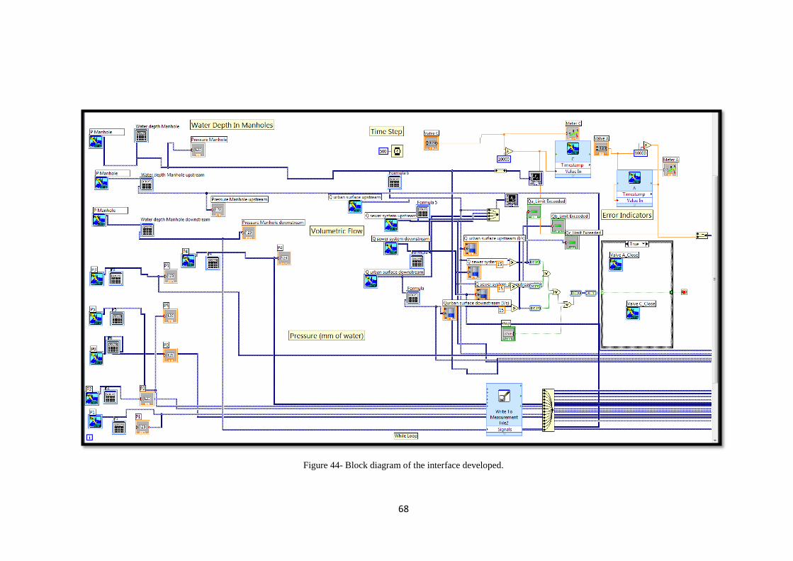
68
Figure 44- Block diagram of the interface developed.
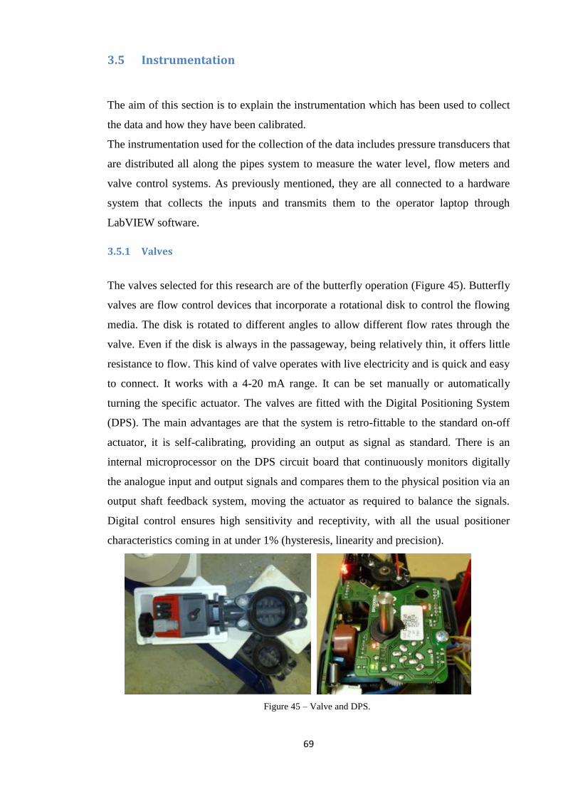
69
3.5 Instrumentation
The aim of this section is to explain the instrumentation which has been used to collect
the data and how they have been calibrated.
The instrumentation used for the collection of the data includes pressure transducers that
are distributed all along the pipes system to measure the water level, flow meters and
valve control systems. As previously mentioned, they are all connected to a hardware
system that collects the inputs and transmits them to the operator laptop through
LabVIEW software.
3.5.1 Valves
The valves selected for this research are of the butterfly operation (Figure 45). Butterfly
valves are flow control devices that incorporate a rotational disk to control the flowing
media. The disk is rotated to different angles to allow different flow rates through the
valve. Even if the disk is always in the passageway, being relatively thin, it offers little
resistance to flow. This kind of valve operates with live electricity and is quick and easy
to connect. It works with a 4-20 mA range. It can be set manually or automatically
turning the specific actuator. The valves are fitted with the Digital Positioning System
(DPS). The main advantages are that the system is retro-fittable to the standard on-off
actuator, it is self-calibrating, providing an output as signal as standard. There is an
internal microprocessor on the DPS circuit board that continuously monitors digitally
the analogue input and output signals and compares them to the physical position via an
output shaft feedback system, moving the actuator as required to balance the signals.
Digital control ensures high sensitivity and receptivity, with all the usual positioner
characteristics coming in at under 1% (hysteresis, linearity and precision).
Figure 45 – Valve and DPS.
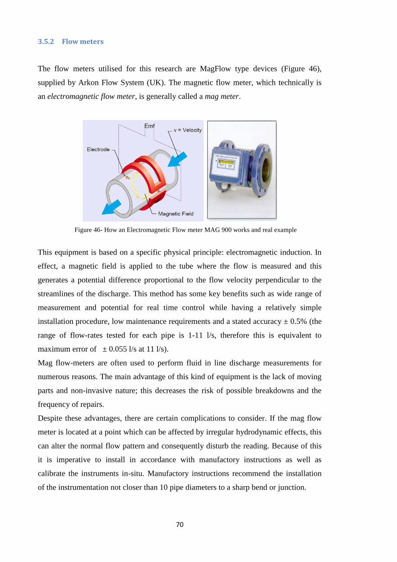
70
3.5.2 Flow meters
The flow meters utilised for this research are MagFlow type devices (Figure 46),
supplied by Arkon Flow System (UK). The magnetic flow meter, which technically is
an electromagnetic flow meter, is generally called a mag meter.
Figure 46- How an Electromagnetic Flow meter MAG 900 works and real example
This equipment is based on a specific physical principle: electromagnetic induction. In
effect, a magnetic field is applied to the tube where the flow is measured and this
generates a potential difference proportional to the flow velocity perpendicular to the
streamlines of the discharge. This method has some key benefits such as wide range of
measurement and potential for real time control while having a relatively simple
installation procedure, low maintenance requirements and a stated accuracy ± 0.5% (the
range of flow-rates tested for each pipe is 1-11 l/s, therefore this is equivalent to
maximum error of ± 0.055 l/s at 11 l/s).
Mag flow-meters are often used to perform fluid in line discharge measurements for
numerous reasons. The main advantage of this kind of equipment is the lack of moving
parts and non-invasive nature; this decreases the risk of possible breakdowns and the
frequency of repairs.
Despite these advantages, there are certain complications to consider. If the mag flow
meter is located at a point which can be affected by irregular hydrodynamic effects, this
can alter the normal flow pattern and consequently disturb the reading. Because of this
it is imperative to install in accordance with manufactory instructions as well as
calibrate the instruments in-situ. Manufactory instructions recommend the installation
of the instrumentation not closer than 10 pipe diameters to a sharp bend or junction.

71
The flow-meters utilised in this research were 75mm internal diameter. Considering the
limitation in terms of space available in the water laboratory, to design the downstream
section for the re-circulation of the water a “T” connection has been necessarily utilized
for the two downstream flow meters (Figure 47 – Figure 48).
Figure 47 - Suggested location for Mag Flow Meters (MAG Flow Meter, Installation Manual,
Ver.2001-1).
Figure 48 - “T” connection utilized for pipe downstream urban surface as well as sewer system.
3.5.3 Pressure transducers
The pressure transducers utilized for this research are the “Series 5000 GEMS sensors”
(Figure 49). This kind of transducer converts fluid pressures into a proportional
electrical signal.

72
Figure 49 – Pressure transducers GEMS
These pressure transducers require a specific periodic inspection of the cable and
moulding because it is important to constantly guarantee that they do not suffer damage.
Every day before each test, the pressure transducers were checked and cleaned with a
small amount of water introduced gently with a syringe to avoid the deposit of any
material from the previous tests which may cause erroneous results.
3.6 Calibration of Instrumentation
3.6.1 Pressure sensor calibration
Each pressure sensor and valve has been calibrated to determine the relationship
between pressure and electrical output signal for each pressure sensor. The specified
pressure range of the sensors is 0-70mb, and the specified electrical output ranges
between 4-20mA. During calibration pressure is determined by measurement of water
depth above the pressure sensor. For the pressure sensors used in phase 1, the
calibration has been carried out within the pipe network facility using the following
methodology (Figure 50):
Set the valve opening and record in a spreadsheet the signal sent by the pressure
sensor after a stabilization of 300 seconds for each valve opening.
Record the water depth in the manhole for each valve opening after the
stabilization.
Plot the correlation between the sensor output Amperes and the measured water
depth of the manhole (directly related to pressure).
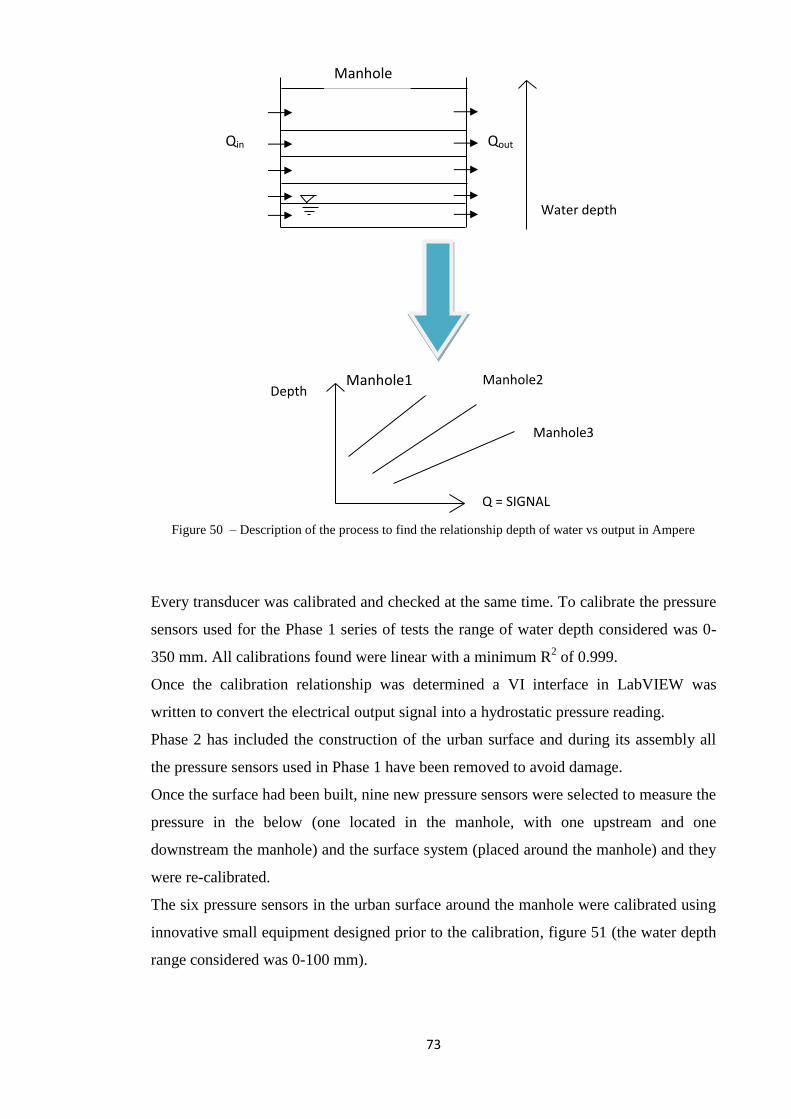
73
Figure 50 – Description of the process to find the relationship depth of water vs output in Ampere
Every transducer was calibrated and checked at the same time. To calibrate the pressure
sensors used for the Phase 1 series of tests the range of water depth considered was 0-
350 mm. All calibrations found were linear with a minimum R2 of 0.999.
Once the calibration relationship was determined a VI interface in LabVIEW was
written to convert the electrical output signal into a hydrostatic pressure reading.
Phase 2 has included the construction of the urban surface and during its assembly all
the pressure sensors used in Phase 1 have been removed to avoid damage.
Once the surface had been built, nine new pressure sensors were selected to measure the
pressure in the below (one located in the manhole, with one upstream and one
downstream the manhole) and the surface system (placed around the manhole) and they
were re-calibrated.
The six pressure sensors in the urban surface around the manhole were calibrated using
innovative small equipment designed prior to the calibration, figure 51 (the water depth
range considered was 0-100 mm).
Q = SIGNAL
Depth
Manhole3
Manhole1 Manhole2
Manhole
Qin Qout
Water depth
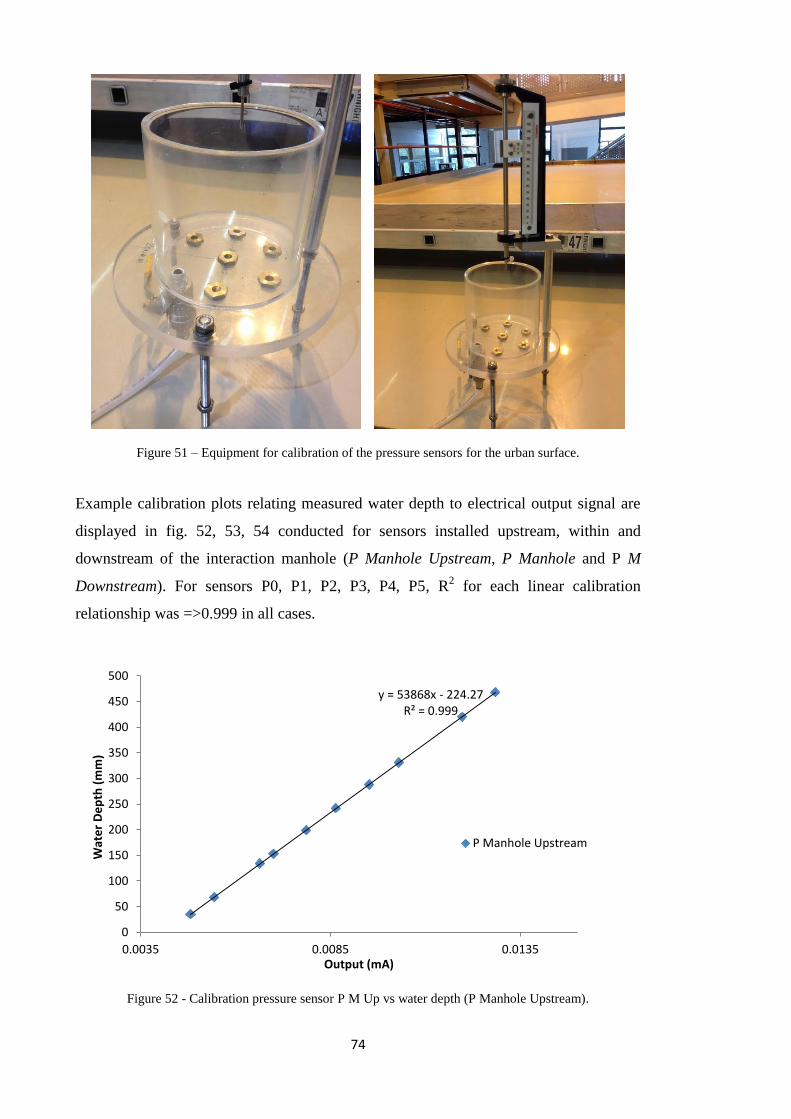
74
Figure 51 – Equipment for calibration of the pressure sensors for the urban surface.
Example calibration plots relating measured water depth to electrical output signal are
displayed in fig. 52, 53, 54 conducted for sensors installed upstream, within and
downstream of the interaction manhole (P Manhole Upstream, P Manhole and P M
Downstream). For sensors P0, P1, P2, P3, P4, P5, R2 for each linear calibration
relationship was =>0.999 in all cases.
Figure 52 - Calibration pressure sensor P M Up vs water depth (P Manhole Upstream).
y = 53868x - 224.27 R² = 0.999
0
50
100
150
200
250
300
350
400
450
500
0.0035 0.0085 0.0135
Wat
er
De
pth
(m
m)
Output (mA)
P Manhole Upstream
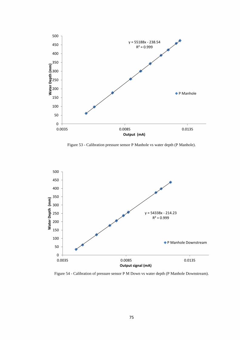
75
Figure 53 - Calibration pressure sensor P Manhole vs water depth (P Manhole).
Figure 54 - Calibration of pressure sensor P M Down vs water depth (P Manhole Downstream).
y = 55188x - 238.54 R² = 0.999
0
50
100
150
200
250
300
350
400
450
500
0.0035 0.0085 0.0135
Wat
er
De
pth
(m
m)
Output (mA)
P Manhole
y = 54338x - 214.23 R² = 0.999
0
50
100
150
200
250
300
350
400
450
500
0.0035 0.0085 0.0135
Wat
er
De
pth
(m
m)
Output signal (mA)
P Manhole Downstream

76
3.6.2 Valve calibration
The purpose of the valve calibration is to determine the relationship between the valve
input (mA) set by the operator (which directly controls the valve opening) and the flow
rate (l/s) into the system as recorded by the flow meters.
Once this relationship is determined, it is possible to control the flow rate independently
via the LABVIEW system and to stipulate time varying flow rates by assigning an
opening ratio vs time relationship to the valves using a simple VI in LabVIEW. The
methodology for calibration is:
1. Set the valve opening until a flow in the pipe is detected
2. Let the flow stabilize for 5 minutes
3. For the following 5 minutes read the flow rate (m3/hr) from the flow-meter every
5 seconds and record at the same time the input and output signal of the flow
meter (Amps) in a spreadsheet file.
4. Then increase the valve opening signal by 0.1 mA and repeat steps 2 and 3.
5. At the end of the simulation time average the recorded data to obtain a unique
value of flow rate (l/s) and input and output signals (Amps) for each valve
opening.
6. Plot the correlation between the valve opening (mA) and average flow rate
recorded (l/s) and also between the average output signal from the flow meter
(Amperes) and average flow rate recorded (l/s).
Figure 55 – Process for the calibration of the flow with the opening and the closure of the valves and the
final interpolation of the data.
Flow meter
output signal (A) Time Valve opening (A)
Opening
Closure
F
l
o
w
r
a
t
e
F
l
o
w
r
a
t
e
F
l
o
w
r
a
t
e
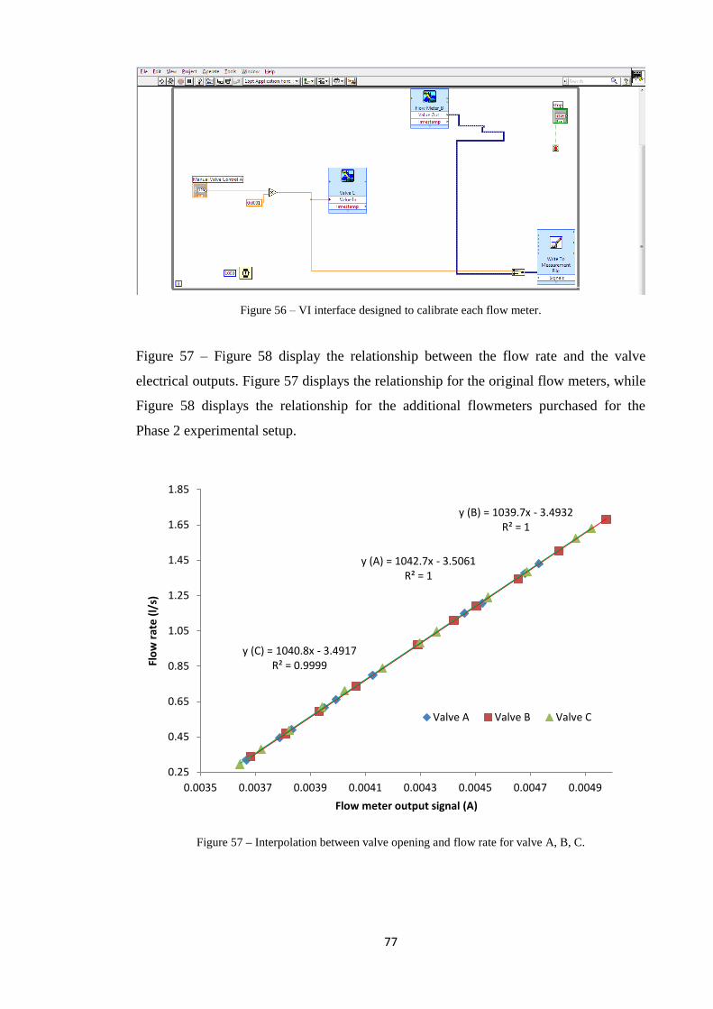
77
Figure 56 – VI interface designed to calibrate each flow meter.
Figure 57 – Figure 58 display the relationship between the flow rate and the valve
electrical outputs. Figure 57 displays the relationship for the original flow meters, while
Figure 58 displays the relationship for the additional flowmeters purchased for the
Phase 2 experimental setup.
Figure 57 – Interpolation between valve opening and flow rate for valve A, B, C.
y (A) = 1042.7x - 3.5061 R² = 1
y (B) = 1039.7x - 3.4932 R² = 1
y (C) = 1040.8x - 3.4917 R² = 0.9999
0.25
0.45
0.65
0.85
1.05
1.25
1.45
1.65
1.85
0.0035 0.0037 0.0039 0.0041 0.0043 0.0045 0.0047 0.0049
Flo
w r
ate
(l/
s)
Flow meter output signal (A)
Valve A Valve B Valve C
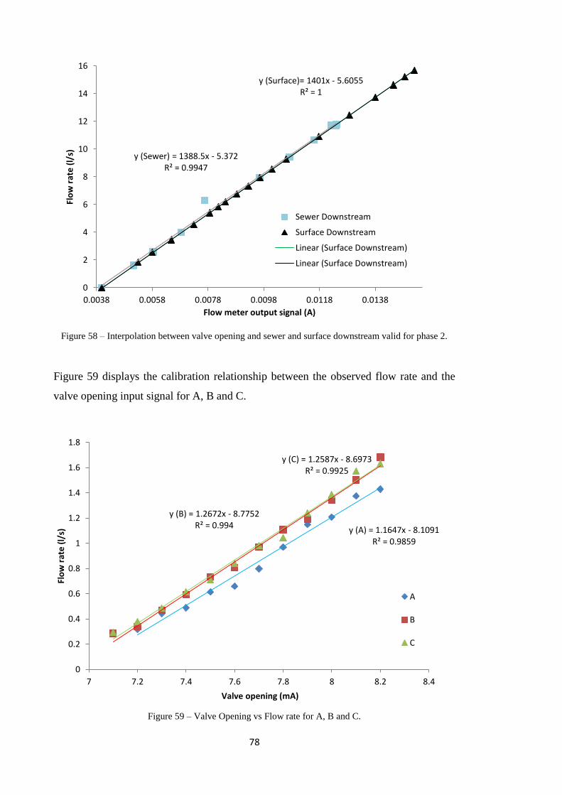
78
Figure 58 – Interpolation between valve opening and sewer and surface downstream valid for phase 2.
Figure 59 displays the calibration relationship between the observed flow rate and the
valve opening input signal for A, B and C.
Figure 59 – Valve Opening vs Flow rate for A, B and C.
y (Sewer) = 1388.5x - 5.372 R² = 0.9947
y (Surface)= 1401x - 5.6055 R² = 1
0
2
4
6
8
10
12
14
16
0.0038 0.0058 0.0078 0.0098 0.0118 0.0138
Flo
w r
ate
(l/
s)
Flow meter output signal (A)
Sewer Downstream
Surface Downstream
Linear (Surface Downstream)
Linear (Surface Downstream)
y (A) = 1.1647x - 8.1091 R² = 0.9859
y (B) = 1.2672x - 8.7752 R² = 0.994
y (C) = 1.2587x - 8.6973 R² = 0.9925
0
0.2
0.4
0.6
0.8
1
1.2
1.4
1.6
1.8
7 7.2 7.4 7.6 7.8 8 8.2 8.4
Flo
w r
ate
(l/
s)
Valve opening (mA)
A
B
C

79
Once the calibration of the input electrical signals was complete, a verification set of
tests have been conducted to compare the flow rate measured by the values against the
values provided by the laboratory measurement tank.
These confirmation tests were only conducted during the phase two tests. Two tests
were conducted; one using the ‘sewer’ inflow and outflow meters, and one using the
‘surface’ inflow and outflow meters (Figure 60 – Figure 61).
Figure 60 – Calibration tests sewer flow meters vs measurement tank prior to correction factor
Figure 61 - Calibration tests surface flow meters prior to correction factor.
0.00
2.00
4.00
6.00
8.00
10.00
12.00
2.00 3.00 4.00 5.00 6.00 7.00 8.00 9.00 10.00 11.00 12.00
Flo
w in
, ou
t se
we
r sy
ste
m r
eco
rde
d (
l/s)
Flow measurement tank (l/s)
Flow recorded with the inletsewer flowmeter
Flow recorded with the outletsewer flowmeter
Flow calculated with themeasuring tank
0.00
2.00
4.00
6.00
8.00
10.00
12.00
14.00
0.00 2.00 4.00 6.00 8.00 10.00 12.00
Flo
w in
, ou
t u
rban
su
rfac
e r
eco
rde
d (
l/s)
Flow measurement tank (l/s)
Flow recorded with the inletsurface flowmeter
Flow recorded with the outletsurface flowmeter
Flow calculated with themeasuring tank
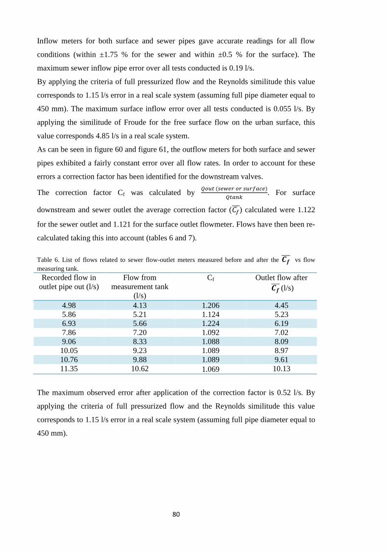
80
Inflow meters for both surface and sewer pipes gave accurate readings for all flow
conditions (within ±1.75 % for the sewer and within ±0.5 % for the surface). The
maximum sewer inflow pipe error over all tests conducted is 0.19 l/s.
By applying the criteria of full pressurized flow and the Reynolds similitude this value
corresponds to 1.15 l/s error in a real scale system (assuming full pipe diameter equal to
450 mm). The maximum surface inflow error over all tests conducted is 0.055 l/s. By
applying the similitude of Froude for the free surface flow on the urban surface, this
value corresponds 4.85 l/s in a real scale system.
As can be seen in figure 60 and figure 61, the outflow meters for both surface and sewer
pipes exhibited a fairly constant error over all flow rates. In order to account for these
errors a correction factor has been identified for the downstream valves.
The correction factor Cf was calculated by 𝑄𝑜𝑢𝑡 (𝑠𝑒𝑤𝑒𝑟 𝑜𝑟 𝑠𝑢𝑟𝑓𝑎𝑐𝑒)
𝑄𝑡𝑎𝑛𝑘. For surface
downstream and sewer outlet the average correction factor (𝐶𝑓̅̅ ̅) calculated were 1.122
for the sewer outlet and 1.121 for the surface outlet flowmeter. Flows have then been re-
calculated taking this into account (tables 6 and 7).
Table 6. List of flows related to sewer flow-outlet meters measured before and after the 𝑪𝒇̅̅ ̅ vs flow
measuring tank.
Recorded flow in
outlet pipe out (l/s)
Flow from
measurement tank
(l/s)
Cf Outlet flow after
𝑪𝒇̅̅ ̅ (l/s)
4.98 4.13 1.206 4.45
5.86 5.21 1.124 5.23
6.93 5.66 1.224 6.19
7.86 7.20 1.092 7.02
9.06 8.33 1.088 8.09
10.05 9.23 1.089 8.97
10.76 9.88 1.089 9.61
11.35 10.62 1.069 10.13
The maximum observed error after application of the correction factor is 0.52 l/s. By
applying the criteria of full pressurized flow and the Reynolds similitude this value
corresponds to 1.15 l/s error in a real scale system (assuming full pipe diameter equal to
450 mm).
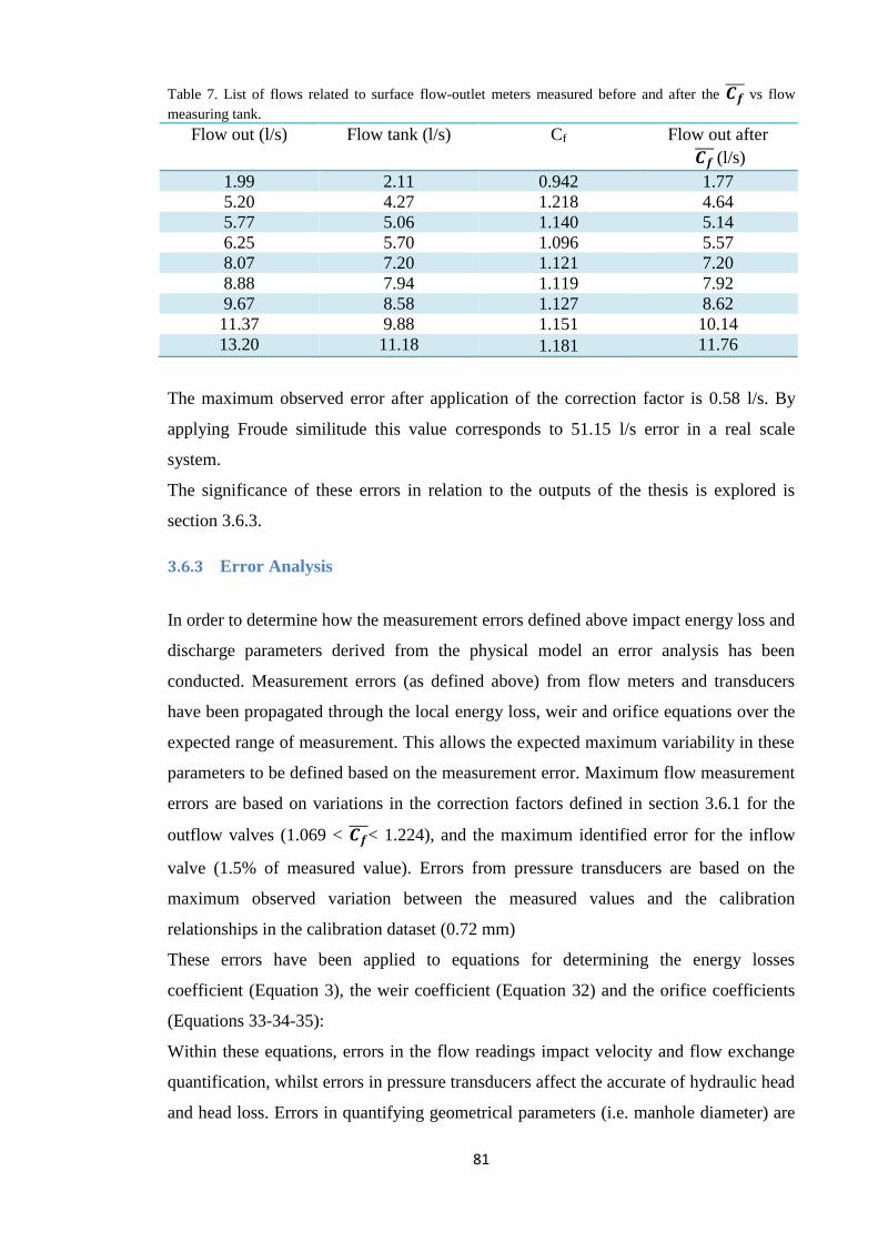
81
Table 7. List of flows related to surface flow-outlet meters measured before and after the 𝑪𝒇̅̅ ̅ vs flow
measuring tank.
Flow out (l/s) Flow tank (l/s) Cf Flow out after
𝑪𝒇̅̅ ̅ (l/s)
1.99 2.11 0.942 1.77
5.20 4.27 1.218 4.64
5.77 5.06 1.140 5.14
6.25 5.70 1.096 5.57
8.07 7.20 1.121 7.20
8.88 7.94 1.119 7.92
9.67 8.58 1.127 8.62
11.37 9.88 1.151 10.14
13.20 11.18 1.181 11.76
The maximum observed error after application of the correction factor is 0.58 l/s. By
applying Froude similitude this value corresponds to 51.15 l/s error in a real scale
system.
The significance of these errors in relation to the outputs of the thesis is explored is
section 3.6.3.
3.6.3 Error Analysis
In order to determine how the measurement errors defined above impact energy loss and
discharge parameters derived from the physical model an error analysis has been
conducted. Measurement errors (as defined above) from flow meters and transducers
have been propagated through the local energy loss, weir and orifice equations over the
expected range of measurement. This allows the expected maximum variability in these
parameters to be defined based on the measurement error. Maximum flow measurement
errors are based on variations in the correction factors defined in section 3.6.1 for the
outflow valves (1.069 < 𝑪𝒇̅̅ ̅< 1.224), and the maximum identified error for the inflow
valve (1.5% of measured value). Errors from pressure transducers are based on the
maximum observed variation between the measured values and the calibration
relationships in the calibration dataset (0.72 mm)
These errors have been applied to equations for determining the energy losses
coefficient (Equation 3), the weir coefficient (Equation 32) and the orifice coefficients
(Equations 33-34-35):
Within these equations, errors in the flow readings impact velocity and flow exchange
quantification, whilst errors in pressure transducers affect the accurate of hydraulic head
and head loss. Errors in quantifying geometrical parameters (i.e. manhole diameter) are

82
considered negligible. Applying the errors identified to each equation, the results of the
error analysis are presented in table 8. Both the range of errors and the average error
over the experimental range are presented.
Error values displayed confirm the accuracy of the energy losses and orifice coefficients
determined by the facility. Most existing studies do not report error values due to
measurement error, however the error values reported imply a higher accuracy then, for
example, Marsalek (1984) who reported 95% confidence limits (K values were found in
the range 0.102 to 0.344 in square shaped manholes, and 0.124 to 0.221 in circular
manholes) in reported K values. The average error is higher when estimating the weir
coefficients (0.13) and this can be explained by the occurrence of a siphon effect when
simulating surface to sewer exchange. A siphon effect occurs when the tube or pipe
through which a liquid is moving is affected by atmospheric pressure. This can act to
force liquid up an outlet due to the weight the liquid in another part of the system.
Unfortunately this could not be rectified within the tests conducted in this thesis, but can
be eliminated by installation of an additional pipe downstream exposed to atmospheric
pressure.

83
Table 8. Potential error in head loss and exchange equations coefficients over experimental range
Equation 𝑲𝒊 =
∆𝑯𝒊𝑽𝟐𝟐𝒈⁄
𝑪𝒘 =𝑸𝒆
𝟐𝟑∗ (𝟐𝒈)𝟎.𝟓 ∗ 𝒘 ∗ (∆𝑯𝒊)
𝟏.𝟓
𝑪𝒐 =𝑸𝒆
𝑨(𝟐𝒈∆𝑯𝒊)𝟎.𝟓
(orifice with no additional
flow on surface)
𝑪𝒐 =𝑸𝒆
𝑨(𝟐𝒈∆𝑯𝒊)𝟎.𝟓
(orifice with additional flow
on surface)
Experimental
range
4<Q<11.5 (l/s)
0.0035<∆𝐻𝑖<0.248 (m)
1.10<Qe<1.71 (l/s)
0.01<∆𝐻𝑖<0.013 (m)
0.62 < Qe < 4.67 (l/s)
0.098<∆𝐻𝑖<0. 293 (m)
1.26 < Qe < 5.50 (l/s)
0.045<∆𝐻𝑖<0.311 (m)
Range of error
in coefficient
over
experimental
range
0.0033-0.0051 0.11-0.145 0.00013-0.00015 0.00014-0.00066
Average error
over
experimental
range
0.0045 0.13 0.00014 0.00028

84
4 Pipe Network Results
The aim of this chapter is to detail the experiments conducted on the pipe network
described in section 3 which can be summarized in two categories, steady and unsteady
flow conditions. Tests conducted in steady flow conditions were used to define head
losses through the system under a range of high flow conditions (hence meeting
research objective 1). Tests conducted in unsteady conditions were used to evaluate
existing computer modelling tools, and identify the significance of local losses due to
manholes (hence meeting research objective 2).
4.1 Steady flow tests in the pipe network system
These tests have been used to characterize the response of the model to steady flow
conditions and to provide a complete hydraulic description of the performance of the
entire system including head losses through manhole structures.
A range of steady flow tests have been run using specific combinations of inflows
controlled via the inflow valves (tables 20-41). Appendix A displays the configuration
and the hydraulic conditions for each test, in terms of flow rate for each branch and
recorded water depths in Manhole 1, 2, 3, 4 (presented in figure 24).
4.2 Secondary losses
After having assessed the basic hydraulic components within the facility and the
frictional losses in the pipes, energy losses at manholes (which depend on flow rate,
junction geometry, change in flow direction, change in pipe elevation and the change in
pipe diameter between the inflow and outflow lines, Wang et al., 1998) have been
calculated under a range of steady flow conditions in order to meet research objective 1.
Pipes were fully pressurized in all tests conducted. The experimental tests conducted are
summarized in table 9, full details are provided in appendix A.
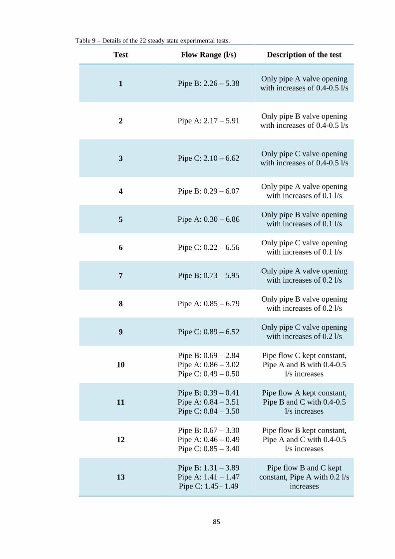
85
Table 9 – Details of the 22 steady state experimental tests.
Test Flow Range (l/s) Description of the test
1 Pipe B: 2.26 – 5.38 Only pipe A valve opening
with increases of 0.4-0.5 l/s
2 Pipe A: 2.17 – 5.91 Only pipe B valve opening
with increases of 0.4-0.5 l/s
3 Pipe C: 2.10 – 6.62 Only pipe C valve opening
with increases of 0.4-0.5 l/s
4 Pipe B: 0.29 – 6.07 Only pipe A valve opening
with increases of 0.1 l/s
5 Pipe A: 0.30 – 6.86 Only pipe B valve opening
with increases of 0.1 l/s
6 Pipe C: 0.22 – 6.56 Only pipe C valve opening
with increases of 0.1 l/s
7 Pipe B: 0.73 – 5.95 Only pipe A valve opening
with increases of 0.2 l/s
8 Pipe A: 0.85 – 6.79 Only pipe B valve opening
with increases of 0.2 l/s
9 Pipe C: 0.89 – 6.52 Only pipe C valve opening
with increases of 0.2 l/s
10
Pipe B: 0.69 – 2.84
Pipe A: 0.86 – 3.02
Pipe C: 0.49 – 0.50
Pipe flow C kept constant,
Pipe A and B with 0.4-0.5
l/s increases
11
Pipe B: 0.39 – 0.41
Pipe A: 0.84 – 3.51
Pipe C: 0.84 – 3.50
Pipe flow A kept constant,
Pipe B and C with 0.4-0.5
l/s increases
12
Pipe B: 0.67 – 3.30
Pipe A: 0.46 – 0.49
Pipe C: 0.85 – 3.40
Pipe flow B kept constant,
Pipe A and C with 0.4-0.5
l/s increases
13
Pipe B: 1.31 – 3.89
Pipe A: 1.41 – 1.47
Pipe C: 1.45– 1.49
Pipe flow B and C kept
constant, Pipe A with 0.2 l/s
increases
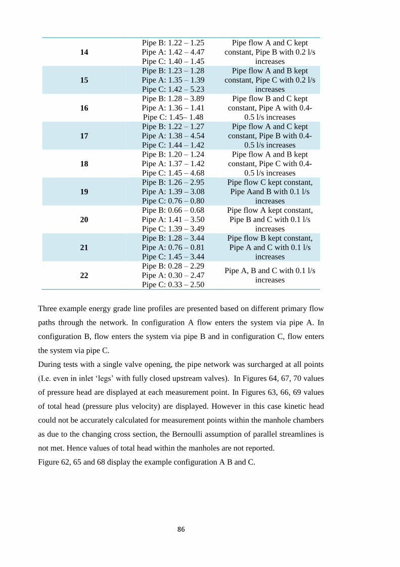
86
14
Pipe B: 1.22 – 1.25
Pipe A: 1.42 – 4.47
Pipe C: 1.40 – 1.45
Pipe flow A and C kept
constant, Pipe B with 0.2 l/s
increases
15
Pipe B: 1.23 – 1.28
Pipe A: 1.35 – 1.39
Pipe C: 1.42 – 5.23
Pipe flow A and B kept
constant, Pipe C with 0.2 l/s
increases
16
Pipe B: 1.28 – 3.89
Pipe A: 1.36 – 1.41
Pipe C: 1.45– 1.48
Pipe flow B and C kept
constant, Pipe A with 0.4-
0.5 l/s increases
17
Pipe B: 1.22 – 1.27
Pipe A: 1.38 – 4.54
Pipe C: 1.44 – 1.42
Pipe flow A and C kept
constant, Pipe B with 0.4-
0.5 l/s increases
18
Pipe B: 1.20 – 1.24
Pipe A: 1.37 – 1.42
Pipe C: 1.45 – 4.68
Pipe flow A and B kept
constant, Pipe C with 0.4-
0.5 l/s increases
19
Pipe B: 1.26 – 2.95
Pipe A: 1.39 – 3.08
Pipe C: 0.76 – 0.80
Pipe flow C kept constant,
Pipe Aand B with 0.1 l/s
increases
20
Pipe B: 0.66 – 0.68
Pipe A: 1.41 – 3.50
Pipe C: 1.39 – 3.49
Pipe flow A kept constant,
Pipe B and C with 0.1 l/s
increases
21
Pipe B: 1.28 – 3.44
Pipe A: 0.76 – 0.81
Pipe C: 1.45 – 3.44
Pipe flow B kept constant,
Pipe A and C with 0.1 l/s
increases
22
Pipe B: 0.28 – 2.29
Pipe A: 0.30 – 2.47
Pipe C: 0.33 – 2.50
Pipe A, B and C with 0.1 l/s
increases
Three example energy grade line profiles are presented based on different primary flow
paths through the network. In configuration A flow enters the system via pipe A. In
configuration B, flow enters the system via pipe B and in configuration C, flow enters
the system via pipe C.
During tests with a single valve opening, the pipe network was surcharged at all points
(I.e. even in inlet ‘legs’ with fully closed upstream valves). In Figures 64, 67, 70 values
of pressure head are displayed at each measurement point. In Figures 63, 66, 69 values
of total head (pressure plus velocity) are displayed. However in this case kinetic head
could not be accurately calculated for measurement points within the manhole chambers
as due to the changing cross section, the Bernoulli assumption of parallel streamlines is
not met. Hence values of total head within the manholes are not reported.
Figure 62, 65 and 68 display the example configuration A B and C.
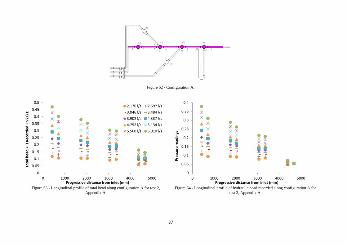
87
Figure 62 - Configuration A.
Figure 63 - Longitudinal profile of total head along configuration A for test 2,
Appendix A. Figure 64 - Longitudinal profile of hydraulic head recorded along configuration A for
test 2, Appendix A.
0
0.05
0.1
0.15
0.2
0.25
0.3
0.35
0.4
0.45
0.5
0 1000 2000 3000 4000 5000
Tota
l he
ad =
H R
eco
rde
d +
V2
/2g
Progressive distance from inlet (mm)
2.176 l/s 2.597 l/s
3.046 l/s 3.484 l/s
3.902 l/s 4.337 l/s
4.752 l/s 5.134 l/s
5.560 l/s 5.910 l/s
0
0.05
0.1
0.15
0.2
0.25
0.3
0.35
0.4
0 1000 2000 3000 4000 5000P
ress
ure
re
adin
gs
Progressive distance from inlet (mm)
88
Figure 65 – Configuration B.
Figure 66 - Longitudinal profile of total head along configuration B for test 1, Appendix
A.
Figure 67 - Longitudinal profile of hydraulic head recorded along configuration B for
test 1, Appendix A.
0
0.05
0.1
0.15
0.2
0.25
0.3
0.35
0.4
0.45
0.5
0 1000 2000 3000 4000 5000 6000
Tota
l He
ad =
H R
eco
rde
d +
V2
/2g
Progressive distance from inlet (mm)
2.265 l/s 2.689 l/s
3.114 l/s 3.536 l/s
4.146 l/s 4.533 l/s
5.023 l/s 5.384 l/s
0
0.05
0.1
0.15
0.2
0.25
0.3
0.35
0.4
0.45
0 1000 2000 3000 4000 5000 6000P
ress
ure
re
adin
gs
Progressive distance from inlet (mm)
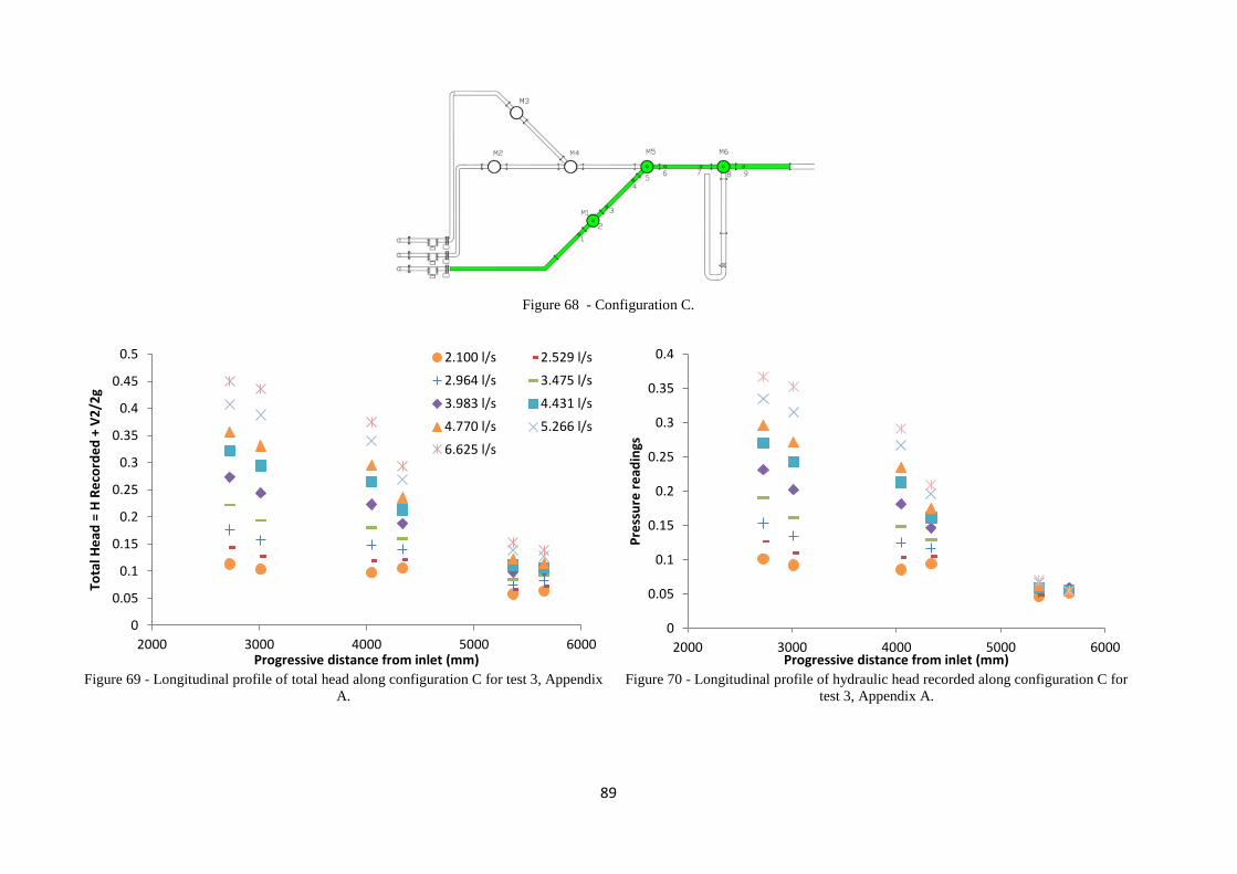
89
Figure 68 - Configuration C.
Figure 69 - Longitudinal profile of total head along configuration C for test 3, Appendix
A.
Figure 70 - Longitudinal profile of hydraulic head recorded along configuration C for
test 3, Appendix A.
0
0.05
0.1
0.15
0.2
0.25
0.3
0.35
0.4
0.45
0.5
2000 3000 4000 5000 6000
Tota
l He
ad =
H R
eco
rde
d +
V2
/2g
Progressive distance from inlet (mm)
2.100 l/s 2.529 l/s
2.964 l/s 3.475 l/s
3.983 l/s 4.431 l/s
4.770 l/s 5.266 l/s
6.625 l/s
0
0.05
0.1
0.15
0.2
0.25
0.3
0.35
0.4
2000 3000 4000 5000 6000P
ress
ure
re
adin
gs
Progressive distance from inlet (mm)
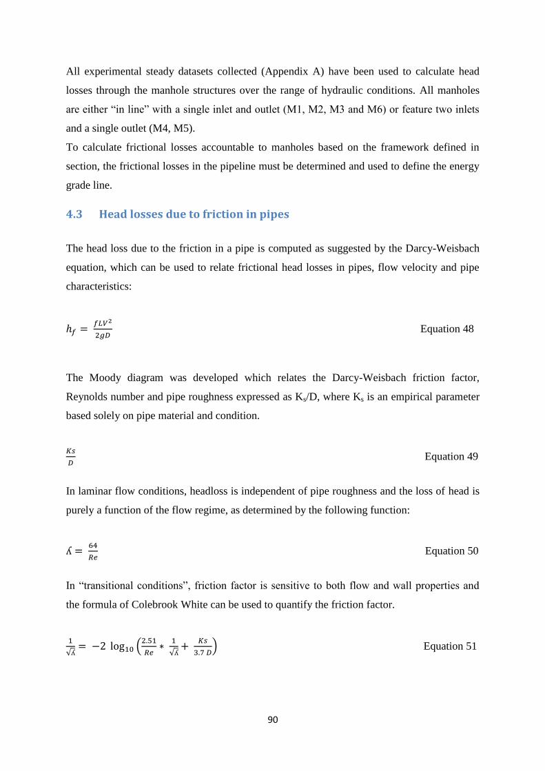
90
All experimental steady datasets collected (Appendix A) have been used to calculate head
losses through the manhole structures over the range of hydraulic conditions. All manholes
are either “in line” with a single inlet and outlet (M1, M2, M3 and M6) or feature two inlets
and a single outlet (M4, M5).
To calculate frictional losses accountable to manholes based on the framework defined in
section, the frictional losses in the pipeline must be determined and used to define the energy
grade line.
4.3 Head losses due to friction in pipes
The head loss due to the friction in a pipe is computed as suggested by the Darcy-Weisbach
equation, which can be used to relate frictional head losses in pipes, flow velocity and pipe
characteristics:
ℎ𝑓 = 𝑓𝐿𝑉2
2𝑔𝐷 Equation 48
The Moody diagram was developed which relates the Darcy-Weisbach friction factor,
Reynolds number and pipe roughness expressed as Ks/D, where Ks is an empirical parameter
based solely on pipe material and condition.
𝐾𝑠
𝐷 Equation 49
In laminar flow conditions, headloss is independent of pipe roughness and the loss of head is
purely a function of the flow regime, as determined by the following function:
ʎ = 64
𝑅𝑒 Equation 50
In “transitional conditions”, friction factor is sensitive to both flow and wall properties and
the formula of Colebrook White can be used to quantify the friction factor.
1
√ʎ= −2 log10 (
2.51
𝑅𝑒∗
1
√ʎ+
𝐾𝑠
3.7 𝐷) Equation 51

91
For smooth turbulent flow, wall roughness is fully covered by the viscous laminar sublayer
hence in that regime roughness does not influence friction losses. Therefore, the friction
factor equation becomes:
1
√ʎ= −2 log10 (
2.51
𝑅𝑒∗
1
√ʎ) Equation 52
In rough turbulent flow, the full Colebrook White equation applies, however friction factor
becomes insensitive to Reynolds number and can be written as:
1
√ʎ= −2 log10 (
𝐾𝑠
3.7 𝐷) Equation 53
Considering the experimental facility developed at the University of Sheffield, to determine
frictional losses inside the physical model pipe network, a range of flow tests inside a simple
length of pipe downstream of the manhole (Figure 71) were conducted and pressure drop
along a single pipe section (between PMDown 1 and PMDown 2) was related to flow
Reynolds No.
Figure 71 – Scheme of simple length pipe downstream of manhole used to characterize pipe frictional losses.
Table 10 – Hydraulic parameters within the experimental facility.
Test Flow (l/s) Pipe Flow
Velocity (m/s) Reynolds No.
1 4.364 0.99 73983
2 7.040 1.59 119335
3 8.213 1.86 139219
4 9.025 2.04 152983
5 9.604 2.17 162797
Manhole
P M
Down 2
P M
Down 1 P M
Down
0.35 m 0.50 m 4.15 m
P M Up
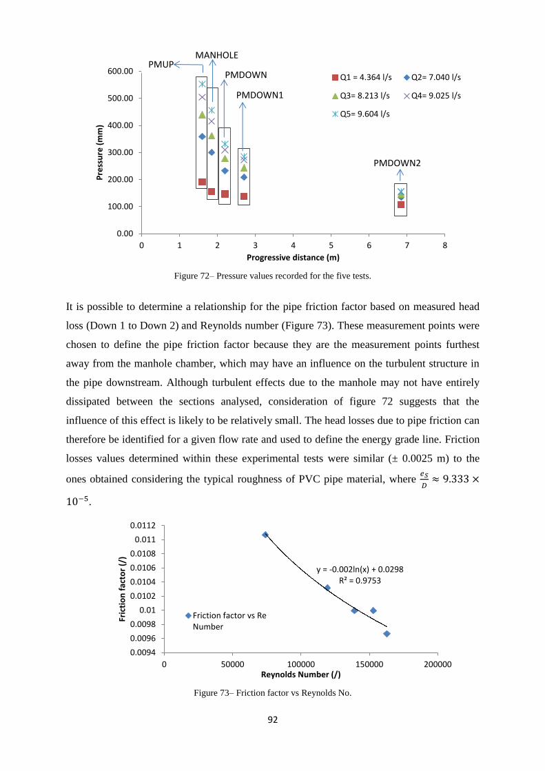
92
Figure 72– Pressure values recorded for the five tests.
It is possible to determine a relationship for the pipe friction factor based on measured head
loss (Down 1 to Down 2) and Reynolds number (Figure 73). These measurement points were
chosen to define the pipe friction factor because they are the measurement points furthest
away from the manhole chamber, which may have an influence on the turbulent structure in
the pipe downstream. Although turbulent effects due to the manhole may not have entirely
dissipated between the sections analysed, consideration of figure 72 suggests that the
influence of this effect is likely to be relatively small. The head losses due to pipe friction can
therefore be identified for a given flow rate and used to define the energy grade line. Friction
losses values determined within these experimental tests were similar (± 0.0025 m) to the
ones obtained considering the typical roughness of PVC pipe material, where 𝑒𝑆
𝐷≈ 9.333 ×
10−5.
Figure 73– Friction factor vs Reynolds No.
0.00
100.00
200.00
300.00
400.00
500.00
600.00
0 1 2 3 4 5 6 7 8
Pre
ssu
re (
mm
)
Progressive distance (m)
Q1 = 4.364 l/s Q2= 7.040 l/s
Q3= 8.213 l/s Q4= 9.025 l/s
Q5= 9.604 l/s
y = -0.002ln(x) + 0.0298 R² = 0.9753
0.0094
0.0096
0.0098
0.01
0.0102
0.0104
0.0106
0.0108
0.011
0.0112
0 50000 100000 150000 200000
Fric
tio
n f
acto
r (/
)
Reynolds Number (/)
Friction factor vs ReNumber
MANHOLE
PMDOWN
PMDOWN1
PMDOWN2
PMUP

93
4.4 “In line” manholes
As the slope of the facility is zero, head loss through attributable to each in line manhole is
calculated as measured head loss less the expected head loss in a straight pipe of equivalent
length due to friction:
ℎ𝐿 = [(𝐻𝑢𝑝) − (𝐻𝑑)] −𝑓𝐿𝑉2
2𝑔𝐷 Equation 54
Hup and Hd for each manhole can be obtained directly from the pressure readings upstream
and downstream of each manhole. In this case, due to constant pipe diameters upstream and
downstream of each manhole (and hence constant velocity head), only pressure head is
considered in equation 54. Pressure transducers are located 25 cm upstream and 35 cm
downstream of the manhole centerline in each case (hence the length, L in equation 54, of
the equivalent pipe is taken as 84 cm). Mean pipe velocity for the calculation of frictional
losses is obtained by dividing flow rate by pipe cross sectional area. The corresponding head-
loss coefficients K for each manhole have then been determined using equation 3. Figure 74
relates calculated head loss (from equation 54) for each ‘in line’ the manhole to velocity
head. The resulting best fit coefficients are presented in table 11.
Figure 74– Head losses manhole “in line”.
y (M2) = 0.3785x + 0.0055 R² = 0.99
y (M6) = 0.1704x - 0.0121 R² = 0.9415
y (M3) = 0.5184x + 0.0141 R² = 0.9927
y (M1) = 0.5763x + 0.0165 R² = 0.9855
0
0.01
0.02
0.03
0.04
0.05
0.06
0.07
0.08
0.09
0 0.02 0.04 0.06 0.08 0.1 0.12 0.14
hL
(m)
Vo2/2g (m)
M2M6M3M1

94
Table 11 – K values for ‘in line manholes’.
Manhole M1 M2 M3 M6
Coefficient (K) 0.57 0.37 0.51 0.17
The study has confirmed the proportionality of head losses at straight manholes to the
velocity head. Head loss coefficients for ‘in line’ manholes M2 and M6 in the central pipe
calculated by combining multiple steady flow configurations can be considered close to the
range 0.195-0.221 in literature for head loss through a straight manhole (Marsalek, 1984).
The value of K may be lower for M6 than M2 due to the enlargement on the outlet pipe
immediately downstream the final manhole of the system, where the diameter of the pipe
increases to 100 mm.
For manholes M1 and M3, K values are slightly higher than expected. This may be explained
by the 135 degree pipe bends immediately upstream of the manholes which may cause
irregular flow patterns inside the manhole inlet pipe, influencing the flow patterns inside the
manhole, and increasing the energy losses. The same justification has been given to justify
the non-perfect linear trend obtained by the values recorded, even if trend lines acquired
show good agreement for manhole M1 (R2=0.985) and M3 (R
2=0.992). The experiments
conducted demonstrate the high variability of K values and the sensitivity to upstream and
downstream pipe and flow conditions.
Another significant difference with previous studies is the presence of several manholes in
series. All previous studies have reported results for a single manhole. For example, the
energy losses generated by the configuration reported in Marsalek (1985) are caused only by
the main body of the stream crossing the single manhole. For the experimental facility
reported here each manhole is followed by another manhole and this could lead to additional
turbulence and associated energy losses. Some variability between observed values and those
found in the literature may also be explained by the presence of ‘still’ water in the pipe
network during test when only one upstream valve is open.

95
4.5 Energy Losses Through Manholes with Multiple inlets
Predictions for the energy loss coefficients have been made by applying the framework
described in section 2.5 (Zhao et al., 2006 and Pfister et al., (2014) and have been compared
with experimental data collected from the facility. Energy loss values presented here are
defined as those detailed in equations 9 and 10.
Relationships presented in section 2.4 have been applied to different flow combinations
through the experimental facility. Water was running through the pipes which were full (i.e.
pressurized flow).
Energy loss coefficients comparisons have been made between predictions and experimental
data for manhole 4 which is most hydraulically similar (if considered separated from the
entire system) to hydraulic models previously used. Comparisons were not completed for
manhole 5 because this junction is affected both by upstream and downstream conditions,
which are different from inlet and outlet conditions used by Zhao et al., (2006) and Pfister et
al., (2014). K12, K13 and Total K values as a function of relative flow in the inflow pipes are
presented in figure 75, alongside predictions made using the relationship defined by Zhao
(2006), i.e. equation 9-10.
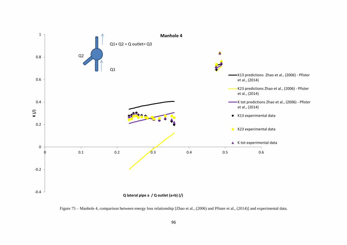
96
Figure 75 – Manhole 4, comparison between energy loss relationship [Zhao et al., (2006) and Pfister et al., (2014)] and experimental data.
-0.4
-0.2
0
0.2
0.4
0.6
0.8
1
0 0.1 0.2 0.3 0.4 0.5 0.6
K (
/)
Q lateral pipe a / Q outlet (a+b) (/)
Manhole 4
K13 predictions Zhao et al., (2006) - Pfisteret al., (2014)
K23 predictions Zhao et al., (2006) - Pfisteret al., (2014)
K tot predictions Zhao et al., (2006) - Pfisteret al., (2014)
K13 experimental data
K23 experimental data
K tot experimental data
Q1+ Q2 = Q outlet= Q3
Q1
Q2

97
It should be noted that, previous research (sections 2.3, 2.4, 2.5), has not used directly
comparable geometries to that in the current facility, hence it is difficult to identify if
these findings are in direct agreement with previous work, Zhao et al., (2006) and
Pfister et al., (2014).
Despite this, the results show interesting similarities between experimental data and
energy losses coefficients defined by equation 9-10 for Qlateral/Qoutlet = 0.5. For
Qlateral/Qoutlet = 0.22-0.36 comparisons have shown the predictions obtained using the
model of Zhao et al., 2006, overestimate the energy loss coefficients K23 and
underestimate the energy loss coefficients K13. However overall, this means that the
predictions for the total K are reasonably accurate (with 6.8%). Discrepancies in terms
of predicted trends using equation 9-10 are also evident. These comparisons have
highlighted the significance of flow streamlines created inside the manholes under
different flow combinations on energy losses coefficients. Having more complex flow
patterns generates more effects on energy losses due to retardation, acceleration,
rotation in different planes and flow interference.
4.6 Quantification of hydraulic capacity of the sewer system
The number of times the flow breached a defined level in the manholes during all the
steady tests was also recorded. The threshold level was selected as 430 mm, dependent
on the number of valve opening and on the magnitude of flow rate, therefore primary
decision of the controller to stop the simulation during the tests.
The results are presented in figure 76:
Figure 76– Flooding times.
It is possible to notice that the bigger risk of flooding comes from the manhole 2,
followed by manhole 3 and then 1 and 4.
0
2
4
6
8
10
12
14
Manhole 1Manhole 2Manhole 3Manhole 4Manhole 5Manhole 6
N. o
f ti
me
s cl
ose
to
fl
oo
din
g w
ith
in t
he
22
e
xpe
rim
en
ts p
rese
nte
d in
A
pp
en
dix
A

98
For each simulation the maximum flow contained by the system has been calculated and
figure 76 displays the overall values.
The maximum flow reached through branch A was 6.072 l/s.
The maximum flow reached in the branch B was 6.975 l/s.
The maximum flow achieved in branch C corresponds to 6.564 l/s.
Figure 77 - Total flow for each simulation.
4.7 Scaled Rainfall Event Simulations
Having characterized the steady state system, a number of unsteady flow events were
conducted. The flow hydrographs tested were based on real storm events measured in an
urban catchment in the north of England, scaled to the experimental facility. The overall
aim of these tests was to provide datasets that could be used to calibrate and validate
sewer flow models including the commercial model Infoworks as well as the SIPSON
model provided by collaborators at the University of Coimbra, as well as identify the
significance of local head losses (research objective 2). However initial tests conducted
were focused on identifying if the scaled physical model could reproduce hydraulic
phenomena as observed in a full scale system.
For these initial tests, unsteady flow input hydrographs were based on rainfall events
measured by using a rain gauge from a site. The data was provided by Yorkshire Water
Services, and converted into sewer inflow hydrographs using empirical rainfall-runoff
relationships as utilised within commercial Infoworks software. These hydrographs
5.00
5.50
6.00
6.50
7.00
7.50
8.00
Tota
l flo
w (
l/s)
Test
1 2 3 4 5 6 7 8 9 10 11
12 13 14 15 16 17 18 19 20 21 22
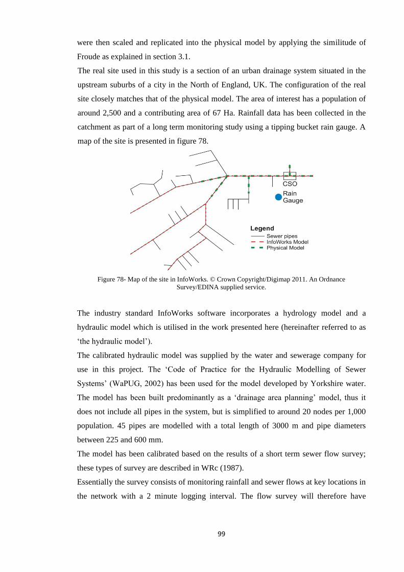
99
were then scaled and replicated into the physical model by applying the similitude of
Froude as explained in section 3.1.
The real site used in this study is a section of an urban drainage system situated in the
upstream suburbs of a city in the North of England, UK. The configuration of the real
site closely matches that of the physical model. The area of interest has a population of
around 2,500 and a contributing area of 67 Ha. Rainfall data has been collected in the
catchment as part of a long term monitoring study using a tipping bucket rain gauge. A
map of the site is presented in figure 78.
Figure 78- Map of the site in InfoWorks. © Crown Copyright/Digimap 2011. An Ordnance
Survey/EDINA supplied service.
The industry standard InfoWorks software incorporates a hydrology model and a
hydraulic model which is utilised in the work presented here (hereinafter referred to as
‘the hydraulic model’).
The calibrated hydraulic model was supplied by the water and sewerage company for
use in this project. The ‘Code of Practice for the Hydraulic Modelling of Sewer
Systems’ (WaPUG, 2002) has been used for the model developed by Yorkshire water.
The model has been built predominantly as a ‘drainage area planning’ model, thus it
does not include all pipes in the system, but is simplified to around 20 nodes per 1,000
population. 45 pipes are modelled with a total length of 3000 m and pipe diameters
between 225 and 600 mm.
The model has been calibrated based on the results of a short term sewer flow survey;
these types of survey are described in WRc (1987).
Essentially the survey consists of monitoring rainfall and sewer flows at key locations in
the network with a 2 minute logging interval. The flow survey will therefore have

100
recorded 2 dry weather flow days and 3 rainfall events which meet criteria including
minimum flow depths, rainfall intensity, duration and limits on spatial variability.
The model available covers the entire city, but only a very small section relating to the
area of interest is described here because the aim was to find a site with similar
characteristics of the experimental model.
Considering that the physical model includes three inlet pipes with the addition of two
junctions, a specific analysis of the existing real model has been completed to find a
similar geometrical combination to use for a comparison between experimental and
physical results.
The area identified for the analysis is presented in figure 78 and includes three pipes
plus a CSO.
Input flow hydrographs for the physical and numerical models were based on rainfall
data (depth, intensity and duration) measured in the catchment using the rain gauge over
the period April 2008 - June 2009.
The events selected for the simulations (listed in table 12) were those recorded within
the catchment with durations of 15 ± 1, 30 ±2, 45 ±1 and 60 ± 2 minutes.
This period represents the typical range used for planning sewer systems. The rainfall
events were converted into runoff using the “new UK runoff equation” and the equation
for the time of entry as utilized in Infoworks. The Infoworks hydraulics were also used
to simulate sewer network flows upstream of the simulated area.
To determine hydrographs for each drained section of the catchment, Infoworks creates
a volume model to establish the volume generated from the rainfall event. Successively,
it produces a routine model calculating the flow generated within each subcatchment
which then can be used for simulations in the physical model.
A description of the simulation process using Infoworks has been omitted for brevity
but the interested reader is referred to WAPUG (Code of practice, 2002).
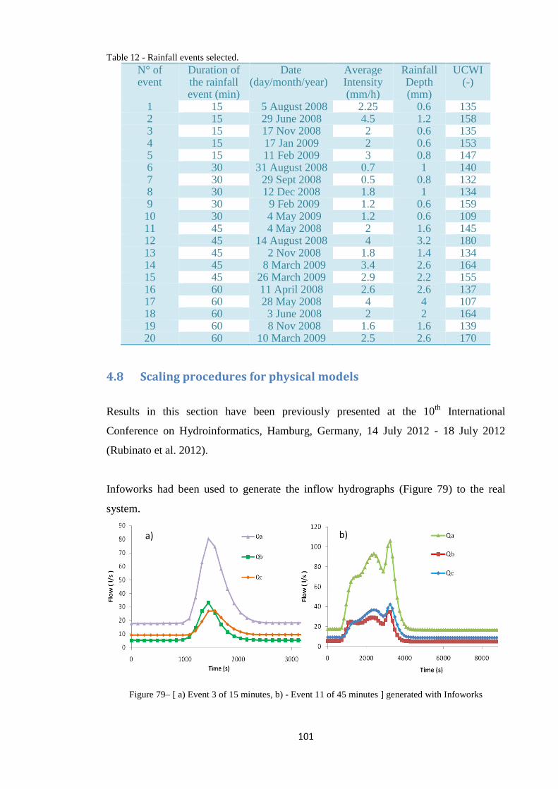
101
Table 12 - Rainfall events selected.
N° of event
Duration of the rainfall event (min)
Date (day/month/year)
Average Intensity (mm/h)
Rainfall Depth (mm)
UCWI (-)
1 15 5 August 2008 2.25 0.6 135 2 15 29 June 2008 4.5 1.2 158 3 15 17 Nov 2008 2 0.6 135 4 15 17 Jan 2009 2 0.6 153 5 15 11 Feb 2009 3 0.8 147 6 30 31 August 2008 0.7 1 140 7 30 29 Sept 2008 0.5 0.8 132 8 30 12 Dec 2008 1.8 1 134 9 30 9 Feb 2009 1.2 0.6 159 10 30 4 May 2009 1.2 0.6 109 11 45 4 May 2008 2 1.6 145 12 45 14 August 2008 4 3.2 180 13 45 2 Nov 2008 1.8 1.4 134 14 45 8 March 2009 3.4 2.6 164 15 45 26 March 2009 2.9 2.2 155 16 60 11 April 2008 2.6 2.6 137 17 60 28 May 2008 4 4 107 18 60 3 June 2008 2 2 164 19 60 8 Nov 2008 1.6 1.6 139 20 60 10 March 2009 2.5 2.6 170
4.8 Scaling procedures for physical models
Results in this section have been previously presented at the 10th
International
Conference on Hydroinformatics, Hamburg, Germany, 14 July 2012 - 18 July 2012
(Rubinato et al. 2012).
Infoworks had been used to generate the inflow hydrographs (Figure 79) to the real
system.
Figure 79– [ a) Event 3 of 15 minutes, b) - Event 11 of 45 minutes ] generated with Infoworks
a) b)
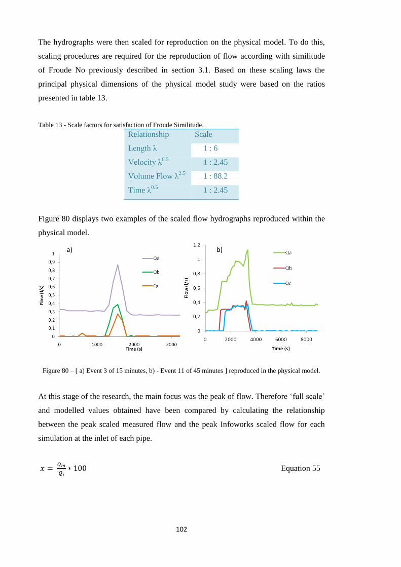
102
The hydrographs were then scaled for reproduction on the physical model. To do this,
scaling procedures are required for the reproduction of flow according with similitude
of Froude No previously described in section 3.1. Based on these scaling laws the
principal physical dimensions of the physical model study were based on the ratios
presented in table 13.
Table 13 - Scale factors for satisfaction of Froude Similitude.
Relationship Scale
Length λ 1 : 6
Velocity λ0.5
1 : 2.45
Volume Flow λ2.5
1 : 88.2
Time λ0.5
1 : 2.45
Figure 80 displays two examples of the scaled flow hydrographs reproduced within the
physical model.
Figure 80 – [ a) Event 3 of 15 minutes, b) - Event 11 of 45 minutes ] reproduced in the physical model.
At this stage of the research, the main focus was the peak of flow. Therefore ‘full scale’
and modelled values obtained have been compared by calculating the relationship
between the peak scaled measured flow and the peak Infoworks scaled flow for each
simulation at the inlet of each pipe.
𝑥 = 𝑄𝑚
𝑄𝑖∗ 100 Equation 55
b) a)
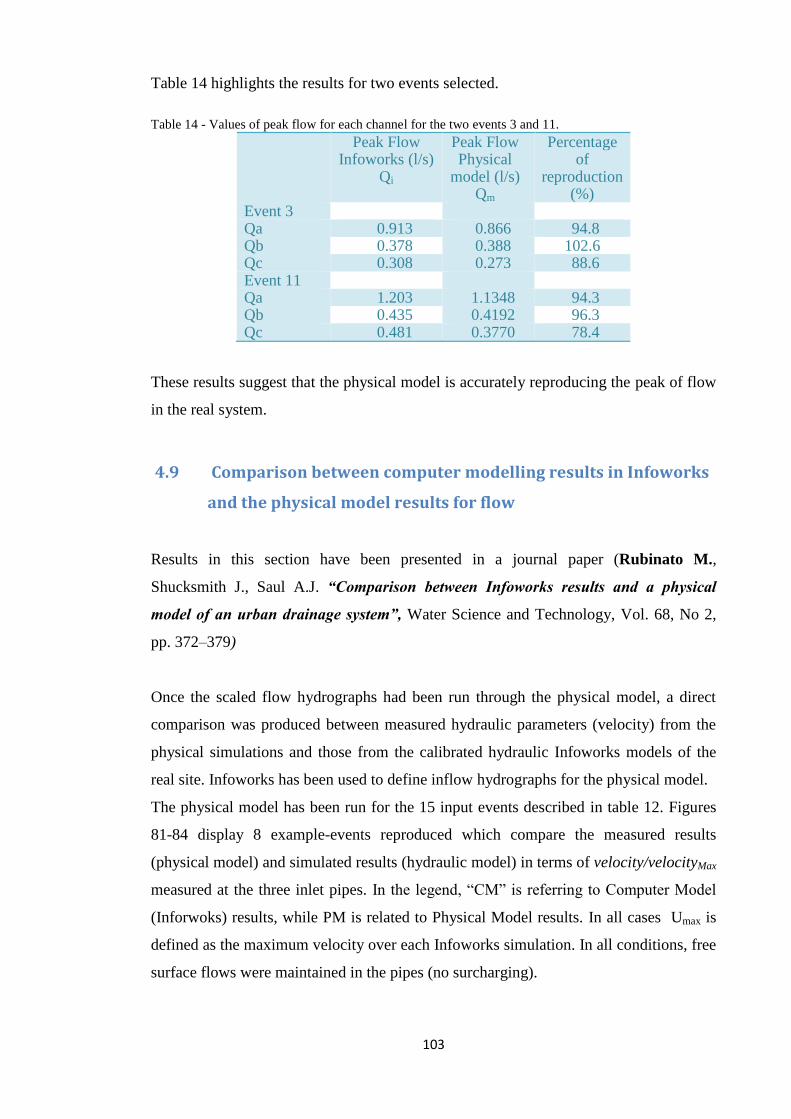
103
Table 14 highlights the results for two events selected.
Table 14 - Values of peak flow for each channel for the two events 3 and 11.
Peak Flow Infoworks (l/s)
Qi
Peak Flow Physical
model (l/s) Qm
Percentage of
reproduction (%)
Event 3 Qa 0.913 0.866 94.8 Qb 0.378 0.388 102.6 Qc 0.308 0.273 88.6 Event 11 Qa 1.203 1.1348 94.3 Qb 0.435 0.4192 96.3 Qc 0.481 0.3770 78.4
These results suggest that the physical model is accurately reproducing the peak of flow
in the real system.
4.9 Comparison between computer modelling results in Infoworks
and the physical model results for flow
Results in this section have been presented in a journal paper (Rubinato M.,
Shucksmith J., Saul A.J. “Comparison between Infoworks results and a physical
model of an urban drainage system”, Water Science and Technology, Vol. 68, No 2,
pp. 372–379)
Once the scaled flow hydrographs had been run through the physical model, a direct
comparison was produced between measured hydraulic parameters (velocity) from the
physical simulations and those from the calibrated hydraulic Infoworks models of the
real site. Infoworks has been used to define inflow hydrographs for the physical model.
The physical model has been run for the 15 input events described in table 12. Figures
81-84 display 8 example-events reproduced which compare the measured results
(physical model) and simulated results (hydraulic model) in terms of velocity/velocityMax
measured at the three inlet pipes. In the legend, “CM” is referring to Computer Model
(Inforwoks) results, while PM is related to Physical Model results. In all cases Umax is
defined as the maximum velocity over each Infoworks simulation. In all conditions, free
surface flows were maintained in the pipes (no surcharging).

104
Figure 81- Two selected events, Event 5 (11
th February 2009) and Event 3 (17
th November 2008), are
displayed. Both rainfall events are of 15 minutes duration.
Figure 82 - Two selected events, Event 10 (4th
May 2009) and Event 9 (9th
February 2009), are displayed.
Both rainfall events are of 30 minutes duration.
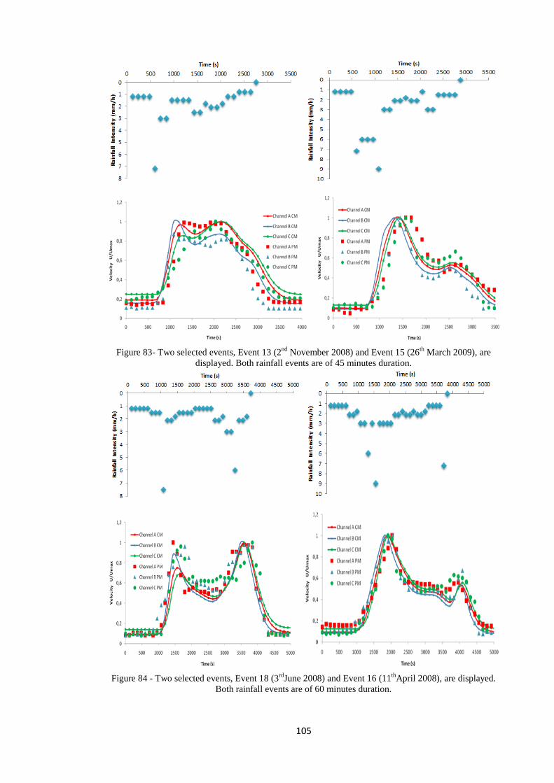
105
Figure 83- Two selected events, Event 13 (2nd
November 2008) and Event 15 (26th
March 2009), are
displayed. Both rainfall events are of 45 minutes duration.
Figure 84 - Two selected events, Event 18 (3rd
June 2008) and Event 16 (11th
April 2008), are displayed.
Both rainfall events are of 60 minutes duration.
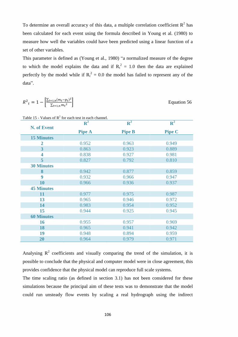
106
To determine an overall accuracy of this data, a multiple correlation coefficient R2 has
been calculated for each event using the formula described in Young et al. (1980) to
measure how well the variables could have been predicted using a linear function of a
set of other variables.
This parameter is defined as (Young et al., 1980) “a normalized measure of the degree
to which the model explains the data and if Rt2 = 1.0 then the data are explained
perfectly by the model while if Rt2 = 0.0 the model has failed to represent any of the
data”.
𝑅2𝑡 = 1 − [∑ (𝑚𝑡−𝑝𝑡)
2𝑡=1,𝑛
∑ 𝑚𝑡2𝑡=1,𝑛] Equation 56
Table 15 - Values of R2 for each test in each channel.
N. of Event R
2
Pipe A
R2
Pipe B
R2
Pipe C
15 Minutes
2 0.952 0.963 0.949
3 0.863 0.923 0.889
4 0.838 0.927 0.981
5 0.827 0.792 0.810
30 Minutes
8 0.942 0.877 0.859
9 0.932 0.966 0.947
10 0.966 0.936 0.937
45 Minutes
11 0.977 0.975 0.987
13 0.965 0.946 0.972
14 0.983 0.954 0.952
15 0.944 0.925 0.945
60 Minutes
16 0.955 0.957 0.969
18 0.965 0.941 0.942
19 0.948 0.894 0.959
20 0.964 0.979 0.971
Analysing R2 coefficients and visually comparing the trend of the simulation, it is
possible to conclude that the physical and computer model were in close agreement, this
provides confidence that the physical model can reproduce full scale systems.
The time scaling ratio (as defined in section 3.1) has not been considered for these
simulations because the principal aim of these tests was to demonstrate that the model
could run unsteady flow events by scaling a real hydrograph using the indirect

107
interpolation between valve openings and flow rates by subsequently applying the time
ratio scale.
Table 16 displays the duration of the tested storm events scaled by using the similitude
of Froude (1:6).
Table 16 – Time scales to satisfy the similitude of Froude within the physical model.
Time (min) Real System Time (min) Prototype –
Physical Model
15 6.12
30 12.25
45 18.37
60 24.49
The consideration of time scaling may be important for future studies as the turbulence
and the streamlines created inside the manhole may be different if flow rise or fall at
different rates, which may affect local energy losses. Therefore the time scaling ratio
will be considered for future studies. Based on Froude similitude, replicating real events
of 15, 30, 45 and 60 minutes will correspond to 6, 12, 18 and 24 minutes events in the
physical model. This is an important aspect to consider when designing Particle Image
Velocimetry (PIV) systems because the duration of the event simulated has to be related
with the time acquisitions of the cameras and the capacity of the hardware (Weitbrecht
et al., 2001 – Weitbrecht et al., 2002).
4.10 Flow conditions at network junctions
Results in this section have been previously presented at the 9th
International
Conference on Urban Drainage Modelling, Belgrade, Serbia, 3-8 September 2012 and
are under review for publication. The experimental part of this work and the associated
data presented has been collected and analysed by the author. The numerical analysis
and sewer network modelling described in this section has been conducted by
collaborators at the University of Coimbra, in particular by PhD student Nuno Melo.
The aim of this work was to compare the observed flow in a scale model of an urban
drainage system, with the results obtained using two one-dimensional (1D) numerical
models, SIPSON and SWMM, in order to validate the internal boundary conditions. The
calibration of the models was completed using the experimental data of the two storm
events occurred on 12th
December 2008 and 17th
January 2009 (data measured by a rain

108
gauge installed in the basin), thus validating the internal boundary conditions.
Infoworks was not used for this comparison because this model (i.e. the one developed
and made available by Yorkshire Water) was not an exact replica of the experimental
facility. In particular, the manhole angles and location in the infoworks model and the
physical model were not identical. In order to provide a more robust comparison
between computational and physical models it was necessary to build a model which
represented the physical model exactly. For this work two one-dimensional models,
SIPSON and SWMM were used.
SIPSON is a 1D/1D integrated hydraulic model developed by Djordjevic (2001) at the
University of Belgrade. The acronym SIPSON stands for “Simulation of Interaction
between Pipe flow and Overland flow in Networks”. SIPSON, besides being a hydraulic
model, also incorporates a hydrologic model (rainfall runoff), called BEMUS, which is
used for calculating the surface runoff input to the hydraulic model. A GIS interface,
named 3DNet, works as the platform for management and editing of data and
visualization of the SIPSON results. The hydraulic model solves simultaneously the
continuity equations for network nodes, the complete St. Venant equations for the 1D
network and the links equations (Djordjevic et al., 2005). The modelling of the manhole
head losses was done by considering local losses (∆H) for both the inlet and the outlet
of the manholes quantified through equations of the type ∆H=K(V2/2g) in which V is
the average velocity in the upstream pipe, and K is the head loss coefficient (which is to
be calibrated). Storm Water Management Model (SWMM) is a dynamic rainfall-runoff
model. The component of runoff operates on a collection of sub-catchment areas that
receive precipitation and generate runoff. The routing of the SWMM runoff is done
through the system of channels, pipes and devices. The flow routing in this case is
calculated, using the complete one-dimensional Saint Venant flow equations (Dynamic
Wave Routing) (Rossman, 2010). This routing method can account for channel storage,
backwater, entrance/exit losses, flow reversal, and pressurized flow (Rossman, 2010).
As in SIPSON, the head losses in the manholes are considered by introducing local loss
coefficients at entry and exit of each pipe.
In order to obtain consistent modelling results with SIPSON and SWMM, a calibration
process was applied. The selected calibration parameters included roughness of the pipe
and the local head losses at manholes. The computational model parameters where
adjusted such that the best possible fit was obtained between the computational and
physical model results for all the unsteady simulations tests (i.e. one set of calibration
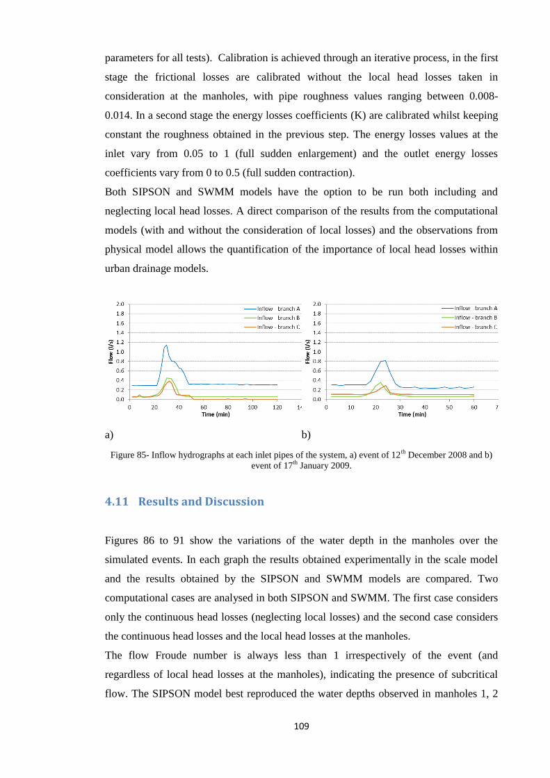
109
parameters for all tests). Calibration is achieved through an iterative process, in the first
stage the frictional losses are calibrated without the local head losses taken in
consideration at the manholes, with pipe roughness values ranging between 0.008-
0.014. In a second stage the energy losses coefficients (K) are calibrated whilst keeping
constant the roughness obtained in the previous step. The energy losses values at the
inlet vary from 0.05 to 1 (full sudden enlargement) and the outlet energy losses
coefficients vary from 0 to 0.5 (full sudden contraction).
Both SIPSON and SWMM models have the option to be run both including and
neglecting local head losses. A direct comparison of the results from the computational
models (with and without the consideration of local losses) and the observations from
physical model allows the quantification of the importance of local head losses within
urban drainage models.
a)
b)
Figure 85- Inflow hydrographs at each inlet pipes of the system, a) event of 12th
December 2008 and b)
event of 17th
January 2009.
4.11 Results and Discussion
Figures 86 to 91 show the variations of the water depth in the manholes over the
simulated events. In each graph the results obtained experimentally in the scale model
and the results obtained by the SIPSON and SWMM models are compared. Two
computational cases are analysed in both SIPSON and SWMM. The first case considers
only the continuous head losses (neglecting local losses) and the second case considers
the continuous head losses and the local head losses at the manholes.
The flow Froude number is always less than 1 irrespectively of the event (and
regardless of local head losses at the manholes), indicating the presence of subcritical
flow. The SIPSON model best reproduced the water depths observed in manholes 1, 2
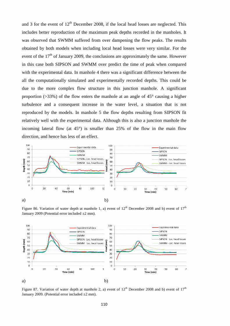
110
and 3 for the event of 12th
December 2008, if the local head losses are neglected. This
includes better reproduction of the maximum peak depths recorded in the manholes. It
was observed that SWMM suffered from over dampening the flow peaks. The results
obtained by both models when including local head losses were very similar. For the
event of the 17th
of January 2009, the conclusions are approximately the same. However
in this case both SIPSON and SWMM over predict the time of peak when compared
with the experimental data. In manhole 4 there was a significant difference between the
all the computationally simulated and experimentally recorded depths. This could be
due to the more complex flow structure in this junction manhole. A significant
proportion (>33%) of the flow enters the manhole at an angle of 45° causing a higher
turbulence and a consequent increase in the water level, a situation that is not
reproduced by the models. In manhole 5 the flow depths resulting from SIPSON fit
relatively well with the experimental data. Although this is also a junction manhole the
incoming lateral flow (at 45°) is smaller than 25% of the flow in the main flow
direction, and hence has less of an effect.
a)
b)
Figure 86. Variation of water depth at manhole 1, a) event of 12th
December 2008 and b) event of 17th
January 2009 (Potential error included ±2 mm).
a)
b)
Figure 87. Variation of water depth at manhole 2, a) event of 12th
December 2008 and b) event of 17th
January 2009. (Potential error included ±2 mm).
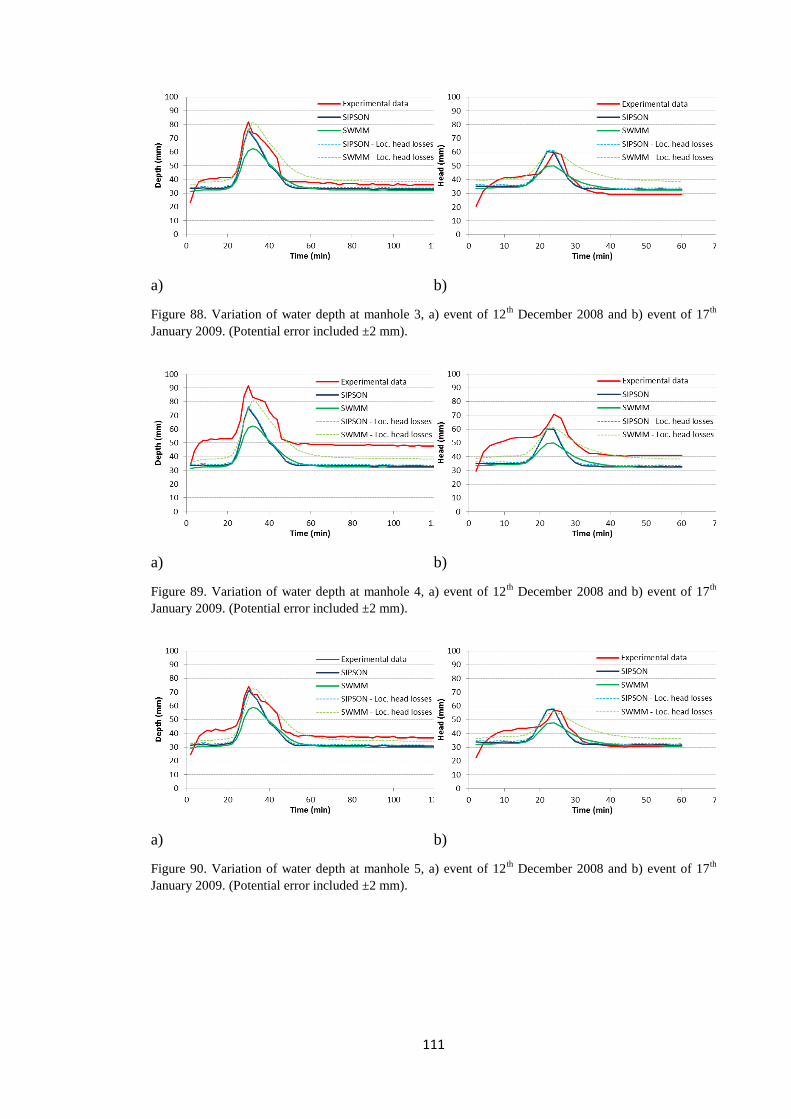
111
a)
b)
Figure 88. Variation of water depth at manhole 3, a) event of 12th
December 2008 and b) event of 17th
January 2009. (Potential error included ±2 mm).
a)
b)
Figure 89. Variation of water depth at manhole 4, a) event of 12th
December 2008 and b) event of 17th
January 2009. (Potential error included ±2 mm).
a)
b)
Figure 90. Variation of water depth at manhole 5, a) event of 12th
December 2008 and b) event of 17th
January 2009. (Potential error included ±2 mm).
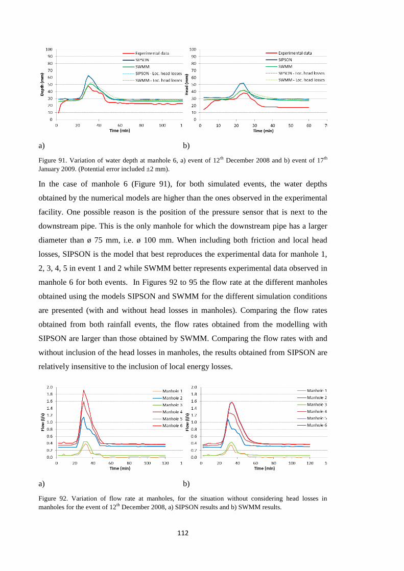
112
a)
b)
Figure 91. Variation of water depth at manhole 6, a) event of 12th
December 2008 and b) event of 17th
January 2009. (Potential error included ±2 mm).
In the case of manhole 6 (Figure 91), for both simulated events, the water depths
obtained by the numerical models are higher than the ones observed in the experimental
facility. One possible reason is the position of the pressure sensor that is next to the
downstream pipe. This is the only manhole for which the downstream pipe has a larger
diameter than ø 75 mm, i.e. ø 100 mm. When including both friction and local head
losses, SIPSON is the model that best reproduces the experimental data for manhole 1,
2, 3, 4, 5 in event 1 and 2 while SWMM better represents experimental data observed in
manhole 6 for both events. In Figures 92 to 95 the flow rate at the different manholes
obtained using the models SIPSON and SWMM for the different simulation conditions
are presented (with and without head losses in manholes). Comparing the flow rates
obtained from both rainfall events, the flow rates obtained from the modelling with
SIPSON are larger than those obtained by SWMM. Comparing the flow rates with and
without inclusion of the head losses in manholes, the results obtained from SIPSON are
relatively insensitive to the inclusion of local energy losses.
a)
b)
Figure 92. Variation of flow rate at manholes, for the situation without considering head losses in
manholes for the event of 12th
December 2008, a) SIPSON results and b) SWMM results.
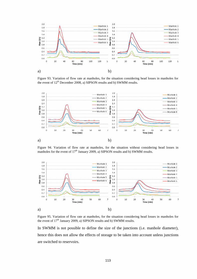
113
a)
b)
Figure 93. Variation of flow rate at manholes, for the situation considering head losses in manholes for
the event of 12th
December 2008, a) SIPSON results and b) SWMM results.
a)
b)
Figure 94. Variation of flow rate at manholes, for the situation without considering head losses in
manholes for the event of 17th
January 2009, a) SIPSON results and b) SWMM results.
a)
b)
Figure 95. Variation of flow rate at manholes, for the situation considering head losses in manholes for
the event of 17th
January 2009, a) SIPSON results and b) SWMM results.
In SWMM is not possible to define the size of the junctions (i.e. manhole diameter),
hence this does not allow the effects of storage to be taken into account unless junctions
are switched to reservoirs.

114
This could explain the differences found in the calibrated roughness parameter obtained
for the different models: after the calibration the value of roughness in SWMM are
slightly higher than in SIPSON in order to compensate for the damping of the peak
flows.
In summary, tests have shown that:
SWMM shows a higher peak damping than SIPSON;
For the first event, SWMM overshoots the time to peak when compared with
experimental data.
After calibration, the inclusion of head losses did not significantly improve the
overall performance of the computer models over the events tested.
Finally, it should also be mentioned that both models did not reproduce the start-up time
seen in the experimental facility. This could also be obtained in SWMM and SIPSON
but it would require a further calibration for a gradual input-curve that could simulate
the start-up time.
In conclusion hydraulic datasets obtained by the experimental facility have been utilized
to verify the accuracy of SWMM and SIPSON. When modelling the experimental
facility it was found that SIPSON reproduces fairly well the water depths in the
manholes of the drainage system when considering the friction head losses and the local
losses at the manholes.

115
5 Results of above/below ground physical model
This chapter presents the results obtained in the second phase of this research, with the
experimental apparatus as described in section 3. This includes the simulation of
different pluvial flooding scenarios in the experimental facility after the construction of
an urban surface on the top of the pipe network.
The aim of this phase of the research is to investigate flow exchange from sewer to
surface flows in flood events and investigate the applicability of weir and orifice linking
equations utilized in hydraulic flood models.
A subset of the results in this section has been previously presented at the 11th
HIC,
International Conference on Hydroinformatics, New York, USA, 17 August 2014- 21
August 2014.
5.1 Exchange below/above ground urban floods: steady flow
conditions
Within the physical model during flow events, flow exchange can be quantified via
mass balance equations using measured flow data at the facility inlets and outlets as
follows:
𝑄𝑒 = 𝑄1 − 𝑄3 = −𝑄2 + 𝑄4 Equation 57
Figure 96- Scheme of flow exchange.
116
Three different scenarios have been tested and investigated using the physical model:
1. Water running on the urban surface with no flow running into the pipes, to
quantify the flow exchange from the above system to the below system;
2. Water running through the pipes and surcharging onto the urban surface, with no
additional surface flow (i.e. Q2=0). To determine the flow exchange from the
below system to the above system with no surface water;
3. Water running through the pipes surcharging onto the urban surface, with
additional flow (i.e. Q2>0). To determine the flow exchange from the below
system to the above system in the presence of shallow surface flow.
As previously explained in section 2.7, according to the framework proposed by
Djordjevic and Chen, 2010, flow exchange is dependent on the relative head between
sewer and surface flow and is commonly modelled using weir and/or orifice equations.
Within the experimental model, pressure head within the below ground system can be
measured directly by the use of three pressure transducers, located respectively
upstream, downstream and inside the manhole. Pressure (depth) on the surface can be
measured using six pressure transducers: one located upstream the manhole, one
downstream with additional two on the right and two on the left to cover the entire area,
as displayed in figure 38.
Within this system datum is defined as the free surface bed level, 478 mm above the
pipe invert. Velocity at each point in the system can be calculated using mass
conservation principles and knowledge of inlet and outlet flows, pipe geometries and
free surface depths.
5.1.1 Scenario 1
Five tests have been conducted to replicate surface to sewer transfer with no pipe flow.
For each test, different parameters have been quantified as follows:
Head in pipe upstream of the manhole
𝐻𝑢𝑝, 𝑝 = 𝑃𝑢𝑝,𝑝
𝜌𝑔+
𝑉𝑢𝑝,𝑝2
2𝑔 Equation 58
Head in pipe downstream of the manhole

117
𝐻𝑑𝑜𝑤𝑛, 𝑝 = 𝑃𝑑𝑜𝑤𝑛,𝑝
𝜌𝑔+
𝑉𝑑𝑜𝑤𝑛,𝑝2
2𝑔 Equation 59
Head in surface upstream of the manhole (interface)
𝐻𝑢𝑝, 𝑠 = 𝑃𝑢𝑝,𝑠
𝜌𝑔+
𝑉𝑢𝑝,𝑠2
2𝑔+ 𝑧 Equation 60
Head in surface downstream of the manhole (interface)
𝐻𝑑𝑜𝑤𝑛, 𝑠 = 𝑃𝑑𝑜𝑤𝑛,𝑠
𝜌𝑔+
𝑉𝑑𝑜𝑤𝑛,𝑠2
2𝑔+ 𝑧 Equation 61
Total Head Losses, Ht (m)
(𝐻𝑢𝑝, 𝑝 + 𝐻𝑢𝑝, 𝑠) − (𝐻𝑑𝑜𝑤𝑛, 𝑝 + 𝐻𝑑𝑜𝑤𝑛, 𝑠) Equation 62
For determining kinetic energy in equation 58 and 59, the velocity is calculated using
the measured flow rate at the facility sewer inlet or outlet (respectively) and pipe cross-
section.
For determining kinetic energy in equation 60 and 61, the velocity is calculated using
the measured flow rate at the facility surface inlet or outlet (respectively) and open
channel cross-sectional area. Due to the width of the flume and the relatively low
exchange rates, the differences in the kinetic energy of the surface flow upstream and
downstream of the manhole were negligible in all cases (< 0.001m).
Table 17 presents the experimental hydraulic results obtained for each simulation.
Table 17 – Exchange flow-rate, pressure components and hydraulic head upstream, downstream and on
the manhole and hydraulic conditions inside the manhole and on the urban surface obtained simulating
the free weir scenario.
Test
N. Qe
(l/s)
Q in Surf.
(l/s)
𝑯𝒖𝒑, 𝒑
(m) 𝑯𝒅𝒐𝒘𝒏, 𝒑
(m) 𝑯𝒖𝒑, 𝒔
(m) 𝑯𝒅𝒐𝒘𝒏, 𝒔
(m)
US Surface Water depth
(m)
Total
Head
Losses
Ht (m)
1 1.10 6.61 0.081 0.075 0.489 0.489 0.009 0.007
2 1.28 7.36 0.063 0.059 0.490 0.489 0.010 0.005
3 1.38 8.05 0.075 0.069 0.491 0.490 0.011 0.006
4 1.53 9.44 0.108 0.101 0.492 0.491 0.012 0.007
5 1.71 10.17 0.084 0.078 0.493 0.492 0.013 0.006

118
Figure 97– An example of surface to sewer exchange reproduced within the experimental facility.
A linear relationship exists between water depth on the surface and flow exchange. This
can be expressed in the form of the weir equation (figure 98).
Figure 98– Flow exchange vs water depth urban surface.
y = 0.2001x - 0.0008 R² = 0.9831
0
0.0002
0.0004
0.0006
0.0008
0.001
0.0012
0.0014
0.0016
0.0018
0.008 0.009 0.01 0.011 0.012 0.013 0.014
Flo
w E
xch
ange
(m
3/s
)
Water depth (m)
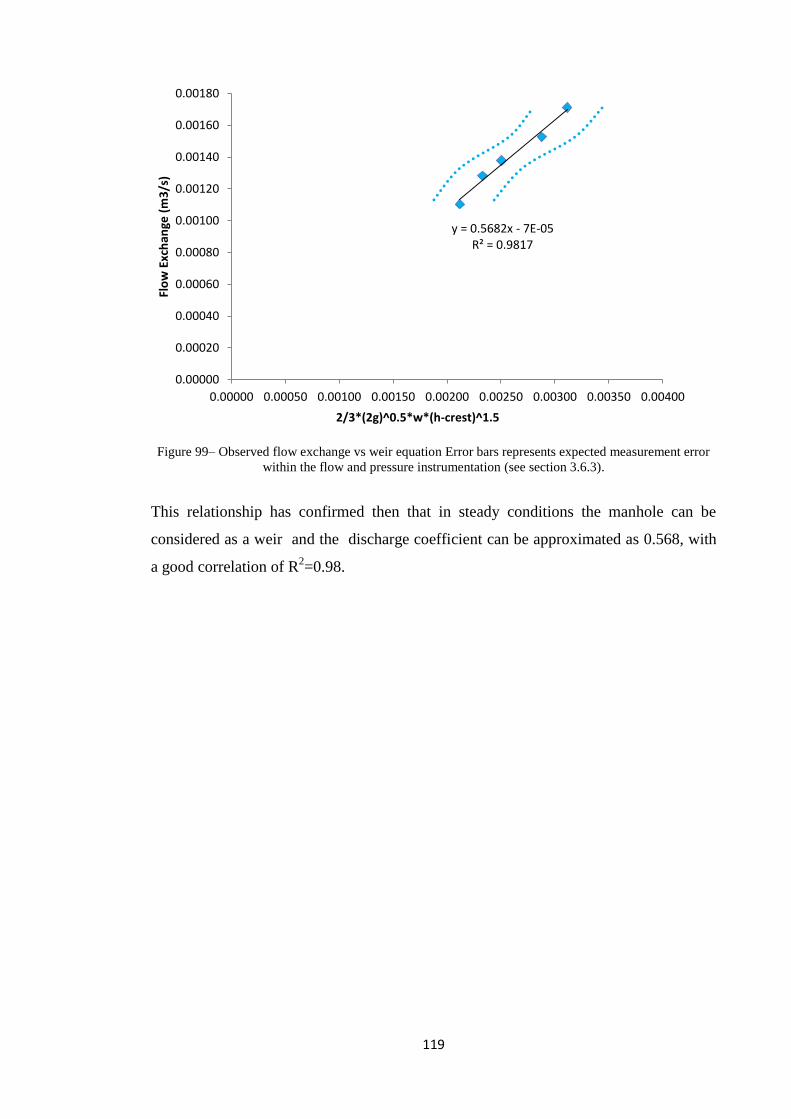
119
Figure 99– Observed flow exchange vs weir equation Error bars represents expected measurement error
within the flow and pressure instrumentation (see section 3.6.3).
This relationship has confirmed then that in steady conditions the manhole can be
considered as a weir and the discharge coefficient can be approximated as 0.568, with
a good correlation of R2=0.98.
y = 0.5682x - 7E-05 R² = 0.9817
0.00000
0.00020
0.00040
0.00060
0.00080
0.00100
0.00120
0.00140
0.00160
0.00180
0.00000 0.00050 0.00100 0.00150 0.00200 0.00250 0.00300 0.00350 0.00400
Flo
w E
xch
ange
(m
3/s
)
2/3*(2g)^0.5*w*(h-crest)^1.5
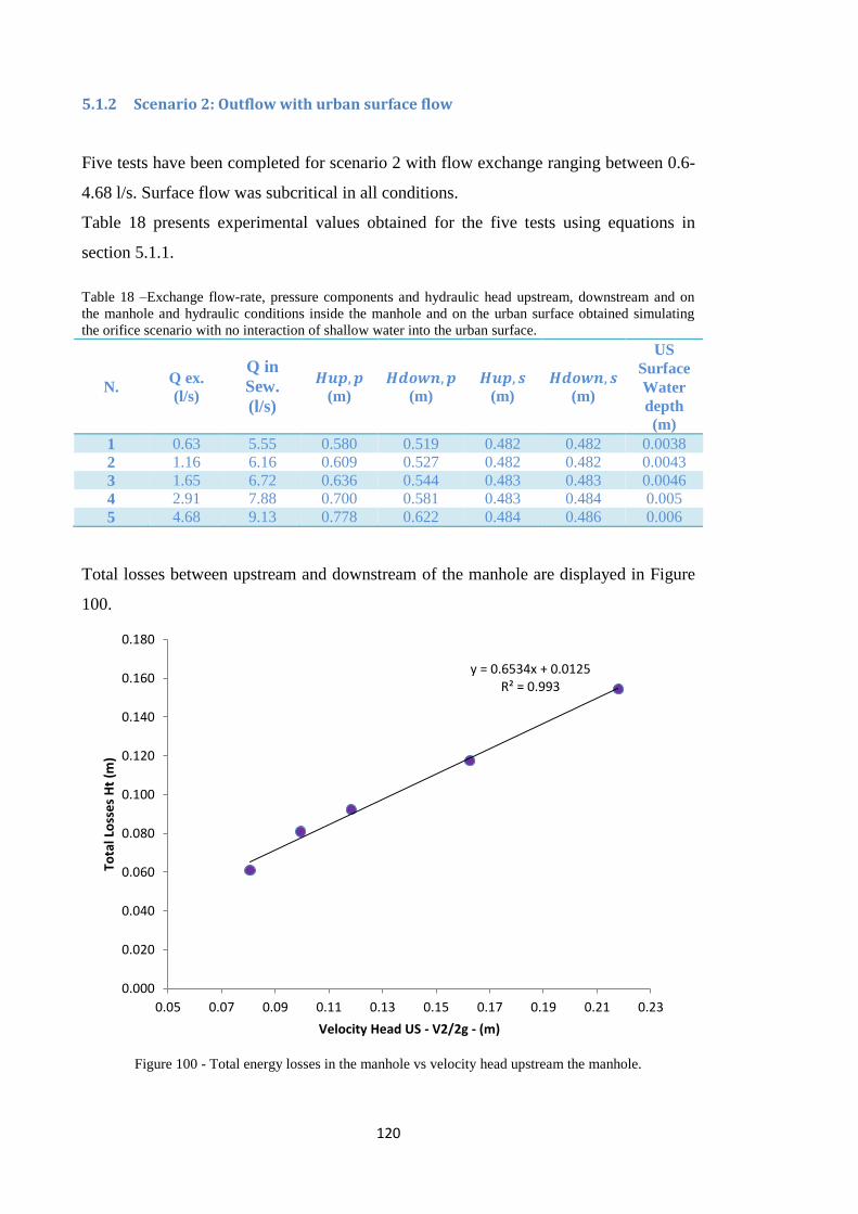
120
5.1.2 Scenario 2: Outflow with urban surface flow
Five tests have been completed for scenario 2 with flow exchange ranging between 0.6-
4.68 l/s. Surface flow was subcritical in all conditions.
Table 18 presents experimental values obtained for the five tests using equations in
section 5.1.1.
Table 18 –Exchange flow-rate, pressure components and hydraulic head upstream, downstream and on
the manhole and hydraulic conditions inside the manhole and on the urban surface obtained simulating
the orifice scenario with no interaction of shallow water into the urban surface.
N. Q ex.
(l/s)
Q in
Sew.
(l/s)
𝑯𝒖𝒑,𝒑
(m) 𝑯𝒅𝒐𝒘𝒏,𝒑
(m) 𝑯𝒖𝒑, 𝒔
(m) 𝑯𝒅𝒐𝒘𝒏, 𝒔
(m)
US
Surface
Water
depth
(m) 1 0.63 5.55 0.580 0.519 0.482 0.482 0.0038 2 1.16 6.16 0.609 0.527 0.482 0.482 0.0043 3 1.65 6.72 0.636 0.544 0.483 0.483 0.0046 4 2.91 7.88 0.700 0.581 0.483 0.484 0.005 5 4.68 9.13 0.778 0.622 0.484 0.486 0.006
Total losses between upstream and downstream of the manhole are displayed in Figure
100.
Figure 100 - Total energy losses in the manhole vs velocity head upstream the manhole.
y = 0.6534x + 0.0125 R² = 0.993
0.000
0.020
0.040
0.060
0.080
0.100
0.120
0.140
0.160
0.180
0.05 0.07 0.09 0.11 0.13 0.15 0.17 0.19 0.21 0.23
Tota
l Lo
sse
s H
t (m
)
Velocity Head US - V2/2g - (m)

121
A linear relationship exists between hydraulic head in the pipe and flow exchange. This
can be expressed in the form of the orifice equation (Figure 101).
Figure 101– Observed flow exchange vs orifice equation Error bars represents expected measurement
error within the flow and pressure instrumentation (see section 3.6.3).
This relationship has confirmed then that in steady conditions the manhole can be
considered as a orifice and the discharge coefficient can be approximated as 0.0883,
with a good correlation of R2=0.98.
y = 0.0883x - 0.0051 R² = 0.9849
0
0.001
0.002
0.003
0.004
0.005
0.006
0.05 0.06 0.07 0.08 0.09 0.1 0.11 0.12
Flo
w e
xch
ange
(m
3/s
)
A [2g(hu-hd)]0.5

122
5.1.3 Scenario 3: Outflow with interaction of shallow water in the urban surface
This final scenario replicates the water exceeding the manhole and reaching the urban
surface where there is also a component of shallow surface flow running from the inlet
tank to the outlet tank (Q2>0).
Figure 102- Examples of sewer to surface exchange simulated with the experimental facility.
The hydraulic parameters for each of the 6 tests are displayed in table 19.
Table 19 - Exchange flow-rate, pressure components and hydraulic head upstream, downstream and on
the manhole and hydraulic conditions inside the manhole and on the urban surface obtained simulating
the orifice scenario with interaction of shallow water into the urban surface.
Test
N.
Qex.
(l/s)
Q in
Sew.
(l/s)
𝑯𝒖𝒑,𝒑
(m) 𝑯𝒅𝒐𝒘𝒏,𝒑
(m) 𝑯𝒖𝒑, 𝒔
(m) 𝑯𝒅𝒐𝒘𝒏, 𝒔
(m)
US
Surface
Water
depth
(m)
Total
Head
Losses
Ht (m)
Rem
(/)
1 1.26 5.52 0.584 0.520 0.539 0.565 0.011 0.0376 93665 2 2.46 6.71 0.638 0.549 0.530 0.578 0.012 0.0399 113894 3 3.57 7.87 0.701 0.585 0.525 0.597 0.013 0.0441 133485 4 4.39 8.77 0.757 0.614 0.523 0.611 0.0135 0.0542 148810 5 5.05 9.43 0.799 0.637 0.521 0.625 0.014 0.0586 159924 6 5.51 9.90 0.833 0.654 0.521 0.638 0.0141 0.0618 167857
Where Rep= Reynolds through the pipe and Frs = Froude on urban surface.
Based on scaling factors, as discussed in section 3.1 the tests conducted here represent a
“full scale” flow velocity range of 0.21-0.38 m/s within the pipes and 0.19-0.25 m/s on
the urban surface. Figure 103 presents the relationship between the total energy losses
within the system and velocity head of the inlet flow.
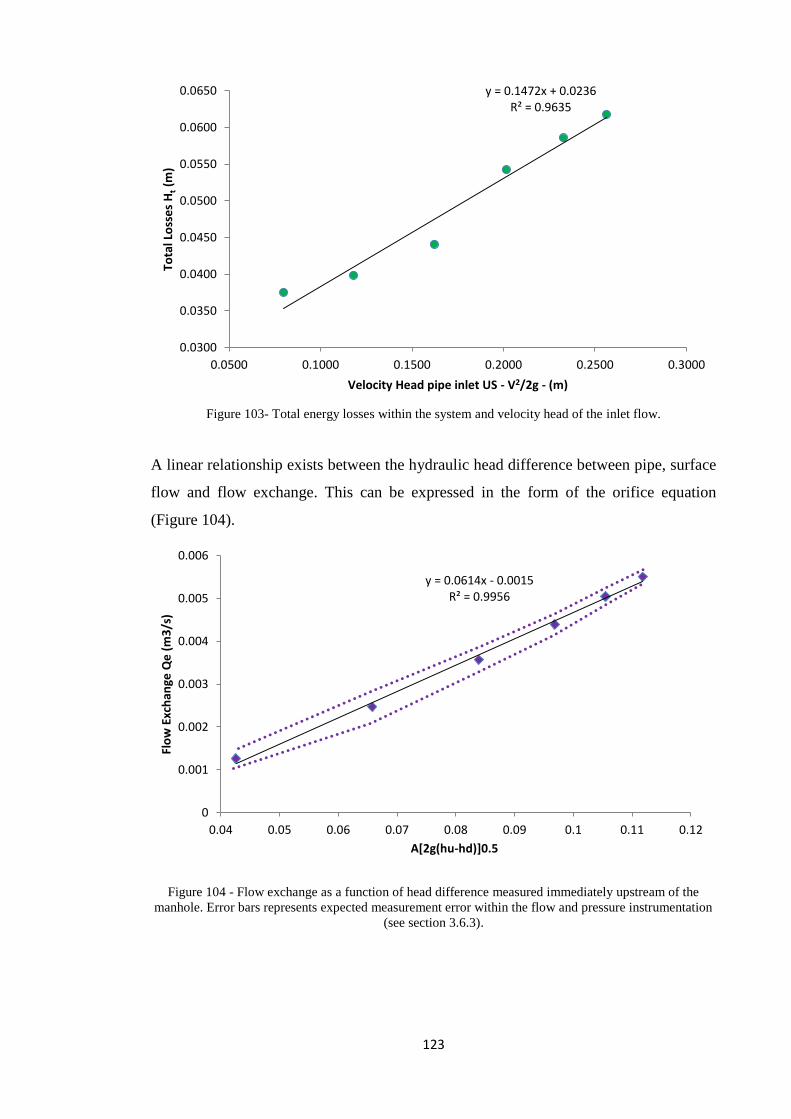
123
Figure 103- Total energy losses within the system and velocity head of the inlet flow.
A linear relationship exists between the hydraulic head difference between pipe, surface
flow and flow exchange. This can be expressed in the form of the orifice equation
(Figure 104).
Figure 104 - Flow exchange as a function of head difference measured immediately upstream of the
manhole. Error bars represents expected measurement error within the flow and pressure instrumentation
(see section 3.6.3).
y = 0.1472x + 0.0236 R² = 0.9635
0.0300
0.0350
0.0400
0.0450
0.0500
0.0550
0.0600
0.0650
0.0500 0.1000 0.1500 0.2000 0.2500 0.3000
Tota
l Lo
sse
s H
t (m
)
Velocity Head pipe inlet US - V2/2g - (m)
y = 0.0614x - 0.0015 R² = 0.9956
0
0.001
0.002
0.003
0.004
0.005
0.006
0.04 0.05 0.06 0.07 0.08 0.09 0.1 0.11 0.12
Flo
w E
xch
ange
Qe
(m
3/s
)
A[2g(hu-hd)]0.5

124
This relationship has confirmed then that in steady conditions the manhole can be
considered as a orifice and the discharge coefficient can be approximated as 0.061,
with a good correlation of R2=0.99.

125
6 Conclusions
The aim of this thesis was to use a physical model to improve understanding of flood
risk in the urban environment. Four specific research objectives were identified,
requiring two distinct physical model setups to be designed, constructed and tested. The
first experimental setup was based on an existing laboratory model at the University of
Sheffield, tests were conducted to identify local head losses through manholes under a
range of inlet conditions and flow rates, as well as test and verify the performance of
numerical models (SIPSON and SWMM) during scaled unsteady storm flow events.
This work required modification of the existing physical model inlet conditions in order
to achieve the flow rates and Reynolds numbers required. The main findings of this
phase of work are that the energy loss coefficient found for manholes with a “in line”
configuration fit within the range of existing values found in literature. The work has
presented new head loss values for manholes characterized by multiple inlets, with a
lateral inflow orientated at 45 degrees to the main flow direction. These are significantly
higher than those for in line manholes, this is most likely due to more complex flow
patterns which cause effects of acceleration and retardation and flow interference. K
values are sensitive to upstream and downstream pipe flow conditions. Kij values for
junction manholes have been compared to existing theoretical frameworks; however
differences in trends predicted using the frameworks and experimental observations are
observed. Overall hydraulic computer models replicating the physical system reproduce
the hydraulic characteristics well. Considering friction losses SIPSON is the model that
best reproduces the experimental data for manhole 1, 2, 3, 4, 5 of event 1 and 2
presented while SWMM better represents experimental data related to manhole 6
(downstream in the system) for both events. Tests have shown that by including local
head losses, SWMM improves its performance. The analysis has demonstrated that
neglecting local energy losses reduces their performance. This confirms the need to
provide more experimental data to improve the accuracy and efficiency of computer
models.
The second phase of the research involved the construction of a novel above/below
ground flow interaction model. This model was designed to provide datasets concerning
one of the most significant current uncertainties in urban flood modelling, regarding
energy losses and flow interaction at the interface between pipe network and surface

126
flow at manhole junctions. The aim of this phase of the research was to quantify the
suitability of weir and orifice equations to describe the interaction between above and
below ground system, and determine a suitable range of coefficients of these equations.
The main findings of this phase of the work were the confirmation that weir and orifice
equations can be used to quantify flow exchange between a sewer system linked to an
urban surface through a single manhole under steady flow conditions. This has been
verified under different pluvial conditions replicated within the facility. Additionally,
for each specific scenario a range of discharge coefficients has been calculated. For a
typical weir scenario, with water running onto the urban surface reaching the sewer
system, 0.57 is the best fit value. Regarding the orifice scenario, for simulations that
have been characterized by water escaping the manhole reaching the urban surface the
best fit coefficient is 0.0883. Finally, when there is a complex interaction between water
running into the surface and water escaping the sewer from the manhole the best fit
discharge coefficient is 0.061.
The experimentally derived discharge coefficient in the orifice flow regime was unable
to be directly compared to other studies due to the lack of Co prediction at low head in
the available literature and similar experimental studies completed.
The limitations of the present study should be noted. The current model considers an
open manhole which discharges directly into the surface; this does not include the
effects of any manhole lid on the flow interaction. In addition, unsteady events have not
yet been considered, further research should consider how energy losses are effected by
rapidly changing flow rates which are common in urban flooding situations.

127
7 Further work
This model considers an open manhole which discharges directly into the surface.
Despite the fact that in some countries this aspect is something normal during urban
flooding events (in Portugal for example the Civil Protection has to remove all the gates
to avoid blockages as showed in figure 105a and 105b), manholes are covered by
gridlines which influence the discharge of the flow.
Figure 105– a) Viana do Castelo, urban inundation (Source ARMENIO BELO/LUSA, accessed the
06/06/2014 http://www.tvi24.iol.pt/sociedade/mau-tempo-lisboa-cheias-inundacoes-meteorologia-
tvi24/1203790-4071.html) b) Another example, urban inundation and gate removal. (Photo LUIS
PARDAL/GLOBAL IMAGENS, accessed the 06/06/2014
(Right)http://www.jn.pt/PaginaInicial/Sociedade/Interior.aspx?content_id=2862575)
Hence future work will focus on designing a “lid” above the manhole to make the
system more realistic and provide more datasets with different configurations.
As described, computer models are inherently problematic to verify due to the
difficultly of acquiring reliable data during the flood event and most models are
calibrated using only an estimated measure of the extent of flooding. Similarly, existing
models do not currently attempt to quantify the transport and fate of sewer derived
pollutants and hence it is difficult to assess the risk of exposure and the potential impact
of flood waters on health. Manholes are interaction points where there is a critical
transfer of flow and pollution and this process is difficult to quantify due to the complex
and time varying nature. Understanding such behaviour is essential to accurately
evaluate urban flood risk by hydraulic models.
Modelling the transport of harmful contaminants/pollutants from sewer interface points
is a relevant step to increase the accuracy of computer models and it has only recently
been attempted (Pathirana, 2011). Coupled with studies of health risk from exposure to
flood water (Fewtrell et al, 2011) such models could be used to predict both areas most
at risk from contamination and the potential health impacts of flood events. The large
128
number of uncertainties involved (e.g. impact of urban topographies on hydraulic
profiles, storage zones and dispersion) means that such modelling is at an early stage,
and is extremely prone to inexact calibration and verification.
The next feasible outputs from this experimental facility will provide the first data sets
for such advanced calibration and verification, thereby providing enhanced
opportunities for the prediction of accurate combination between flood flow and
contaminant movement during flood events. The results will subsequently be used to
improve the accuracy of commercial modelling software with significant benefits in the
evaluation of flood risk and the prioritisation of asset investment.
Future work will utilise this unique surface/subsurface together with numerical and
computational advances in the solution of the hydraulic and pollutant transport
equations. The main challenge will consider the experimentally investigation of the
transport of soluble material from sewers to surface flows via manholes and determine
the transport and mixing characteristics in typical overland shallow flow flooding
conditions.
Pollutant transport through the system will be quantified in both steady and time
varying flow conditions. In time varying tests, dye will be injected into the pipe
immediately prior to a manhole surcharge event to simulate contaminates being flushed
through the system and quantify the total transfer of mass to surface flow via an
individual manhole. Different surface topographical setups (Figure 106) will be tested
to determine how features influence mass transport in surface flow via the creation of
turbulent structures, local velocity shear and trapping zones (characterised with PIV
measurements, using the equipment designed and tested during the final part of this
research). Three test surface topographies will be installed and tested which are
designed to simulate the effect of typical street features. The geometry of surface
features will be based on the sewer scaling.
1. Featureless bed – Initial tests to characterise mixing over a range of flow conditions.
2. Road and pavement – At low flows, pavements will promote transverse velocity
gradients and shear. At higher flows, flow will overtop pavements, potentially
creating turbulent mixing layers and considerable extra velocity shear.

129
3. Trapping zones - A range of street features may act as trapping zones and affect the
transport of pollutants. Such zones will be simulated by constructing gaps in the
pavement profile.
Dimensionless mixing coefficients (i.e. normalised by flow depths and shear velocities)
within the surface flow will be determined. Characterisation of the velocity fields via
PIV developed during this research will be determined. Mixing coefficients will be
initially quantified for the featureless bed in steady uniform flow conditions via both
analytical and numerical solutions. By achieving that, a unique data set that will be
made available to other researchers and software developers.
Once these results will be provided, considering that hydraulic models are increasingly
being used to plan significant asset investment and form the basis of flood
awareness/warning schemes, there will be significant benefits in terms of more efficient
drainage design/investment and increased resilience to flood events.
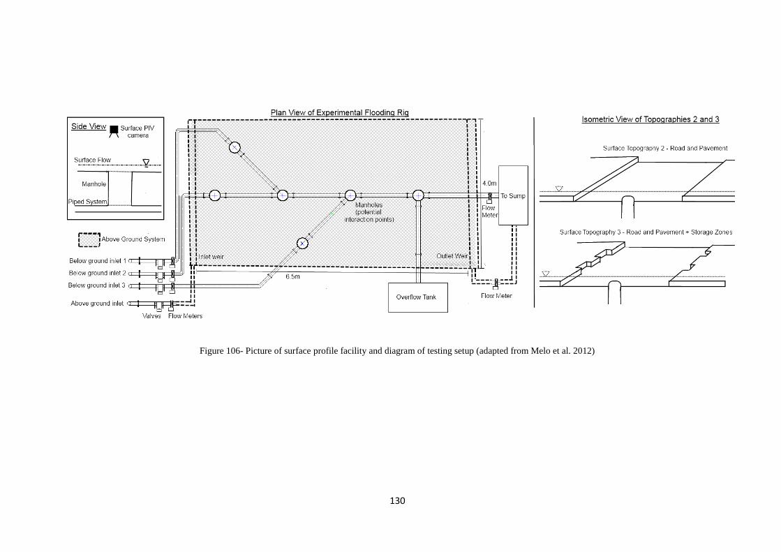
130
Figure 106- Picture of surface profile facility and diagram of testing setup (adapted from Melo et al. 2012)

131
8 References
Ackers P. (1959) An investigation of head losses at sewer manholes. Civil Engineering
and Public Work Review, 54, 637, 882-884 and 1033-1036.
Archer B., Bettes F., Colyer P.J. (1978) Head losses and air entrainment at surcharged
manholes. Report No IT 185, Hydraulic Research Station, Wallingford, England.
Arao, S., Kusuda T., Moriyama K., Hiratsuka S., Asada J., Hirose N. (2012) Energy
losses at three-way circular drop manholes under surcharged conditions. Water
Science and Technology, 66, 1.
Ashley, R.M., Balmforth, D.J., Saul, A.J., Blanskby, J.D. (2005) Flooding in the future -
Predicting climate change, risks and responses in urban areas. Water Science and
Technology, 52, 5, 265-273.
Asztely M. (1995) Literature Review of energy losses in manholes. The Universiy of
Goteborg, Department of Hydraulics.
Bamford T.B., Digman C.J., Balmforth D.J., Waller S., Hunter N. (2008) Modelling
flood risk – an evaluation of different methods. WaPUG Autumn Conference,
Blackpool.
Bazin P.H., Nakagawa H., Kawaike K., paquier A., Mignot E. (2014) Modeling Flow
Exchanges between a Street and an Underground Drainage Pipe during Urban
Floods. Journal of Hydraulic Engineering, 140, 10.
Biron P., Best J.L., Roy A.G. (1996) Effects of bed discordance on flow dynamics at
open channel confluences. Journal of Hydraulic Engineering, 122, 12, 676-682.
Carpenter G. & Company, LLC, Guy Carpenter & Company Ltd. or Guy Carpenter &
Company, S.A.S. (2013) Floods in Eastern Australia.
Chanson Hubert, (1999) Hydraulics of Open Channel Flow: An Introduction - Basic
principles, Sediment Motion, Hydraulic Modeling, Design of Hydraulic Structures,
Elsevier.
Chen A., Djordjievic S., Leandro J., Savic D. (2007) The urban inundation model with
bidirectional flow interaction between 2D overland surface and 1D sewer networks.
Workshop, Novatech 2007, 25-28 June, Lyon, France.
City and County of San Francisco 2030 Sewer System Master Plan (2011) Task 500,
Technical Memorandum No.506, Collection System Rehabilitation Program. Climate
Change Report.

132
Cohen B., (2006) Urbanization in developing countries: Current trends, future
projections, and key challenges for sustainability. Technology in Society, 28, 63–80.
Defra. The appraisal of human related intangible impacts of flooding. Defra, Flood
management division, R&D Technical Report FD2005/TR, London, UK. 2004.
Del Giudice G., Gisonni C. and Hager W. H. (2000). Supercritical flow in bend
manhole. Journal of Irrigation and Drainage Engineering, 126, 48-56.
Del Giudice G., Hager W.H. (2001) Supercritical flow in bend manhole. Journal of
Irrigation and Drainage Engineering, ASCE, 126, 1, 48-56.
Djordjevic S., Prodanovic D., Maksimovic C. (1999) An approach to simulation of dual
drainage, Water Science and Technology, 39, 9, 95-103.
Djordjevic S., Prodanovic D., Maksimovic C., Ivetic M. and Savic D. (2005). SIPSON -
simulation of interaction between pipe flow and surface overland flow in networks.
Water Science and Technology, 52, 5, 275-283.
Djordjevic S., Saul A.J., Tabor G.R., Blanksby J., Galambos I, Sabtu N. and Sailor G.
(2013). Experimental and numerical investigation of interactions between above and
below ground drainage systems. Water Science and Technology, Vol. 67, 3, 535-42.
Dottori F., Todini E. (2013) Testing a simple 2D hydraulic model in an urban flood
experiment. Hydrological Processes, 27, 9, 1301-1320.
Environment Agency (2010) The costs of the 2007 summer floods in England.
Environmental Engineering Dictionary, Mehdi Ahmadi,
http://www.ecologydictionary.org/URBAN_FLOODING (accessed the 06/06/2014).
Fewtrell L. & Kay D. An attempt to quantify the health impacts of flooding in the UK
using an urban case study. Public Health 2008, 122, 446–451.
Fewtrell L., Kay D., Watkins J., Davies C., Francis C. (2011) Journal of Flood Risk
Management, 4, Issue 2, 77-87.
Flood Risk in Brazil, http://www.preventionweb.net/files/20634_floodriskinbrazil1.pdf ,
(Accessed on the 4th
of November 2013).
Gargano R., Hager W.H. (2002) Supercritical across sewer manholes. Journal of
Hydraulic Engineering, ASCE, 128, 11, 1014-1017.
Gisonni C, Hager W.H. (2002) Supercritical flow in the junction. Journal of Irrigation
and Drainage Engineering, 126, 1, 48-56.
Gurram S.K., Karki K.S. (2000) Subcritical open-channel junction flow. Journal of
Hydraulic Engineering, ASCE, 126, 1, 87-91.

133
Hager W.H. (1989) Transitional flow in channel junctions. Journal of Hydraulic
Engineering, ASCE, 115, 2, 243-259.
Hare C.M. (1983) Magnitude of hydraulic losses at junctions in piped drainage systems.
Civil engineering transactions, Institute of Civil Engineers, 71-77.
Howarth D.A., Saul A.J. (1984) Energy loss coefficient at manholes. Proceedings of the
3rd
International Conference on Urban Storm Drainage, June 4-8, 127-136,
Gothenburg, Sweden.
Hsu C.C., Wu F.S., Lee W.J. (1998) Flow at equal width open channel junction. Journal
of Hydraulic Engineering, ASCE, 124, 2, 186-191.
Hunter, N. M., Bates, P. D., Neelz, S., Pender, G., Villanueva, I., Wright, N. G., Liang,
D., Falconer, R. A., Lin, B., Waller, S., Crossley, A. J. & Mason, D. C. (2008)
Benchmarking 2D hydraulic models for urban flooding. Water Management, 161
(WM1), 13–30.
Hunter NM, Bates PD, Horritt MS, Wilson MD. (2007). Simple spatially distributed
models for predicting flood inundation: a review. Geomorphology 90: 208–225.
IPCC (2014) Summary for policymakers. Climate Change 2014: Impacts, Adaptation
and Vulnerability.
Jha A.K., Bloch R., Lamond J. (2012) Cities and Flooding. A guide to integrated urban
flood risk management for the 21st century. © 2012 International Bank for
Reconstruction and Development/ International Development Association.
Johnston A.J., Volker R.E. (1990) Head losses at junction boxes. Journal of Hydraulic
Engineering, 116, 326-341.
Kerr Wood Leidal Associates LTD, Consulting Engineers (2008). Vulnerability of
Vancouver Sewerage Area Infrastructure to Climate Change, Final Report. METRO
Vancouver, KWL File No. 251.219.
Liebmann H (1970) Der Einfluss von Einsteigschachten auf den Abflussvorgang in
Abwasserkanalen. Wasser und Abwasser in Forschung und Praxis. Erich Schmidt
Verlag (in German).
Lindvall G. (1984) Head losses at surcharged manholes with a main pipe and a 90
degrees lateral. Proceedings of the 3rd
International Conference on Urban Storm
Drainage, June 4-8, 137-146, Gothenburg, Sweden.
Lindvall G. (1987) Head losses at surcharged manholes. Proceedings of the AIRH- XXII
congress – IAHR and the Fourth International Conference on Urban Storm Drainage,
140-141, Lausanne, Switzerland.

134
Lopes P. , Lenadro J., Carvalho R.F., Pascoa P., Martins R. (2013). Numerical and
experimental investigation of a gully under surcharge conditions. Urban Water
Journal, 10.1080/1573062X.2013.831916.
Mark O. (1989) En matematisk model for energitab I broØnde. Thesis presented at the
Institute of Hydrodynamics and Hydraulic Engineering, Technical University of
Denmark. Lyngby, Denmark, in partial fulfilment of the requirements for the degree
of Master Science.
Mark O., Weesakul S., Apirumanekul C., Boonya Aronnet S., Djordjevic S. (2004)
Potential and limitations of 1D modeling of urban flooding. Journal of Hydrology,
299, 284-299.
Marsalek J. (1981) Energy losses at straight-flow through sewer junctions. Research
report No 111. Research program for the abatement of municipal pollution under
provisions of the Canada-Ontario agreement on the Great Lakes Water Quality.
Training and Technology Transfer Division, Environmental Protection Service,
Environment Canada, Ottawa, Ontario, KIA, 1C8.
Marsalek J., (1984) Head losses at sewer junction manholes. Journal of Hydraulics
Engineering, ASCE, 110, 8, 1150–1154.
Marsalek J., (1985) Head losses at selected sewer manholes. Unpublished report,
National Water Research Institute, Burlington, Ontario.
Marsalek J. (1987) Head losses at junction of two opposing lateral sewers. Proceedings
of the AIRH- XXII congress – IAHR and the Fourth International Conference on
Urban Storm Drainage, 140-141, Lausanne, Switzerland.
Marsalek, J., and Greck, B. J. (1988) Head losses at manholes at 90°bend. Canadian
Journal of Civil Engineering, 15, 851–858.
Massey B.S., Ward Smith J. (1998) Mechanics of Fluids, Seventh Edition, Volume 1.
Melo N., Leandro J., Shucksmith J., Rubinato M., Djordjevic S., Saul A.J., Ramos H.,
L.M.P.de Lima J. (2012) Modelling Internal Boundary Conditions of a Sewer
Network. 9th
International Conference on Urban Drainage Modelling, Belgrade,
Serbia.
Met Office report, Missler C., Eastman M.D. The Creator Beyond Time and Space. The
Word for Today, 12-17.
Mrowiec M. (2007) Head Loss at two-way circular manholes in drainage systems under
surcharge conditions. Environment Protection Engineering, 33, 2.

135
Mugdal B., Pani B.S. (1993) Head Losses in sewer manholes. Proceedings of the Sixth
International Conference on Urban Storm Drainage, Niagara Falls, Ontario, Canada,
134-139.
Neal J.C., Bates P.D., Fewtrell T.J., Hunter N.M., Wilson M.D., Horritt M.S. (2009)
Distributed whole city water level measurements from the Carlisle 2005 urban flood
event and comparison with hydraulic model simulations. Journal of Hydrology, 368,
1-4, 42-55.
Notaro V., Fontanazza C.M., Freni G., La Loggia G. (2010). Uncertainty connected
with design rainfall for urban flood risk evaluation. Novatech, Lyon, France.
Ohl C. & Tapsell S. Flooding and human health. Br Med J 2000, 321, 1167–1168.
Phang X., O’Loughlin G. (2011) Pressure change at stormwater pits with part full flows.
12th
International Conference on Urban Drainage, Porto Alegre, Brazil, 10-15
September.
Parkin G. (2010) The September 2008 Morpeth flood: information gathering for
dynamic flood reconstruction. Summary Report 31 May 2010.
Pathirana A., Mahen D., Brdjanovic D. 12th
International Conference on Urban
Drainage Modelling, Porto Alegre, Brazil, September 2011.
Pedersen F.B. and Mark O. (1990) Head losses in storm sewer manholes: submerged jet
theory. Journal of Hydraulic Engineering, ASCE, 116, 11, 1317-1328.
Pfister M., Ginsonni C. (2014) Head Losses in Junction Manholes for free Surface
Flows in circular Conduits. Technical Note, Journal of Jydraulic Engineering, 140,
9.
Photo Another example, urban inundation and gate removal. (Photo LUIS
PARDAL/GLOBAL IMAGENS, accessed the 06/06/2014
http://www.jn.pt/PaginaInicial/Sociedade/Interior.aspx?content_id=2862575)
Photo Viana do Castelo, urban inundation (Source ARMENIO BELO/LUSA, accessed
the 06/06/2014 http://www.tvi24.iol.pt/sociedade/mau-tempo-lisboa-cheias-
inundacoes-meteorologia-tvi24/1203790-4071.html)
Prodanović D., Djordjević S., Maksimović Č. (1998) GIS assisted model for dual
drainage simulation. Hydroinformatics, ’98, 1, V.Babovic and L.C. Larsen (Eds).
Balkema, Rotterdam, 535-542.
Ramamurthy A.S., Zhu W. (1997) Combining flows in 90 º junctions of rectangular
closed conduits. Journal of Hydraulic Engineering, 123, 1012-1019.

136
Rouse, H., (1950) Engineering Hydraulics. Proceedings of the Fourth Hydraulics
Conference, Iowa Institute of Hydraulic Research, John Wiley and Sons, Inc., New
York.
Saldarriaga J., Bermúdez N., Rubio D.P. (2012) Hydraulic behaviour of junction
manholes under supercritical flow conditions, Journal of Hydraulic Research, 50, 6,
631-636.
Sangster W.M., Wood H.W., Smerdon E.T., Bossy H.S., (1958) Pressure changes at
storm drain junctions. Bulletin No. 41, Engineering Experiment Station, University
of Missouri.
Schmidt R. (2011) Urban Flood Risk in Dakar, Senegal. The World Bank, Africa
Disaster Risk Management.
Serre M., Odgaard A.J., Elder R.A. (1994) Energy loss at combining pipe junction.
Journal of Hydraulic Engineering, 120, 7, 808-830.
Seyoum S., Vojinovic Z., Price K.R., Weesakul S. (2012) Coupled 1D and Noninertia
2D flood inundation model for simulation of urban flooding. Journal of Hydraulic
Engineering, 138, 23-34.
Singh R., Social Vulnerability and Wastewater Related Risks: A case Study of Delhi.
Project “Vulnerability in Mega Cities: New approaches to analyse urban water
system in Delhi”.
Stovin V., Bennett P., Guymer I. (2013) Absence of a hydraulic threshold in small-
diameter surcharged manholes. Journal of Hydraulic Engineering, 139, 9, 984-994.
Taylor E.H. (1944) Flow characteristics at rectangular open channel junctions. Trans.
ASCE, 109, 893-912.
ten Veldhuis J.A.E. (2011) How the choice of flood damage metrics influences urban
flood risk assessment. Journal of Flood Risk Management, 4, Issue 4.
The Pitt Review (2008) An Update of the Foresight Future Flooding 2004 qualitative
risk analysis.
Tominaga A. (2007) Lesson learned from Tokai heavy rainfall. Journal of Disaster
Research, 2, No.1.
United Nations, Department of Economic and Social Affairs, Population Division:
World Urbanization Prospects, the 2011 Revision. New York, 2012.
Unwin D.M. (2008) Development of control algorithms: to describe flow discharge
reduction and energy loss at a manhole junction. Thesis (Ph.D.) - University of
Sheffield, Department of Civil and Structural Engineering.
137
Wang K. H., Cleveland T. G., Towsley C. and Umrigar D. (1998) Head loss at
manholes in surcharged sewer systems. Journal of the American Water Resources
Association, 34, 6, 1391-1400.
WaPUG. Code of practice for the hydraulic modelling of sewer systems. 2002.
Available from: http://www.ciwem.org/media/44426/Modelling_COP_Ver_03.pdf.
(Accessed 16th
August 2011).
Water and wastewater services in Columbo to be improved with ABD funding.
(Accessed on 06/06/2014, http://www.waterworld.com/articles/2012/10/water-and-
wastewater-services-in-columbo-restored-by-adb-300m-funding.html).
Weitbrecht V., Jirka G.H. (2001) Flow patterns and exchange processes in dead zones
rivers. Proceedings of the IAHR Congress 2001, Beijing.
Weitbrecht V., Kuhn G., Jirka G.H. (2002) Large scale PIV-measurements at the
surface of shallow water flows. Journal of Flow Measurement and Instrumentation,
13, 237-245.
WRc, 1987. A Guide to Short-Term Flow Surveys of Sewer Systems. Swindon: Water
Research Centre.
Wu, S. and Rajaratnam, N. (1996). Submerged Flow Regimes of Rectangular Sharp-
Crested Weirs. Journal of Hydraulic Engineering, 122, 7, 412–414.
Yevjevich V., Barnes A.H., (1970) Flood routing through storm drains. Part 1-4,
Hydrology Papers 43-46, Colorado State University, Fort Collins, Colorado, USA.
Young P.C., Jakeman A.J., McMurtrie R. (1980) An instrumental variable method for
model order identification. Automatica, 16, 281-294.
Zhao C.H., Zhu D. Z., Rajaratnam N. (2004) Supercritical sewer flows at combining
junction: a case study of Edworthy Trunk Junction, Calgary, Alberta. Journal of
Environmental Engineering Science, NRC, 3, 5, 343-353.
Zhao C.H., Zhu D. Z., Rajaratnam N. (2006) “Experimental Study of Surcharged Flow
at Combining Sewer Junctions”. Journal of Hydraulic Engineering, 132, 12, 1259-
1271.
Zhao C.H., Zhu D. Z., Rajaratnam N. (2008) “Computational and Experimental Study
of Surcharged Flow at a 90° Combining Sewer Junction”. Journal of Hydraulic
Engineering, 134(6), 688–700.
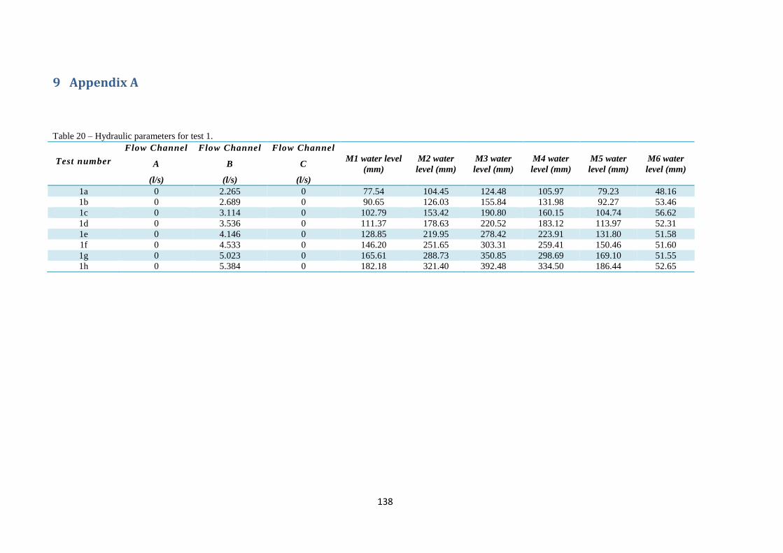
138
9 Appendix A
Table 20 – Hydraulic parameters for test 1.
Test number
Flow Channel
A
(l/s)
Flow Channel
B
(l/s)
Flow Channel
C
(l/s)
M1 water level
(mm)
M2 water
level (mm)
M3 water
level (mm)
M4 water
level (mm)
M5 water
level (mm)
M6 water
level (mm)
1a 0 2.265 0 77.54 104.45 124.48 105.97 79.23 48.16
1b 0 2.689 0 90.65 126.03 155.84 131.98 92.27 53.46
1c 0 3.114 0 102.79 153.42 190.80 160.15 104.74 56.62
1d 0 3.536 0 111.37 178.63 220.52 183.12 113.97 52.31
1e 0 4.146 0 128.85 219.95 278.42 223.91 131.80 51.58
1f 0 4.533 0 146.20 251.65 303.31 259.41 150.46 51.60
1g 0 5.023 0 165.61 288.73 350.85 298.69 169.10 51.55
1h 0 5.384 0 182.18 321.40 392.48 334.50 186.44 52.65
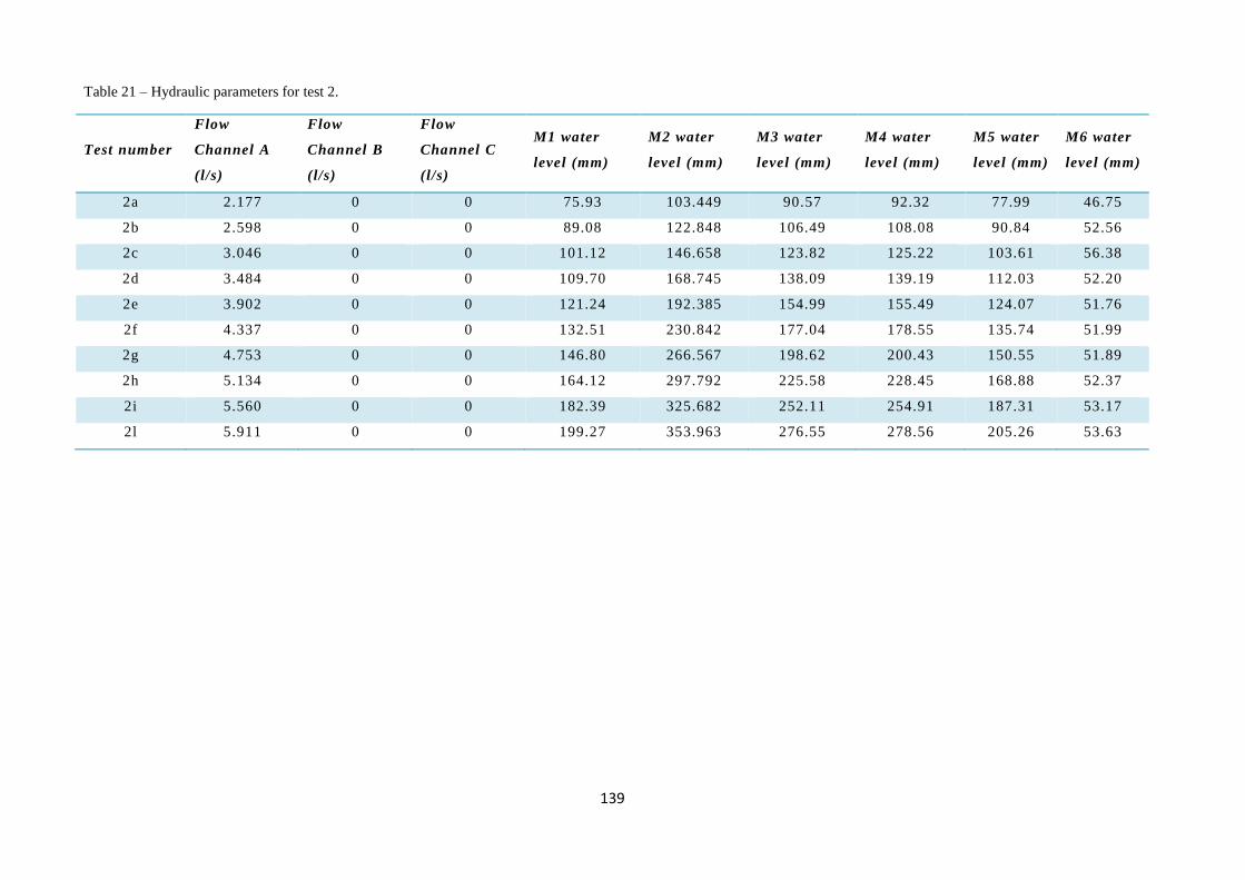
139
Table 21 – Hydraulic parameters for test 2.
Test number
Flow
Channel A
(l/s)
Flow
Channel B
(l/s)
Flow
Channel C
(l/s)
M1 water
level (mm)
M2 water
level (mm)
M3 water
level (mm)
M4 water
level (mm)
M5 water
level (mm)
M6 water
level (mm)
2a 2.177 0 0 75.93 103.449 90.57 92.32 77.99 46.75
2b 2.598 0 0 89.08 122.848 106.49 108.08 90.84 52.56
2c 3.046 0 0 101.12 146.658 123.82 125.22 103.61 56.38
2d 3.484 0 0 109.70 168.745 138.09 139.19 112.03 52.20
2e 3.902 0 0 121.24 192.385 154.99 155.49 124.07 51.76
2f 4.337 0 0 132.51 230.842 177.04 178.55 135.74 51.99
2g 4.753 0 0 146.80 266.567 198.62 200.43 150.55 51.89
2h 5.134 0 0 164.12 297.792 225.58 228.45 168.88 52.37
2i 5.560 0 0 182.39 325.682 252.11 254.91 187.31 53.17
2l 5.911 0 0 199.27 353.963 276.55 278.56 205.26 53.63
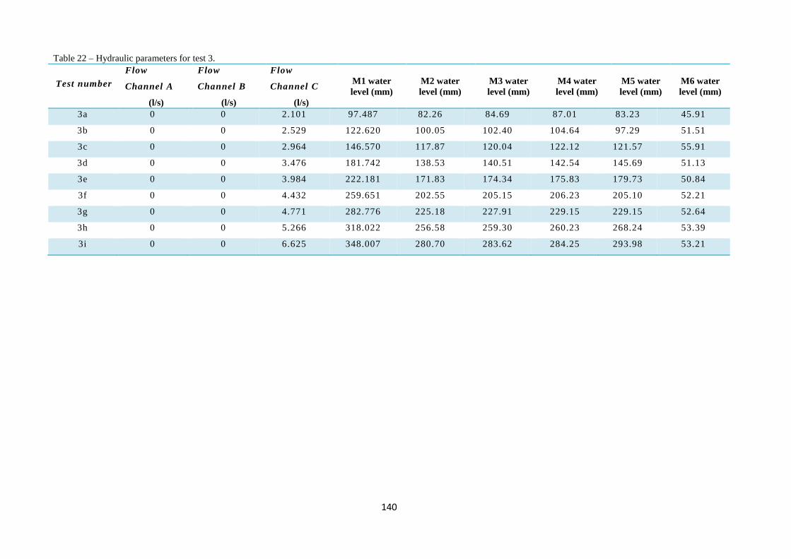
140
Table 22 – Hydraulic parameters for test 3.
Test number
Flow
Channel A
(l/s)
Flow
Channel B
(l/s)
Flow
Channel C
(l/s)
M1 water
level (mm) M2 water
level (mm) M3 water
level (mm) M4 water
level (mm) M5 water
level (mm)
M6 water
level (mm)
3a 0 0 2.101 97.487 82.26 84.69 87.01 83.23 45.91
3b 0 0 2.529 122.620 100.05 102.40 104.64 97.29 51.51
3c 0 0 2.964 146.570 117.87 120.04 122.12 121.57 55.91
3d 0 0 3.476 181.742 138.53 140.51 142.54 145.69 51.13
3e 0 0 3.984 222.181 171.83 174.34 175.83 179.73 50.84
3f 0 0 4.432 259.651 202.55 205.15 206.23 205.10 52.21
3g 0 0 4.771 282.776 225.18 227.91 229.15 229.15 52.64
3h 0 0 5.266 318.022 256.58 259.30 260.23 268.24 53.39
3i 0 0 6.625 348.007 280.70 283.62 284.25 293.98 53.21
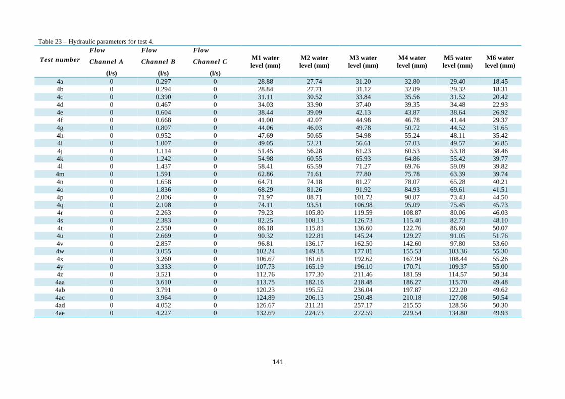
141
Table 23 – Hydraulic parameters for test 4.
Test number
Flow
Channel A
(l/s)
Flow
Channel B
(l/s)
Flow
Channel C
(l/s)
M1 water
level (mm) M2 water
level (mm) M3 water
level (mm) M4 water
level (mm) M5 water
level (mm)
M6 water
level (mm)
4a 0 0.297 0 28.88 27.74 31.20 32.80 29.40 18.45
4b 0 0.294 0 28.84 27.71 31.12 32.89 29.32 18.31
4c 0 0.390 0 31.11 30.52 33.84 35.56 31.52 20.42
4d 0 0.467 0 34.03 33.90 37.40 39.35 34.48 22.93
4e 0 0.604 0 38.44 39.09 42.13 43.87 38.64 26.92
4f 0 0.668 0 41.00 42.07 44.98 46.78 41.44 29.37
4g 0 0.807 0 44.06 46.03 49.78 50.72 44.52 31.65
4h 0 0.952 0 47.69 50.65 54.98 55.24 48.11 35.42
4i 0 1.007 0 49.05 52.21 56.61 57.03 49.57 36.85
4j 0 1.114 0 51.45 56.28 61.23 60.53 53.18 38.46
4k 0 1.242 0 54.98 60.55 65.93 64.86 55.42 39.77
4l 0 1.437 0 58.41 65.59 71.27 69.76 59.09 39.82
4m 0 1.591 0 62.86 71.61 77.80 75.78 63.39 39.74
4n 0 1.658 0 64.71 74.18 81.27 78.07 65.28 40.21
4o 0 1.836 0 68.29 81.26 91.92 84.93 69.61 41.51
4p 0 2.006 0 71.97 88.71 101.72 90.87 73.43 44.50
4q 0 2.108 0 74.11 93.51 106.98 95.09 75.45 45.73
4r 0 2.263 0 79.23 105.80 119.59 108.87 80.06 46.03
4s 0 2.383 0 82.25 108.13 126.73 115.40 82.73 48.10
4t 0 2.550 0 86.18 115.81 136.60 122.76 86.60 50.07
4u 0 2.669 0 90.32 122.81 145.24 129.27 91.05 51.76
4v 0 2.857 0 96.81 136.17 162.50 142.60 97.80 53.60
4w 0 3.055 0 102.24 149.18 177.81 155.53 103.36 55.30
4x 0 3.260 0 106.67 161.61 192.62 167.94 108.44 55.26
4y 0 3.333 0 107.73 165.19 196.10 170.71 109.37 55.00
4z 0 3.521 0 112.76 177.30 211.46 181.59 114.57 50.34
4aa 0 3.610 0 113.75 182.16 218.48 186.27 115.70 49.48
4ab 0 3.791 0 120.23 195.52 236.04 197.87 122.20 49.62
4ac 0 3.964 0 124.89 206.13 250.48 210.18 127.08 50.54
4ad 0 4.052 0 126.67 211.21 257.17 215.55 128.56 50.30
4ae 0 4.227 0 132.69 224.73 272.59 229.54 134.80 49.93

142
4af 0 4.317 0 137.72 234.49 283.66 239.65 140.14 49.70
4ag 0 4.485 0 143.95 246.25 295.95 251.53 146.36 49.67
4ah 0 4.565 0 147.85 253.24 301.39 260.70 150.55 49.48
4ai 0 4.713 0 153.98 264.28 310.50 273.93 156.82 49.37
4aj 0 4.901 0 161.38 278.62 326.64 290.21 164.03 49.77
4ak 0 5.078 0 168.40 292.69 343.90 304.47 170.65 50.48
4al 0 5.171 0 172.24 299.84 353.55 312.51 174.21 50.64
4am 0 5.310 0 178.79 313.21 370.45 327.12 182.23 51.18
4an 0 5.418 0 184.34 323.84 382.84 339.55 187.96 51.50
4ao 0 5.556 0 193.88 338.08 400.26 355.08 196.56 51.32
4ap 0 5.711 0 202.67 354.26 420.26 373.96 205.25 51.47
4aq 0 5.802 0 207.75 363.94 432.04 381.97 210.00 51.68
4ar 0 5.943 0 212.97 375.05 445.27 393.34 215.32 51.40
4as 0 6.072 0 218.57 388.03 461.59 409.57 220.75 51.37
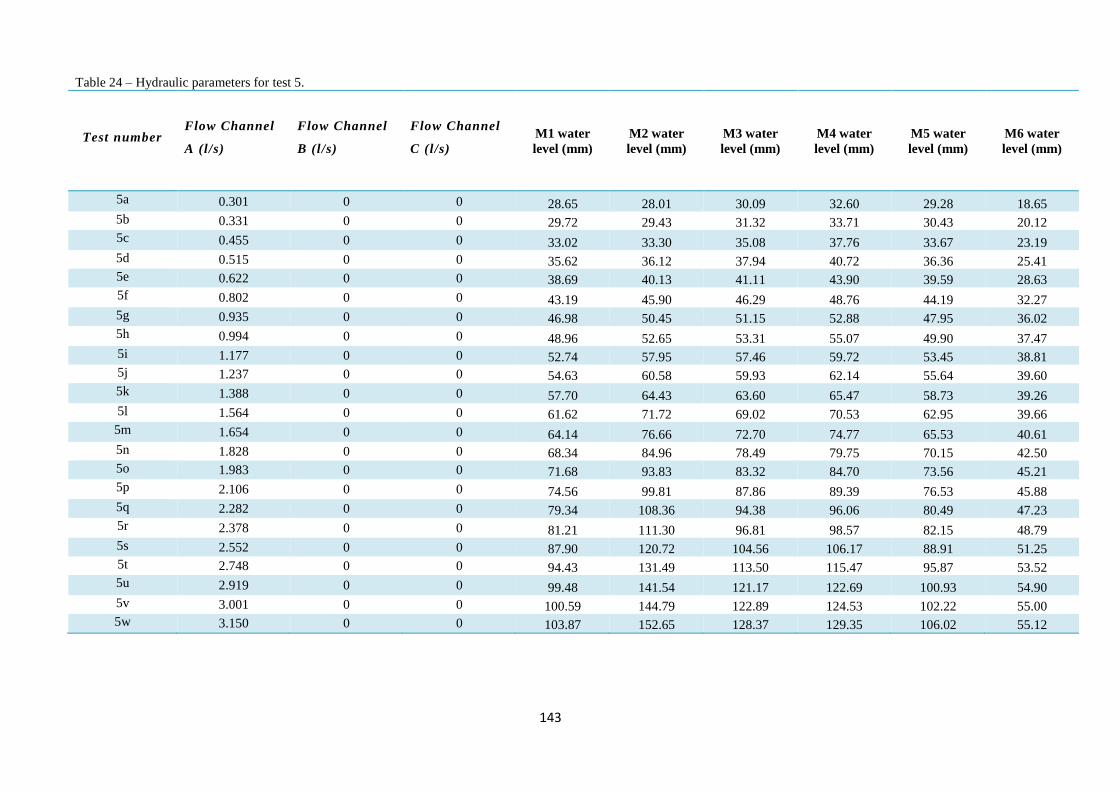
143
Table 24 – Hydraulic parameters for test 5.
Test number Flow Channel
A (l/s)
Flow Channel
B (l/s)
Flow Channel
C (l/s) M1 water
level (mm) M2 water
level (mm) M3 water
level (mm) M4 water
level (mm) M5 water
level (mm)
M6 water
level (mm)
5a 0.301 0 0 28.65 28.01 30.09 32.60 29.28 18.65
5b 0.331 0 0 29.72 29.43 31.32 33.71 30.43 20.12
5c 0.455 0 0 33.02 33.30 35.08 37.76 33.67 23.19
5d 0.515 0 0 35.62 36.12 37.94 40.72 36.36 25.41
5e 0.622 0 0 38.69 40.13 41.11 43.90 39.59 28.63
5f 0.802 0 0 43.19 45.90 46.29 48.76 44.19 32.27
5g 0.935 0 0 46.98 50.45 51.15 52.88 47.95 36.02
5h 0.994 0 0 48.96 52.65 53.31 55.07 49.90 37.47
5i 1.177 0 0 52.74 57.95 57.46 59.72 53.45 38.81
5j 1.237 0 0 54.63 60.58 59.93 62.14 55.64 39.60
5k 1.388 0 0 57.70 64.43 63.60 65.47 58.73 39.26
5l 1.564 0 0 61.62 71.72 69.02 70.53 62.95 39.66
5m 1.654 0 0 64.14 76.66 72.70 74.77 65.53 40.61
5n 1.828 0 0 68.34 84.96 78.49 79.75 70.15 42.50
5o 1.983 0 0 71.68 93.83 83.32 84.70 73.56 45.21
5p 2.106 0 0 74.56 99.81 87.86 89.39 76.53 45.88
5q 2.282 0 0 79.34 108.36 94.38 96.06 80.49 47.23
5r 2.378 0 0 81.21 111.30 96.81 98.57 82.15 48.79
5s 2.552 0 0 87.90 120.72 104.56 106.17 88.91 51.25
5t 2.748 0 0 94.43 131.49 113.50 115.47 95.87 53.52
5u 2.919 0 0 99.48 141.54 121.17 122.69 100.93 54.90
5v 3.001 0 0 100.59 144.79 122.89 124.53 102.22 55.00
5w 3.150 0 0 103.87 152.65 128.37 129.35 106.02 55.12

144
5x 3.267 0 0 106.43 157.52 131.78 132.78 108.75 52.03
5y 3.423 0 0 108.91 165.02 136.35 137.35 111.21 50.31
5z 3.606 0 0 113.95 176.04 144.35 145.00 116.82 51.12
5aa 3.708 0 0 117.62 181.71 149.36 149.81 120.54 51.52
5ab 3.867 0 0 121.59 191.39 155.55 156.32 123.87 51.27
5ac 3.969 0 0 124.22 196.10 158.51 158.68 126.08 51.71
5ad 4.127 0 0 128.40 208.50 166.53 167.29 130.42 51.57
5ae 4.273 0 0 132.17 217.91 171.74 172.72 134.45 51.99
5af 4.394 0 0 136.02 236.04 180.24 181.44 138.71 51.62
5ag 4.540 0 0 141.86 253.05 190.99 192.71 144.33 51.73
5ah 4.706 0 0 147.40 267.94 200.80 202.92 149.78 51.45
5ai 4.815 0 0 151.35 275.38 205.40 207.46 153.77 51.73
5aj 4.966 0 0 159.59 284.09 215.66 216.83 162.46 51.99
5ak 5.148 0 0 168.97 301.62 230.15 233.14 171.61 52.53
5al 5.226 0 0 172.03 308.01 233.74 236.67 174.53 52.77
5am 5.368 0 0 177.80 316.53 240.83 242.80 180.09 53.27
5an 5.543 0 0 186.46 328.15 253.77 256.30 189.01 52.98
5ao 5.650 0 0 190.31 333.26 261.96 264.88 193.23 52.98
5ap 5.761 0 0 194.50 342.15 267.90 270.50 197.77 52.95
5aq 5.878 0 0 201.09 353.47 276.81 278.79 204.46 53.19
5ar 6.002 0 0 205.55 362.56 283.48 284.53 208.99 53.43
5as 6.114 0 0 211.49 373.20 290.93 290.96 215.11 53.12
5at 6.233 0 0 217.63 381.07 296.68 296.50 220.97 52.31
5au 6.374 0 0 225.34 391.04 303.85 302.52 228.15 52.98
5av 6.510 0 0 230.41 398.12 306.02 303.26 232.96 51.62
5aw 6.604 0 0 234.91 405.93 312.57 309.10 237.48 51.19
5ax 6.695 0 0 239.63 415.55 319.28 316.46 242.71 50.70
5ay 6.794 0 0 250.11 432.11 331.88 328.44 252.24 51.12
5az 6.865 0 0 265.86 450.84 348.63 345.38 266.62 50.77

145
Table 25 – Hydraulic parameters for test 6.
Test number
Flow
Channel A
(l/s)
Flow
Channel B
(l/s)
Flow
Channel C
(l/s)
M1 water
level (mm)
M2 water
level (mm)
M3 water
level (mm)
M4 water
level
(mm)
M5 water
level (mm)
M6 water
level (mm)
6a 0 0 0.22 30.60 25.87 27.49 31.50 29.05 15.68
6b 0 0 0.35 33.10 28.24 30.55 33.90 31.29 17.75
6c 0 0 0.48 37.65 32.45 34.80 38.52 35.47 21.57
6d 0 0 0.53 40.82 35.19 37.57 41.40 38.20 23.86
6e 0 0 0.67 45.17 39.86 41.57 45.44 42.79 27.72
6f 0 0 0.80 49.36 43.75 45.51 49.25 46.49 30.74
6g 0 0 0.87 52.08 46.44 48.62 51.85 49.20 32.54
6h 0 0 1.05 56.67 50.30 52.79 56.06 53.00 36.22
6i 0 0 1.210 61.70 55.34 57.77 61.26 58.17 39.29
6j 0 0 1.288 64.24 58.20 60.23 63.61 60.89 39.97
6k 0 0 1.444 68.55 61.82 64.12 67.01 64.34 39.57
6l 0 0 1.594 74.20 66.39 68.83 71.84 69.05 39.36
6m 0 0 1.664 78.50 68.80 70.92 74.20 71.31 40.04
6n 0 0 1.865 86.87 74.18 76.39 79.43 76.10 41.59
6o 0 0 1.957 91.33 77.23 78.92 82.42 79.04 42.92
5p 0 0 2.134 102.24 83.64 85.40 89.38 84.58 43.81
5q 0 0 2.300 111.19 90.42 91.62 95.62 90.09 46.06
5r 0 0 2.410 119.05 95.30 96.58 100.47 94.37 47.46
5s 0 0 2.534 125.49 101.27 102.99 106.71 99.64 48.86
5t 0 0 2.671 134.13 111.05 112.86 116.62 111.62 50.84

146
6u 0 0 2.833 145.00 107.66 109.57 113.06 107.70 50.56
6v 0 0 3.077 156.00 122.66 124.37 127.82 127.77 52.28
6w 0 0 3.310 171.18 130.32 132.07 135.62 137.28 50.38
6x 0 0 3.501 186.17 139.99 141.37 144.96 147.97 47.16
6z 0 0 3.622 194.23 146.83 148.47 151.91 154.27 47.34
6aa 0 0 3.795 207.97 156.95 158.80 162.03 166.07 47.82
6ab 0 0 3.962 225.51 172.11 173.86 176.75 180.34 48.28
6ac 0 0 4.085 236.35 182.88 184.87 187.63 187.39 48.86
6ad 0 0 4.235 248.64 191.70 193.62 196.26 195.39 49.05
6ae 0 0 4.414 262.35 201.68 203.48 206.15 203.78 49.76
6af 0 0 4.530 272.67 209.17 211.48 213.89 212.36 49.63
6ag 0 0 4.677 282.21 218.54 220.64 223.13 221.86 49.98
6ah 0 0 4.785 285.53 227.49 229.90 232.03 231.90 50.13
6ai 0 0 4.927 295.93 236.02 238.34 240.66 241.91 49.98
6aj 0 0 5.120 310.43 248.26 250.31 252.62 256.09 51.09
6ak 0 0 5.232 318.28 255.46 257.61 259.70 265.45 50.60
6al 0 0 5.353 326.65 262.70 264.79 266.53 277.50 50.87
6am 0 0 5.542 341.18 274.28 276.02 277.98 289.11 50.40
6an 0 0 5.656 352.83 282.22 284.13 286.36 296.59 50.66
6ao 0 0 5.758 361.42 288.84 291.07 292.85 303.93 50.05
6ap 0 0 5.935 378.70 300.89 303.24 304.77 317.54 48.94
6aq 0 0 6.071 393.15 311.00 313.39 314.76 327.19 48.60
6ar 0 0 6.187 403.46 318.98 321.49 322.44 338.91 47.20
6as 0 0 6.321 419.84 331.12 333.14 334.91 352.65 47.48

147
6at 0 0 6.445 431.57 339.94 342.76 343.46 362.84 46.23
6au 0 0 6.564 445.27 349.88 352.18 352.95 372.30 45.59
Table 26 – Hydraulic parameters for test 7.
Test number
Flow
Channel A
(l/s)
Flow
Channel B
(l/s)
Flow
Channel C
(l/s)
M1 water
level (mm) M2 water
level (mm) M3 water
level (mm) M4 water
level (mm) M5 water
level (mm)
M6 water
level (mm)
7a 0 0.737 0 42.94 45.02 47.87 49.83 43.76 30.00
7b 0 0.913 0 45.95 49.65 53.12 54.02 46.91 33.75
7c 0 1.215 0 51.66 57.30 60.70 62.02 52.57 37.56
7d 0 1.453 0 58.32 66.39 70.69 70.55 59.45 38.48
7e 0 1.686 0 63.89 74.98 80.89 78.76 65.02 39.69
7f 0 1.940 0 69.82 86.29 98.86 89.39 71.71 43.01
7g 0 2.219 0 76.38 101.19 115.01 102.74 78.09 45.11
7h 0 2.599 0 87.87 119.82 139.24 125.99 89.11 50.54
7i 0 2.836 0 95.94 135.75 160.89 142.15 97.63 53.55
7j 0 3.245 0 105.23 160.07 190.67 166.85 107.20 55.16
7k 0 3.528 0 111.42 178.03 211.61 182.31 113.71 50.77
7l 0 3.789 0 118.98 195.57 234.76 198.59 121.59 49.78
7m 0 4.066 0 126.65 212.99 256.53 215.61 129.11 50.32
7n 0 4.323 0 137.22 234.64 282.34 238.59 140.17 49.65
7o 0 4.569 0 148.10 254.73 297.80 262.86 151.92 49.47
7p 0 4.874 0 160.53 277.68 324.95 286.68 163.87 49.69
7q 0 5.161 0 171.52 300.29 354.35 312.83 175.24 50.19
7r 0 5.409 0 182.82 322.62 381.50 337.14 187.38 50.66
7s 0 5.696 0 198.14 349.99 415.03 367.06 202.17 50.79
7t 0 5.959 0 213.10 377.49 448.88 398.33 216.46 51.18

148
Table 27 – Hydraulic parameters for test 8.
Test number
Flow
Channel A
(l/s)
Flow
Channel B
(l/s)
Flow
Channel C
(l/s)
M1 water
level (mm) M2 water
level (mm) M3 water
level (mm) M4 water
level (mm) M5 water
level (mm)
M6 water
level (mm)
8a 0.859 0 0 45.33 49.02 49.74 51.76 46.69 34.32
8b 1.022 0 0 48.47 53.31 53.41 55.27 49.76 37.27
8c 1.302 0 0 54.43 61.80 60.48 62.65 55.80 38.92
8d 1.612 0 0 61.91 73.24 69.80 71.56 63.39 39.67
8e 1.866 0 0 68.79 89.07 79.61 81.21 70.89 42.73
8f 2.163 0 0 75.41 102.32 89.52 90.87 77.54 45.14
8g 2.450 0 0 82.79 114.00 99.72 100.82 84.14 49.10
8h 2.799 0 0 94.34 133.11 114.75 115.65 96.38 53.75
8i 3.072 0 0 101.39 147.68 124.80 125.85 103.76 55.42
8j 3.289 0 0 104.97 157.97 131.39 132.06 108.01 55.73
8k 3.672 0 0 114.89 179.24 146.18 146.96 118.66 50.73
8l 3.920 0 0 121.25 193.12 155.28 155.51 124.32 50.54
8m 4.179 0 0 128.35 210.91 167.49 167.33 131.25 50.54
8n 4.433 0 0 135.86 242.23 183.24 182.74 139.17 50.67
8o 4.766 0 0 147.59 268.55 200.91 200.41 151.28 50.91
8p 5.016 0 0 161.37 287.79 219.07 218.42 165.31 50.86
8q 5.267 0 0 172.66 309.74 234.98 233.73 175.38 51.64
8r 5.494 0 0 182.17 321.23 248.47 247.04 185.42 51.72
8s 5.826 0 0 195.23 345.49 269.63 267.91 199.58 52.08
8t 6.063 0 0 207.50 368.28 286.20 283.46 212.01 52.02
8u 6.284 0 0 218.93 386.05 298.65 295.98 222.95 52.04
8w 6.534 0 0 230.06 401.87 309.57 306.83 234.01 51.77
8x 6.795 0 0 248.10 429.01 329.82 326.85 250.83 50.73
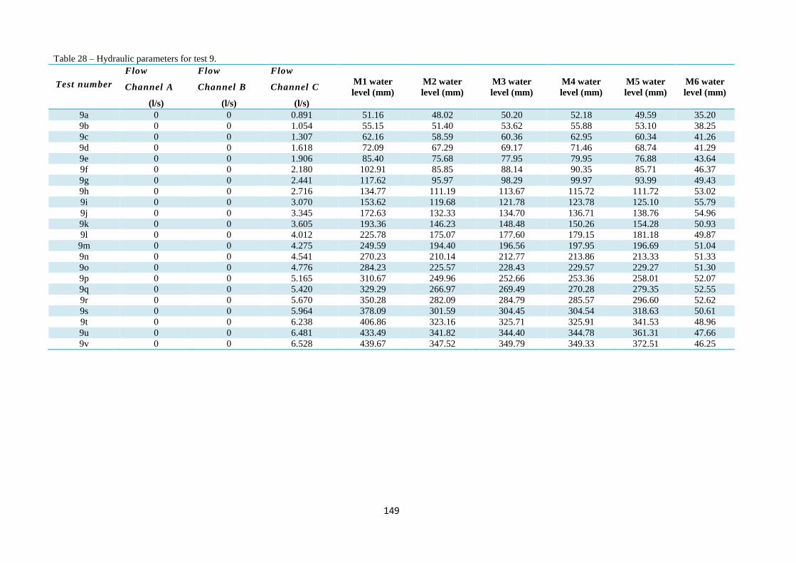
149
Table 28 – Hydraulic parameters for test 9.
Test number
Flow
Channel A
(l/s)
Flow
Channel B
(l/s)
Flow
Channel C
(l/s)
M1 water
level (mm) M2 water
level (mm) M3 water
level (mm) M4 water
level (mm) M5 water
level (mm)
M6 water
level (mm)
9a 0 0 0.891 51.16 48.02 50.20 52.18 49.59 35.20
9b 0 0 1.054 55.15 51.40 53.62 55.88 53.10 38.25
9c 0 0 1.307 62.16 58.59 60.36 62.95 60.34 41.26
9d 0 0 1.618 72.09 67.29 69.17 71.46 68.74 41.29
9e 0 0 1.906 85.40 75.68 77.95 79.95 76.88 43.64
9f 0 0 2.180 102.91 85.85 88.14 90.35 85.71 46.37
9g 0 0 2.441 117.62 95.97 98.29 99.97 93.99 49.43
9h 0 0 2.716 134.77 111.19 113.67 115.72 111.72 53.02
9i 0 0 3.070 153.62 119.68 121.78 123.78 125.10 55.79
9j 0 0 3.345 172.63 132.33 134.70 136.71 138.76 54.96
9k 0 0 3.605 193.36 146.23 148.48 150.26 154.28 50.93
9l 0 0 4.012 225.78 175.07 177.60 179.15 181.18 49.87
9m 0 0 4.275 249.59 194.40 196.56 197.95 196.69 51.04
9n 0 0 4.541 270.23 210.14 212.77 213.86 213.33 51.33
9o 0 0 4.776 284.23 225.57 228.43 229.57 229.27 51.30
9p 0 0 5.165 310.67 249.96 252.66 253.36 258.01 52.07
9q 0 0 5.420 329.29 266.97 269.49 270.28 279.35 52.55
9r 0 0 5.670 350.28 282.09 284.79 285.57 296.60 52.62
9s 0 0 5.964 378.09 301.59 304.45 304.54 318.63 50.61
9t 0 0 6.238 406.86 323.16 325.71 325.91 341.53 48.96
9u 0 0 6.481 433.49 341.82 344.40 344.78 361.31 47.66
9v 0 0 6.528 439.67 347.52 349.79 349.33 372.51 46.25
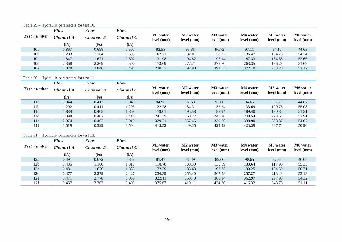
150
Table 29 – Hydraulic parameters for test 10.
Test number
Flow
Channel A
(l/s)
Flow
Channel B
(l/s)
Flow
Channel C
(l/s)
M1 water
level (mm) M2 water
level (mm) M3 water
level (mm) M4 water
level (mm) M5 water
level (mm)
M6 water
level (mm)
10a 0.867 0.698 0.507 82.55 95.31 96.72 97.11 84.10 44.63
10b 1.283 1.164 0.503 102.71 137.01 138.32 136.47 104.78 54.74
10c 1.847 1.671 0.502 131.98 194.82 195.14 187.33 134.55 52.66
10d 2.368 2.269 0.500 173.69 277.71 275.70 263.35 176.23 51.69
10e 3.020 2.846 0.494 230.37 392.90 391.53 372.10 233.20 52.17
Table 30 – Hydraulic parameters for test 11.
Test number
Flow
Channel A
(l/s)
Flow
Channel B
(l/s)
Flow
Channel C
(l/s)
M1 water
level (mm) M2 water
level (mm) M3 water
level (mm) M4 water
level (mm) M5 water
level (mm)
M6 water
level (mm)
11a 0.844 0.412 0.840 84.96 92.58 92.86 94.65 85.88 44.67
11b 1.292 0.411 1.295 122.28 134.31 132.24 133.69 120.75 55.08
11c 1.884 0.405 1.868 179.01 195.58 188.94 189.40 170.85 51.51
11d 2.398 0.402 2.418 241.39 260.27 248.26 248.54 223.63 52.91
11e 2.974 0.402 3.019 329.71 357.45 339.06 338.90 308.37 54.07
11f 3.519 0.399 3.504 415.52 449.35 424.49 423.39 387.74 50.90
Table 31 – Hydraulic parameters for test 12.
Test number
Flow
Channel A
(l/s)
Flow
Channel B
(l/s)
Flow
Channel C
(l/s)
M1 water
level (mm) M2 water
level (mm) M3 water
level (mm) M4 water
level (mm) M5 water
level (mm)
M6 water
level (mm)
12a 0.491 0.672 0.858 81.47 86.49 89.66 90.65 82.33 46.68
12b 0.485 1.180 1.313 118.78 130.30 135.69 133.64 117.90 55.33
12c 0.481 1.670 1.833 172.29 188.63 197.75 190.25 164.50 50.71
12d 0.477 2.279 2.427 236.39 255.40 267.58 257.27 218.43 53.13
12e 0.471 2.778 3.039 322.11 350.40 368.14 362.97 297.93 54.32
12f 0.467 3.307 3.409 375.67 410.11 434.20 416.32 348.76 51.11

151
Table 32 – Hydraulic parameters for test 13.
Test number
Flow
Channel A
(l/s)
Flow
Channel B
(l/s)
Flow
Channel C
(l/s)
M1 water
level (mm) M2 water
level (mm) M3 water
level (mm) M4 water
level (mm) M5 water
level (mm)
M6 water
level (mm)
13a 1.475 1.319 1.498 177.02 208.33 209.96 205.86 171.19 48.08
13b 1.473 1.414 1.500 179.01 213.15 215.94 211.12 173.42 48.24
13c 1.469 1.576 1.497 183.69 222.73 226.91 220.03 178.12 48.23
13d 1.469 1.641 1.498 185.36 226.85 232.28 223.86 179.83 48.16
13e 1.466 1.836 1.496 193.44 240.04 245.60 237.21 188.05 48.50
13f 1.462 1.959 1.491 198.70 249.66 256.89 246.25 193.86 48.82
13g 1.460 2.079 1.485 204.20 259.39 267.10 255.46 199.37 49.49
13h 1.460 2.161 1.487 208.12 263.88 270.87 260.62 203.11 49.74
13i 1.458 2.347 1.484 215.72 276.96 286.51 273.13 211.22 49.76
13j 1.455 2.527 1.485 223.67 289.52 299.31 286.31 219.99 50.61
13k 1.453 2.624 1.481 227.92 296.87 306.41 293.33 223.97 50.36
13l 1.445 2.793 1.481 235.03 315.79 328.20 310.07 231.08 50.31
13m 1.438 2.978 1.473 244.81 332.61 346.25 326.89 241.60 50.74
13n 1.432 3.181 1.474 256.22 358.11 374.32 352.07 253.06 50.60
13o 1.430 3.254 1.470 262.70 372.06 388.43 365.15 259.56 50.23
13p 1.426 3.419 1.471 270.77 387.92 405.89 380.39 267.12 49.56
13q 1.425 3.519 1.470 277.07 399.59 418.71 391.73 273.30 50.39
13r 1.421 3.675 1.466 286.50 416.93 437.15 409.10 282.22 50.36
13s 1.415 3.847 1.461 298.69 438.97 461.17 430.47 294.33 49.91
13t 1.414 3.895 1.456 297.28 440.82 464.81 432.68 294.37 52.04

152
Table 33 – Hydraulic parameters for test 14.
Test number
Flow
Channel A
(l/s)
Flow
Channel B
(l/s)
Flow
Channel C
(l/s)
M1 water
level (mm) M2 water
level (mm) M3 water
level (mm) M4 water
level (mm) M5 water
level (mm)
M6 water
level (mm)
14a 1.421 1.259 1.456 171.60 200.90 202.69 199.19 166.93 49.90
14b 1.526 1.261 1.454 173.35 205.64 206.64 203.34 168.84 50.48
14c 1.606 1.260 1.457 175.81 210.09 210.57 207.17 171.47 50.28
14d 1.794 1.259 1.450 179.64 221.38 220.94 217.49 175.66 50.31
14e 1.976 1.252 1.450 186.22 235.67 233.62 229.83 182.16 50.30
14f 2.048 1.253 1.446 189.91 241.76 239.11 234.54 185.96 50.12
14g 2.238 1.251 1.446 197.64 256.48 249.06 245.40 194.15 50.80
14h 2.306 1.250 1.442 200.97 261.68 252.95 249.34 197.35 50.79
14i 2.489 1.247 1.440 209.27 276.60 264.92 261.22 205.07 50.88
14j 2.678 1.246 1.441 218.66 290.31 277.47 273.74 214.82 51.75
14k 2.870 1.243 1.442 226.89 303.73 289.60 285.82 223.49 51.60
14l 2.937 1.242 1.438 229.55 308.90 294.22 290.48 226.65 51.46
14m 3.119 1.238 1.438 237.68 322.20 305.99 302.41 234.83 51.92
14n 3.200 1.238 1.435 241.69 328.84 312.57 309.06 239.12 51.86
14o 3.366 1.234 1.432 250.03 344.18 324.80 320.71 247.16 51.95
14p 3.528 1.233 1.435 258.79 359.10 338.32 334.36 256.27 51.93
14q 3.626 1.233 1.426 263.96 369.37 346.28 341.60 261.43 51.57
14r 3.773 1.230 1.422 271.92 382.76 357.71 353.85 269.16 51.26
14s 3.881 1.228 1.421 278.48 394.33 367.06 363.38 275.59 51.39
14t 4.029 1.227 1.418 290.21 411.32 381.30 376.96 286.41 50.61
14u 4.187 1.223 1.413 300.69 428.47 396.04 391.72 297.21 50.91
14v 4.280 1.221 1.414 300.78 434.47 399.54 395.36 299.62 49.99
14w 4.427 1.220 1.412 308.59 448.67 411.41 406.88 308.26 50.63
14y 4.476 1.223 1.403 311.99 455.42 416.74 413.17 311.03 48.21
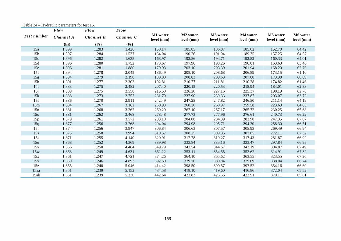
153
Table 34 – Hydraulic parameters for test 15.
Test number
Flow
Channel A
(l/s)
Flow
Channel B
(l/s)
Flow
Channel C
(l/s)
M1 water
level (mm) M2 water
level (mm) M3 water
level (mm) M4 water
level (mm) M5 water
level (mm)
M6 water
level (mm)
15a 1.399 1.283 1.426 158.14 185.85 186.87 185.02 152.70 64.42
15b 1.397 1.284 1.537 164.04 190.26 191.04 189.35 157.25 64.57
15c 1.396 1.282 1.638 168.97 193.86 194.71 192.82 160.33 64.01
15d 1.396 1.280 1.752 173.67 197.96 198.26 196.81 163.63 63.46
15e 1.396 1.281 1.880 179.93 203.10 203.39 201.94 168.20 62.76
15f 1.394 1.278 2.045 186.49 208.10 208.68 206.89 173.15 61.10
15g 1.394 1.279 2.198 188.80 208.83 209.63 207.80 173.38 60.69
15h 1.391 1.277 2.303 192.81 210.77 211.81 210.28 174.82 61.46
14i 1.388 1.275 2.482 207.40 220.15 220.53 218.94 184.01 62.33
15j 1.389 1.275 2.558 215.50 226.20 227.16 225.37 190.19 62.78
15k 1.388 1.273 2.752 231.70 237.90 239.33 237.87 203.07 63.72
15l 1.386 1.270 2.911 242.49 247.25 247.82 246.50 211.14 64.19
15m 1.384 1.267 3.162 260.93 260.30 260.97 259.58 223.63 64.83
15n 1.381 1.268 3.262 269.29 267.10 267.17 265.72 230.25 65.63
15o 1.381 1.262 3.468 278.48 277.73 277.96 276.61 240.73 66.22
15p 1.379 1.261 3.572 283.10 284.08 284.39 282.90 247.35 67.07
15q 1.377 1.256 3.768 294.04 294.98 295.71 294.30 258.30 66.51
15r 1.374 1.256 3.947 306.84 306.63 307.57 305.93 269.49 66.94
15s 1.375 1.258 3.994 310.57 308.25 309.35 307.85 272.11 67.32
15t 1.371 1.255 4.140 320.91 317.78 319.27 317.43 281.87 66.92
15u 1.368 1.252 4.369 339.98 333.84 335.16 333.47 297.84 66.95
15v 1.366 1.250 4.484 349.79 343.54 344.67 343.19 304.87 67.49
15w 1.363 1.249 4.631 362.22 353.11 354.55 352.62 314.91 67.32
15x 1.361 1.247 4.721 374.26 364.10 365.62 363.55 323.55 67.20
15y 1.360 1.246 4.893 392.50 379.70 380.84 379.09 338.04 66.74
15z 1.355 1.240 5.046 414.42 398.50 399.57 397.52 354.16 66.60
15aa 1.351 1.239 5.152 434.58 418.10 419.60 416.86 372.04 65.52
15ab 1.351 1.239 5.230 442.64 423.83 425.55 422.91 379.11 65.81

154
Table 35 – Hydraulic parameters for test 16.
Test number
Flow
Channel A
(l/s)
Flow
Channel B
(l/s)
Flow
Channel C
(l/s)
M1 water
level (mm) M2 water
level (mm) M3 water
level (mm) M4 water
level (mm) M5 water
level (mm)
M6 water
level (mm)
16a 1.419 1.282 1.481 173.49 203.32 204.38 201.29 168.50 48.56
16b 1.413 1.663 1.478 182.21 223.22 227.39 220.80 177.63 49.00
16c 1.406 2.080 1.469 198.91 251.75 258.91 248.21 194.74 49.58
16d 1.401 2.524 1.461 219.28 283.73 294.44 281.00 215.53 50.98
16e 1.393 2.967 1.459 239.57 321.68 336.48 317.01 236.92 50.77
16f 1.381 3.441 1.454 264.95 378.78 397.83 371.70 261.31 50.50
16g 1.372 3.864 1.450 290.19 428.37 451.65 420.72 286.82 49.80
16h 1.368 3.898 1.454 293.58 435.45 458.58 429.95 290.96 49.85
Table 36 – Hydraulic parameters for test 17.
Test number
Flow
Channel A
(l/s)
Flow
Channel B
(l/s)
Flow
Channel C
(l/s)
M1 water
level (mm) M2 water
level (mm) M3 water
level (mm) M4 water
level (mm) M5 water
level (mm)
M6 water
level (mm)
17a 1.388 1.271 1.446 170.37 199.38 200.60 197.37 165.54 48.61
17b 1.826 1.263 1.439 180.75 222.03 219.64 216.83 176.41 49.41
17c 2.278 1.255 1.436 199.04 257.91 248.02 244.48 195.40 50.39
17d 2.720 1.251 1.433 219.52 291.35 278.05 273.80 215.61 50.98
17e 3.143 1.244 1.424 237.88 323.63 306.99 302.93 234.83 51.23
17f 3.569 1.238 1.425 258.38 360.30 337.89 334.01 255.47 50.56
17g 3.886 1.233 1.418 278.14 393.83 366.00 362.02 275.07 50.81
17h 4.292 1.227 1.413 302.54 435.19 400.45 396.36 300.30 50.17
17i 4.541 1.222 1.426 310.83 453.58 412.96 408.68 309.31 49.60

155
Table 37 – Hydraulic parameters for test 18.
Test number
Flow
Channel A
(l/s)
Flow
Channel B
(l/s)
Flow
Channel C
(l/s)
M1 water
level (mm) M2 water
level (mm) M3 water
level (mm) M4 water
level (mm) M5 water
level (mm)
M6 water
level (mm)
18a 1.422 1.245 1.452 171.38 200.30 202.12 198.54 166.72 48.72
18b 1.418 1.241 1.865 191.61 217.11 218.95 215.17 181.82 49.81
18c 1.413 1.232 2.287 227.64 244.87 247.08 243.71 211.25 50.69
18d 1.407 1.228 2.662 258.02 268.87 270.56 267.53 234.63 52.61
18e 1.401 1.223 3.174 292.97 298.93 300.56 297.69 266.70 51.93
18f 1.395 1.218 3.568 319.87 323.92 325.92 322.54 291.71 51.30
18g 1.389 1.211 4.003 360.61 362.97 365.44 361.62 326.90 52.08
18h 1.380 1.202 4.428 416.79 412.49 414.51 410.61 373.24 50.49
18i 1.375 1.202 4.686 449.44 438.00 440.26 436.63 399.33 49.30
Table 38 – Hydraulic parameters for test 19.
Test number
Flow
Channel A
(l/s)
Flow
Channel B
(l/s)
Flow
Channel C
(l/s)
M1 water
level (mm) M2 water
level (mm) M3 water
level (mm) M4 water
level (mm) M5 water
level (mm)
M6 water
level (mm)
19a 1.399 1.268 0.806 129.79 168.84 171.04 167.67 130.13 48.41
19b 1.530 1.388 0.801 134.44 179.65 182.25 177.28 134.92 49.68
19c 1.622 1.545 0.805 141.63 189.65 192.70 185.62 141.99 50.67
19d 1.788 1.628 0.797 149.68 205.01 207.21 199.30 149.81 50.77
19e 1.931 1.799 0.797 159.80 227.30 228.99 220.15 160.59 50.72
19f 2.159 1.922 0.797 173.25 255.39 255.40 243.41 174.29 50.77
19g 2.227 2.027 0.795 181.45 269.68 268.58 258.18 182.42 50.59
19h 2.305 2.191 0.793 193.31 290.23 288.93 277.68 194.75 51.66
19i 2.487 2.261 0.796 205.92 310.45 310.51 299.81 206.55 51.29
19j 2.666 2.468 0.789 223.82 345.42 345.61 331.22 224.45 51.92
19k 2.840 2.646 0.787 241.41 384.76 385.38 367.87 243.10 51.99
19l 2.904 2.737 0.784 250.77 403.60 404.20 384.79 251.81 50.52
19m 3.060 2.928 0.781 271.88 441.59 442.19 421.43 272.87 49.66
19n 3.084 2.952 0.769 278.92 453.69 452.83 431.15 279.20 50.27
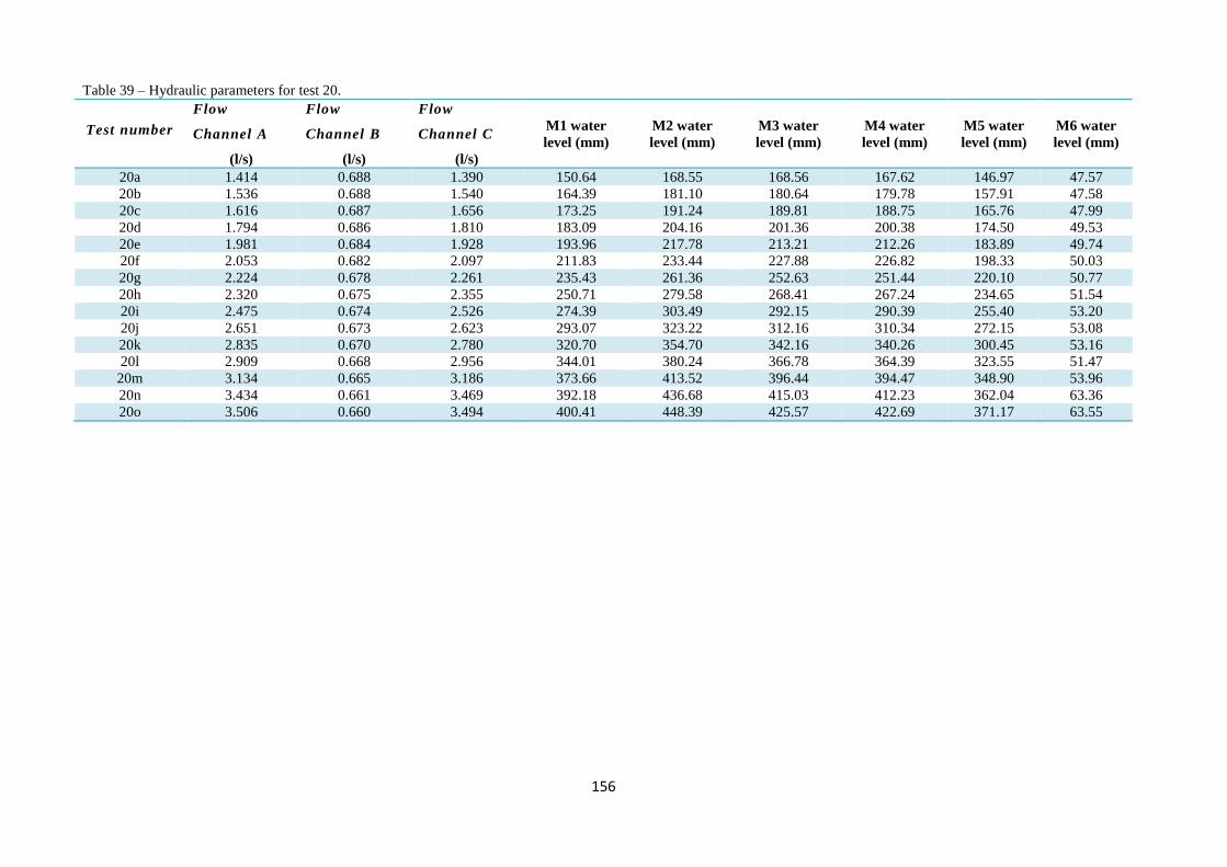
156
Table 39 – Hydraulic parameters for test 20.
Test number
Flow
Channel A
(l/s)
Flow
Channel B
(l/s)
Flow
Channel C
(l/s)
M1 water
level (mm) M2 water
level (mm) M3 water
level (mm) M4 water
level (mm) M5 water
level (mm)
M6 water
level (mm)
20a 1.414 0.688 1.390 150.64 168.55 168.56 167.62 146.97 47.57
20b 1.536 0.688 1.540 164.39 181.10 180.64 179.78 157.91 47.58
20c 1.616 0.687 1.656 173.25 191.24 189.81 188.75 165.76 47.99
20d 1.794 0.686 1.810 183.09 204.16 201.36 200.38 174.50 49.53
20e 1.981 0.684 1.928 193.96 217.78 213.21 212.26 183.89 49.74
20f 2.053 0.682 2.097 211.83 233.44 227.88 226.82 198.33 50.03
20g 2.224 0.678 2.261 235.43 261.36 252.63 251.44 220.10 50.77
20h 2.320 0.675 2.355 250.71 279.58 268.41 267.24 234.65 51.54
20i 2.475 0.674 2.526 274.39 303.49 292.15 290.39 255.40 53.20
20j 2.651 0.673 2.623 293.07 323.22 312.16 310.34 272.15 53.08
20k 2.835 0.670 2.780 320.70 354.70 342.16 340.26 300.45 53.16
20l 2.909 0.668 2.956 344.01 380.24 366.78 364.39 323.55 51.47
20m 3.134 0.665 3.186 373.66 413.52 396.44 394.47 348.90 53.96
20n 3.434 0.661 3.469 392.18 436.68 415.03 412.23 362.04 63.36
20o 3.506 0.660 3.494 400.41 448.39 425.57 422.69 371.17 63.55

157
Table 40 – Hydraulic parameters for test 21.
Test number
Flow
Channel A
(l/s)
Flow
Channel B
(l/s)
Flow
Channel C
(l/s)
M1 water
level (mm) M2 water
level (mm) M3 water
level (mm) M4 water
level (mm) M5 water
level (mm)
M6 water
level (mm)
21a 0.811 1.280 1.459 142.58 158.02 166.24 161.99 137.27 65.45
21b 0.807 1.388 1.596 153.75 171.12 179.73 173.98 146.73 65.72
21c 0.805 1.557 1.673 164.35 185.12 193.94 187.30 156.59 65.49
21d 0.804 1.641 1.832 173.38 194.30 203.02 196.58 163.45 65.16
21e 0.802 1.832 1.937 180.52 205.42 215.42 207.60 169.21 63.63
21f 0.801 1.995 2.116 189.88 216.71 226.82 218.18 175.70 62.20
21g 0.796 2.074 2.271 195.98 222.57 233.22 224.21 179.57 63.17
21h 0.796 2.260 2.356 209.28 237.61 249.51 239.27 190.93 64.61
21i 0.793 2.341 2.508 225.86 251.73 262.56 253.47 203.88 65.50
21j 0.791 2.521 2.599 241.07 271.40 283.58 272.32 217.74 66.32
21k 0.788 2.661 2.756 262.40 294.68 308.25 295.34 236.46 67.03
21l 0.787 2.782 2.904 278.10 316.55 332.52 318.13 252.88 67.80
21m 0.783 2.951 3.069 301.36 346.59 364.24 348.49 274.76 67.64
21n 0.776 3.150 3.163 323.30 378.63 397.22 378.67 297.10 67.30
21o 0.773 3.241 3.344 344.63 403.01 421.72 402.40 317.32 66.73
21p 0.769 3.409 3.436 365.20 428.42 449.26 426.81 334.51 67.07
21q 0.766 3.442 3.446 369.26 435.71 456.62 434.60 339.96 66.23
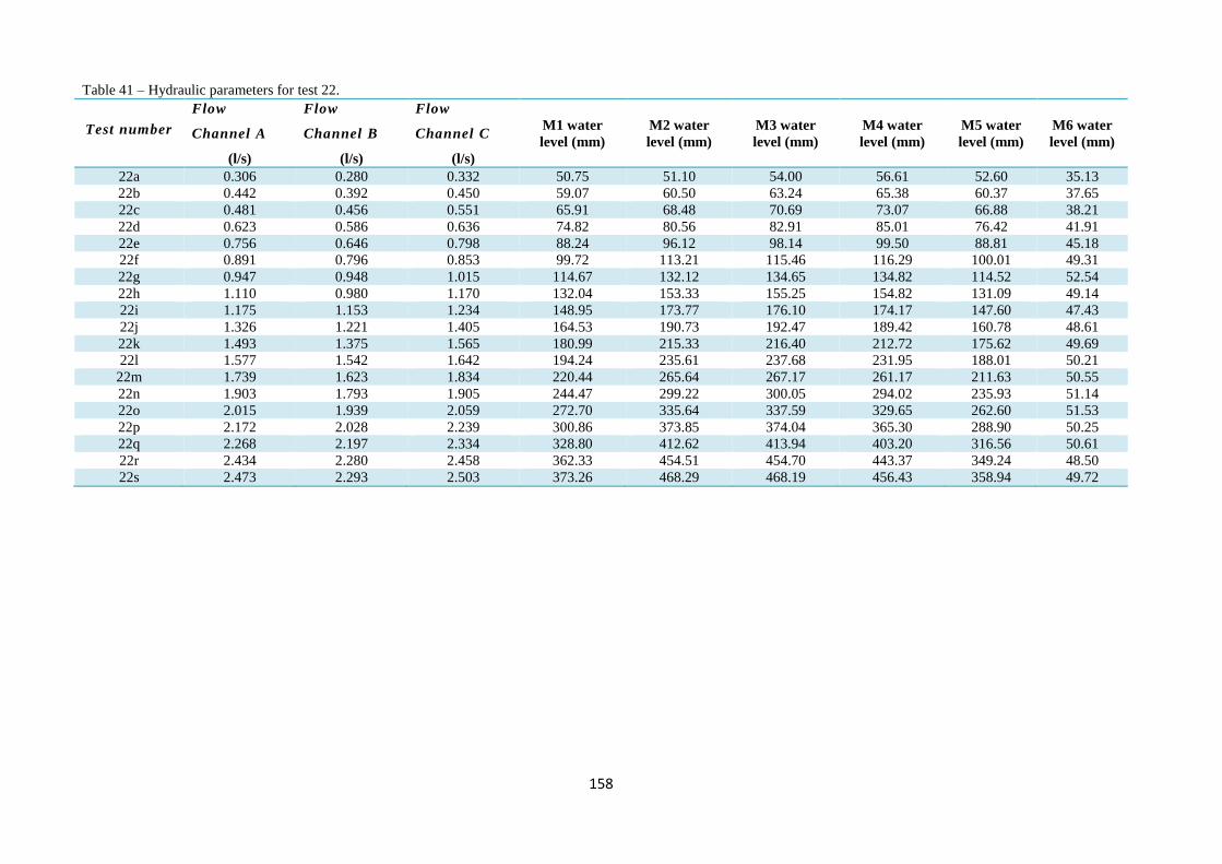
158
Table 41 – Hydraulic parameters for test 22.
Test number
Flow
Channel A
(l/s)
Flow
Channel B
(l/s)
Flow
Channel C
(l/s)
M1 water
level (mm) M2 water
level (mm) M3 water
level (mm) M4 water
level (mm) M5 water
level (mm)
M6 water
level (mm)
22a 0.306 0.280 0.332 50.75 51.10 54.00 56.61 52.60 35.13
22b 0.442 0.392 0.450 59.07 60.50 63.24 65.38 60.37 37.65
22c 0.481 0.456 0.551 65.91 68.48 70.69 73.07 66.88 38.21
22d 0.623 0.586 0.636 74.82 80.56 82.91 85.01 76.42 41.91
22e 0.756 0.646 0.798 88.24 96.12 98.14 99.50 88.81 45.18
22f 0.891 0.796 0.853 99.72 113.21 115.46 116.29 100.01 49.31
22g 0.947 0.948 1.015 114.67 132.12 134.65 134.82 114.52 52.54
22h 1.110 0.980 1.170 132.04 153.33 155.25 154.82 131.09 49.14
22i 1.175 1.153 1.234 148.95 173.77 176.10 174.17 147.60 47.43
22j 1.326 1.221 1.405 164.53 190.73 192.47 189.42 160.78 48.61
22k 1.493 1.375 1.565 180.99 215.33 216.40 212.72 175.62 49.69
22l 1.577 1.542 1.642 194.24 235.61 237.68 231.95 188.01 50.21
22m 1.739 1.623 1.834 220.44 265.64 267.17 261.17 211.63 50.55
22n 1.903 1.793 1.905 244.47 299.22 300.05 294.02 235.93 51.14
22o 2.015 1.939 2.059 272.70 335.64 337.59 329.65 262.60 51.53
22p 2.172 2.028 2.239 300.86 373.85 374.04 365.30 288.90 50.25
22q 2.268 2.197 2.334 328.80 412.62 413.94 403.20 316.56 50.61
22r 2.434 2.280 2.458 362.33 454.51 454.70 443.37 349.24 48.50
22s 2.473 2.293 2.503 373.26 468.29 468.19 456.43 358.94 49.72

159
List of journal papers published
- Rubinato M., Shucksmith J., Saul A.J. “Comparison between Infoworks results and
a physical model of an urban drainage system”, Water Science
and Technology, Vol 68, No 2, pp 372–379.
List of journal papers under review
- Nuno Melo, Leandro J., Shucksmith J., Rubinato M., Djordjevic S., Saul A.J.,
Ramos H., João L. M. P. de Lima, “Evaluation of SIPSON and
SWMM models ability to Reproduce Experimental Data of a
Sewer Network”. Water Science and Technology.
List of journal papers in progress
- Rubinato M., Shucksmith J., Saul A.J. “Quantification of energy losses and flow
exchange between above and below ground drainage systems
through a manhole”. Journal of Hydraulic Engineering.
List of conference papers published
- Rubinato M., Shucksmith J., Saul A.J. “Experimental investigation of flow-
interactions between above and below ground drainage systems
through a manhole”, 17 August 2014- 21 August 2014, 11th
HIC
(International Conference on Hydroinformatics), New York,
USA.
- Lopes P., Shucksmith J., Jorge L., Fernandes de Carvalho R., Rubinato M.
“Velocities profiles and air-entrainment characterization in a
scaled circular manhole”, 7 September 2014- 12 September
2014, 13th
ICUD (International Conference on the Urban
Drainage), Sawarak, MALAYSIA.

160
- Rubinato M., Shucksmith J., Saul A.J. “Comparison between Infoworks results and
a physical model of an urban drainage system”, 3 September
2012- 8 September 2012, 9th
UDM (International Conference on
Urban Drainage Modelling), Belgrade, SERBIA.
- Nuno Melo, Leandro J., Shucksmith J., Rubinato M., Djordjevic Slobodan, Saul A.J.,
Ramos H., João L. M. P. de Lima, “Modelling Internal
Boundary Conditions of a Sewer Network “3 September 2012- 8
September 2012, 9th
UDM (International Conference on Urban
Drainage Modelling), Belgrade, SERBIA.
- Rubinato M., Shucksmith J., Saul A.J. “Procedures for downscaling urban drainage
systems for physical modelling studies”, 14 July 2012- 18 July
2012, 10th
HIC (International Conference on Hydroinformatics),
Hamburg, GERMANY.
- Rubinato M., Shucksmith J., Saul A.J. “Hydraulic performance of a scale model
facility and optimization through the use of real time sensors”,
11 September 2011-17 September 2011, 12th
ICUD (International
Conference on Urban Drainage), Porto Alegre, BRAZIL.