sensors

Article

Geometric Model and Calibration Method for aSolid-State LiDAR

Pablo García-Gómez 1,2,* , Santiago Royo 1,2 , Noel Rodrigo 1,2 and Josep R. Casas 3

1 Centre for Sensors, Instrumentation and Systems Development, Universitat Politècnica de Catalunya(CD6-UPC), Rambla de Sant Nebridi 10, 08222 Terrassa, Spain; santiago.royo@upc.edu (S.R.);noel.rodrigo@upc.edu (N.R.)

2 Beamagine S.L., Carrer de Bellesguard 16, 08755 Castellbisbal, Spain3 Image Processing Group, TSC Department, Universitat Politècnica de Catalunya (UPC), Carrer de Jordi

Girona 1-3, 08034 Barcelona, Spain; josep.ramon.casas@upc.edu* Correspondence: pablo.garcia.gomez@upc.edu

Received: 7 April 2020; Accepted: 18 May 2020; Published: 20 May 2020

Abstract: This paper presents a novel calibration method for solid-state LiDAR devices based on ageometrical description of their scanning system, which has variable angular resolution. Determiningthis distortion across the entire Field-of-View of the system yields accurate and precise measurementswhich enable it to be combined with other sensors. On the one hand, the geometrical model isformulated using the well-known Snell’s law and the intrinsic optical assembly of the system,whereas on the other hand the proposed method describes the scanned scenario with an intuitivecamera-like approach relating pixel locations with scanning directions. Simulations and experimentalresults show that the model fits with real devices and the calibration procedure accurately maps theirvariant resolution so undistorted representations of the observed scenario can be provided. Thus, thecalibration method proposed during this work is applicable and valid for existing scanning systemsimproving their precision and accuracy in an order of magnitude.

Keywords: solid-state LiDAR; LiDAR calibration; distortion correction; FOV mapping

1. Introduction

Nowadays, Light Detection and Ranging (LiDAR) devices are aimed to be used in a widevariety of applications among which autonomous vehicles and computer vision for robotics areoutstanding. Their first studies and uses were related to atmospheric observations [1–3] and airbornemapping [4,5] decades ago. Progressively, the 3D sensing capability of LiDARs pushed them towardsmore user-oriented devices at the same moment in which audiovisual and computer vision applicationssuch as object detection, RGB + depth fusion and augmented reality emerged [6,7].

Furthermore, the current disruption of autonomous driving and robotics has forced LiDARtechnology to move a step forward in order to meet their demanding specifications: large rangeand high spatial resolution whilst real-time performance and background solar tolerance. Initially,mechanical rotating LiDARs [8] showed up as the solution for this technical challenge as theywere based on sending light pulses instead of using amplitude-modulated illumination, prone toproblems with background illumination outdoors. Mechanical LiDARs do imaging through spinninga macroscopic element, either the whole sensor embodiment or an optical element such as a prismor a galvanometer mirror [9]. Nonetheless, moving parts generally mean large enclosures and poormechanical tolerance to vibration, shock and impact. As a consequence, and although they have beenwidely used in research and some industrial applications [10–12], solid-state LiDARs which preciselyavoid large mechanical parts have arisen great interest because they also provide scalability, reliabilityand embeddedness.

Sensors 2020, 20, 2898; doi:10.3390/s20102898 www.mdpi.com/journal/sensors

Sensors 2020, 20, 2898 2 of 23

Currently, several scanning strategies avoiding moving parts are emerging. Due to their constantevolution, there is a vast variety of literature, either scientific publications or patents, concerninghow the scanning method is performed. However, there is no detailed description on how 3D data isactually calculated.

Since new computer vision techniques require accurate and precise 3D representations of thesurroundings of the object for critical applications, there is a real need to provide models and calibrationalgorithms able to correct or compensate any possible distortion in LiDAR scanning. Adding the factthat research is yet mainly based on mechanical techniques, there is a lack of calibration proceduresfor non-mechanical, solid-state devices, in contrast to rotating ones [13–19]. Up to date, significantresearch about LiDAR imaging assumes the LiDAR device provides (x,y,z) data precise enough fromthe direct measurement [20–26].

Thus, the main aim of this work is to present a general-purpose, suitable and understandablescanning model along with a feasible calibration procedure for non-mechanical, solid-state LiDARdevices. In order to do so, the geometry of the system and the sources of distortion will be discussedduring the second section of the paper. Afterwards, the third section will describe the model and thecalibration algorithm proposed as well as the LiDAR devices used for this work. Then, the fourthsection will show the results of the implementation of the suggested method for both devices whereasthe last section will gather the presented results and previous ones for comparison and for reachingconclusions about this work. Two appendixes have been added with the detailed derivation of someof the equations discussed.

2. Problem and Model Formulation

Imaging LiDARs are based on measuring the Time-of-Flight (TOF) value for a number of pointswithin their Field-of-View (FOV). Then, the whole set of points, usually known as point cloud, becomesa 3D representation of the scenario being observed. Without prejudice to the generality and keeping thebroad variety of techniques for either obtaining the TOF measurement and performing the scanning,the nth measured point pn in the LiDAR reference system L can be expressed as follows:

Lpn ≡[Lxn , Lyn , Lzn

]T=

c2

tTOF,n ·L sn, (1)

where c is the speed of light in air, tTOF,n is its TOF measure and sn is the unitary vector representingthe scanning direction of the LiDAR described in its reference system L. From this equation, it canbe appreciated that both the TOF measurement tTOF,n and the scanning direction sn are crucial forobtaining accurate and precise point clouds.

The goal of this paper is to provide a method for characterizing the whole FOV of a solid-stateLiDAR system in order to obtain more accurate and precise point clouds through mapping its angularresolution in detail. As a consequence, this section in particular is going to focus on the scanningdirection of an imaging LiDAR system.

Firstly, the imaging distortion causes will be presented by focusing on a particular solid-stateLiDAR system, which uses a two-axis micro-electrical-mechanical system (MEMS) mirror [27] as areflective surface in order to aim the light beam in both horizontal and vertical directions by steeringon its two axis. Therefore, the mechanics and the dynamics of the scanning system are analyzed on thebasis of vectorial Snell’s law which, eventually, leads us to a non-linear expression relating the twotilting angles of the MEMS with the scanning direction sn. Comparable approaches for obtaining thenon-linear relation between the scanning direction and its scanning principle may be taken for otherscanning methods.

After presenting the distortion causes, a general description of the LiDAR imaging system isgoing to be presented. It is based on a spherical description of the scanning direction and it is suitablefor a broad variety of scanning techniques. This description will be used on the following sections toreach the goal of this paper. Let us start addressing the problem of FOV distortion then.

Sensors 2020, 20, 2898 3 of 23

2.1. The Problem

Ideally, the FOV of the system corresponding to the set of all sn should have constant spacing,meaning constant spatial resolution. Nonetheless, such spacing is distorted as a result of varyingresolution from either optical and/or mechanical mismatch, no matter how the scanning is performed.Thus, a characterization of these undesired artifacts must be done. Generally, it is done using raytracing based in the well-known Snell’s law in combination with some geometrical model of thescanner [14,16,18] as previously introduced.

Snell’s law describes how light is reflected and transmitted at the interface between two mediaof different refractive indices. Thus, it is used in optics to compute those angles and estimate lightpaths [28]. Commonly, it is expressed as a scalar function so a 2D representation is obtained. However,there is an important assumption behind it—the incident and the reflected and/or transmitted rays layin the same plane of the surface normal. Consequently, one of them is a linear combination of the othertwo vectors. Let us describe the reflected ray r as a linear combination of the incident ray i and thesurface normal n, all of them being unitary vectors.

r = µi + ηn. (2)

Vectorial Snell’s law is obtained from the above equation imposing the scalar law and usingvectorial algebra in conjunction with the previously commented assumption. (A detailed derivation ofEquation (3) may be found in Appendix A.1.)

r = µi−(

µ(n · i)−√

1− µ2(1− (n · i)2

))n, (3)

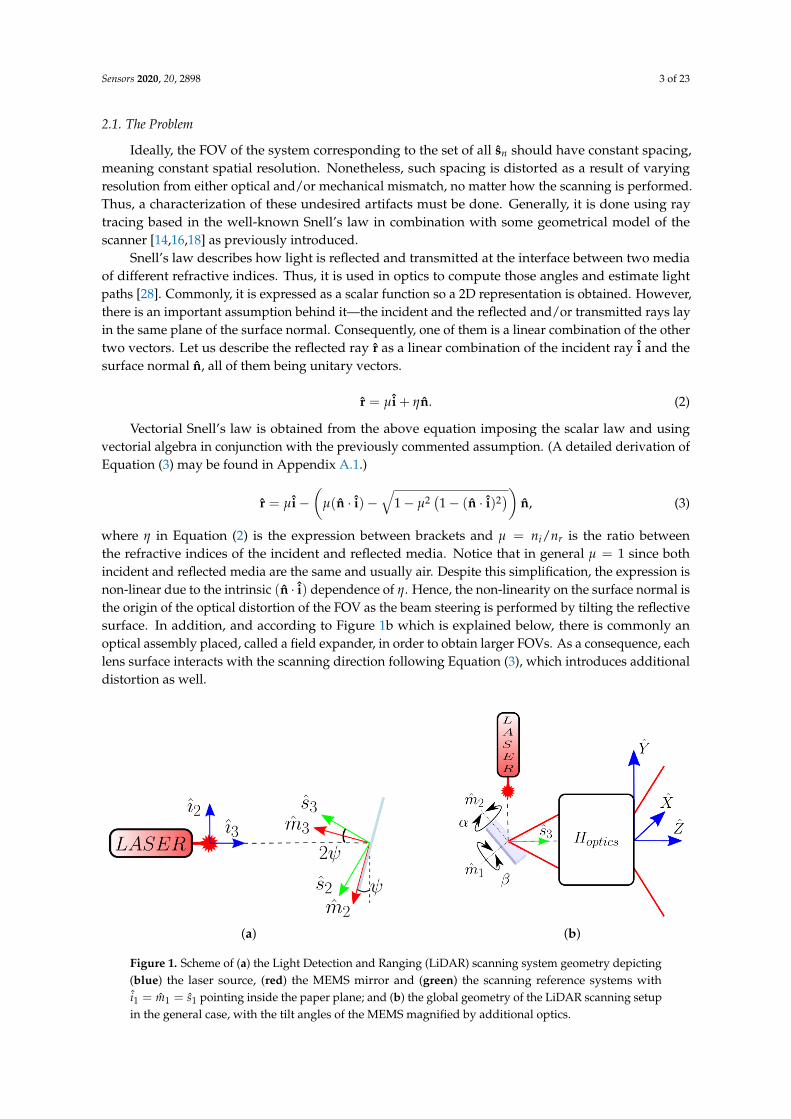
where η in Equation (2) is the expression between brackets and µ = ni/nr is the ratio betweenthe refractive indices of the incident and reflected media. Notice that in general µ = 1 since bothincident and reflected media are the same and usually air. Despite this simplification, the expression isnon-linear due to the intrinsic (n · i) dependence of η. Hence, the non-linearity on the surface normal isthe origin of the optical distortion of the FOV as the beam steering is performed by tilting the reflectivesurface. In addition, and according to Figure 1b which is explained below, there is commonly anoptical assembly placed, called a field expander, in order to obtain larger FOVs. As a consequence, eachlens surface interacts with the scanning direction following Equation (3), which introduces additionaldistortion as well.

(a) (b)

Figure 1. Scheme of (a) the Light Detection and Ranging (LiDAR) scanning system geometry depicting(blue) the laser source, (red) the MEMS mirror and (green) the scanning reference systems withi1 = m1 = s1 pointing inside the paper plane; and (b) the global geometry of the LiDAR scanning setupin the general case, with the tilt angles of the MEMS magnified by additional optics.

Sensors 2020, 20, 2898 4 of 23

Let us now use geometric algebra to express how the tilt angles of the MEMS rotate the surfacenormal n, and consequently, the reflected ray r using Equation (3) which is the scanning direction. Theabove Figure 1 shows the set of reference systems and angles used in the geometrical description of theLiDAR—the reference system of the laser source I, the one for the MEMS or any reflective surface atits resting or central position M, and the one for the scanning optics S.

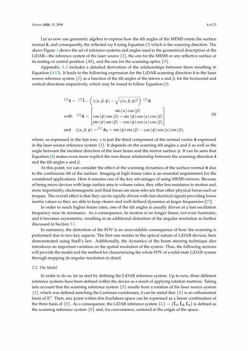
Appendix A.2 includes a detailed derivation of the relationships between them resulting inEquation (A13). It leads to the following expression for the LiDAR scanning direction s in the lasersource reference system I as a function of the tilt angles of the mirror α and β, for the horizontal andvertical directions respectively, which may be found to follow Equation (3).

I s = I i−(

γ(α, β, ψ)−√

γ(α, β, ψ)2)In

with In =

sin (α) cos (β)

cos (ψ) sin (β) + sin (ψ) cos (α) cos (β)

sin (ψ) sin (β)− cos (ψ) cos (α) cos (β)

and γ(α, β, ψ) =I n3 = sin (ψ) sin (β)− cos (ψ) cos (α) cos (β),

(4)

where, as expressed in the last row, γ is just the third component of the normal vector n expressedin the laser source reference system I. It depends on the scanning tilt angles α and β as well as theangle between the incident direction of the laser beam and the mirror surface ψ. It can be seen thatEquation (4) makes even more explicit the non-linear relationship between the scanning direction sand the tilt angles α and β.

At this point, we can consider the effect of the scanning dynamics of the surface normal n dueto the continuous tilt of the surface. Imaging at high frame rates is an essential requirement for theconsidered applications. Here it remains one of the key advantages of using MEMS mirrors. Becauseof being micro devices with large surface area to volume ratios, they offer less resistance to motion and,more importantly, electromagnetic and fluid forces are more relevant than other physical forces such astorques. The overall effect is that they can be rapidly driven with fast electrical signals providing lowerinertia values so they are able to keep clearer and well-defined dynamics at larger frequencies [27].

In order to reach higher frame rates, one of the tilt angles is usually driven at a fast oscillationfrequency near its resonance. As a consequence, its motion is no longer linear, not even harmonic,and it becomes asymmetric, resulting in an additional distortion of the angular resolution as furtherdiscussed in Section 3.1.

In summary, the distortion of the FOV is an unavoidable consequence of how the scanning isperformed due to two key aspects. The first one resides in the optical nature of LiDAR devices, heredemonstrated using Snell’s law. Additionally, the dynamics of the beam steering technique alsointroduces an important variation on the spatial resolution of the system. Thus, the following sectionswill provide the model and the method for characterizing the whole FOV of a solid-state LiDAR systemthrough mapping its angular resolution in detail.

2.2. The Model

In order to do so, let us start by defining the LiDAR reference system. Up to now, three differentreference systems have been defined within the device as a result of applying rotation matrices. Takinginto account that the scanning reference system S results from a rotation of the laser source systemI, which was defined matching the Cartesian coordinates, it can be stated that S is an orthonormalbasis of R3. Then, any point within this Euclidean space can be expressed as a linear combination ofthe three basis of S. As a consequence, the LiDAR reference system L = L1, L2, L3 is defined asthe scanning reference system S and, for convenience, centered at the origin of the space.

Sensors 2020, 20, 2898 5 of 23

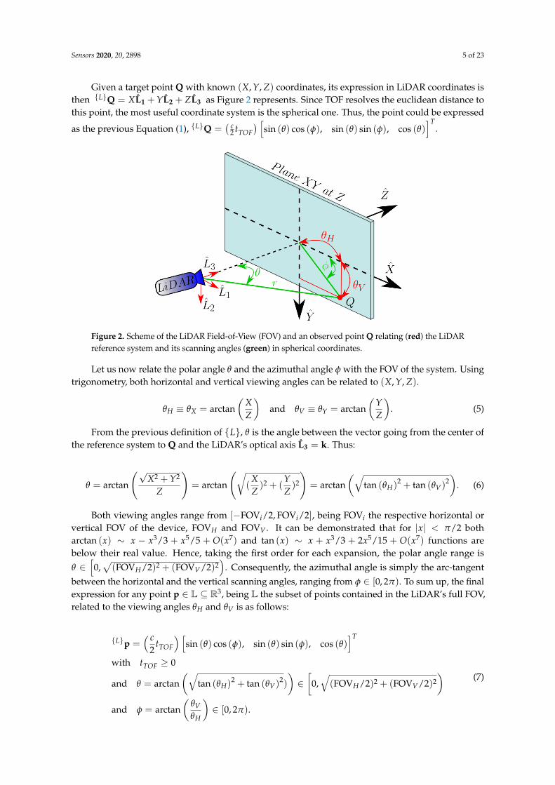
Given a target point Q with known (X, Y, Z) coordinates, its expression in LiDAR coordinates isthen LQ = XL1 + YL2 + ZL3 as Figure 2 represents. Since TOF resolves the euclidean distance tothis point, the most useful coordinate system is the spherical one. Thus, the point could be expressed

as the previous Equation (1), LQ =( c

2 tTOF) [

sin (θ) cos (φ), sin (θ) sin (φ), cos (θ)]T

.

Figure 2. Scheme of the LiDAR Field-of-View (FOV) and an observed point Q relating (red) the LiDARreference system and its scanning angles (green) in spherical coordinates.

Let us now relate the polar angle θ and the azimuthal angle φ with the FOV of the system. Usingtrigonometry, both horizontal and vertical viewing angles can be related to (X, Y, Z).

θH ≡ θX = arctan(

XZ

)and θV ≡ θY = arctan

(YZ

). (5)

From the previous definition of L, θ is the angle between the vector going from the center ofthe reference system to Q and the LiDAR’s optical axis L3 = k. Thus:

θ = arctan

(√X2 + Y2

Z

)= arctan

(√(

XZ)2 + (

YZ)2

)= arctan

(√tan (θH)

2 + tan (θV)2)

. (6)

Both viewing angles range from [−FOVi/2, FOVi/2], being FOVi the respective horizontal orvertical FOV of the device, FOVH and FOVV . It can be demonstrated that for |x| < π/2 botharctan (x) ∼ x − x3/3 + x5/5 + O(x7) and tan (x) ∼ x + x3/3 + 2x5/15 + O(x7) functions arebelow their real value. Hence, taking the first order for each expansion, the polar angle range isθ ∈

[0,√(FOVH/2)2 + (FOVV/2)2

). Consequently, the azimuthal angle is simply the arc-tangent

between the horizontal and the vertical scanning angles, ranging from φ ∈ [0, 2π). To sum up, the finalexpression for any point p ∈ L ⊆ R3, being L the subset of points contained in the LiDAR’s full FOV,related to the viewing angles θH and θV is as follows:

Lp =( c

2tTOF

) [sin (θ) cos (φ), sin (θ) sin (φ), cos (θ)

]T

with tTOF ≥ 0

and θ = arctan(√

tan (θH)2 + tan (θV)

2)

)∈[

0,√(FOVH/2)2 + (FOVV/2)2

)and φ = arctan

(θVθH

)∈ [0, 2π).

(7)

Sensors 2020, 20, 2898 6 of 23

3. Materials and Methods

In this section, we present the method with the scope of mapping both viewing angles θH andθV in order to characterize the varying angular resolution discussed in the previous sections and toprovide reliable point clouds using Equation (7), as well as the tested devices and the calibration target.

3.1. Calibration Method

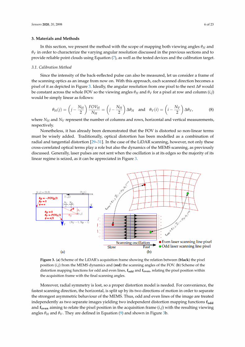
Since the intensity of the back-reflected pulse can also be measured, let us consider a frame ofthe scanning optics as an image from now on. With this approach, each scanned direction becomes apixel of it as depicted in Figure 3. Ideally, the angular resolution from one pixel to the next ∆θ wouldbe constant across the whole FOV so the viewing angles θH and θV for a pixel at row and column (i,j)would be simply linear as follows:

θH(j) =(

j− NH2

)FOVH

NH=

(j− NH

2

)∆θH and θV(i) =

(i− NV

2

)∆θV , (8)

where NH and NV represent the number of columns and rows, horizontal and vertical measurements,respectively.

Nonetheless, it has already been demonstrated that the FOV is distorted so non-linear termsmust be wisely added. Traditionally, optical distortion has been modelled as a combination ofradial and tangential distortion [29–31]. In the case of the LiDAR scanning, however, not only thesecross-correlated optical terms play a role but also the dynamics of the MEMS scanning, as previouslydiscussed. Generally, laser pulses are not sent when the oscillation is at its edges so the majority of itslinear regime is seized, as it can be appreciated in Figure 3.

Figure 3. (a) Scheme of the LiDAR’s acquisition frame showing the relation between (black) the pixelposition (i,j) from the MEMS dynamics and (red) the scanning angles of the FOV. (b) Scheme of thedistortion mapping functions for odd and even lines, fodd and feven, relating the pixel position withinthe acquisition frame with the final scanning angles.

Moreover, radial symmetry is lost, so a proper distortion model is needed. For convenience, thefastest scanning direction, the horizontal, is split up by its two directions of motion in order to separatethe strongest asymmetric behaviour of the MEMS. Thus, odd and even lines of the image are treatedindependently as two separate images yielding two independent distortion mapping functions foddand feven aiming to relate the pixel position in the acquisition frame (i,j) with the resulting viewingangles θH and θV . They are defined in Equation (9) and shown in Figure 3b.

Sensors 2020, 20, 2898 7 of 23

Following the literature about distortion mapping [32–34], different nonlinear equations wereproposed and tested along the development of this work and are presented in the following Section 3.2.Defining ı = (i− NV/2) and = (j− NH/2) and both

−→A and

−→B as the vectors containing the set of

parameters for both odd and even horizontal scanning directions respectively, the two viewing anglesmay be expressed, without loss of generality, as:

f : (i, j)−→X7−→ (θH , θV)

[θH(i, j)

θV(i, j)

]odd

= f(ı, ,−→A ) ≡ fodd[

θH(i, j)

θV(i, j)

]even

= f(ı, ,−→B ) ≡ feven.

(9)

Now, finding both mapping functions fodd and feven reduces to solving a non-linear least squaressystem (NLSQ) for a set of M control viewing angles θm

H and θmV measured at different pixel positions

(im, jm), so both vector parameters−→A and

−→B minimize an objective function g. Our suggested objective

function is based on the angular error between the control viewing angles and the estimated ones at themeasured pixel positions on the image using the mapping functions fodd and feven, as expressed below.

−→A ,−→B | min−→

X||gk(im, jm,

−→X )||22 = min−→

X||[

θmH

θmV

]k

− fk(im, jm,−→X )||22 =

= min−→X

M

∑m=1||[

θmH − θH

θmV − θV

]k

||22 ∀m = 1, .., M with k = odd, even.(10)

3.2. Distortion Mapping Equations

Let us now introduce the three different sets of mapping functions fk (with k = odd, even) thathave been proposed and tested during this work. As previously commented, the mapping functionsaim to model the discussed angular variation that causes the FOV distortion. Thus, non-linearterms must be added to the ideal linear case presented in Equation (8) where the angular resolutionis constant.

According to this, the linear term has been expanded up to a third-order polynomial in orderto include the effect of the varying angular velocity and acceleration of the MEMS. This expansionis common to all the proposed mapping functions and relates exclusively the effect on the scanningdirection, horizontal or vertical, caused by its corresponding pixel direction on the image.

On one hand, θH,0 and θV,0 apply for a global shift of the viewing angles in each direction. Onthe other hand, ∆θH and ∆θV can be considered as the mean angular resolution as if the FOV washomogeneous. Then, the following non-linear terms are related to the MEMS scanning dynamics,being ωH and ωV related to the MEMS angular velocities due to their even symmetry whereas ΩHand ΩV are related to its angular acceleration because of their odd symmetry.

Firstly, an equation similar to the widely used optical distortion model [35] is proposed. Thismodel introduces a radial distortion with terms proportional to the radial distance to the centerof the image plus a couple of cross-correlated terms with a distortion center in pixels known asthe tangential distortion. However, since the MEMS dynamics is asymmetric, we have introducedintroduced different cross-correlated terms following the literature about distortion mapping for opticaldisplays [32–34] that provide a higher degree-of-freedom (DOF) to the cross-effect of the scanningdirections than the traditional imaging distortion model used in the first approach.

Then, the second and the third proposed mapping functions contain the same number ofcross-correlated terms, three in particular, but they differ in the DOF given to the optical distortioncenters in pixels. Whereas the second one presents a unique distortion center for all the terms, thethird one has different individual distortion centers for each term becoming the mapping functionwith the highest DOF possible.

Sensors 2020, 20, 2898 8 of 23

Once the common part of the three proposed mapping functions has been discussed as well asthe inclusion of the cross-correlated terms, let us now introduce them separately in detail. Recall thatthe pixel positions are normalized as ı = (i− NV/2) and = (j− NH/2).

Map 1: Optical-Like Mapping

Defining the radius as r = ı2 + 2, the radial Rn and tangential Pn traditional optical coefficientsare applied with a common distortion center on the image ic and jc.

fkM1 : (i, j)

−→X7−→ (θH , θV)

θH(i, j) =θH,0 + ∆θH ( + jc) + ωH ( + jc)2 + ΩH ( + jc)

3 +

+R1r + R2r2 + R3r4 + P1

(r + 2 ( + jc)

2)+ 2P2 ( + jc) (ı + ic)

θV(i, j) =θV,0 + ∆θV (ı + ic) + ωV (ı + ic)2 + ΩV ( + ic)

3 +

+R1r + R2r2 + R3r4 + 2P1 ( + jc) (ı + ic) + P2

(r + 2 (ı + ic)

2)

.

(11)

Map 2: Cross Mapping

Instead of using the traditional distortion coefficients, the cross-terms are introduced with moregeneral functions but using the same common distortion center. PH,n apply for the cross-terms affectingθH whereas PV,n for θV .

fkM2 : (i, j)

−→X7−→ (θH , θV)

θH(i, j) =θH,0 + ∆θH ( + jc) + ωH ( + jc)2 + ΩH ( + jc)

3 +

+PH,1 ( + jc) (ı + ic) + PH,2 ( + jc)2 (ı + ic) + PH,3 ( + jc) (ı + ic)

2

θV(i, j) =θV,0 + ∆θV (ı + ic) + ωV (ı + ic)2 + ΩV (ı + ic)

3 +

+PV,1 ( + jc) (ı + ic) + PV,2 ( + jc)2 (ı + ic) + PV,3 ( + jc) (ı + ic)

2 .

(12)

Map 3: Multi-Decentered Cross-Mapping

Finally, rather than using a unique distortion center on the image for all functions, this equationprovides freedom to every term to have a specific distortion center.

fkM3 : (i, j)

−→X7−→ (θH , θV)

θH(i, j) =θH,0 + ∆θH ( + j0) + ωH ( + jω0)2 + ΩH ( + jΩ0)

3 +

+PH,1 ( + jP1) (ı + iP1) + PH,2 ( + jP2)2 (ı + iP2) + PH,3 ( + jP3) (ı + iP3)

2

θV(i, j) =θV,0 + ∆θV (ı + i0) + ωV (ı + iω0)2 + ΩV (ı + iΩ0)

3 +

+PV,1 ( + jP1) (ı + iP1) + PV,2 ( + jP2)2 (ı + iP2) + PV,3 ( + jP3) (ı + iP3)

2 .

(13)

3.3. Calibration Pattern and Algorithm

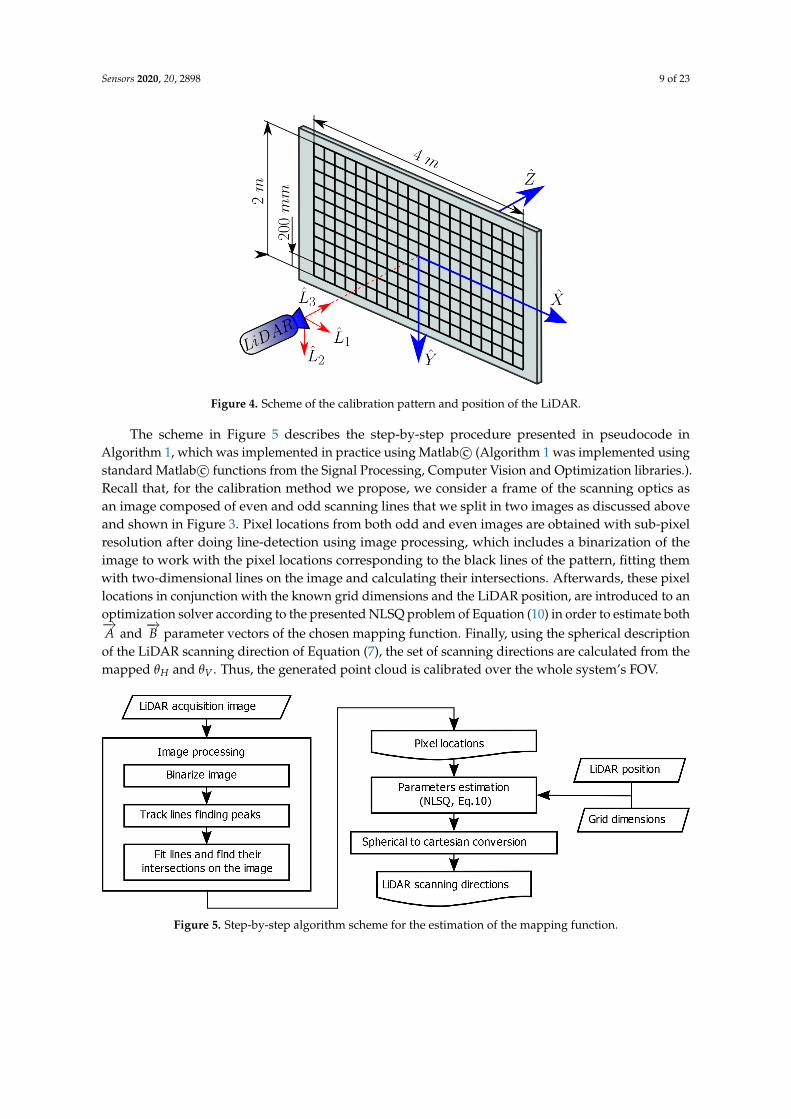
In order to obtain the set of measurements, a regular grid of dimension 4 × 2 m with 200 mmwidth squares was constructed onto a planar wall with absorbent optical duct tape as depicted inFigure 4. Then, the LiDAR prototype is placed at a known Z distance facing the pattern so bothviewing angles can be resolved using Equation (5) for all the scanned grid’s intersections.

Sensors 2020, 20, 2898 9 of 23

Figure 4. Scheme of the calibration pattern and position of the LiDAR.

The scheme in Figure 5 describes the step-by-step procedure presented in pseudocode inAlgorithm 1, which was implemented in practice using Matlab c© (Algorithm 1 was implemented usingstandard Matlab c© functions from the Signal Processing, Computer Vision and Optimization libraries.).Recall that, for the calibration method we propose, we consider a frame of the scanning optics asan image composed of even and odd scanning lines that we split in two images as discussed aboveand shown in Figure 3. Pixel locations from both odd and even images are obtained with sub-pixelresolution after doing line-detection using image processing, which includes a binarization of theimage to work with the pixel locations corresponding to the black lines of the pattern, fitting themwith two-dimensional lines on the image and calculating their intersections. Afterwards, these pixellocations in conjunction with the known grid dimensions and the LiDAR position, are introduced to anoptimization solver according to the presented NLSQ problem of Equation (10) in order to estimate both−→A and

−→B parameter vectors of the chosen mapping function. Finally, using the spherical description

of the LiDAR scanning direction of Equation (7), the set of scanning directions are calculated from themapped θH and θV . Thus, the generated point cloud is calibrated over the whole system’s FOV.

Figure 5. Step-by-step algorithm scheme for the estimation of the mapping function.

Sensors 2020, 20, 2898 10 of 23

Algorithm 1: Image processing for obtaining the pixel locations of the lines’ intersections.

Input: LiDAR acquisition intensity image I(i, j) of Nrows and Ncols dimensions.Output: Pixel locations of the lines’ intersections pm = (im, jm)

1 Binarize image applying an intensity threshold value Ithd:2 for i = 1 to Nrows do3 for j = 1 to Ncols do4 if I(i, j) ≤ Ithd then5 IB(i, j) = 1

6 else7 IB(i, j) = 0.

8 For each horizontal and vertical direction, get the number of lines N, their expected pixelposition pl and width wl using peak analysis on a certain row iini and column jini of IB(i, j) :

9 Nhor ← number of peaks in IB(i = 1 to Nrows , jini)

10 for each peak lh = 1 to Nhor in IB(i = 1 to Nrows , jini) do11 ilh ← row position ilh of the lth-peak in IB(i = 1 to Nrows , jini)

12 plh ← peak position (ilh, jini)

13 wlh ← width of the lth-peak in pixels (rows of the peak)

14 Nver ← number of peaks in IB(iini , j = 1 to Ncols)

15 for each peak lv = 1 to Nver in IB(iini , j = 1 to Ncols) do16 jlv ← column position jlv of the lth-peak in IB(iini , j = 1 to Ncols)

17 plv ← peak position (iini, jlv)18 wlv ← width of the lth-peak in pixels (columns of the peak).

19 Track each line Lk scanning the image to obtain the set of pixel locations within its width wLand fit a 3rd order polynomial Llh ≡ y = a0 + a1x + a2x2 + a3x3 using least squares:

20 for each horizontal line lh = 1 to Nhor do21 for j = 1 to Ncols do22 if IB(ilh ± wlh

2 , j) = 1 then23 Llh ← (ilh ± wlh

2 , j)

24 Llh(i, j)← i = a0 + a1 j + a2 j2 + a3 j3 for j ∈ 1 to Ncols

25 for each vertical line lv = 1 to Nver do26 for i = 1 to Nrows do27 if IB(i , jlv ± wlv

2 ) = 1 then28 Llv ← (i , jlv ± wlv

2 )

29 Llv(i, j)← j = a0 + a1i + a2i2 + a3i3 for i ∈ 1 to Nrows

30 Find the pixel location of the intersection pm = (im, jm) between each pair of horizontal Llh

and vertical Llv lines:31 for each horizontal line lh = 1 to Nhor do32 for each vertical line lv = 1 to Nver do33 pm ← ||Llh(im, jm)− Llv(im, jm)||2 = 0.

3.4. Prototypes

With the purpose of testing the method with different FOVs and distortions, two long rangesolid-state LiDAR prototypes from Beamagine S.L. with different FOV have been used. For the firstone, we used a 30 × 20 FOV prototype with 300 × 150 pixels (45 k points) whereas for the secondone, we used a 50 × 20 FOV with 500 × 150 pixels (75 k points).

Sensors 2020, 20, 2898 11 of 23

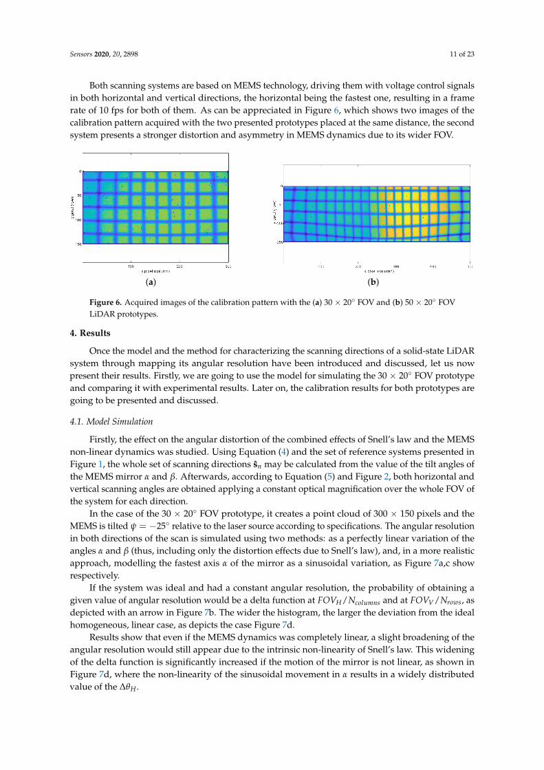
Both scanning systems are based on MEMS technology, driving them with voltage control signalsin both horizontal and vertical directions, the horizontal being the fastest one, resulting in a framerate of 10 fps for both of them. As can be appreciated in Figure 6, which shows two images of thecalibration pattern acquired with the two presented prototypes placed at the same distance, the secondsystem presents a stronger distortion and asymmetry in MEMS dynamics due to its wider FOV.

(a) (b)

Figure 6. Acquired images of the calibration pattern with the (a) 30 × 20 FOV and (b) 50 × 20 FOVLiDAR prototypes.

4. Results

Once the model and the method for characterizing the scanning directions of a solid-state LiDARsystem through mapping its angular resolution have been introduced and discussed, let us nowpresent their results. Firstly, we are going to use the model for simulating the 30 × 20 FOV prototypeand comparing it with experimental results. Later on, the calibration results for both prototypes aregoing to be presented and discussed.

4.1. Model Simulation

Firstly, the effect on the angular distortion of the combined effects of Snell’s law and the MEMSnon-linear dynamics was studied. Using Equation (4) and the set of reference systems presented inFigure 1, the whole set of scanning directions sn may be calculated from the value of the tilt angles ofthe MEMS mirror α and β. Afterwards, according to Equation (5) and Figure 2, both horizontal andvertical scanning angles are obtained applying a constant optical magnification over the whole FOV ofthe system for each direction.

In the case of the 30 × 20 FOV prototype, it creates a point cloud of 300 × 150 pixels and theMEMS is tilted ψ = −25 relative to the laser source according to specifications. The angular resolutionin both directions of the scan is simulated using two methods: as a perfectly linear variation of theangles α and β (thus, including only the distortion effects due to Snell’s law), and, in a more realisticapproach, modelling the fastest axis α of the mirror as a sinusoidal variation, as Figure 7a,c showrespectively.

If the system was ideal and had a constant angular resolution, the probability of obtaining agiven value of angular resolution would be a delta function at FOVH/Ncolumns and at FOVV/Nrows, asdepicted with an arrow in Figure 7b. The wider the histogram, the larger the deviation from the idealhomogeneous, linear case, as depicts the case Figure 7d.

Results show that even if the MEMS dynamics was completely linear, a slight broadening of theangular resolution would still appear due to the intrinsic non-linearity of Snell’s law. This wideningof the delta function is significantly increased if the motion of the mirror is not linear, as shown inFigure 7d, where the non-linearity of the sinusoidal movement in α results in a widely distributedvalue of the ∆θH .

Sensors 2020, 20, 2898 12 of 23

Figure 7. Simulated probability histogram of the angular resolution (b) and (d) for both scanningdirections assuming, respectively, (a) linear motion of the MEMS and (c) harmonic motion of the MEMSin its fastest direction, being the red curve of α the cropped linear region of the whole motion shown inblue. Homogeneous resolution is calculated with FOVH = 27.5 and FOVV = 16.5.

To further depict the effect, the resulting image from scanning the calibration pattern from aknown distance of 3.8 m is simulated and qualitatively compared to an experimental capture. Thiscomparison is going to become quantitative later on whilst comparing the angular resolutions acrossthe whole FOV and in Section 4.3 as well. Both images are shown in Figure 8. Both of them presentcurves instead of straight lines as a result of fluctuation in angular resolution due to the differentnon-linearities in the system, as expected. Notice also how vertical lines are specially modified atthe bottom of the image, where they bend towards the center, suggesting that not only the fast axisof the MEMS mirror, but also the slow one, present a non-linear behavior, as will be discussed later.Moreover, the asymmetric behaviour between odd and even rows of the image can be appreciated.

Figure 8. (a) Simulated and (b) experimental image of the grid pattern at 3.8 m using the 30 × 20 FOVprototype.

4.2. Calibration Results

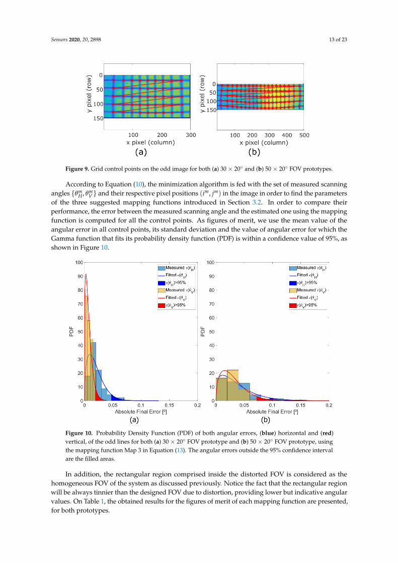
After simulating the model, we place the two prototypes being considered at a known distanceof 3.8 m from the grid pattern described in Section 3, in order to test the calibration algorithm. Thegrid lines on the image are tracked and fitted, resulting in respectively 45 and 95 intersections for eachLiDAR prototype as Figure 9 shows, which are the measured pixel positions (im, jm).

Sensors 2020, 20, 2898 13 of 23

Figure 9. Grid control points on the odd image for both (a) 30 × 20 and (b) 50 × 20 FOV prototypes.

According to Equation (10), the minimization algorithm is fed with the set of measured scanningangles θm

H , θmV and their respective pixel positions (im, jm) in the image in order to find the parameters

of the three suggested mapping functions introduced in Section 3.2. In order to compare theirperformance, the error between the measured scanning angle and the estimated one using the mappingfunction is computed for all the control points. As figures of merit, we use the mean value of theangular error in all control points, its standard deviation and the value of angular error for which theGamma function that fits its probability density function (PDF) is within a confidence value of 95%, asshown in Figure 10.

Figure 10. Probability Density Function (PDF) of both angular errors, (blue) horizontal and (red)vertical, of the odd lines for both (a) 30 × 20 FOV prototype and (b) 50 × 20 FOV prototype, usingthe mapping function Map 3 in Equation (13). The angular errors outside the 95% confidence intervalare the filled areas.

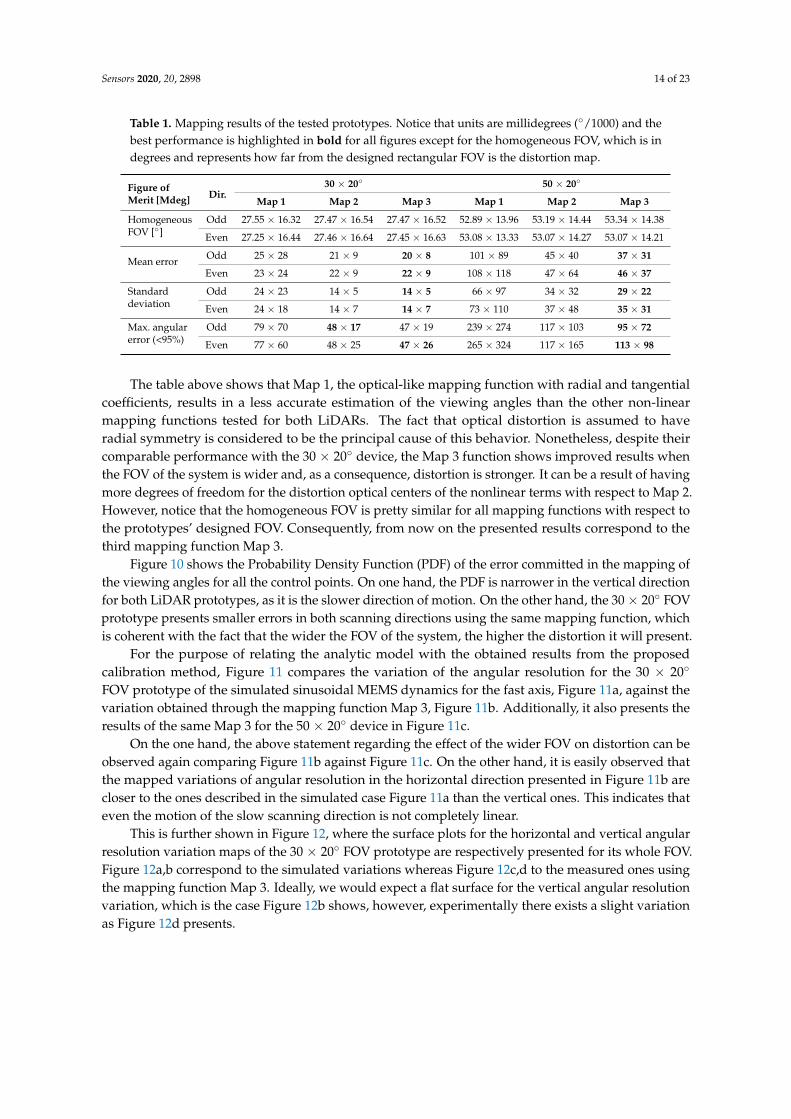
In addition, the rectangular region comprised inside the distorted FOV is considered as thehomogeneous FOV of the system as discussed previously. Notice the fact that the rectangular regionwill be always tinnier than the designed FOV due to distortion, providing lower but indicative angularvalues. On Table 1, the obtained results for the figures of merit of each mapping function are presented,for both prototypes.

Sensors 2020, 20, 2898 14 of 23

Table 1. Mapping results of the tested prototypes. Notice that units are millidegrees (/1000) and thebest performance is highlighted in bold for all figures except for the homogeneous FOV, which is indegrees and represents how far from the designed rectangular FOV is the distortion map.

Figure ofMerit [Mdeg] Dir.

30 × 20 50 × 20

Map 1 Map 2 Map 3 Map 1 Map 2 Map 3

HomogeneousFOV []

Odd 27.55 × 16.32 27.47 × 16.54 27.47 × 16.52 52.89 × 13.96 53.19 × 14.44 53.34 × 14.38

Even 27.25 × 16.44 27.46 × 16.64 27.45 × 16.63 53.08 × 13.33 53.07 × 14.27 53.07 × 14.21

Mean error Odd 25 × 28 21 × 9 20 × 8 101 × 89 45 × 40 37 × 31

Even 23 × 24 22 × 9 22 × 9 108 × 118 47 × 64 46 × 37

Standarddeviation

Odd 24 × 23 14 × 5 14 × 5 66 × 97 34 × 32 29 × 22

Even 24 × 18 14 × 7 14 × 7 73 × 110 37 × 48 35 × 31

Max. angularerror (<95%)

Odd 79 × 70 48 × 17 47 × 19 239 × 274 117 × 103 95 × 72

Even 77 × 60 48 × 25 47 × 26 265 × 324 117 × 165 113 × 98

The table above shows that Map 1, the optical-like mapping function with radial and tangentialcoefficients, results in a less accurate estimation of the viewing angles than the other non-linearmapping functions tested for both LiDARs. The fact that optical distortion is assumed to haveradial symmetry is considered to be the principal cause of this behavior. Nonetheless, despite theircomparable performance with the 30 × 20 device, the Map 3 function shows improved results whenthe FOV of the system is wider and, as a consequence, distortion is stronger. It can be a result of havingmore degrees of freedom for the distortion optical centers of the nonlinear terms with respect to Map 2.However, notice that the homogeneous FOV is pretty similar for all mapping functions with respect tothe prototypes’ designed FOV. Consequently, from now on the presented results correspond to thethird mapping function Map 3.

Figure 10 shows the Probability Density Function (PDF) of the error committed in the mapping ofthe viewing angles for all the control points. On one hand, the PDF is narrower in the vertical directionfor both LiDAR prototypes, as it is the slower direction of motion. On the other hand, the 30× 20 FOVprototype presents smaller errors in both scanning directions using the same mapping function, whichis coherent with the fact that the wider the FOV of the system, the higher the distortion it will present.

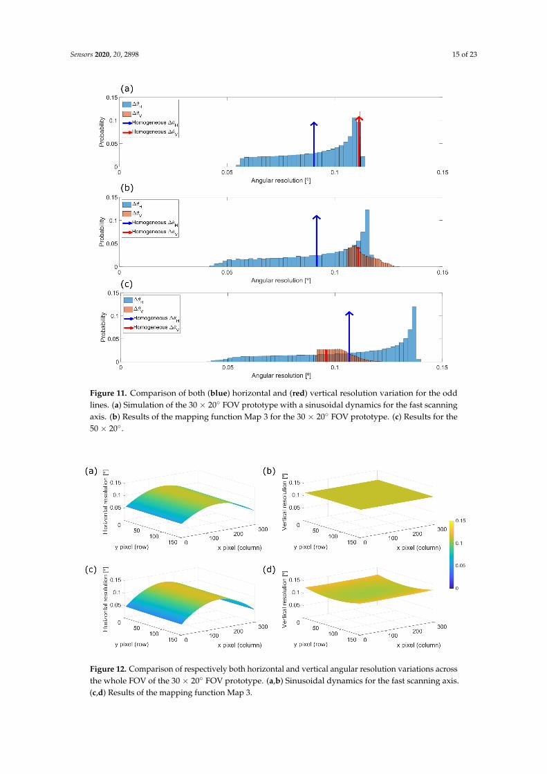
For the purpose of relating the analytic model with the obtained results from the proposedcalibration method, Figure 11 compares the variation of the angular resolution for the 30 × 20

FOV prototype of the simulated sinusoidal MEMS dynamics for the fast axis, Figure 11a, against thevariation obtained through the mapping function Map 3, Figure 11b. Additionally, it also presents theresults of the same Map 3 for the 50 × 20 device in Figure 11c.

On the one hand, the above statement regarding the effect of the wider FOV on distortion can beobserved again comparing Figure 11b against Figure 11c. On the other hand, it is easily observed thatthe mapped variations of angular resolution in the horizontal direction presented in Figure 11b arecloser to the ones described in the simulated case Figure 11a than the vertical ones. This indicates thateven the motion of the slow scanning direction is not completely linear.

This is further shown in Figure 12, where the surface plots for the horizontal and vertical angularresolution variation maps of the 30 × 20 FOV prototype are respectively presented for its whole FOV.Figure 12a,b correspond to the simulated variations whereas Figure 12c,d to the measured ones usingthe mapping function Map 3. Ideally, we would expect a flat surface for the vertical angular resolutionvariation, which is the case Figure 12b shows, however, experimentally there exists a slight variationas Figure 12d presents.

Sensors 2020, 20, 2898 15 of 23

Figure 11. Comparison of both (blue) horizontal and (red) vertical resolution variation for the oddlines. (a) Simulation of the 30 × 20 FOV prototype with a sinusoidal dynamics for the fast scanningaxis. (b) Results of the mapping function Map 3 for the 30 × 20 FOV prototype. (c) Results for the50 × 20.

Figure 12. Comparison of respectively both horizontal and vertical angular resolution variations acrossthe whole FOV of the 30 × 20 FOV prototype. (a,b) Sinusoidal dynamics for the fast scanning axis.(c,d) Results of the mapping function Map 3.

Sensors 2020, 20, 2898 16 of 23

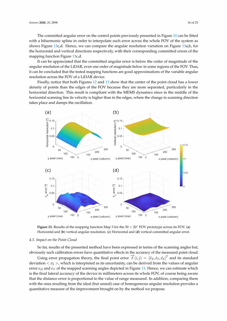
The committed angular error on the control points previously presented in Figure 10 can be fittedwith a biharmonic spline in order to interpolate such error across the whole FOV of the system asshows Figure 13c,d. Hence, we can compare the angular resolution variation on Figure 13a,b, forthe horizontal and vertical directions respectively, with their corresponding committed errors of themapping function Figure 13c,d.

It can be appreciated that the committed angular error is below the order of magnitude of theangular resolution of the LiDAR, even one order of magnitude below in some regions of the FOV. Thus,it can be concluded that the tested mapping functions are good approximations of the variable angularresolution across the FOV of a LiDAR device.

Finally, notice that both Figures 12 and 13 show that the center of the point cloud has a lowerdensity of points than the edges of the FOV because they are more separated, particularly in thehorizontal direction. This result is compliant with the MEMS dynamics since in the middle of thehorizontal scanning line its velocity is higher than in the edges, where the change in scanning directiontakes place and damps the oscillation.

Figure 13. Results of the mapping function Map 3 for the 30 × 20 FOV prototype across its FOV. (a)Horizontal and (b) vertical angular resolution. (c) Horizontal and (d) vertical committed angular error.

4.3. Impact on the Point Cloud

So far, results of the presented method have been expressed in terms of the scanning angles but,obviously such calibration errors have quantitative effects in the accuracy of the measured point cloud.

Using error propagation theory, the final point error−→δ (i, j) = [δX , δY, δZ]

T and its standarddeviation < σk >, which is interpreted as its uncertainty, can be derived from the values of angularerror εH and εV of the mapped scanning angles depicted in Figure 13. Hence, we can estimate whichis the final lateral accuracy of the device in millimeters across its whole FOV, of course being awarethat the distance error is proportional to the value of range measured. In addition, comparing themwith the ones resulting from the ideal (but unreal) case of homogeneous angular resolution provides aquantitative measure of the improvement brought on by the method we propose.

Sensors 2020, 20, 2898 17 of 23

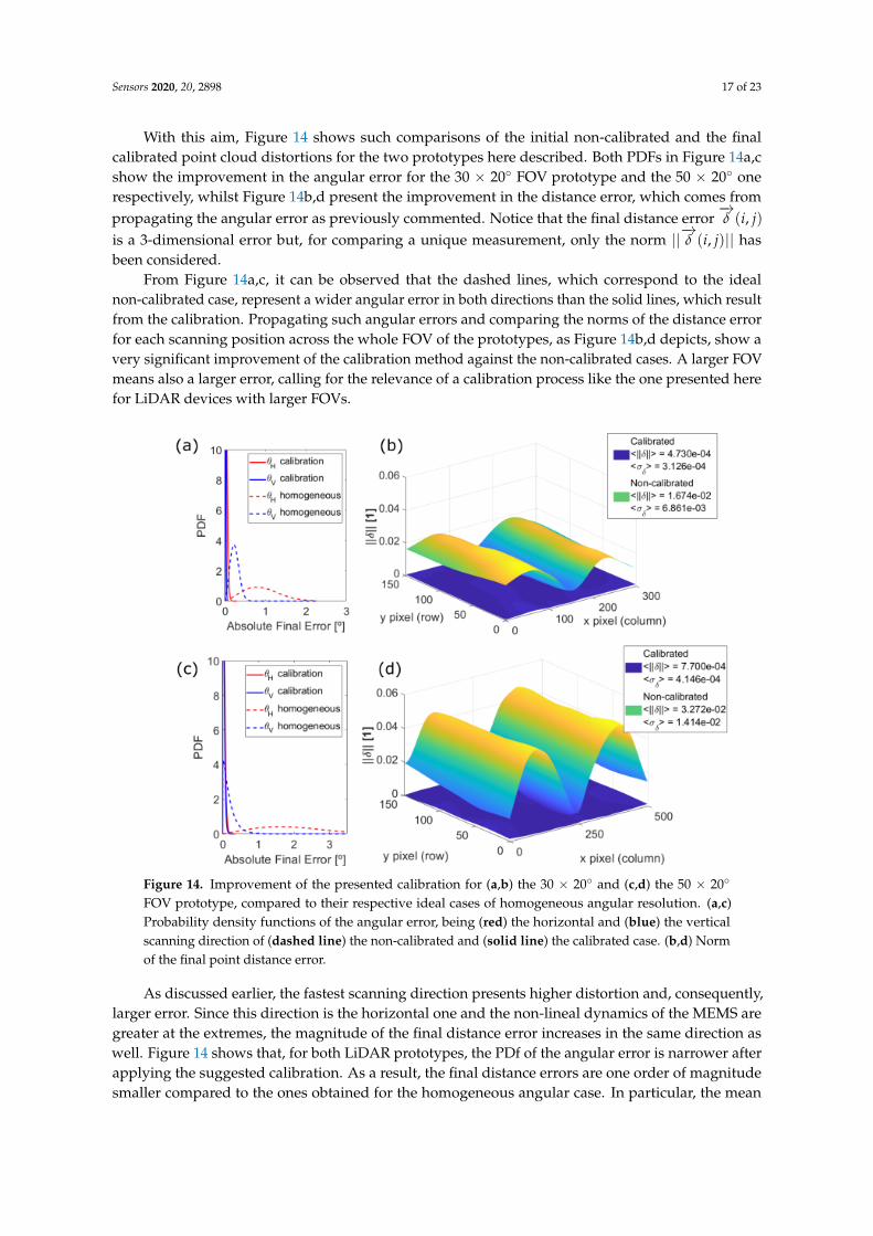
With this aim, Figure 14 shows such comparisons of the initial non-calibrated and the finalcalibrated point cloud distortions for the two prototypes here described. Both PDFs in Figure 14a,cshow the improvement in the angular error for the 30 × 20 FOV prototype and the 50 × 20 onerespectively, whilst Figure 14b,d present the improvement in the distance error, which comes frompropagating the angular error as previously commented. Notice that the final distance error

−→δ (i, j)

is a 3-dimensional error but, for comparing a unique measurement, only the norm ||−→δ (i, j)|| hasbeen considered.

From Figure 14a,c, it can be observed that the dashed lines, which correspond to the idealnon-calibrated case, represent a wider angular error in both directions than the solid lines, which resultfrom the calibration. Propagating such angular errors and comparing the norms of the distance errorfor each scanning position across the whole FOV of the prototypes, as Figure 14b,d depicts, show avery significant improvement of the calibration method against the non-calibrated cases. A larger FOVmeans also a larger error, calling for the relevance of a calibration process like the one presented herefor LiDAR devices with larger FOVs.

Figure 14. Improvement of the presented calibration for (a,b) the 30 × 20 and (c,d) the 50 × 20

FOV prototype, compared to their respective ideal cases of homogeneous angular resolution. (a,c)Probability density functions of the angular error, being (red) the horizontal and (blue) the verticalscanning direction of (dashed line) the non-calibrated and (solid line) the calibrated case. (b,d) Normof the final point distance error.

As discussed earlier, the fastest scanning direction presents higher distortion and, consequently,larger error. Since this direction is the horizontal one and the non-lineal dynamics of the MEMS aregreater at the extremes, the magnitude of the final distance error increases in the same direction aswell. Figure 14 shows that, for both LiDAR prototypes, the PDf of the angular error is narrower afterapplying the suggested calibration. As a result, the final distance errors are one order of magnitudesmaller compared to the ones obtained for the homogeneous angular case. In particular, the mean

Sensors 2020, 20, 2898 18 of 23

value of the error and its uncertainty across the whole FOV are reduced by a factor ∼1/40 and ∼1/30,respectively.

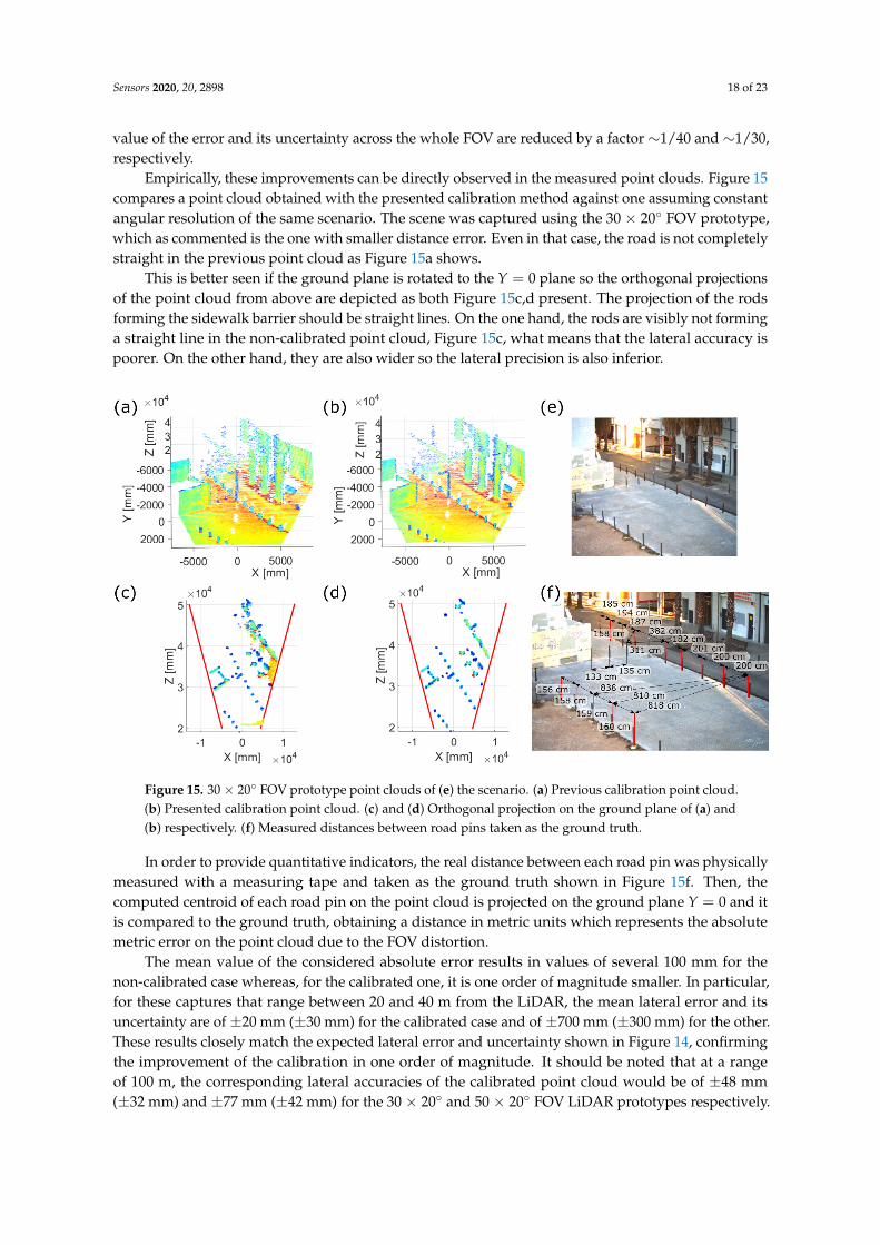
Empirically, these improvements can be directly observed in the measured point clouds. Figure 15compares a point cloud obtained with the presented calibration method against one assuming constantangular resolution of the same scenario. The scene was captured using the 30 × 20 FOV prototype,which as commented is the one with smaller distance error. Even in that case, the road is not completelystraight in the previous point cloud as Figure 15a shows.

This is better seen if the ground plane is rotated to the Y = 0 plane so the orthogonal projectionsof the point cloud from above are depicted as both Figure 15c,d present. The projection of the rodsforming the sidewalk barrier should be straight lines. On the one hand, the rods are visibly not forminga straight line in the non-calibrated point cloud, Figure 15c, what means that the lateral accuracy ispoorer. On the other hand, they are also wider so the lateral precision is also inferior.

Figure 15. 30× 20 FOV prototype point clouds of (e) the scenario. (a) Previous calibration point cloud.(b) Presented calibration point cloud. (c) and (d) Orthogonal projection on the ground plane of (a) and(b) respectively. (f) Measured distances between road pins taken as the ground truth.

In order to provide quantitative indicators, the real distance between each road pin was physicallymeasured with a measuring tape and taken as the ground truth shown in Figure 15f. Then, thecomputed centroid of each road pin on the point cloud is projected on the ground plane Y = 0 and itis compared to the ground truth, obtaining a distance in metric units which represents the absolutemetric error on the point cloud due to the FOV distortion.

The mean value of the considered absolute error results in values of several 100 mm for thenon-calibrated case whereas, for the calibrated one, it is one order of magnitude smaller. In particular,for these captures that range between 20 and 40 m from the LiDAR, the mean lateral error and itsuncertainty are of ±20 mm (±30 mm) for the calibrated case and of ±700 mm (±300 mm) for the other.These results closely match the expected lateral error and uncertainty shown in Figure 14, confirmingthe improvement of the calibration in one order of magnitude. It should be noted that at a rangeof 100 m, the corresponding lateral accuracies of the calibrated point cloud would be of ±48 mm(±32 mm) and ±77 mm (±42 mm) for the 30 × 20 and 50 × 20 FOV LiDAR prototypes respectively.

Sensors 2020, 20, 2898 19 of 23

5. Conclusions

We have introduced a geometrical model for the scanning system of a LiDAR device based onlyin Snell’s law and its specific mechanics, what allows using the same procedure for other scanningtechniques, either solid-state based or mechanical ones, as long as its scanning principle is carefullydescribed. For instance, solid-state LiDAR systems based on Optical Phased Array devices (OPA)can relate their electrical control signals such as frequency with the final scanning direction using thepresented approach.

In particular, for the solid-state MEMS mirror based system analyzed during this work, we haverelated its scanning direction to the tilt angles of the MEMS device, which has been tested to fit withthe performance of a general solid-state LiDAR device including such elements. In addition, such amodel may be used for characterizing the MEMS dynamics, which may be a first step towards eitherclosed-loop control of the mirror oscillation, or, alternatively, towards the correction of the angulardistortion of the optics and the MEMS dynamics by setting appropriate tilt angle dynamics for eachscanning direction of the system.

Furthermore, the suggested geometrical model enables a calibration method which providesan accurate estimation of the varying angular resolution of the scanning system. We would liketo emphasise that this method and the spherical description provided are generic to any scanningtechnique. Consequently, any other LiDAR device can use them and take advantage of their benefits,which are summarized below.

The presented work has been used to improve the accuracy of the measured point clouds, whichwill be more reliable as input for machine learning procedures. In particular, we have shown animprovement of one full order of magnitude in the accuracy of their lateral position measurements,preserving the shape of the objects on the final point cloud. Moreover, considering that the accuracy ofthe mapping functions is below the resolution of the system, other functions might be proposed butsimilar results will be obtained.

Overall, this work provides, for the first time in our knowledge, a general model for LiDARscanning systems based on MEMS mirrors, which provides a simple calibration procedure based onthe measurement of the angular errors of the scanner, which has been confirmed accurate, simple anduseful for the characterization of such devices.

Author Contributions: Investigation, P.G.-G.; Project administration, S.R. and J.R.C.; Software, P.G.-G.;Supervision, S.R., N.R. and J.R.C.; Validation, N.R.; Writing—original draft, P.G.-G., S.R., N.R. and J.R.C. Allauthors have read and agreed to the published version of the manuscript.

Funding: This research was funded by the Ministerio de Ciencia, Innovación y Universidades (MICINN) of Spaingrant number DI-17-09181 and the Agència de Gestió d’Ajuts Universitaris i de Recerca (AGAUR) of Cataloniagrant number 2018-DI-0086.

Acknowledgments: We would like to acknowledge the technical support from Beamagine staff: Jordi Riu,Eduardo Bernal and Isidro Bas; as well as from the UPC: Albert Gil.

Conflicts of Interest: The authors declare no conflict of interest.

Appendix A

In this appendix the reader can find the detailed derivation of some of the key formulas used inprevious sections.

Appendix A.1. Vectorial Snell’s Law

Starting from Equation (2), r = µi + ηn , let us firstly apply the cross-product of the surfacenormal on both sides of the equation.

n× r = µ(n× i) + η(n× n) =⇒ |n| · |r| · sin (θr)A = µ · |n| · |i| · sin (θi)B (A1)

Sensors 2020, 20, 2898 20 of 23

Since all ray vectors lay in the same plane, both A and B are parallel and using the scalar versionof Snell’s law sin θr/ sin θi = ni/nr, the expression for µ is found:

µ =ninr

(A2)

Secondly, let us apply the dot product of the reflected ray with itself in order to find the expressionfor η knowing that θr = −θi so their cosines are equal:

(µi + ηn) · (µi + ηn) = µ2 + η2 + 2µη(n · i) = 1 =⇒ η2 + 2µ(n · i)η + (µ2 − 1) = 0 (A3)

Solving this second order equation, it can be found the final expression for η:

η =−2µ(n · i)±

√4µ2(n · i)2 − 4(µ2 − 1)

2= −µ(n · i)±

√1− µ2(1− (n · i)2) (A4)

Thus, there are two solutions to the above equation: the positive one corresponds to the reflectedcase, while the negative one corresponds to the transmitted case. It can be easily deduced for a raycoming perpendicular onto the surface n = −i, so η = µ± 1 and r = µi + (µ± 1)n = ∓i. Finally,Equation (3) is the result of substituting these expressions for a reflected ray, thus the positive solutionof Equation (A4), in Equation (2).

Appendix A.2. Geometrical Model of MEMS Scanning

As described in Figure 1 in the paper, let us define three reference systems: one for the laser sourceI = i1, i2, i3, another one for the MEMS at its resting or central position M = m1, m2, m3,where m3 = n is coincident with the surface normal at rest; and, finally, one more for the scanningS = s1, s2, s3 where s3 = r, the propagation vector of the beam when the MEMS is at its centralposition too. As it will be shown afterwards, this is the M reference system rotated again, matchings3 with the specular reflection of the incident ray. The aim is to express the MEMS normal and itsincident ray in the same reference system in any scanning case so the set of scanning directions can befound by applying Equation (3).

Let us assume that I is in the origin of the Cartesian coordinate system, as depicted in Figure 1(a) and that the incident laser beam is emitted in the z direction i = z = i3. Additionally, the MEMSdevice is facing towards the laser source but tilted a certain angle ψ in the x-axis. Consequently, usingthe right-hand rule whilst setting m1 = i1 = x, this rotation can be expressed as:

Rx(ψ) =

1 0 00 cos (π + ψ) − sin (π + ψ)

0 sin (π + ψ) cos (π + ψ)

=

1 0 00 − cos (ψ) sin (ψ)

0 − sin (ψ) − cos (ψ)

(A5)

Consequently, the linear transformation from the MEMS reference system M to the source oneI, without taking into account translations because the aim is to obtain its direction, is:

M→IT = Rx(ψ) · Mu (A6)

The driven tilts of the MEMS can be performed about both m1 and m2 MEMS axis. Let us defineα as the angular tilt provoking an horizontal displacement in the FOV whereas β causes a vertical one.Hence, an α counterclockwise rotation can be expressed as a rotation about m2 whilst β about m1.

Sensors 2020, 20, 2898 21 of 23

Rm2(α) ≡ Rα =

cos (α) 0 sin (α)

0 1 0− sin (α) 0 cos (α)

and Rm1(β) ≡ Rβ =

1 0 00 cos (β) − sin (β)

0 sin (β) cos (β)

(A7)

With these rotation matrices, the MEMS surface normal in the laser reference system is defined asthe result of applying β-α-ψ rotations, what defines the first rotation to be taken in the slow directionand matches a proper Euler angle rotation definition x-y-x in the fixed frame M:

In = Rψ · Rα · Rβ · Mn ≡ M→IT(α, β, ψ) · Mn (A8)

As previously commented, the MEMS surface normal in its own reference system M coincideswith the third vector of the basis m3 at the central position. Thus, the final expression for the MEMSnormal in the reference system of the laser source I depending on the tilt angles results in:

In(α, β, ψ) = M→IT(α, β, ψ) ·

001

=

sin (α) cos (β)

cos (ψ) sin (β) + sin (ψ) cos (α) cos (β)

sin (ψ) sin (β)− cos (ψ) cos (α) cos (β)

(A9)

Notice that if the small angle approximation is assumed for all angles (cos (x) ∼ 1 and sin (x) ∼ x),rotations are commutative because any rotation order leads to In = [α, β + ψ, βψ− 1]T .

Now that both vectors, the MEMS normal and the incident ray, are expressed in the same referencesystem, the expression for the scanning direction depending on the tilt angles can be found. Firstly, letus define γ(α, β, ψ) as the dot product between the MEMS normal and the incident ray.

γ(α, β, ψ) ≡(InT ·I i

)=

sin (α) cos (β)

cos (ψ) sin (β) + sin (ψ) cos (α) cos (β)

sin (ψ) sin (β)− cos (ψ) cos (α) cos (β)

T

·

001

=

= sin (ψ) sin (β)− cos (ψ) cos (α) cos (β)

(A10)

I s = I i−(

γ(α, β, ψ)−√

γ(α, β, ψ)2)In (A11)

In particular, as previously commented, when the MEMS is at its rest position with α = β = 0,the reflected ray results in:

I s(0, 0, ψ) =

001

−(− cos (ψ)−√(− cos (ψ))2

) 0sin (ψ)

− cos (ψ)

=

02 cos (ψ) sin (ψ)

1− 2 cos (ψ)2

=

0sin (2ψ)

− cos (2ψ)

(A12)

Which is exactly the specular reflection of the incident ray with angle 2ψ. To sum up, let us write downthe defined set of basis being aware that there is a translation with respect from the laser source andthat they are defined for α = β = 0.

I = i, j, k, M =

i,−

0cos (ψ)sin (ψ)

,

0sin (ψ)

− cos (ψ)

and S =

i,−

0cos (2ψ)

sin (2ψ)

,

0sin (2ψ)

− cos (2ψ)

(A13)

Thus, this is the set of reference basis that characterize the scanning of a LiDAR system.

Sensors 2020, 20, 2898 22 of 23

References

1. Fernald, F.G. Analysis of atmospheric lidar observations: Some comments. Appl. Opt. AO 1984, 23, 652.[CrossRef] [PubMed]

2. Korb, C.L.; Gentry, B.M.; Weng, C.Y. Edge technique: Theory and application to the lidar measurement ofatmospheric wind. Appl. Opt. 1992, 31, 4202–4213. [CrossRef] [PubMed]

3. McGill, M.J. Lidar Remote Sensing. In Encyclopedia of Optical Engineering; Marcel Dekker: New York, NY,USA, 2003; pp. 1103–1113.

4. Liu, X. Airborne LiDAR for DEM generation: Some critical issues. Prog. Phys. Geogr. Earth Environ. 2008,32, 31–49. [CrossRef]

5. Mallet, C.; Bretar, F. Full-waveform topographic lidar: State-of-the-art. ISPRS J. Photogramm. Remote Sens.2009, 64, 1–16. [CrossRef]

6. Azuma, R.T.; Malibu, I. A Survey of Augmented Reality. Presence Teleoperators Virtual Environ. 1997,6, 355–385. [CrossRef]

7. Azuma, R.; Baillot, Y.; Behringer, R.; Feiner, S.; Julier, S.; MacIntyre, B. Recent advances in augmentedreality. IEEE Comput. Graph. Appl. 2001, 21, 34–47. [CrossRef]

8. Schwarz, B. LIDAR: Mapping the world in 3D. Nat. Photonics 2010, 4, 429–430. [CrossRef]9. Royo, S.; Ballesta-Garcia, M. An Overview of Lidar Imaging Systems for Autonomous Vehicles. Appl. Sci.

2019, 9, 4093. [CrossRef]10. Takagi, K.; Morikawa, K.; Ogawa, T.; Saburi, M. Road Environment Recognition Using On-vehicle LIDAR.

In Proceedings of the 2006 IEEE Intelligent Vehicles Symposium, Tokyo, Japan, 13–15 June 2006; pp.120–125. [CrossRef]

11. Premebida, C.; Monteiro, G.; Nunes, U.; Peixoto, P. A Lidar and Vision-based Approach for Pedestrianand Vehicle Detection and Tracking. In Proceedings of the 2007 IEEE Intelligent Transportation SystemsConference, Seattle, WA, USA, 30 September–3 October 2007; pp. 1044–1049. [CrossRef]

12. Gallant, M.J.; Marshall, J.A. The LiDAR compass: Extremely lightweight heading estimation with axismaps. Robot. Auton. Syst. 2016, 82, 35–45. [CrossRef]

13. Huynh, D.Q.; Owens, R.A.; Hartmann, P.E. Calibrating a Structured Light Stripe System: A NovelApproach. Int. J. Comput. Vis. 1999, 33, 73–86. [CrossRef]

14. Glennie, C.; Lichti, D.D. Static Calibration and Analysis of the Velodyne HDL-64E S2 for High AccuracyMobile Scanning. Remote Sens. 2010, 2, 1610–1624. [CrossRef]

15. Muhammad, N.; Lacroix, S. Calibration of a rotating multi-beam lidar. In Proceedings of the 2010IEEE/RSJ International Conference on Intelligent Robots and Systems, Taipei, Taiwan, 18–22 October 2010;pp. 5648–5653. [CrossRef]

16. Atanacio-Jiménez, G.; González-Barbosa, J.J.; Hurtado-Ramos, J.B.; Ornelas-Rodríguez, F.J.;Jiménez-Hernández, H.; García-Ramirez, T.; González-Barbosa, R. LIDAR Velodyne HDL-64E CalibrationUsing Pattern Planes. Int. J. Adv. Robot. Syst. 2011, 8, 59. [CrossRef]

17. Mirzaei, F.M.; Kottas, D.G.; Roumeliotis, S.I. 3D LIDAR–camera intrinsic and extrinsic calibration:Identifiability and analytical least-squares-based initialization. Int. J. Robot. Res. 2012, 31, 452–467.[CrossRef]

18. Yu, C.; Chen, X.; Xi, J. Modeling and Calibration of a Novel One-Mirror Galvanometric Laser Scanner.Sensors 2017, 17, 164. [CrossRef] [PubMed]

19. Cui, S.; Zhu, X.; Wang, W.; Xie, Y. Calibration of a laser galvanometric scanning system by adapting acamera model. Appl. Opt. AO 2009, 48, 2632–2637. [CrossRef]

20. Rodriguez, F.S.A.; Fremont, V.; Bonnifait, P. Extrinsic calibration between a multi-layer lidar and a camera.In Proceedings of the 2008 IEEE International Conference on Multisensor Fusion and Integration forIntelligent Systems, Seoul, Korea, 20–22 August 2008; pp. 214–219. [CrossRef]

21. Kwak, K.; Huber, D.F.; Badino, H.; Kanade, T. Extrinsic calibration of a single line scanning lidar and acamera. In Proceedings of the 2011 IEEE/RSJ International Conference on Intelligent Robots and Systems,San Francisco, CA, USA, 25–30 September 2011; pp. 3283–3289.

22. Zhou, L.; Deng, Z. Extrinsic calibration of a camera and a lidar based on decoupling the rotation from thetranslation. In Proceedings of the 2012 IEEE Intelligent Vehicles Symposium, Alcala de Henares, Spain, 3–7June 2012; pp. 642–648. [CrossRef]

Sensors 2020, 20, 2898 23 of 23

23. García-Moreno, A.I.; Gonzalez-Barbosa, J.J.; Ornelas-Rodriguez, F.J.; Hurtado-Ramos, J.B.; Primo-Fuentes,M.N. LIDAR and Panoramic Camera Extrinsic Calibration Approach Using a Pattern Plane. In PatternRecognition; Hutchison, D., Kanade, T., Kittler, J., Kleinberg, J.M., Mattern, F., Mitchell, J.C., Naor, M.,Nierstrasz, O., Pandu Rangan, C., Steffen, B., et al., Eds.; Springer: Berlin/Heidelberg, Germany, 2013;Volume 7914, pp. 104–113. [CrossRef]

24. Park, Y.; Yun, S.; Won, C.S.; Cho, K.; Um, K.; Sim, S. Calibration between Color Camera and 3D LIDARInstruments with a Polygonal Planar Board. Sensors 2014, 14, 5333–5353. [CrossRef]

25. Dhall, A.; Chelani, K.; Radhakrishnan, V.; Krishna, K.M. LiDAR-Camera Calibration using 3D-3D Pointcorrespondences. arXiv 2017, arXiv:1705.09785.

26. Guindel, C.; Beltrán, J.; Martín, D.; García, F. Automatic extrinsic calibration for lidar-stereo vehicle sensorsetups. In Proceedings of the 2017 IEEE 20th International Conference on Intelligent TransportationSystems (ITSC), Yokohama, Japan, 16–19 October 2017; pp. 1–6. [CrossRef]

27. Urey, H.; Holmstrom, S.; Baran, U. MEMS laser scanners: A review. J. Microelectromech. Syst. 2014, 23, 259.[CrossRef]

28. Ortiz, S.; Siedlecki, D.; Grulkowski, I.; Remon, L.; Pascual, D.; Wojtkowski, M.; Marcos, S. Optical distortioncorrection in Optical Coherence Tomography for quantitative ocular anterior segment by three-dimensionalimaging. Opt. Express OE 2010, 18, 2782–2796. [CrossRef]

29. Brown, D.C. Decentering Distortion of Lenses. Photogramm. Eng. 1966, 32, 444–462.30. Swaninathan, R.; Grossberg, M.D.; Nayar, S.K. A perspective on distortions. In Proceedings of the 2003

IEEE Computer Society Conference on Computer Vision and Pattern Recognition, Madison, WI, USA,18–20 June 2003; Volume 2. [CrossRef]

31. Pan, B.; Yu, L.; Wu, D.; Tang, L. Systematic errors in two-dimensional digital image correlation due to lensdistortion. Opt. Lasers Eng. 2013, 51, 140–147. [CrossRef]

32. Bauer, A.; Vo, S.; Parkins, K.; Rodriguez, F.; Cakmakci, O.; Rolland, J.P. Computational optical distortioncorrection using a radial basis function-based mapping method. Opt. Express OE 2012, 20, 14906–14920.[CrossRef] [PubMed]

33. Li, A.; Wu, Y.; Xia, X.; Huang, Y.; Feng, C.; Zheng, Z. Computational method for correcting complex opticaldistortion based on FOV division. Appl. Opt. AO 2015, 54, 2441–2449. [CrossRef] [PubMed]

34. Sun, C.; Guo, X.; Wang, P.; Zhang, B. Computational optical distortion correction based on local polynomialby inverse model. Optik 2017, 132, 388–400. [CrossRef]

35. Heikkila, J.; Silven, O. A four-step camera calibration procedure with implicit image correction.In Proceedings of the IEEE Computer Society Conference on Computer Vision and Pattern Recognition,San Juan, Puerto Rico, 17–19 June 1997; pp. 1106–1112. [CrossRef]

c© 2020 by the authors. Licensee MDPI, Basel, Switzerland. This article is an open accessarticle distributed under the terms and conditions of the Creative Commons Attribution(CC BY) license (http://creativecommons.org/licenses/by/4.0/).