Soil surface resistance to runoff

Researching the resistance of different soil surfaces and post-harvest tillage types to flow

MSc. Thesis (minor)

Ton van der Linden

Wageningen University,

Soil Physics and Land Management Group

The Netherlands

Bioforsk, Norwegian Institute for Agricultural and Environmental Research

Soil and Environment Department

Norway

May 2015

ii

Soil surface resistance to

runoff

Researching the resistance of different soil surfaces

and post-harvest tillage types to flow

MSc. Thesis (minor)

Ton van der Linden

Wageningen University,

Soil Physics and Land Management Group

The Netherlands

Supervision: ir. Jantiene Baartman & dr. Jerry Maroulis

Bioforsk –Soil and Environment–,

Norwegian Institute for Agricultural and Environmental Research

Norway

Supervision: dr. Jannes Stolte

May 2015

Wageningen, The Netherlands

iii

ABSTRACT This thesis explored the influence of soil surface resistance (Manning’s n) to runoff and soil

erosion by inserting new data into the LISEM erosion model for the Gryteland catchment near

Ås, southeast Norway. Fieldwork was undertaken to measure Manning’s n. Measurements were

carried out for five land units based on soil type, land use, crop and tillage. LISEM was used to

research the effect of soil surface resistance on runoff leaving the catchment by comparing the

hydrographs of model runs using the original, literature-based Manning’s n input data and the

new, field-measured data. Three rainfall events, having different intensities and duration, were

applied in the model runs. Results showed an increased runoff due to lower (onsite measured)

Manning’s n values during the rainfall events. During the runs, these larger runoff amounts

levelled out until the level of computed runoff for original Manning’s n values, indicating the

disappearance of Manning’s n effect. An assessment of tillage types on erosion reduction was

carried out. Tilled soil, cultivated by means of a chisel plow, appeared to be the best solution

regarding computed soil loss during low intensity rainfall events, while this scenario is the worst

case during high intensity rainfall events. Constructing grass strips in waterways is the best soil

conservation solution; a reduction in soil loss of about 50% was computed relative to that of

tilled soil. Tillage or zero tillage at higher ends of the field does not make a difference in this

case. Taking into account future changes such as climate change, introducing grass strips in the

waterways is recommended.

Key words: Manning’s n, soil surface resistance, erosion, Limburg soil erosion model, tillage, rainfall

intensity, runoff, soil loss

iv

ACKNOWLEDGEMENT This thesis has been submitted as part of the Master of Science International Land and Water

Management at Wageningen UR.

I want to thank my supervisor Jannes Stolte for giving me the opportunity to carry out this

research and for his help and advice. I also want to thank Jantiene Baartman and Jerry Maroulis

for their supervision and useful feedback. Thanks to Robert Barneveld and his family, Johannes

Deelstra, Csilla Farkas, Alice Budai, Inga Greipsland and Torsten Starkloff for their advice and

commitment during my stay in Ås. Further, I want to thank my family for their support during

and after my stay in Norway.

Wageningen, May 2015

Ton van der Linden

v

TABLE OF CONTENTS Abstract ................................................................................................................................................................................ iii

Acknowledgement ............................................................................................................................................................iv

List of appendices ........................................................................................................................................................... vii

List of tables ...................................................................................................................................................................... vii

List of figures .................................................................................................................................................................... vii

1. Introduction ................................................................................................................................................................ 1

1.1 Introduction to soil erosion processes and modelling ........................................................................... 1

1.2 Problem statement ................................................................................................................................................ 2

1.3 Objectives .................................................................................................................................................................. 2

1.4 Research questions ............................................................................................................................................... 2

1.5 Report Outline ......................................................................................................................................................... 2

2. Study area .................................................................................................................................................................... 3

3. Methodology ............................................................................................................................................................... 5

3.1 Land units ................................................................................................................................................................. 5

3.2 Manning’s n .............................................................................................................................................................. 6

3.3 LISEM .......................................................................................................................................................................... 7

3.3.1 Model explanation......................................................................................................................................... 7

3.3.2 Rainfall events ................................................................................................................................................ 8

3.3.3 Calibration ........................................................................................................................................................ 9

3.4 Tillage assessment................................................................................................................................................. 9

4. Results ........................................................................................................................................................................ 11

4.1 Field measurement outcomes ....................................................................................................................... 11

4.2 Manning’s n effect in LISEM modelling ...................................................................................................... 13

4.2.1 Mapping Manning’s n values ................................................................................................................. 13

4.2.2 Model calibration ....................................................................................................................................... 13

4.2.3 Manning’s n effect on other rainfall events ..................................................................................... 14

4.3 Tillage assessment.............................................................................................................................................. 15

4.3.1 Scenario 1: Tilled soil ................................................................................................................................ 15

4.3.2 Scenario 2: Zero tillage ............................................................................................................................. 16

4.3.3 Scenario 3: Tilled soil with grass strips in waterways ................................................................ 17

4.3.4 Scenario 4: Untilled soil with grass strips in waterways ........................................................... 19

5. Discussion ................................................................................................................................................................. 21

5.1 Manning’s n effect in LISEM modelling ...................................................................................................... 21

5.2 Tillage effects on soil loss and total runoff ............................................................................................... 23

vi

5.3 Recommendations .............................................................................................................................................. 24

5.4 Research limitations and future research ................................................................................................ 25

6. Conclusion ................................................................................................................................................................ 26

References .......................................................................................................................................................................... 27

Appendices ........................................................................................................................................................................ 29

vii

LIST OF APPENDICES Appendix 1 Selection of LISEM input map p. 30

Appendix 2 Field measurement results p. 31

Appendix 3 Box plot analysis p. 43

Appendix 4 T-test analysis p. 45

LIST OF TABLES Table 1: Average Manning's n values per land unit. p. 12

Table 2: Comparison of soil loss and total runoff for the tilled soil and tilled soil p. 16

combined with zero tillage of the waterways.

Table 3: Comparison of soil loss and total runoff for the tilled soil zero tillage. p. 17

Table 4: Results of model runs showing the soil loss (kg/ha) and total runoff (m3) for p. 18

tilled soil and tilled soil combined with Grass strips in the waterways.

Table 5: Results of model runs showing the soil loss (kg/ha) and total runoff (m3) for p. 20

tilled soil and zero tillage combined with grass strips in the waterways.

Table 6: Soil loss and Total discharge compared with tilled soil in percentages. p. 24

LIST OF FIGURES Figure 1: Southern Norway and the location of the Skuterud catchment. p. 3

Figure 2: Skuterud catchment, in colour the Gryteland sub-catchment p. 3

Figure 3: View of the Gryteland sub-catchment after harvest. This picture shows the p. 3

post-harvest conditions of 2014: tilled field and the untilled waterways.

Figure 4: Tilled soil by chisel plow. p. 4

Figure 5: Wheat stubble on zero tilled soil. p. 4

Figure 6: Perennial grass. p. 4

Figure 7: Land unit determination based on soil type, land use, crop and tillage. p. 5

The green boxes are the land units where measurements were carried out.

The grey boxes were selected, no measurements were carried out.

Figure 8: The measurement set up showing the plot bounded by two small walls, p. 6

the Mariotte bottles, the flume and bucket.

Figure 9: Scheme of physical processes in LISEM. p. 8

Figure 10: Rainfall events used for LISEM expressed as rainfall intensities (mm/h). p. 9

Figure 11: The Adjusted rr-map (post-harvest conditions 2014): Tilled soil 1.63, p. 10

Zero tillage 1.24, Forest 1.07.

Figure 12: The Original rr-map: Arable land: 0.88, forest 3.2. p. 10

Figure 13: Post-harvest field conditions 2014: chisel plow tilled soil combined with p. 10

zero tillage in the waterways.

Figure 14: Soil map of the Skuterud catchment, showing the area location of the p. 11

Gryteland sub-catchment.

Figure 15: Plot locations within Gryteland represented on land use map in PCRaster. p. 11

Figure 16: Boxplot of Manning’s ns of five plots showing the deviations and the mutual p. 12

differences.

Figure 17: Original Manning's n-map: arable land: 0.25, forest 1.2. p. 13

Figure 18: Adjusted Manning's n map based on field measurements. p. 13

Figure 19: Hydrograph of the Measured Runoff discharge, uncalibrated and calibrated p. 13

model runs including the original n-map and the adjusted n-map. The calibrated

runs have equal multiplications of Ksat (5.5).

Figure 20: Modelling results for rainfall event of 29 August 2011 showing a higher runoff p. 14

viii

intensity peak for the run with adjusted Manning’s n values.

Figure 21: Modelling results of rainfall event of 19 August 2008 showing minor differences p. 14

of the runs.

Figure 22: Hydrograph comparison of tilled soil versus tilled soil combined with zero tillage p. 15

of the waterways, rainfall event 29 August 2008.

Figure 23: Hydrograph comparison of the tilled soil versus tilled soil combined with p. 15

zero tillage.

of the waterways, rainfall event 13 August 2010.

Figure 24: Hydrograph comparison of tilled soil versus zero tillage for the rainfall event p. 16

on 29 August 2008.

Figure 25: Hydrograph comparison of tilled soil versus zero tillage for the rainfall event on p. 17

13 August 2010.

Figure 26: Hydrograph comparison of tilled soil versus tilled soil combined with grass strips p. 18

in the waterways for the rainfall event on 29 August 2008.

Figure 27: Hydrograph comparison of tilled soil versus tilled soil combined with grass strips p. 18

in the waterways for the rainfall event on 13 August 2010.

Figure 28: Hydrograph comparison of tilled soil versus zero tillage combined with p. 19

grass strips in the waterways for the rainfall event on 29 August 2008.

Figure 29: Hydrograph comparison of tilled soil versus zero tillage combined with p. 19

grass strips in the waterways for the rainfall event on 13 August 2010.

Figure 30: List of Manning’s n values from the literature. p. 20

Figure 31: Relationship Manning’s n and slope angle (Hessel et al., 2003). p. 22

Figure 32: Digital elevation model (meters above sea level). p. 30

Figure 33: Soil profiles, 102: forest on clay, 103: cropland on clay, 202: forest on sand, p. 30

203: cropland on sand.

Figure 34: Aggregate stability (-/-): 200. p. 30

Figure 35: Stone fraction (-/-): 0. p. 30

Figure 36: Cohesion (kPa), arable land: 0.25, Forest: 500. p. 30

Figure 37: Cohesion by roots (kPa), arable land: 1, forest: 10. p. 30

Figure 38: Crust fraction (-/-): 0. p. 31

Figure 39: Vegetation height (m), arable land: 0.7, forest: 7. p. 31

Figure 40: Compaction fraction (-/-): 0. p. 31

Figure 41: Leaf area index (-/-), arable land: 2.5, forest 6. p. 31

Figure 42: Saturated hydraulic conductivity (mm/h), arable land: 1.69, forest 1.66, p. 31

garden 0.69.

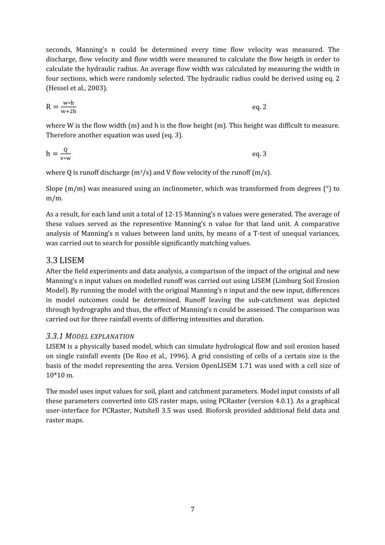
Figure 43: Representation of zero tillage on clay loam soil. p. 32

Figure 44: Representation of tilled clay loam soil. p. 34

Figure 45: Representation of the grass surface. p. 37

Figure 46: Representation of tilled sandy silt soil. p. 39

Figure 47: Representation of zero tillage on sandy silt soil. p. 42

Figure 48: Boxplot of Manning's n values showing the deviations for each land unit. p. 45

1. INTRODUCTION

1.1 INTRODUCTION TO SOIL EROSION PROCESSES AND MODELLING Agriculture and sustainable land use can be difficult to combine. Land degradation, the loss of

soil functions, is a result of natural processes, but mostly it is human induced or accelerated by

human impact (Imeson, 2011). Degradation of land has many causes, ranging from depletion of

ground water resources to the use of pesticides for agricultural purposes.

Soil erosion is an environment changing process, which is a form of land degradation. This

process occurs everywhere around the world. Besides arid and semi-arid regions, regions with

milder climate conditions also face soil erosion problems. In these regions, the agricultural

sector has undergone a process of intensification, resulting in higher production rates.

Monocultures and intensive tillage are examples of this development.

Soil cultivation can lead to increased soil erosion (Morgan, 2005; Zachar, 1982). The lack of soil

cover in autumn and winter and the removal of natural obstacles (i.e. forests and rocks) in fields

result in less infiltration and water retention, which generates runoff. Runoff causes detachment

and distribution of soil particles and finally the sedimentation of these particles. In general, the

top soil loses fertility since it contains nutrients and organic matter that will be removed by

erosion. In the long term this can negatively affect plant growth and so agricultural productivity

will decline (Morgan, 2005).

The extent of the erosion problem indicates the urgency for sustainable land management in

these intensively used agricultural fields (Zachar, 1982). The spatial and temporal variation of

the environment should be investigated to get more understanding of the erosion rates (Morgan,

2005). Since the early nineties of the last century, several erosion models have been developed

to be able to estimate these erosion rates (Smith et al., 2010). These models calculate and

visualize environmental changes; changes in the past can be explained, and effects of future

scenarios can be simulated. However, developing an accurate model is difficult, caused by the

spatial variability and accuracy of input parameters (De Vente et al., 2013).

Calculation of flow velocity to simulate the flow of water over the land surface is a basic need in

hydrological and soil erosion models. Overland flow can be calculated by two equations: the

Darcy-Weisbach equation and Manning’s equation. Both equations contain a factor representing

soil resistance to water flow. Abrahams et al. (1990) studied Darcy-Weisbach resistance factor

(f) and found that it varies with flow rate, meaning that f is highly variable in space and time, as

it depends on continuously changing flow conditions. This dependency is related to Reynolds

number and Chezy C (Abrahams et al., 1990; Emmett, 1970). Hessel et al. (2003) found that

Manning’s n behaves in the same way as f (Darcy-Weisbach), and can be estimated from

Reynolds number too. Manning’s n was found to increase with slope angle, caused by a hardly

increasing flow velocity with increasing slope, implying that in soil erosion models, the value of

n should be a function of slope for surfaces that can erode by runoff.

Manning’s n appeared to be an important parameter in erosion modelling, however, Manning’s n

values used for erosion modelling assignments are usually based on literature data; onsite

measurements of these values are rare. Only few studies have been carried out where onsite

measured Manning’s n values are used. The question arises how the modelling results are

2

affected by Manning’s n parameter values; it indicates the need for carrying out onsite

measurements.

More knowledge on soil resistance to water flow can contribute to studies where soil

conservation measures and tillage practices are assessed. There has been considerable debates

for years about the soil cultivation effects on erosion after harvest as to whether it increases or

decreases erosion rates. This study could contribute to a new approach in combating soil

erosion in these intensively used agricultural fields in eastern Norway.

1.2 PROBLEM STATEMENT In the case of erosion modelling, creating an accurate representation of the real situation is

challenging (Jetten et al., 2003). If input data cannot be collected by field measurements, these

are mainly based on values taken from the literature, or generated using e.g. pedotransfer

functions.

The Limburg Soil Erosion Model (LISEM) has been used to calculate erosion rates for the

Gryteland sub-catchment, part of the Skuterud catchment near Ås in southeast Norway (Kværno

and Stolte, 2012). In this study, the initial Manning’s n values were based on literature data. As a

result, the correctness of these values and the influence on the model outcomes are unknown,

while the sensitivity of Manning’s n for calculating the erosion rates is high (De Roo et al., 1994).

1.3 OBJECTIVES The main objective of this research was to obtain onsite-measured values for Manning’s n for

identified land units as input for the LISEM soil erosion model. The second objective was to

compare the model outputs using these field-measured Manning’s n values and literature-

derived Manning’s n values. Finally, an assessment of the effect of tillage practices on erosion

was carried out using LISEM.

1.4 RESEARCH QUESTIONS The main research questions were:

How do computed LISEM outputs for the Gryteland sub-catchment change when using

onsite measured Manning’s n values in comparison with using Manning’s n values derived

from literature?

Which tillage practices are most effective in erosion reduction for the Gryteland sub-

catchment?

1.5 REPORT OUTLINE This report will go through several steps resulting in answering the research questions. A

separate section is spent on the study area, chapter 2. Chapter 3 contains the methodology,

followed by chapter 4 providing the results of the field experiments, the modelling outcomes,

and the assessment of different tillage types on erosion. Discussion and further research are

presented in chapter 5. In chapter 6, the conclusions are provided, containing the main findings

of the research.

3

2. STUDY AREA This research was carried out in the Skuterud catchment in Akershus County, located in the

southeast of Norway (Fig. 1). The catchment is part of the JOVA program, which is a land use and

water-monitoring program in Norwegian agricultural catchments. This program was started in

1992 with the aim to investigate the effects of agricultural practices on water quality and soil

condition (Bioforsk, 2014).

The catchment size is approximately 450 ha which mostly consists of arable land (60%),

surrounded by forest (33%). A small part of the forest consists of peat land. The eastern part of

the catchment is urban area (7%). The soils in the centre of the catchment consist of marine

sediments; silt loam and clay loam containing gravel and stones, classified as Albeluvisols and

Stagnosols. Surrounding the marine deposits, sandy silt and loamy sands are present, classified

as Cambisols, Arenosols, Umbrisols, Podzols and Gleysols. In the higher parts of the catchment

deposits consist of coarser materials. The catchment is split by marginal moraine ridges coming

from the ice cap melting at the end of the last glacial period (Kværno and Stolte, 2012).

The mean annual temperature is 5.3°C and mean precipitation is 785 mm per year. The

topography has a rolling character with altitudes ranging from 92 to 150m above sea level.

Slopes range from 0° in the middle of the catchment to 30° at the edges of the catchment

(Kværno and Stolte, 2012).

The main crops are cereals, which are sometimes rotated with cover crops in winter (in the case

of spring-sown cereals). Grass strips of approximately 5m width are present adjacent to the

stream.

In a sub-catchment, Gryteland (27 ha) (Figs. 2 and 3), drainage water and runoff water are

monitored separately. For LISEM modelling, this partition of hydrological processes is a major

advantage, which made the area suitable to carry out this research for Manning’s n. In previous

years measurements on several other input parameters of LISEM have been carried out in this

area, such as aggregate stability and random roughness (Kværno and Stolte, 2012; Thomsen,

2013).

FIGURE 1: SOUTHERN NORWAY

AND THE LOCATION OF THE

SKUTERUD CATCHMENT

(GOOGLE.MAPS, 2014).

FIGURE 2: SKUTERUD

CATCHMENT, IN COLOUR THE

GRYTELAND SUB-CATCHMENT.

FIGURE 3: VIEW OF THE GRYTELAND SUB-CATCHMENT AFTER

HARVEST 2014. THIS PICTURE SHOWS THE POST-HARVEST

CONDITION OF AUTUMN 2014: TILLED FIELD AND THE UNTILLED

WATERWAYS.

4

FIGURE 4: TILLED SOIL BY CHISEL PLOW.

FIGURE 5: WHEAT STUBBLE ON UNTILLED SOIL.

FIGURE 6: PERENNIAL GRASS.

The emphasis of this research is on arable

land. Tillage practices are determinants for

runoff and erosion. Three post-harvest tillage

practices were observed in the Gryteland

catchment. The first type of soil tillage is

cultivation by a chisel plow. Stubble was

mixed with the soil, resulting in a loosened soil

and a soil cover of approximately 20%-30%

(Fig. 4).

Zero tillage is a practice where arable field is

untreated after harvest. The soil is not

loosened and soil cover consists of wheat

stubble, covering about 80%-90%. Tracks of

machinery are still present, resulting in a

compacted top soil (Fig. 5).

Perennial grass has a full vegetation cover.

This grass is used for erosion protection near

the channel and as headland, but it is not used

for cattle feed, resulting in a limited treatment

of mowing at most two times a year (Fig. 6).

5

3. METHODOLOGY

3.1 LAND UNITS Manning’s n depends on surface cover, which spatially differs within the Gryteland sub-

catchment. Land units were established based on a combination of soil type, land use, crop and

tillage practice. According to these land units, measurement locations were determined. The

number of soil types in the Gryteland sub-catchment is limited to sandy silt and clay loam while

other soil types are excluded since their presence is negligible.

Land units have diverse properties, which affect the runoff rate, and probably Manning’s n. The

seasons also influence Manning’s n values through changing vegetation type, density, and soil

tillage. This research was based on post-harvest conditions of 2014.

Fig. 7 shows the selection of land units. This resulted in a selection of eight land units (green and

grey coloured boxes in Fig. 7) where Manning’s n was supposed to be measured. However,

several constraints and simplifications, such as limited accessibility, the number of land units

investigated was reduced to five land units, shown in the green coloured boxes.

Clay loam

Agriculture

Infrastructure

Nature

Wheat

Grass

Untreated

Harrowed

Perennial

Annual

Sandy silt

Agriculture

Infrastructure

Nature

Wheat

Grass

Untreated

Harrowed

Perennial

Annual

Soil type Land use Crop Tillage

FIGURE 7: LAND UNIT DETERMINATION BASED ON SOIL TYPE, LAND USE, CROP AND TILLAG. THE GREEN BOXES

ARE THE LAND UNITS WHERE MEASUREMENTS WERE CARRIED OUT. THE GREY BOXES WERE SELECTED LAND

UNITS BUT NO MEASUREMENTS ARE CARRIED OUT.

6

3.2 MANNING’S N Manning’s n is the indicator of soil resistance to water flow in channels and surface flow

(Tinkler, 1997). This factor depends on surface cover. It is part of the Gauckler-Manning

equation that estimates the velocity of runoff (Jetten, 2002) (eq. 1).

V =k

n∗ R(

2

3) ∗ S(

1

2) eq. 1

where V is flow velocity (m/s), K is a conversion factor, depending on the units of R and S, S is

slope (m/m), and R hydraulic radius (m). The hydraulic radius can be determined by dividing

the cross-sectional area (A) by the wetted perimeter (Pw) R = A/Pw while N, Manning’s n, is a

dimensionless parameter. Manning’s n was derived by measuring flow velocity and the other

parameters of the Gauckler-Manning formula.

Field measurements were based on the set up (Fig. 8) developed by Hessel et al. (2003). To

generate runoff, the top of the surface had to be pre-wetted until saturation. Two Mariotte

bottles on the top of the plot drained water into a smaller bottle which directed the water into a

gutter. This gutter divided water equally over the full width of the plot. Water flowed down over

the surface and exited through a flume and into a bucket. The plot was delineated by two small

walls to regulate the flow. Dye was added at the slide of the gutter to visualize the water flow

and the time was noted when it entered the flume to calculate the flow velocity (distance/time).

The length of the plots varied from 1.5m to 2.5 m.

The measurement per land unit was repeated three times for approximately 10 minutes. For

each run, the flow velocity was measured several times. By measuring discharge every 30

FIGURE 8: THE MEASUREMENT SET UP SHOWING THE PLOT BOUNDED BY TWO SMALL WALLS, THE MARIOTTE

BOTTLES, THE FLUME, AND BUCKET.

7

seconds, Manning’s n could be determined every time flow velocity was measured. The

discharge, flow velocity and flow width were measured to calculate the flow heigth in order to

calculate the hydraulic radius. An average flow width was calculated by measuring the width in

four sections, which were randomly selected. The hydraulic radius could be derived using eq. 2

(Hessel et al., 2003).

R =w∗h

w+2h eq. 2

where W is the flow width (m) and h is the flow height (m). This height was difficult to measure.

Therefore another equation was used (eq. 3).

h =Q

v∗w eq. 3

where Q is runoff discharge (m3/s) and V flow velocity of the runoff (m/s).

Slope (m/m) was measured using an inclinometer, which was transformed from degrees (°) to

m/m.

As a result, for each land unit a total of 12-15 Manning’s n values were generated. The average of

these values served as the representive Manning’s n value for that land unit. A comparative

analysis of Manning’s n values between land units, by means of a T-test of unequal variances,

was carried out to search for possible significantly matching values.

3.3 LISEM After the field experiments and data analysis, a comparison of the impact of the original and new

Manning’s n input values on modelled runoff was carried out using LISEM (Limburg Soil Erosion

Model). By running the model with the original Manning’s n input and the new input, differences

in model outcomes could be determined. Runoff leaving the sub-catchment was depicted

through hydrographs and thus, the effect of Manning’s n could be assessed. The comparison was

carried out for three rainfall events of differing intensities and duration.

3.3.1 MODEL EXPLANATION LISEM is a physically based model, which can simulate hydrological flow and soil erosion based

on single rainfall events (De Roo et al., 1996). A grid consisting of cells of a certain size is the

basis of the model representing the area. Version OpenLISEM 1.71 was used with a cell size of

10*10 m.

The model uses input values for soil, plant and catchment parameters. Model input consists of all

these parameters converted into GIS raster maps, using PCRaster (version 4.0.1). As a graphical

user-interface for PCRaster, Nutshell 3.5 was used. Bioforsk provided additional field data and

raster maps.

8

The hydrological and erosion processes underpinning LISEM are presented in Fig. 9. Overland

flow is a result of an excess of water. When the surface storage, which is determined by the

random roughness (RR), reaches its maximum, overland flow will occur. The runoff rate

depends on the surplus of water, the Local Drain Direction (LDD), Manning’s n and the slope.

The runoff rate is of interest for the transport capacity of sediments. Calculations of each process

are carried out for each grid cell per time step specified in the model input.

These parameters are processed within LISEM by means of maps. Besides, above-mentioned

parameters, other parameters are included in the model. A selection of parameter maps are

presented in appendix 1.

3.3.2 RAINFALL EVENTS In this research three rainfall events with differing rainfall quantity, intensity and duration, were

used. The differences in rainfall events can reflect the level of impact of Manning’s n on the

runoff discharge. The data of the rainfall events were taken from 19 August 2008, 13 August

2010, and 29 August 2011 (Fig. 7), and were provided by Bioforsk. The rainfall event of 13

August 2010 had the shortest duration of 500 minutes with three peaks reaching intensities of

40 mm/h. The rainfall of 19 August 2008 lasted for 1000 minutes containing several events,

reaching intensities of 60 mm/h. The last event, 29 August 2011 had the lowest intensity with a

maximum of 30 mm/h (Fig. 10).

FIGURE 9: SCHEME OF PHYSICAL PROCESSES IN LISEM (DE ROO ET AL., 1996).

9

FIGURE 10: RAINFALL EVENTS USED FOR LISEM EXPRESSED AS RAINFALL INTENSITIES (MM/H).

3.3.3 CALIBRATION The initial modelling outcomes needed to be calibrated, since the model result did not

immediately match the measured runoff discharge. The calibration process was based on

matching the modelled hydrographs; the visualization of the runoff discharge which leaves the

outlet of the sub-catchment over time, to the measured hydrographs. Measured discharge data

were provided for the rainfall events of 13 August 2010. Saturated hydraulic conductivity (Ksat)

was adjusted to meet the measured runoff discharge. In this study, the SWATRE infiltration

module of the LISEM model was used (Belmans et al., 1983). The SWATRE infiltration model

calculates infiltration rates using the Richard’s equation. Ksat was adjusted for the clay loam soils

in the area, while the sandy silt soil was not adjusted as the infiltration rate was much higher

than clay loam, and thus runoff was not likely to appear (Kværno and Stolte, 2012).

3.4 TILLAGE ASSESSMENT An assessment was carried out to analyse tillage impact on erosion. In this study, tillage

practices are assumed to be represented by Manning’s n and random roughness (RR). Random

roughness is a parameter used to indicate the coarseness of the soil surface. Other parameters,

depending on the tillage type, such as aggregate stability, were not adjusted since these data

were not available for each tillage type. As a result, outcomes were only based on Manning’s n

and random roughness values. Random roughness (RR) was adjusted for tillage types as this

parameter is related to Manning’s n values, which influences the occurrence of overland flow.

Values used were based on MSc Thesis work of Thomsen (2013) conducted in the same study

area: tilled soil 1.63 cm, zero tillage 1.24 cm, forest 1.07 cm (Fig. 11). The values of the original

map were 0.88 cm for arable land and 3.2 cm for forest (Fig. 12).

0

10

20

30

40

50

60

0 200 400 600 800 1000

Rai

nfa

ll in

ten

sity

(m

m/h

)

Time (min)

Rainfall events

Ranfall event 13.8.2010

Rainfall event 19.8.2008

Rainfall event 29.8.2011

10

Scenarios were compiled within a realistic range: maintaining wheat production and tillage

types, which are most applicable for farmers in this area. The scenarios were:

Tilled soil, untilled waterways (Fig. 13)

Tilled soil

Zero tillage

Tilled soil, grass strips in the waterways

Zero tillage, grass strips in the waterways

This assessment aimed at soil loss (kg/ha) and total runoff (m3) as calculated by LISEM. Results

consisted of a comparison of the hydrographs for tillage types with an expected worst-case

scenario: tilled soil. This comparison was carried out for both the intense event on 19 August

2008, and the less intense rainfall event on 13 August 2010.

The application of grass strips in the waterways was expected to be most effective in runoff and

erosion reduction. The assessment is based on a comparison of hydrographs showing runoff

discharge, soil loss (kg/ha) and total runoff leaving the catchment (m3).

Scenarios were assessed in the Gryteland sub-catchment based on two rainfall events; 19 August

2008 and 13 August 2010 to assess the influence of different rainfall intensities and durations.

Post-harvest conditions of 2014 have been assessed, shown in Fig. 13. The entire arable field has

been tilled by a chisel plow, exept the waterways. These circumstances are used as starting point

for combining tillage types with grass strips.

FIGURE 13: POST-HARVEST CONDITIONS 2014: CHISEL PLOW TILLED SOIL COMBINED WITH ZERO TILLAGE IN THE

WATERWAYS.

FIGURE 12: THE ORIGINAL RR-MAP: ARABLE LAND:

0.88 CM, FOREST: 3.2 CM.

FIGURE 11: THE ADJUSTED RR-MAP (POST-

HARVEST CONDITIONS 2014): TILLED SOIL 1.63

CM, ZERO TILLAGE 1.24 CM IN THE WATERWAYS

AND FOREST 1.07 CM.

11

FIGURE 15: PLOT LOCATIONS WITHIN GRYTELAND SUB-CATCHMENT

PRESENTED ON A LAND USE MAP IN PCRASTER.

4. RESULTS

4.1 FIELD MEASUREMENT OUTCOMES Measurement locations were both representative of the land unit and easily accessible.

Fig. 14 shows the location of the Gryteland

catchment within the Skuterud catchment,

while plot locations are represented in Fig

15. Fig. 15 shows a combination of land use

and soil type. The blue area is arable land

on clay loam soil; purple is arable land on

sandy silt soil; green is forest; and red

represents a rocky surface.

FIGURE 14: SOIL MAP OF THE SKUTERUD

CATCHMENT, SHOWING THE AREA LOCATION OF

THE GRYTELAND SUB-CATCHMENT.

12

Table 1 contains the Manning’s n values, representing the average values of measured Manning’s

n values. Field data and calculations for Manning’s n are listed in appendix 2.

TABLE 1: AVERAGE MANNING'S N VALUES AND STANDARD DEVIATION PER LAND UNIT.

Land unit Average Manning’s n (-/-) Standard deviation

Wheat stubble on clay loam, zero tillage (plot 1) 0,17 0,049

Wheat stubble on clay loam, tilled soil (plot 2) 0,20 0,034

Grass (plot 3) 0,42 0,033

Wheat stubble on sandy silt, tilled soil (plot 4) 0,06 0,007

Wheat stubble on sandy silt, zero tillage (plot 5) 0,18 0,032

There were a few surprising values that emerged from the analysis. A Manning’s n value for

wheat stubble on tilled sandy silt soil of 0.06 represents a quite low value and can be explained

by the influence of soil tillage direction, which was parallel to the prevailing slope direction.

Water converged into two small channels (drill lines) shaped by the machine used for harrowing

the soil and due to the slope, water flowed down easily through these two small channels

resulting in a high runoff discharge and thus a low soil resistance. In contrast, the high

Manning’s n value of 0.42 for grass can be explained by the high crop density, which increases

surface resistance (Table 2).

A boxplot of Manning’s n values for each plot is shown in Fig. 16 highlighting the deviation of

measurements and the comparative differences. Calculations for the boxplots are given in

appendix 3. Plots 1, 2 and 5 do not differ significantly, according to T-test analyses (Appendix 4).

However, plots 3 and 4 do differ significantly from the other plots.

FIGURE 16: BOXPLOT OF MANNING’S N VALUES OF FIVE PLOTS SHOWING THE DEVIATIONS AND THE MUTUAL

DIFFERENCES.

0

0.1

0.2

0.3

0.4

0.5

0.6

Plot 1 Plot 2 Plot 3 Plot 4 Plot 5

Box plot Manning's n

13

FIGURE 17: ORIGINAL MANNING'S N-MAP: ARABLE

LAND 0.25, FOREST 1.2.

4.2 MANNING’S N EFFECT IN LISEM MODELLING

4.2.1 MAPPING MANNING’S N VALUES The original input values for Manning’s n were 0.25 for arable land and 1.2 for forest (Fig. 17),

which was then adjusted to the new values (Fig. 18). This led to a diversification of the map,

according to Manning’s n values in the post-harvest conditions of 2014; a tilled soil excluding the

waterways in the field.

4.2.2 MODEL CALIBRATION

Fig. 19 shows the hydrographs of the calibrated model runs for the rainfall event of 13 August

2010; the results of the runs with the original Manning’s n map, the new Manning’s n map and

the measured runoff discharge in the catchment outlet. Multiplication of Ksat by 5.5 within the

SWATRE infiltration model for clay loam soil resulted in the best fit of the hydrograph of the

adjusted Manning’s n-map (Fig. 19). Sandy silt soil was not adjusted as the infiltration rate was

assumed to be much higher than clay loam, and thus runoff was not likely to appear (Kværno

and Stolte, 2012).

Results of the model run containing the adjusted Manning’s n values show increased peak

discharge at 210 and 250 to 270 minutes. The peak at 300 minutes shows minor differences and

a steeper decrease of discharge peaks was calculated.

FIGURE 19: HYDROGRAPH OF THE MEASURED RUNOFF DISCHARGE, UNCALIBRATED AND CALIBRATED MODEL

RUNS INCLUDING THE ORIGINAL MANNING’S N-MAP AND THE ADJUSTED MANNING’S N-MAP. THE CALIBRATED

RUNS HAVE EQUAL MULTIPLICATIONS OF KSAT (5.5).

0

10

20

30

40

50

60

700

0.01

0.02

0.03

0.04

0.05

0.06

0 100 200 300 400

Rai

nfa

ll in

ten

sity

(m

m/h

)

Ru

no

ff d

isch

arge

(m

3 /s)

Time (min)

Model calibration of runoff discharge (m3/s) Rainfall event: 13 August 2010

Measured runoffdischarge

Calibrated run,original n

Calibrated run,adjusted n

Uncalibrated run,original n

Uncalibrated run,adjusted n

Rainfall intensity(mm/h)

FIGURE 18: ADJUSTED MANNING'S N MAP BASED

ON FIELD MEASUREMENTS.

14

4.2.3 MANNING’S N EFFECT ON OTHER RAINFALL EVENTS The effect of Manning’s n was assessed for two other rainfall events with varying intensities.

These events occurred on 29 August 2011 (Fig. 20) and 19 August 2008 (Fig. 21).

FIGURE 20: MODELLING RESULTS FOR RAINFALL EVENT OF 29 AUGUST 2011 SHOWING A HIGHER RUNOFF

INTENSITY PEAK FOR THE RUN WITH ADJUSTED MANNING’S N VALUES .

The results indicate an increased discharge peak (0.16m3/s versus 0.13m3/s) and a steeper

decline of discharge for the run containing new Manning’s n values, indicating the reduced soil

resistance on runoff caused by lower Manning’s n values for higher rainfall intensities (Figs. 20

and 21).

Rainfall on 19 August 2008 is the most intense event reported in this study. Fig. 21 as in Fig. 20,

shows an increased peak discharge at 230 minutes in its hydrograph (0.45m3/s versus 0.5m3/s).

Again, the adjusted Manning’s n resulted in a reduced soil resistance on runoff during high

intensity rainfall events.

FIGURE 21: MODELLING RESULTS OF RAINFALL EVENT OF 19 AUGUST 2008 SHOWING MINOR DIFFERENCES OF

THE RUNS.

The measurements resulted in lower Manning’s n values, resulting in higher discharge peaks

and steeper declines in discharge for all rainfall events.

0

10

20

30

40

500

0.04

0.08

0.12

0.16

0.2

0 50 100 150 200 250 300

Rai

nfa

ll in

ten

sity

(m

m/h

)

Ru

no

ff d

isch

arge

(m

3 /s)

Time (min)

Computed runoff discharge (m3/s) Rainfall event 29 August 2011

Calibrated run,original n

Calibrated run,adjusted n

Uncalibrated run,original n

Uncalibrated run,adjusted n

Rainfall intensity

0

20

40

60

80

100

120

140

1600

0.1

0.2

0.3

0.4

0.5

0.6

0.7

0.8

0 100 200 300 400 500 600

Rai

nfa

ll in

ten

sity

(m

m/h

)

Ru

no

ff d

isch

arge

(m

3 /s)

Time (min)

Computed runoff discharge (m3/s) Rainfall event: 19 August 2008

Calibrated run,original n

Calibrated run,adjusted n

Uncalibrated run,original n

Uncalibrated run,adjusted n

Rainfall intensity

15

4.3 TILLAGE ASSESSMENT

4.3.1 SCENARIO 1: TILLED SOIL This scenario includes the cultivation of the entire arable land, which is the tillage type expected

to have the highest erosion rates since the top layer of the soil is loosened resulting in easier

detachment and transport of soil particles. However, Manning’s n for tilled soil has the lowest

value while random roughness does have the highest value for this tillage type, which implies

that runoff is obstructed in its path resulting in a decrease in runoff. Due to the soil cultivation, a

higher capacity to retain water in small depressions is created and the enlarged surface area to

absorb water into the soil. This scenario was compared with hydrographs of the 2014 post-

harvest conditions showing no differences in Fig. 22, indicating that differences in random

roughness and Manning’s n do not result in changing hydrographs during the rainfall event of

2008. Fig. 23 shows a reduced runoff peak at 200 minutes and 250 minutes representing the

obstructing effect of a higher random roughness. This effect disappeared during the runoff peaks

at 260 minutes and 290 minutes where runoff rates become similar, water retention caused by a

higher random roughness has apparently ended.

FIGURE 22: HYDROGRAPH COMPARISON OF TILLED SOIL VERSUS TILLED SOIL COMBINED WITH ZERO TILLAGE OF

THE WATERWAYS FOR THE RAINFALL EVENT OF 19 AUGUST 2008.

FIGURE 23: HYDROGRAPH COMPARISON OF THE TILLED SOIL VERSUS TILLED SOIL COMBINED WITH ZERO TILLAGE

OF THE WATERWAYS FOR THE RAINFALL EVENT OF 13 AUGUST 2010.

0

20

40

60

80

100

120

140

1600

0.1

0.2

0.3

0.4

0.5

0.6

0.7

0.8

0 100 200 300 400 500 600

Rai

nfa

ll in

ten

sity

(m

m/h

)

Ru

no

ff d

isch

arge

(m

3 /s)

Time (min)

Runoff discharge comparison of tilled soil and tilled soil combined with zero tillage of the waterways for the rainfall event on 19 August 2008

Tilled soil

Tilled soil, zerotillage of waterways

Rainfall intensity

0

20

40

60

80

1000

0.01

0.02

0.03

0.04

0.05

0.06

0 100 200 300 400

Rai

nfa

ll in

ten

sity

(m

m/h

)

Ru

no

ff d

isch

arge

(m

3 /s)

Time (min)

Runoff discharge comparison of tilled soil and tilled soil combined with zero tillage of the waterways for the rainfall event on 13 August 2010

Tilled soil

Tilled soil, zerotillage of waterways

Rainfall intensity

16

Table 2 shows the results of the two model runs in more detail; tilled soil and tilled soil

combined with zero tillage of the waterways. At low rainfall intensity, the difference in soil loss

is 0.4 kg/ha to the advantage of tilled soil, relatively this is a difference of 6.3%. For the higher

intensity rainfall event soil loss decreases by 26.9 kg/ha which is 7.5% compared to soil loss for

tilled soil. The total runoff showed differences in favour of tilled soil; 4.0% for the event of 19

August 2008 and 16.8% for the low intensity rainfall event of 13 August 2010, confirming the

hydrographs.

TABLE 2: COMPARISON OF SOIL LOSS AND TOTAL RUNOFF FOR THE TILLED SOIL AND TILLED SOIL COMBINED

WITH ZERO TILLAGE OF THE WATERWAYS.

Soil loss (kg/ha) Total runoff (m3)

19 Aug 2008 13 Aug 2010 19 Aug 2008 13 Aug 2010

Tilled soil 331.3 6.3 1356.5 149.1

Tilled soil, zero tillage of the waterways 358.2 6.7 1412.8 179.1

4.3.2 SCENARIO 2: ZERO TILLAGE Zero tillage reduces detachment of soil particles; however, its lower random roughness results

in higher runoff quantities. This scenario was put together with the scenario of tilled soil. Results

at higher rainfall intensity show a minor difference in the peak of the runoff discharge, Fig. 24.

Tilled soil reaches a runoff peak at 230 minutes of 0.54m3/s, while in the case of zero tillage, the

peak reaches a runoff of 0.56m3/s. The shape of the peaks are similar.

FIGURE 24: HYDROGRAPH COMPARISON OF TILLED SOIL VERSUS ZERO TILLAGE FOR THE RAINFALL EVENT ON 29

AUGUST 2008.

Fig. 25 displays a higher runoff in the first peak at 230 minutes for zero tillage of 0.022m3/s

compared with 0.011m3/s for tilled soil. This effect appears in the following peaks at 260

minutes and 270 minutes. In the last peak at 290 minutes the runoff discharge is similar for both

circumstances. Thus, differences in runoff discharge of the tillage types are visible in the

beginning of the low intensity rainfall event, in the end, this difference in runoff discharge

disappears, meaning that the runoff reducing effect of tilled soil has diminished.

0

20

40

60

80

100

120

140

1600

0.1

0.2

0.3

0.4

0.5

0.6

0.7

0.8

0 100 200 300 400 500 600

Rai

nfa

ll in

ten

sity

(m

m/h

)

Ru

no

ff d

isch

arge

(m

3 /s)

Time (min)

Runoff discharge comparison of tilled soil and zero tillage for the rainfall event on 29 August 2008

Tilled soil

Zero tillage

Rainfallintensity

17

FIGURE 25: HYDROGRAPH COMPARISON OF TILLED SOIL AND ZERO TILLAGE FOR THE RAINFALL EVENT ON 13

AUGUST 2010.

Table 3 shows the modelling results of tilled soil and zero tillage. The rainfall event of 29 August

2008, revealed a difference in soil loss of 419.1 to 331.3 kg/ha (21.0%) in favour of tilled soil.

For the low intensity rainfall event of 13August 2010, soil loss of tilled soil was 8.7% less than

zero tilled soil. This trend also applies to total runoff; an increase of 19.4% for the low intensity

rainfall event and an increase of 2.2% for the high intensity rainfall event for zero tillage. These

outcomes show the distorted view caused by a hydrograph since a corresponding shape (Fig.

24) does not result in similar soil losses.

TABLE 3: COMPARISON OF SOIL LOSS AND TOTAL RUNOFF FOR TILLED SOIL VERSUS ZERO TILLAGE.

Soil loss (kg/ha) Total runoff (m

3)

29 Aug 2008 13 Aug 2010 29 Aug 2008 13 Aug 2010

Tilled soil 331.3 6.3 1356.5 149.1

Zero tillage 419.1 6.9 1386.8 178.0

4.3.3 SCENARIO 3: TILLED SOIL WITH GRASS STRIPS IN WATERWAYS Implementation of grass strips on arable land is a soil conservation measure. By applying grass

strips at locations where runoff converges, this measure has been a highly successful erosion

reduction solution (Hessel and Tenge, 2008). According to Hessel and Tenge (2008), a soil loss

reduction of 21% has been reached due to the presence of grass strips on terraces. In this

scenario, grass strips in waterways on a tilled field were investigated. High vegetation density

obstructs runoff, resulting in slowing down flow velocity and a greater infiltration time, resulting

in a reduction of soil loss and runoff discharge.

0

20

40

60

80

1000

0.01

0.02

0.03

0.04

0.05

0.06

0 100 200 300 400

Rai

nfa

ll in

ten

sity

(m

m/h

)

Ru

no

ff d

isch

arge

(m

3 /s)

Time (min)

Runoff discharge comparison of tilled soil and zero tillage for the rainfall event on 13 August 2010

Tilled soil

Zero tillage

Rainfall intensity

18

FIGURE 26: HYDROGRAPH COMPARISON OF TILLED SOIL VERSUS TILLED SOIL COMBINED WITH GRASS STRIPS IN

THE WATERWAYS FOR THE RAINFALL EVENT ON 29 AUGUST 2008.

FIGURE 27: HYDROGRAPH COMPARISON OF TILLED SOIL VERSUS TILLED SOIL COMBINED WITH GRASS STRIPS IN

THE WATERWAYS FOR THE RAINFALL EVENT ON 13 AUGUST 2010.

For both the 2008 and 2010 rainfall events, lower peaks in runoff discharge were evident (Figs.

26 and 27) for tilled soil combined with grass strips. During the high intensity rainfall event, Fig.

26, peak discharge is lower at 230 minutes. The peak reaches a discharge 0.47m3/s while this is

0.54m3/s for an entirely tilled soil. During the rainfall event of 13 August 2010 (Fig. 27), the

scenario of tilled soil combined with grass strips has a lower discharge peak continuously,

except the last peak at 290 minutes, which reaches the same runoff discharge as the scenario of a

tilled soil. Both hydrographs show a more smooth decrease of the runoff discharge which will

lead to a lower peak flow for the entire catchment.

TABLE 4: RESULTS OF MODEL RUNS SHOWING PREDICTED SOIL LOSS (KG/HA) AND TOTAL RUNOFF (M3) FOR

TILLED SOIL AND TILLED SOIL COMBINED WITH GRASS STRIPS IN WATERWAYS

Soil loss (kg/ha) Total runoff (m3)

29 Aug 2008 13 Aug 2010 29 Aug 2008 13 Aug 2010

Tilled soil 331.3 6.3 1356.5 149.1

Tilled soil with grass strips 159.7 7.11 1334.3 143.0

0

20

40

60

80

100

120

140

1600

0.1

0.2

0.3

0.4

0.5

0.6

0.7

0.8

0 100 200 300 400 500 600

Rai

nfa

ll in

ten

sity

(m

m/h

)

Ru

no

ff d

isch

arge

(m

3 /s)

Time (min)

Runoff discharge comparison of tilled soil versus tilled soil combined with grass strips in waterways for the rainfall event on 29 August 2008

Tilled soil

Tilled soil combinedwith grass strips

Rainfall intensity

0

20

40

60

80

1000

0.01

0.02

0.03

0.04

0.05

0.06

0 100 200 300 400

Rai

nfa

ll in

ten

sity

Ru

no

ff d

isch

arge

(m

3 /s)

Time (min)

Runoff discharge comparison of tilled soil versus tilled soil combined with grass strips for the rainfall event on 13 August 2010

Tilled soil

Tilled soil combinedwith grass strips

Rainfall intensity

19

The results in table 4 do not fully correspond with the hydrographs. For the low intensity rainfall

event, soil loss for tilled soil with grass strips is larger than for tilled soil: 7.1 kg/ha versus 6.3

kg/ha for tilled soil, meaning that more soil loss is calculated for tilled soil combined with grass

strips. However, soil loss under the high intensity rainfall event of 29 August 2008 was reduced

from 331.3 kg/ha to 159.7 kg/ha in the advantage of tilled soil combined with grass strips.

Runoff reduction is low for both events to the advantage of tilled soil with grass strips 1.7% and

4.3%, meaning that runoff reduction by grass strips is limited.

4.3.4 SCENARIO 4: UNTILLED SOIL WITH GRASS STRIPS IN WATERWAYS This scenario assesses soil loss and runoff discharge in the situation of untilled soil with grass

strips in the waterways. This scenario is expected to be most protective against soil loss, since

the soil cover density is highest and the top soil is not loosened, resulting in less detachment and

transportation of soil particles.

FIGURE 28: HYDROGRAPH COMPARISON OF TILLED SOIL VERSUS ZERO TILLAGE COMBINED WITH GRASS STRIPS IN

THE WATERWAYS FOR THE RAINFALL EVENT OF 29 AUGUST 2008.

The hydrographs of Fig. 28 show a variance in the peak at 230 minutes between both scenarios.

A reduction of 0.1m3/s in this peak, relatively 20%-25%, being beneficial for zero tillage

combined with grass strips. A more smooth decrease of runoff discharge for zero tillage with

grass strips is calculated as well. Small differences were calculated during the peak at 200

minutes and 360 minutes.

FIGURE 29: HYDROGRAPH COMPARISON OF TILLED SOIL VERSUS ZERO TILLAGE COMBINED WITH GRASS STRIPS IN

THE WATERWAYS FOR THE RAINFALL EVENT OF 13 AUGUST 2010.

0

20

40

60

80

100

120

140

1600

0.1

0.2

0.3

0.4

0.5

0.6

0.7

0.8

0 100 200 300 400 500 600R

ain

fall

inte

nsi

ty (

mm

/h)

Ru

no

ff d

isch

arge

(m

3 /s)

Time (min)

Runoff discharge comparison of tilled soil versus zero tillage combined with grass strips in waterways for the rainfall event on 29 August 2008

Tilled soil

Zero tillage combinedwith grass strips

Rainfall intensity

0

20

40

60

80

1000.00

0.01

0.02

0.03

0.04

0.05

0.06

0 100 200 300 400

Rai

nfa

ll in

ten

sity

Ru

no

ff d

isch

arge

(m

3 /s)

Time (min)

Runoff discharge comparison of tilled soil versus zero tillage combined with grass strips in waterways for the rainfall event on 13 August 2010

Tilled soil

Zero tillage combinedwith grass strips

Rainfall intensity

20

During the first peak of the low intensity rainfall event of 13 August 2010 (Fig. 29), runoff

discharge is higher for zero tillage with grass strips compared to tilled soil. This is in contrast to

the first peak in Fig. 27 where tilled soil combined with grass strips has been assessed, having a

lower discharge peak compared to tilled soil. The conclusion is that in this scenario, zero tillage

combined with grass strips, runoff is less obstructed due to a lower random roughness and

lower Manning’s n values which makes this scenario more susceptible for runoff.

The second and third peak, the greatest peak at 270 minutes, shows a difference in runoff

discharge of about 0.007m3/s which is a difference of ~15%. This development can be explained

by the diminished effect of Manning’s n and random roughness for tilled soil, while Manning’s n

still has influence for the scenario zero tillage combined with grass strips. The last peak reaches

a runoff discharge of 0.033m3/s for zero tillage combined with grass strips and 0.029m3/s for

tilled soil, implying that Manning’s n and random roughness affect runoff on tilled soil again.

However, a more smooth decrease of the last peak is present for zero tillage combined with

grass strips showing the obstructing effect of grass. Overall, the lower peak at 270 minutes and

the smooth decrease of runoff discharge would be benefiting for the soil loss reduction in this

scenario.

Table 5 shows a difference of 17.1 m3 (11.3%) in total runoff during the rainfall event of 13

August 2010 and similar runoff quantities for the event of 19 August 2008. However, for soil

loss, the scenario of zero tillage with grass strips is benefiting by 47.9% during the high intensity

rainfall event of 19 August 2008. In the case of the low intensity rainfall event, soil loss is less for

tilled soil, 20.6%. This result demonstrates the relatively larger erosion reducing effect with

increasing rainfall intensities and quantities by introducing grass strips.

TABLE 5: RESULTS OF MODEL RUNS SHOWING THE SOIL LOSS (KG/HA) AND TOTAL RUNOFF (M3) FOR TILLED SOIL

VERSUS ZERO TILLAGE COMBINED WITH GRASS STRIPS IN WATERWAYS.

Soil loss (kg/ha) Total runoff (m3)

19 Aug 2008 13 Aug 2010 19 Aug 2008 13 Aug 2010

Tilled soil 331.3 6.3 1356.5 149.1

Zero tillage with grass strips 172.6 7.6 1355.1 166.0

21

5. DISCUSSION

5.1 MANNING’S N EFFECT IN LISEM MODELLING This part of the study was built on answering the first research question: How do computed

LISEM outputs for the Gryteland sub-catchment change when using onsite measured Manning’s n

values in comparison with using Manning’s n values derived from literature?

Regarding onsite measurements, plot 1, 2 and 5 (0.17, 0.20 and 0.18) did have small differences

in values compared to the original Manning’s n value (0.25) which indicates that runoff

discharge may not differ greatly to model runs containing original Manning’s n values. A

deviating value was found for tilled sandy silt soil (0.06) which can be explained by a cultivation

direction parallel to slope direction leading to more runoff. Model runs have been done for three

rainfall events, differing in intensity and duration.

When comparing the measured Manning’s n values with Manning’s n values from literature, Fig.

30 (Cive 445, 2015), measured values are generally within the range of literature values. Tilled

soil, resulting in 0.06 and 0.20, appears to be a wide range, which is plausible, depending on

residue cover. In this case, 0.06 seems to be more probable than 0.20, which was unexpected.

Wheat stubble on untilled soil is not represented within the table, but measured values of 0.17

and 0.18 match range grass or short prairie grass of 0.15 and is an acceptable value. Measured

Manning’s n for grass (0.42), which could be described as dense grass, does have the largest

deviation. Fig. 30 represents a value of 0.24, which is a much lower value. However, it matches

with the Manning’s n value of Bermuda grass (0.43). A clear explanation cannot be given; the

description of grass differs could be a probable cause.

FIGURE 30: LIST OF MANNING'S N VALUES FROM THE LITERATURE.

Hessel et al. (2003) studied the role of slope on Manning’s n and relationship between Manning’s

n and Reynolds number, measuring Manning’s n in the same way as was done in this research.

Though the study of Hessel et al. (2003) did have another purpose, field results can be

22

compared. Manning’s n appeared to become larger, when slope increased, as shown in Fig. 31.

This finding will also apply to this research, however, this slope-angle-dependency is not taken

into account, Manning’s n is considered constant, independent of slope. Further, in the study of

Hessel et al. (2003), measured values are also generally lower than measured values in this

study. However, land units do not fully correspond, cropland and fallow land (land uses which

can be compared), had average values of 0.104 and 0.076, indicating the lower values.

FIGURE 31: RELATIONSHIP MANNING'S N AND SLOPE ANGLE (HESSEL ET AL., 2003).

Overall results of the hydrographs show that the new Manning’s n values give higher runoff

quantities in the first runoff peaks, while this effect diminished in the last parts of the runoff

flow. Further, steeper declines in discharge peaks were computed for runoff based on the new

Manning’s n input. The derivations in the first peaks can be explained by the lower Manning’s n

values, resulting in higher runoff discharge. Minor differences in the last parts of the runoff flows

is apparently the result of a diminishing effect of Manning’s n due to the duration and increasing

total runoff quantity. No runoff originates on the sandy silt soil due to high infiltration rates and

unsaturated soil as in the study of Kværno and Stolte (2012). This means that the low n-value,

0.06 for tilled sandy silt soil, did not have a runoff-increasing effect since a high infiltration rate

for this soil did not generate runoff during this event.

This study complies with the sensitive character of Manning’s n on runoff rates; large differences

in runoff quantities, while differences in Manning’s n values were small (De Roo et al., 1994).

This became clear during the calibration of the model, since differences in runoff discharge were

observed, while differences in Manning’s n on clay loam soil were not significantly different from

the original value.

As mentioned before, a threshold consists in soil resistance to runoff during the rainfall events;

the effect of soil resistance disappears when duration increases; differences in hydrographs,

caused by different Manning’s n values, become smaller and even similar when a rainfall event

persists. This is caused by prior runoff, which changes soil surface by creating stream ways for

water to run off more easily.

23

A clear threshold value cannot be given according to the model results of these three rainfall

events; this threshold depends on a single event differing in intensity and duration. Post-harvest

field conditions of 2014 in the Gryteland sub-catchment proved to generate more runoff for all

rainfall events. As a result, the application of zero tillage in the waterways is not beneficial

regarding runoff.

Scale effects do affect results in LISEM modelling. In the study of Hessel (2005) it turned out that

grids cell size and time step length do have an impact on results in the LISEM model. An increase

in cell size and an increase in time step length resulted in a decrease in predicted discharge and

soil loss. Further, the measurements are based on point runoff, multiplying this runoff with the

length of the slope or area of the catchment does not apply in practice (Van de Giesen et al, 2005;

Williams and Bonell, 1988; Joel et al., 2002). Point runoff quantities are relatively greater than

runoff from a slope or catchment. Besides, spatial variability is another cause of scale effects.

Running the model for the entire Skuterud catchment of 8450 ha would result in absolute and

relative differences in runoff for the same rainfall events compared to the outcomes for the

Gryteland sub-catchment. As expected, runoff amounts leaving the Skuterud catchment will be

relatively lower, since runoff on longer slopes or entire fields has more opportunity and time to

infiltrate than runoff on short slopes (Van de Giesen et al, 2005). This effect on runoff can be

linked to Manning’s n; a longer distance for runoff to cover will increase soil surface resistance,

causing a reduction of runoff. The point measurements of Manning’s n with plot lengths of 1.5m

to 3m are doubtful, longer plots are recommended for more representative Manning’s n values.

Another effect of upscaling from plot level to catchment level would be the appearance of more

smooth increases and decreases of runoff discharge in combination with relatively lower runoff

discharge intensity peaks, since duration of runoff flow will enlarge, runoff has to cover longer

distances before reaching the catchment outlet.

5.2 TILLAGE EFFECTS ON SOIL LOSS AND TOTAL RUNOFF According to the field measurements, an assessment of tillage types was carried out to answer

the next research question: Which tillage practices are most effective in erosion reduction for the

Gryteland sub-catchment?

Assumed was that a tillage type was represented by changing two LISEM parameters; Manning’s

n and random roughness. Conventional tillage and soil conservation tillage were applied and

compared based on computed total runoff and soil loss. Tillage also affects other LISEM

parameters which subsequently affect simulated runoff and soil loss, meaning that results from

this study are limited. Table 6 shows relative differences in soil loss and total runoff in relation

to conventional tilled soil (chisel plow) as referring field conditions, based on two rainfall events

on 13 August 2010 and 19 August 2008. Soil loss values are simulated by LISEM, this simulation

was not calibrated, meaning that results can be compared, but absolute values are doubtful.

Tilled soil is beneficial regarding soil loss during the rainfall event on 19 August 2010. On the

other hand, this advantage disappeared during the higher intensity event on 13 August 2008,

where scenarios tilled soil with grass strips and zero tillage with grass strips showed significant

reduction (48%) of simulated soil loss relative to the reference scenario with only tilled soil.

24

TABLE 6: SOIL LOSS AND TOTAL DISCHARGE OF TILLAGE SCENARIOS COMPARED TO TILLED SOIL IN

PERCENTAGES.

Soil loss benefits (%) Total discharge benefits (%)

29 Aug 08 13 Aug 10 29 Aug 08 13 Aug 10

Tilled soil combined with zero tillage in waterways -8.1 -6.3 -4.2 -20.1

Zero tillage -26.5 -9.5 -2.2 -19.4

Tilled soil combined with grass strips 48.2 -12.9 1.6 4.1

Zero tillage combined with grass strips 47.9 -20.6 0.1 -11.3

X > 10% (reduction relative to tilled soil)

0% < X < 10% (reduction relative to tilled soil)

0% > X > -10% (increase relative to tilled soil)

X < -10% (increase relative to tilled soil)

A shift in best tillage practices occurred depending on rainfall intensities and duration. This

means that a threshold consists where grass strips get a soil loss reducing effect. Tilled soil is

advantageous during low intensity events, but disadvantageous during high intensity rainfall

events. The effect on soil losses cannot be directly related to the total runoff.

This result was not expected. The erosion-reducing effect of tilled soil during a low intensity

rainfall event was unexpected and still questionable. This effect is explainable by a higher soil

roughness, leading to more water retention and so less runoff and erosion. However, a loosened

soil will erode more easily, meaning that other parameters have an important influence on

detachment and transportation. Aggregate stability and cohesion are the most important

missing parameters in this study. Adjusting these parameters to more realistic values would

probably result in different soil loss and runoff quantities.

The computed disadvantageous effect of grass strips on soil losses during a low intensity event

is not plausible. More soil resistance will reduce runoff quantities and so soil losses are less

likely to occur during low intensity rainfall events. Probably, a low random roughness does have

more influence than Manning’s n during the model runs. In reality, grass strips will even have a

runoff and soil loss reducing effect even during low intensity events.

5.3 RECOMMENDATIONS The results of the tillage assessment do not give a clear answer on the question which tillage

type will mitigate erosion. Adapting to the predicted climate change is necessary to pursue

agriculture in a sustainable way; the introduction of grass strips appears to be a good

opportunity to reduce soil loss regarding the occurrence of more intense rainfall events in

future. Soil conservation measures appeared to be disadvantageous during low intensity rainfall

events, which do occur more often. A consideration has to be made by the farmers: adaptation to

unpredictable, uncommon, high intensity rainfall events in future or keep focus on soil losses

caused by common, low intensity, rainfall events. Since the introduction of grass strips in

waterways is highly advantageous in absolute and relative soil loss numbers during high

intensity rainfall events, applying these measures is recommended. Differences in soil loss

25

during low intensity rainfall events are small, having minor effect on soil loss and so less

advantageous.

5.4 RESEARCH LIMITATIONS AND FUTURE RESEARCH There were a number of limitations that emerged during the conduct of this investigation,

resulting in new opportunities for future research.

Limited measuring plots and number of measurements

The number of measuring plots was limited. For each land unit, only one plot has been prepared

to carry out the measurements. An assessment of the outcomes of the first measurement round

is recommended.

Erosion dynamics within the catchment

Erosion dynamics within the catchment have not been studied, which would give an indication

of erosion processes occurring within the catchment (Jetten et al., 2003). This could be of greater

importance than modelling soil losses in the outlet of the catchment as done in this study, since

erosion at the outlet is only a small part of the total soil erosion within the field. Future ongoing

research is investigating catchment erosion, observing spatial erosion patterns. According to

Jetten et al. (2003) this would overcome some limitations in erosion modelling.

Change of other parameters during tillage change

The method of simulating tillage types by changing Manning’s n and random roughness is

questionable, more parameters than Manning’s n and random roughness will change according

to tillage type. Other LISEM parameters, which will be affected by changing tillage, are aggregate

stability, cohesion of bare soil and roots, compaction fraction, crust fraction, fraction of soil

cover by canopy, leaf area index and vegetation height. In this study, values of these parameters

were not adjusted to tillage type, resulting in a limited representation of real conditions.

Important erosion affecting parameters are cohesion and aggregate stability. For example,

erodibility increases due to harrowed field conditions resulting in lower aggregate stability and

cohesion (Kværno and Øygarden, 2006). This higher susceptibility to erosion is not taken into

account in the calculations as all parameters were maintained constant. As a result, soil loss

quantities in the model runs would have been higher in the case of chisel plow tilled soil.

Modelling results only serve as approximation of real runoff and soil loss quantities

Computed numbers of runoff and soil loss only serve as an approximation of reality. There are

too many limitations within field measurements and LISEM (in combination with scaling

problems) to be able to calculate exact erosion and runoff values.

Seasonal variation of Manning’s n

A possibility to continue with this research is to carry out this research for every season. This

research is based on post-harvest conditions, meaning that it does not provide an overall insight

of a whole year. It is certain that the melting season also has an effect on erosion, which makes

this research more interesting to carry out. Other circumstances, a frozen surface could have

another effect on runoff.

26

6. CONCLUSION This research had three objectives: (i) to obtain onsite-measured Manning’s n values, a

parameter indicating the soil surface resistance to overland flow, for identified land units as

input for the LISEM soil erosion model; (ii) to compare both the LISEM model outputs of the

(estimated) literature-derived Manning’s n values and the onsite-measured values; and (iii) to

assess impacts of different tillage types on soil losses and runoff using the LISEM model and the

newly measured Manning’s n values.

Measured Manning’s n values of five different land units ranged from 0.06 to 0.42. The highest

Manning’s n value was measured on grass cover and was significantly different from the other

values caused by a dense soil cover. The lowest value (0.06) was also significantly different from

the other values, but was affected by tillage direction along the slope resulting in fast runoff and

so a low resistance to flow. Measured values are in agreement with literature values.

The modelling exercise showed that the computed discharge peaks were higher for the model

run with new Manning’s n values and the decrease of the discharge peaks was steeper compared

to model runs using the original, literature-based values. Besides, Manning’s n appears to be

dependent on the function of rainfall intensity and duration, since its effect on runoff discharge

disappeared during the rainfall events. This is due to prior runoff, which changes soil surface by

creating stream ways for water to run off easily.

During the tillage assessment, tilled soil appeared to be the best solution during the low

intensity rainfall event since this tillage type caused lowest soil loss. This result is questionable

since other parameters (cohesion and aggregate stability) were not adjusted to real values

within the model. During a higher intensity rainfall event in combination with a longer duration,

the scenario of tilled soil had the highest soil losses. This time ‘tilled soil combined with grass

strips in the waterways’ and ‘zero tillage and grass strips in the waterways’ showed great

benefits: a reduction of ~50% of soil loss was obtained relative to tilled soil and would even be

more when other parameters are adjusted too real conditions. According to this study, grass

strips appear to be advantageous regarding soil erosion prevention during high intensity rainfall

events and thus grass strips are a sustainable and practical solution for soil loss reduction for

future climate change.

27

REFERENCES

Articles:

Abrahams, A.D., Parsons, A.J., Luk, S.H. (1990). Field experiments on the resistance to overland

flow on desert hillslopes. IAHS Publication 189, 1-18.

Belmans, C., Wesseling, J.G., Feddes, R.A. (1983). Simulation model of the water balance of a

cropped soil: SWATRE. Journal of Hydrology 63, 271-286.

De Roo, A.P.J., Ritsema, C.J. (1996). LISEM: A physically-based hydrological and soil erosion model

incorporated in a GIS. HydroGIS 96.

De Roo, A.P.J., Van Dijk, P.M., Ritsema, C.J., Cremers, N.H.D.T., Stolte, J., Offermans, R.J.E., Kwaad,

F.J.P.M., Verzandvoort, M.A. (1994). Erosienormeringsonderzoek. In: De Roo, A.P.J. (Ed.). Vakgroep

Fysische Geografie, Universiteit Utrecht.

De Roo, A.P.J., Wesseling, C.G., Ritsema, C.J. (1996). LISEM: A single-event physically based

hydrological and erosion model for drainage basins. I: Theory, input and output. Hydrological

Processes 10, 1107-1117.

De Vente, J., Poesen, J., Verstraeten, G., Govers, G., Van Vanmaercke, M., Van Rompaey, A.,

Arabkhedri, M., Boix-Fayos, C. (2013). Predicting soil erosion and sediment yield at regional

scales: Where do we stand? Earth Science Review 127, 16-29.

Emmet, W.M. (1970). The hydraulics of overland flow on hillslopes. Geological Survey Professional

Paper 662-A. U.S. Government Printing Office, Washington.

Hessel, R. (2005). Effects of grid cell size and time step length on simulation results of the Limburg

soil erosion model (LISEM). Hydrological Processes 19, 3037-3049.

Hessel, R., Van Dijck, S., Stolte, J., Van den Elsen, E. (2003). LISEM Field Measurements Manual

v1.2. Alterra Green World Research.

Hessel, R., Tenge, A. (2008). A pragmatic approach to modelling soil and water conservation

measures with a catchment scale erosion model. Catena 74, 119-126.

Jetten, V. (2002). LISEM Limburg Soil Erosion User Manual. Universiteit Utrecht.

Joel, A., Messing, I., Sequel, O., Casanova, M. (2002). Measurement of surface water runoff from

two plots of different sizes. Hydrological Processes 16, 1467-1478.

Jetten, V., Govers, G., Hessel, R. (2003). Erosion models: quality of spatial predictions. Hydrological

Processes 17, 887-900.

Kværno, S.H., Øygarden, L. (2006). The influence of freeze-thaw cycles and soil moisture on

aggregate stability of three soils in Norway. Catena 67, 175-182.

Kværno, S.H. (2011). Variability and uncertainty in soil physical properties: Effects of data source

on functional criteria. Norwegian Institute of Life Science.

28

Kværno, S.H., Stolte, J. (2012). Effects of soil physical data sources on discharge and soil loss

simulated by the LISEM model. Catena 97, 137-149.

Smith, R.E., Quinton, J., Goodrich, D.C., Nearing, M. (2010). Soil erosion models; where do we really

stand? Earth Surface Processes and Landforms.

Thomsen, L.M. (2013). Soil surface roughness masurements and erosion modelling. MSc Thesis.

Wageningen University, The Netherlands.

Tinkler, K.J. (1997). Critical flow in rockbed streams with estimated values for Manning’s n.

Geomorphology 20, 147-164.

Williams, J., Bonell, M., 1988. The influence of scale of measurements on the spatial and temporal

variability of the Philip infiltration parameters-an experimental study in an Australian Savannah

woodland. Journal of Hydrology. 104 (1-4), 33-51.

Van de Giesen, N., Stomph, T. J., De Ridder, N., 2005. Surface runoff scale effects in West African

watersheds: modelling and management options. Agricultural Water Management 72, 109-130.

Zachar, D., 1982. Soil erosion – Developments in soil science. Elsevier Scientific Publishing

Company.

Books:

Imeson, A. (2011). Desertification, Land Degradation and Sustainability. 1 ed. Wiley, New Jersey.

Morgan, R.P.C. (2005). Soil erosion and conservation. Blackwell, Malden.

Websites:

Bioforsk (2014). JOVA-programmet. Available from:

http://www.bioforsk.no/ikbViewer/page/prosjekt/hovedtema?p_dimension_id=18844&p_men

u_id=18851&p_sub_id=18845&p_dim2=18846. Accessed: 12 December 2014.

Cive 445 – Engineering Hydrology (2015). Hydrology of midsize catchments, TR-55 method.

Available from: http://parra.sdsu.edu/cive445_lecture_05c.html. Accessed: 21 April 2015.

Google Maps. (2009). Norway (Terrain map). Available from:

https://www.google.nl/maps/place/Norway/@59.9602619,9.5135788,8z/data=!4m2!3m1!1s0x46

1268458f4de5bf:0xa1b03b9db864d02b. Accessed: 13 November 2014.

29

APPENDICES

Appendix 1 Selection of LISEM input maps

Appendix 2 Field measurement results

Appendix 3 Box plot analysis

Appendix 4 T-test analysis

30

Appendix 1 Selection of LISEM input maps

FIGURE 35: STONE FRACTION (-/-): 0.

FIGURE 32: DIGITAL ELEVATION MODEL (METERS

ABOVE SEA LEVEL).

FIGURE 33: SOIL PROFILES, 102: FOREST ON

CLAY, 103: CROPLAND ON CLAY, 202: FOREST ON

SAND, 203: CROPLAND ON SAND.

FIGURE 34: AGGREGATE STABILITY (-/-): 200.

FIGURE 36: COHESION (KPA), ARABLE LAND: 0.25,

FOREST: 500.

FIGURE 37: COHESION BY ROOTS (KPA), ARABLE

LAND: 1, FOREST: 10.

31

FIGURE 38: CRUST FRACTION (-/-): 0. FIGURE 39: VEGETATION HEIGHT (M), ARABLE

LAND: 0.7, FOREST: 7.

FIGURE 40: COMPACTION FRACTION (-/-): 0. FIGURE 41: LEAF AREA INDEX (-/-), ARABLE

LAND: 2.5, FOREST: 6.

FIGURE 42: SATURATED HYDRAULIC

CONDUCTIVITY (MM/H), ARABLE LAND: 1.69,

FOREST: 1.66, GARDEN: 0.69.

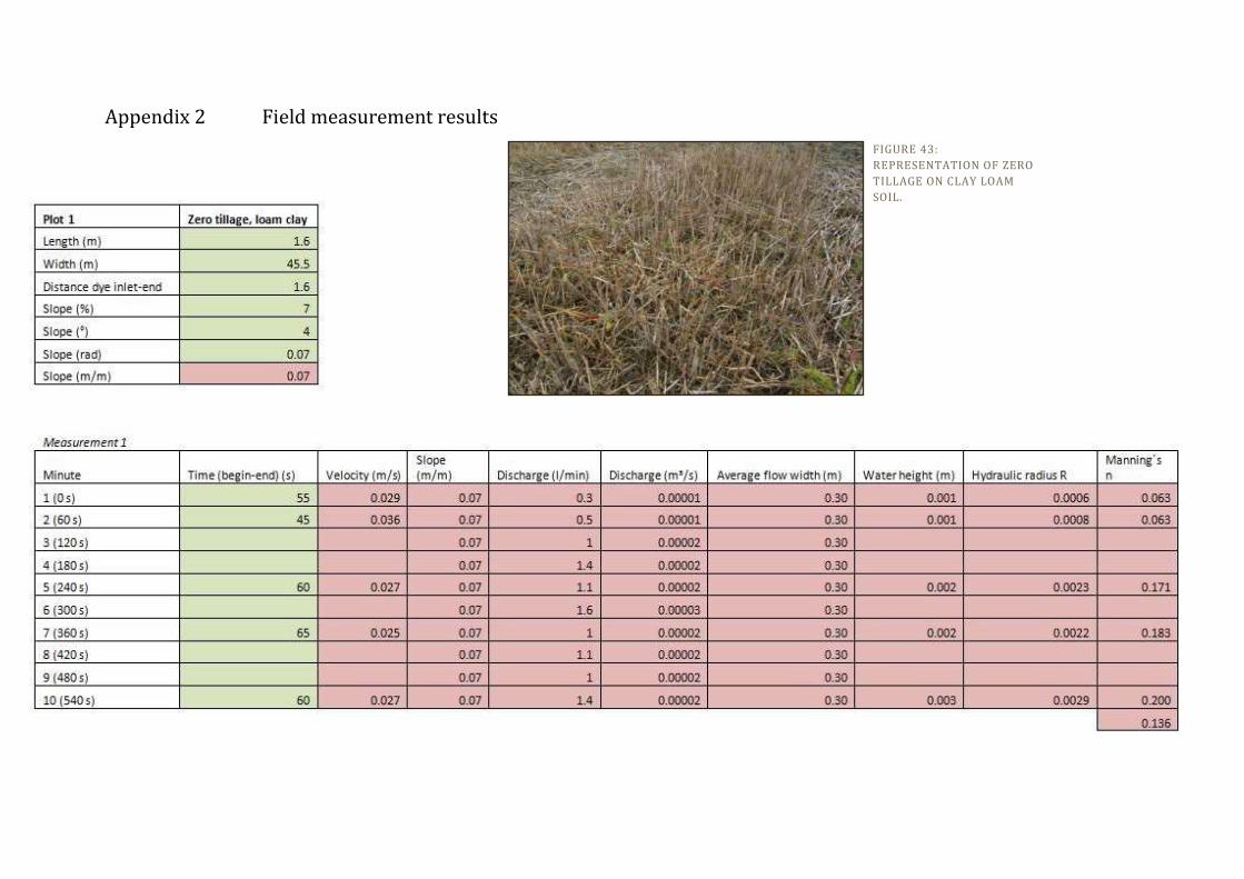
Appendix 2 Field measurement results

FIGURE 43:

REPRESENTATION OF ZERO

TILLAGE ON CLAY LOAM

SOIL.

33

34

FIGURE 44:

REPRESENTATION OF

TILLED CLAY LOAM SOIL.

35

36

37

FIGURE 45:

REPRESEENTATION OF

GRASSED SURFACE.

38

39

FIGURE 46:

REPRESENTATION OF

TILLED SANDY SILT SOIL.

40

41

42

FIGURE 47:

REPRESENTATION OF ZERO

TILLEAGE ON SANDY SILT

SOIL.

43

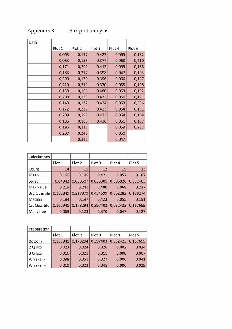
Appendix 3 Box plot analysis

Data

Plot 1 Plot 2 Plot 3 Plot 4 Plot 5

0,063 0,197 0,427 0,065 0,182

0,063 0,155 0,377 0,068 0,210

0,171 0,202 0,412 0,055 0,188

0,183 0,217 0,398 0,047 0,193

0,200 0,170 0,396 0,066 0,147

0,219 0,219 0,370 0,055 0,198

0,158 0,166 0,480 0,053 0,152

0,200 0,123 0,472 0,066 0,127

0,148 0,177 0,434 0,053 0,236

0,172 0,227 0,423 0,054 0,191

0,209 0,197 0,423 0,058 0,168

0,185 0,180 0,436 0,051 0,197

0,196 0,217 0,059 0,237

0,207 0,241 0,050

0,241 0,047

Calculations

Plot 1 Plot 2 Plot 3 Plot 4 Plot 5

Count 14 15 12 15 13

Mean 0,169 0,195 0,421 0,057 0,187

Stdev 0,04942 0,033507 0,033305 0,006926 0,032403

Max value 0,219 0,241 0,480 0,068 0,237

3rd Quartile 0,199849 0,217979 0,434699 0,062282 0,198274

Median 0,184 0,197 0,423 0,055 0,191

1st Quartile 0,160941 0,173294 0,397403 0,052423 0,167655

Min value 0,063 0,123 0,370 0,047 0,127

Preparation

Plot 1 Plot 2 Plot 3 Plot 4 Plot 5

Bottom 0,160941 0,173294 0,397403 0,052423 0,167655

2 Q box 0,023 0,024 0,026 0,002 0,024

3 Q box 0,016 0,021 0,011 0,008 0,007

Whisker - 0,098 0,051 0,027 0,006 0,041

Whisker + 0,019 0,023 0,045 0,006 0,039

45

FIGURE 48: BOXPLOT OF MANNING'S N VALUES SHOWING THE DEVIATIONS FOR EACH LAND UNIT

0

0.1

0.2

0.3

0.4

0.5

0.6

Plot 1 Plot 2 Plot 3 Plot 4 Plot 5

Box plot Manning's n

Appendix 4 T-test analysis

t-Test: Two-Sample Assuming Unequal Variances 1 loamy clay, zero tillage 2 loamy clay, tilled soil

Variable 1 Variable 2

Mean 0.169386909 0.195191914

Variance 0.00244229 0.001122713

Observations 14 15

Hypothesized Mean Difference 0

df 23

t Stat -1.634352103

P(T<=t) one-tail 0.057899879

t Critical one-tail 1.713871528

P(T<=t) two-tail 0.115799759

t Critical two-tail 2.06865761

t-stat<-T Critical False

t-stat> T Critical False

Null-hypothesis rejected, no convincing differences: plots do not differ significantly

t-Test: Two-Sample Assuming Unequal Variances 4 Sandy silt, tilled soil 5 Sandy silt, zero tillage

Variable 1 Variable 2

Mean 0.05655464 0.186566009

Variance 4.79699E-05 0.001049975

Observations 15 13

Hypothesized Mean Difference 0

df 13

t Stat -14.18833667

P(T<=t) one-tail 1.36836E-09

t Critical one-tail 1.770933396

P(T<=t) two-tail 2.73672E-09

t Critical two-tail 2.160368656

t-stat<-T Critical True

t-stat> T Critical False

Null-hypothesis approved, convincing differences: plots do differ significantly

47

t-Test: Two-Sample Assuming Unequal Variances 2 loamy clay, tilled soil 4 Sandy silt, tilled soil

Variable 1 Variable 2

Mean 0.195191914 0.05655464

Variance 0.001122713 4.79699E-05

Observations 15 15

Hypothesized Mean Difference 0

df 15

t Stat 15.6930039

P(T<=t) one-tail 5.12194E-11

t Critical one-tail 1.753050356

P(T<=t) two-tail 1.02439E-10

t Critical two-tail 2.131449546

t-stat<-T Critical False

t-stat> T Critical True

Null-hypothesis approved, convincing differences: plots do differ significantly

t-Test: Two-Sample Assuming Unequal Variances 1 loamy clay, zero tillage 5 Sandy silt,zero tillage

Variable 1 Variable 2

Mean 0.169386909 0.186566009

Variance 0.00244229 0.001049975

Observations 14 13

Hypothesized Mean Difference 0

df 23

t Stat -1.075340504

P(T<=t) one-tail 0.146686977

t Critical one-tail 1.713871528

P(T<=t) two-tail 0.293373953

t Critical two-tail 2.06865761

t-stat<-T Critical False

t-stat> T Critical False

Null-hypothesis rejected, no convincing differences: plots do not differ significantly

48

t-Test: Two-Sample Assuming Unequal Variances 2 loamy clay, tilled soil 3 Grass

Variable 1 Variable 2

Mean 0.195191914 0.4207355

Variance 0.001122713 0.001109244

Observations 15 12

Hypothesized Mean Difference 0

df 24

t Stat -17.43823785

P(T<=t) one-tail 1.95908E-15

t Critical one-tail 1.71088208

P(T<=t) two-tail 3.91817E-15

t Critical two-tail 2.063898562

t-stat<-T Critical True

t-stat> T Critical False

Null-hypothesis approved, convincing differences: plots do differ significantly