soil physical and hydraulic properties of the upper indus
TRANSCRIPT

Soil Physical and Hydraulic Properties
of the Upper Indus Plain of Pakistan
A Research Report
Manzoor Ahmad Malik
Muhammad Ashraf
Ali Bahzad
Arslan Muhammad Aslam
Pakistan Council of Research in Water Resources Islamabad-Pakistan
2019

Citation:
Malik, M.A., M. Ashraf, A. Bahzad, A. M. Aslam (2019). Soil Physical and Hydraulic
Properties of the Upper Indus Plain of Pakistan. Pakistan Council of Research in Water
Resources (PCRWR), pp. 70.
ISBN 978-969-8469-69-6
© All rights reserved. The authors encourage fair use of this material for non-commercial
purpose with proper citation.
Disclaimer:
The views expressed are those of the authors, and not necessarily those of PCRWR.
Where trade names are used, it does not imply endorsement of, or discrimination
against, any product.

Soil Physical and Hydraulic Properties of the Upper Indus Plain of Pakistan
Manzoor Ahmad Malik
Muhammad Ashraf
Ali Bahzad
Arslan Muhammad Aslam
Pakistan Council of Research in Water Resources Islamabad - Pakistan
2019


i
Acknowledgments
This report is an outcome of the study “Characterizing Hydrology of the Eastern Rivers
of the Indus Plain” under the umbrella project “Strategic Strengthening of Flood
Warning and Management Capacity of Pakistan”. This important study was conducted
with the financial and technical support provided by Japan International Cooperation
Agency (JICA) and United Nations Educational, Scientific and Cultural Organization
(UNESCO). The authors would like to thank Professor Dr. Shahbaz Khan, Director,
Regional Science Bureau for Asia and the Pacific, Jakarta, Indonesia, Ms. Vibeke Jensen,
Country Director, UNESCO Pakistan, Dr. Ai Sugiura, Science Programme Specialist, Policy
Capacity Building, UNESCO House, Jakarta, Indonesia and Mr. Raza Shah Programme
Officer UNESCO, Pakistan for their continuous support to PCRWR.
The authors would also like to thank their colleagues Engr. Faizan ul Hasan Director,
Engr. Ibtisam Asmat, Assistant Director, Engr. Muhammad Abbas, Engr. Muhammad
Aleem, Engr. Sajid Hussain, Mr. Faizan Sabir; Research Associates for assistance and
contribution in data collection, field sampling, laboratory analysis and results
compilation. The authors are also thankful to Mr. Zeeshan Munawar, Assistant for
formatting the report.

ii

iii
FOREWORD
Soil physical and hydraulic properties are of paramount importance for the design
of irrigation and drainage projects, pollutant and solute transport, determining the
soil-water-plant and rainfall-runoff relationships. However, these important
parameters have not been determined in Pakistan. Mostly book values
determined somewhere else have been used for various purposes.
The UNESCO Jakarta Office launched a program in Pakistan entitled “Strategic
Strengthening of Flood Warning and Management Capacity of Pakistan” with the
financial assistance of Japan International Cooperation Agency (JICA). The soil
physical and hydraulic properties are important inputs for flood forecasting
models. Therefore, UNESCO entrusted PCRWR for this task.
A team of PCRWR professionals determined these properties in the Pothwar and
the four Doabs (doab is the area between the two rivers) from the Upper Indus
Plain. These properties include: soil texture, soil organic matter, soil chemical
properties, infiltration rate, moisture-retention curves at the surface, 0.5 m and
1.0 m depths, at the specific grid intervals. For the purpose, PCRWR also
established a state-of-the-art Soil Physics Laboratory.
Determining of these properties from Pothwar (about 2.2 Mha) and four Doabs
(about 11 Mha) and management of data was a huge task. The dedicated efforts
of PCRWR team under the leadership of Dr. Manzoor Ahmad Malik made it
possible and now the report is in your hand.
The data generated and presented are unique and are only possible with the technical and financial support of UNESCO and the JICA. I hope the report will help the researchers and managers to better plan for the development and management of the country’s water resources.
Dr. Muhammad Ashraf Chairman, PCRWR

iv

v
Table of Contents
1. Introduction .......................................................................................................................... 1
2. Theory and Literature............................................................................................................ 2
Theory of Infiltration ..................................................................................................... 2
Soil Moisture Retention and Hydraulic Conductivity .................................................... 5
Effective Hydraulic Conductivity ................................................................................... 6
Lithology of Soil Strata .................................................................................................. 8
3. Pedo-transfer Functions ........................................................................................................ 9
4. Description of the Study Area ............................................................................................. 10
4.1 Pothwar Plateau .......................................................................................................... 10
4.2 Doabs ........................................................................................................................... 10
4.2.1 Doab .................................................................................................................... 10
4.2.2 Thal Doab ............................................................................................................ 10
4.2.3 Chaj Doab ............................................................................................................ 11
4.2.4 Rachna Doab ....................................................................................................... 11
4.2.5 Bari Doab ............................................................................................................. 11
5. Methodology ....................................................................................................................... 13
5.1 Infiltration Rate Measurement ................................................................................... 13
5.2 Collection of Soil Samples ........................................................................................... 17
5.3 Measurement of Soil Moisture Retention at Low Suction .......................................... 19
5.4 Determining Moisture Retention at High Suction ....................................................... 21
5.5 Fitting of Moisture-Retention Function ...................................................................... 22
5.6 Texture Analysis of the Soil Samples ........................................................................... 23
5.7 Determining Soil Organic Matter ................................................................................ 26
5.8 Field Procedure for Electrical Resistivity Survey ......................................................... 26
5.9 Measurement of Soil Chemical Parameters ................................................................ 27
6. Results and Discussion ........................................................................................................ 28
Infiltration Rate ........................................................................................................... 28
Soil Moisture Retention .............................................................................................. 36
Soil Texture Analysis .................................................................................................... 38
Regional Lithological Features .................................................................................... 43
Soil Organic Matter in Pothwar ................................................................................... 47
Chemical Properties of Pothwar Soils ......................................................................... 49
7. Conclusions ......................................................................................................................... 56

vi
References ....................................................................................................................... 57
Annexure - A (Pothwar and Doabs Dataset) ................................................................... 61

vii
List of Figures
Figure 1. A schematic diagram of the conductivity of layered soil profile .......................... 8
Figure 2. Setting of potential and current electrodes for resistivity survey ........................ 9
Figure 3. Geographical map of the survey sites in Pothwar .............................................. 12
Figure 4. Geographical map of the survey sites in Doabs ................................................. 13
Figure 5. Schematic diagram and specifications of Infiltrometer ...................................... 14
Figure 6. Cross bar for hammering the infiltrometer rings into the soil ............................ 15
Figure 7. An angle iron steel bar with steel hooks and spirit level for leveling infiltration
rings and maintaining water depth ...................................................................... 15
Figure 8. Operational set up of Infiltrometer installed in the field ...................................... 17
Figure 9. Steel cans for collection of undisturbed soil samples ........................................ 18
Figure 10. Soil samples stored in duly coded three rack boxes for transporting from the
field ........................................................................................................................... 18
Figure 11. Soil samples stored in the laboratory packed in duly coded surface, middle
and bottom racks of specially managed boxes ................................................. 19
Figure 12. Hein’s Tension Table Assemblies: wall mounting arrangement with
provision of adjusting suction head ..................................................................... 20
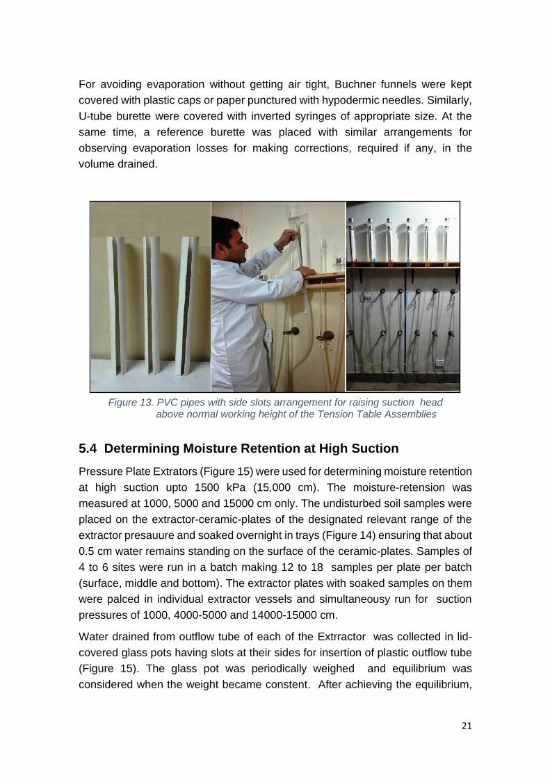
Figure 13. PVC pipes with side slots arrangement for raising suction head above
normal working height of the Tension Table Assemblies ................................ 21
Figure 14. Soaking of soil samples on ceramic pressure plates ....................................... 22
Figure 15. Pressure Plate Extractors set up with drainage from outflow tubes being
collected in glass pots ........................................................................................... 23
Figure 16. Splash proof and controlled length plunger compatible with the standard
cylinder for stirring the soil suspension ............................................................... 24
Figure 17. Texture analysis of surface, middle and bottom soil layers of a pit ............... 25
Figure 18. Soil class identification with standard soil texture classification triangle ...... 25
Figure 19. Infiltration rate of different soil types in Pothwar Region ................................. 30
Figure 20. Horton’s steady-state infiltration rate in Pothwar (surface layer) ................... 31
Figure 21. Horton’s steady-state infiltration rate in Pothwar (middle layer) ..................... 31
Figure 22. Horton’s steady-state infiltration rate in Pothwar (bottom layer) .................... 32
Figure 23. Infiltration rates of different soil types in the Doabs ......................................... 33
Figure 24. Horton’s steady-state infiltration rates in surface layer of Doabs ................... 34
Figure 25. Horton’s steady-state infiltration rates in middle layer of Doabs .................... 34

viii
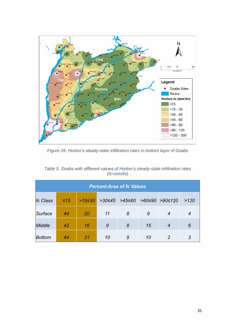
Figure 26. Horton’s steady-state infiltration rates in bottom layer of Doabs .................... 35
Figure 27. Soil moisture retention curves for Pothwar ........................................................ 37
Figure 28. Soil moisture retention curves for Doabs ........................................................... 37
Figure 29. Distribution of soil classes with depth in Pothwar ............................................. 38
Figure 30. Soil types at the surface layer in Pothwar ......................................................... 39
Figure 31. Soil types at the middle layer in Pothwar ........................................................... 39
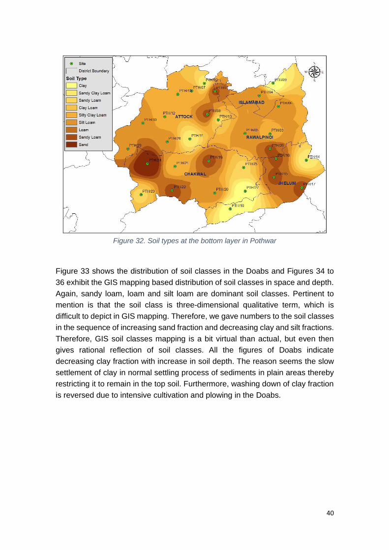
Figure 32. Soil types at the bottom layer in Pothwar .......................................................... 40
Figure 33. Frequency distribution of soil classes with depth in Doabs ............................ 41
Figure 34. Soil types at the surface layer in Doabs ............................................................ 41
Figure 35. Soil types at the middle layer in Doabs .............................................................. 42
Figure 36. Soil types at the bottom layer in Doabs ............................................................. 42
Figure 37. Lithological features at 5 m depth in Pothwar ........................................................ 43
Figure 38. Lithological features at 15 m depth in Pothwar ...................................................... 44
Figure 39. Lithological features at 30 m depth in Pothwar ..................................................... 44
Figure 40. Lithological features at 45 m depth in Pothwar ...................................................... 45
Figure 41. Lithological features at 3 m depth in Doabs ......................................................... 45
Figure 42. Lithological features at 10 m depth in Doabs ....................................................... 46
Figure 43. Lithological features at 50 m depth in Doabs ....................................................... 46
Figure 44. Spatial distribution of soil organic matter in surface layer of Pothwar ........... 48
Figure 45. Spatial distribution of soil organic matter in middle layer of Pothwar ............ 48
Figure 46. Spatial distribution of soil organic matter in bottom layer of Pothwar............ 49
Figure 47. The EC in the surface layer ................................................................................. 50
Figure 48. The EC in the middle (0.5 m depth) layer .......................................................... 51
Figure 49. The EC in the bottom (1.0 m depth) layer ......................................................... 51
Figure 50. SAR in surface layer ............................................................................................. 53
Figure 51. SAR in the middle (0.5 m depth) layer ............................................................... 53
Figure 52. SAR in the bottom (1.0 m depth) layer ............................................................... 54
Figure 53. pH in surface layer ................................................................................................ 54
Figure 54. pH in the middle (0.5 m depth) layer of Pothwar .............................................. 55
Figure 55. pH in the bottom (1.0 m depth) layer .................................................................. 55

ix
List of Tables
Table 1. Coverage per site and No. of sites in each district in Pothwar .......................... 11
Table 2. Coverage per site and No. of sites in each Doab ................................................ 12
Table 3. Correlation between electrical resistivity and hydrogeological conditions ....... 27
Table 4. Pothwar region having different values ofHorton’s steady-state infiltration rate
(fc = mm/hr) ............................................................................................................. 32
Table 5. Doabs with different values of Horton’s steady-state infiltration rates
(fc=mm/hr) ............................................................................................................... 35
Table 6. Pothwar region having different values of organic matter (%) ........................... 47

x

xi
Executive Summary
Soil-water interaction is the key component of hydrological cycle. This interaction is
determined by soil hydraulic properties which in turn depend on soil physical and
chemical properties. Soil physical and chemical properties include texture, bulk density,
organic matter, sodium absorption ratio, EC, pH, etc. Soil hydraulic properties include
infiltration rate and soil moisture-retention characteristics from which saturated-
unsaturated hydraulic conductivity profile can be developed.
The soil physical properties facilitate empirical determination of soil hydraulic properties
using pedotransfer functions. Therefore, these properties have gained prime
importance with rampant growth of computer models such as rainfall runoff, solute
transport, groundwater recharge, crop growth, nutrient uptake, irrigation scheduling
etc. Use of such models is important for rapid research outcome, scenario development,
forecasting hydrological events and impact assessment of best management practices.
All these models require soil physical and hydraulic properties as fundamental input in
one form or the other. However, in spite of their great importance, these properties
have not been determined in Pakistan. Most of times, these values have been taken
from the literature, that have been determined elsewhere.
PCRWR carried out this study for the Upper Indus Plain for determining basin’s soil
physical, hydraulic and chemical properties together with soil lithology at 30 points in
the Pothwar Region and 96 in Doabs (the area between two rivers). The methodology
adopted was hydrometer method for soil texture, improved double-ring infiltrometer
for infiltration rate, tension table assembly and pressure-plate extractor for soil
moisture-retention characteristics, burning weight loss method for organic matter, oven
dried weight for bulk density, saturated paste extract for chemical properties and
resistivity survey with terrameter for soil lithology.
The results indicate that sandy loam, loam and silt loam are dominant soils in Pothwar
and Doabs. However spatially, sandy loam decreases with depth in the Pothwar region,
whereas clay contents decrease with depth in the Doab’s. Moisture-retention
characteristics are more variable for similar classes of soils in the Pothwar than in Doabs.
The soil with infiltration rates up to 45 mm/hr are dominant in the Pothwar, whereas
the rates up to 30 mm/hr are dominant in Doabs. Lithological strata are more diverse in
Pothwar Region as compared to Doabs where it is almost uniform. Soil organic matter
contents in the Pothwar vary from 0.2 to 2.5%. No hazards of sodicity and/or salinity are
noticed in the Pothwar region.

xii

1
1. Introduction
The Indus Basin has experienced the history of devastating floods of which the
most recent were unprecedented. These floods were mainly because of climate
change based rainstorms combined with glacier lake outburst, glacier surge or
glacier advancement rejuvenation. The flood 2010 was first of its kind in the
region and was most disastrous in the history of the Indus Basin. A record-
breaking rainfall of 274 mm occurred in Chitral in just 24 hours. The floods
affected 20 million people, with 200 casualties apart from damaging
infrastructure, livestock, crops and millions of houses (Kirsch et al., 2012).
Frequency of such events is likely to increase in the near future owing to climate
change implications. However, capacity of Pakistan for preparedness,
management and flood early warning is limited. Hydrological models are state of
the art technology for flood forecasting and early warning. These models require
rainfall data, topographical features, land use and land cover data, and hydraulic
parameters of the soil profile. Satellite imagery and remote sensing has made it
easy to acquire rainfall and its distribution data, topographical features, land cover
and land use data. However, information on soil physical and hydraulic
properties, which are pre-requisites for hydrological models for partitioning rainfall
into infiltration and runoff components, are almost non-existence.
Pedo-transfer functions developed elsewhere in the world are used to fill this data
gap. For distributed modeling, fine scale estimation of soil physical and hydraulic
properties are of prime importance. The pedo-transfer functions are region and
area specific. Pakistan has so far neither developed pedo-transfer functions nor
hydraulic characteristics of its soils. Use of pedo-transfer functions developed
elsewhere also lead to inaccurate results in the distributed hydrological modeling
carried out for specific regions such as the Indus Basin (Lin et al., 2005).
Moreover, rapid population growth, urbanization, and industrialization have led
groundwater mining in many parts of the country. It has been estimated that water
table is rapidly falling in more than half of the 45 canal commands of the basin.
The falling trend of water table is more pronounced in urban settlements. For
regulating and managing groundwater development, knowledge of safe yield is
very important.
Safe yield is best estimated if accurate data of infiltration and surface-
groundwater interaction are available. The soil hydraulic properties are of vital
importance for surface-groundwater interaction and determination of seepage
rate. Soil physical and hydraulic properties are further affected by its chemical
properties. Data on all these aspects are prerequisite for modeling flow regimes,

2
flood forecasting and solute transport. Therefore, the focus of this report is to
determine soil physical, chemical and hydraulic properties in Pothwar and in the
four Doabs.
2. Theory and Literature
Theory of Infiltration
Infiltration is the vertical entry of water into the soil surface, whereas the entry of
water per unit time is called infiltration rate. It is the most crucial component of
hydrologic cycle for sustaining life on the earth through its diversified physical,
biological and chemical processes. It is important, inter alia, for flood forecasting,
irrigation management, erosion control, pollutant transport etc. Therefore,
scientists are endeavoring to model it since the start of twentieth century and now
various models are available. These models are categorized into physical, semi-
physical and empirical. Richard (1931) model is physical based derived from
Darcy’s law. The model involves complex computations and requires soil physical
parameters in terms of conductivity and soil suction head, the measurement of
which is time and cost intensive. Advancement in computer technology has
though reduced computation difficulties but physical data such as unsaturated
hydraulic conductivity are still the major limitations for its usage (Turner, 2006).
The first semi empirical model is of Green and Ampt (1911) which was also
derived from Darcy’s equation but with simplifying assumptions and is given by
Equation 1.
( ) ( )02 1
2 1 0 f
f f f fs s s s
f
z Hdh h h z Hi K K K K
dz z z z z
− = − = − = −
+ − +− + −=
− − ……….….(1)
Where:
H = the depth of ponding (mm),
Ks = saturated hydraulic conductivity (mm/hr),
i = flux at the surface (mm/h) and is negative,
= suction at wetting front (negative pressure head) and
= distance to suction front (mm).
The assumptions of the Green and Ampt model are that the wetting front is well
defined and advances at the same rate through the entire depth; and moisture
contents over and above the wetting front remain constant. The assumptions, in
fact, do not exist in the real field conditions. Despite unrealistic real field
assumptions, Green and Ampt model worked well over variety of field and

3
lithological conditions (Childs and Bybordi, 1969; Hillel and Gardner, 1970;
Turner, 2006).
Phillip (1957) model is also physical based as it is shortened form of infinite series
solution of Richard (1931) partial differential equation. The infiltration and
cumulative infiltration forms of the Philip’s model are given by Equations 2 and 3.
1
2( )I t St At= + ………………………………………..……………………….(2)
1
21
( )2
i t St A−
= + ………………………………………………………………..(3)
Where I(t) is cumulative infiltration (mm) as function of time; i(t) is infiltration rate
at given time (mm/hr); t is time (hr); S is sorptivity (mm/hr1/2); A is constant
parameter.
The parameter “A” of the Philip’s equation is empirically correlated with saturated
conductivity by Ksat = A/n. The value of n varies between 0.3 to 0.7 depending
on initial moisture content and time of infiltration (Philip, 1969) and even may
ultimately approach to 1.0 after a long time (Hillel, 1982) when the infiltration rate
curve becomes parallel to horizontal axis. However, inherently Philip’s equation
does not yield steady-state condition. As such, there is no consensus on a single
value of the parameter “n” and often hypothetically a value of n = 0.667 is used
for determining saturated hydraulic conductivity (Batkova, 2013). Philip’s model
can be considered as modified form of Kostiakov (1932) model given by
Equation 4.
p kf K t −= …………………………………..……………..……………….. (4)
Where:
pf = infiltration rate (mm/hr);
t = time since start of infiltration (hr);
kK = (mm) and ⍺ (unit-less) are empirical constants to be determined from
infiltration data.
If the value of ⍺ is taken as 0.5, the Kostiakov equation becomes equivalent to
Philip’s equation.
Although Kostiakov model is simple and widely used, but the main reservation is
that it takes initial infiltration as infinite, which exponentially decreases without
4
achieving any steady-state condition, that is against the real field conditions
(Haverkamp et al., 1987; Naeth, 1988). This deficiency is covered in Horton
(1940) model, which duly incorporates steady-state infiltration rate. The
cumulative and infiltration rate forms of Horton model are given by Equations 5
and 6, respectively.
( ) 1o c pp c p
f f ktF t f t e
k
−
+ −
−= ……………………………..……………….…..(5)
( ) pkt
p c o cf f f f e−
= + − ……………………………………….………………(6)
Where, F is cumulative infiltration (mm); fp is infiltration rate (mm/hr) at given time;
fo is initial infiltration rate (mm/hr); fc is steady-state infiltration rate (mm/hr); k is
the decay constant specific to the soil. Each of the infiltration models has its own
limitations and facilitations. Green and Ampt equation despite having over
simplified assumptions is still the most widely used amongst the physical based
models. However, Horton empirical model better accounts for the soil and field
conditions for which infiltration estimates are to be made as it derives parameters
from the measured data of the same soil under field conditions. Therefore,
according to Bevin (2004), Horton’s empirical model incorporates hydrological
and surface conditions of infiltration process in a more complete way than is
presented in literature. Turner (2006) has presented comprehensive review of the
theory of infiltration.
Telis (2001) carried out double ring infiltration measurements at 23 sites in
Calosahatchee River Basin for estimating infiltration rates of saturated soils. His
data were highly scattered despite use of Marriott flask arrangement. He
regressed the measured data on Horton model after removing outliers from five
sites. His measured data on seven sites could not be regressed on Horton model
due to early steady-state infiltration. He estimated infiltration rates of the sites by
averaging data after 20 minutes’ test when the infiltration rate became constant.
The determined infiltration rates were 98 to 1150 mm/hr in flatwoods; 34 to 66
mm/hr in rocks or clay layer; and 25 to 55 mm/hr in open grass land. His final
infiltration rates occurred at about 20-30 minutes. He acknowledged that the
scatter data was due to difficulties in precise measurement of water infiltrated
over incremental time intervals. He reported that the process of infiltration is

5
complex due to interaction of soil texture, soil structure, and antecedent moisture
content and soil surface conditions.
Richard and Gifford (1981) regressed the data of 2090 rangeland sites on Phillip’s
model and reported that only 72% sites had R2 greater than 0.75. He further
reported that extremely low values of R2 resulted from non-variability of infiltration
rate resulting from high antecedent moisture contents and hence nearly zero
value of sorptivity (S). They further reported that low value of R2 on many other
sites was due to unexplainable behavior of data and insufficient flexibility of the
model. They elaborated that the model fitted differently for different data and
opined that R2 simply gave an index but not complete picture of data fit. According
to them, sorptivity (S) decreases fivefold in the first five minutes. Abdulkadir et al.
(2011) showed that Horton Model fitted better on his data of 15 sites with mean
R2 value of 0.811 for loam soils in arid and semi-arid regions of Nigeria. Their
steady state infiltration rates varied between 6-48 mm/hr.
An important feature of Horton’s equation is that the steady state infiltration rate
is its built-in parameter. The steady state infiltration rate is considered as the
index of field saturated hydraulic conductivity (Ksat). Phillip (1969) stated that Ksat
might be semi-empirically related with constant “A” of his equation of infiltration.
According to his relationship, field saturated hydraulic conductivity (Ksat) is some
multiple of “A” where value of the multiple varies between 0.3 and 0.7 depending
on initial moisture content. According to Hillel (1982), the multiple may be 1.0 as
the filed saturated hydraulic conductivity practically ultimately approaches steady
state infiltration.
The literature reveals that various infiltration models are available but their usage
depends on how best they fitted the measured data and intended determination
of requisite parameters. If the purpose is to determine steady state infiltration rate,
or field saturated conductivity, then Horton’s model has edge that it directly gives
consistent value of the same due to being its built-in parameter.
Soil Moisture Retention and Hydraulic Conductivity
The correlation of steady state infiltration with field saturated hydraulic
conductivity is important as the latter is required for developing saturated-
unsaturated conductivity profile of soils using van Genuchten (1980) closed form
conductivity function given by Equation 7.

6
( )( ) ( )
( )
21
2
1 1
1
mn n
s mn
K K
−− − +
= +
………………….………… (7)
Where
( )K = hydraulic conductivity at given suction head (cm);
sK = saturated hydraulic conductivity (cm/s); and
ψ = suction head (cm).
𝑚 = 1 − 1 𝑛⁄ ; and α and n are parameters derived from van Genuchten (1980)
soil moisture retention function where value of n>0. However, if the value of n>2,
the form of unsaturated conductivity function becomes as given by Equation 8
while maintaining consistency of the parameter’s definition given above.
( )( ) ( )
( )
2
2
1 1
1
mn n
s mn
K K
−− − +
= +
……………..…………...….. (8)
The other parameters of the Equations 7 and 8 are derived from van Genuchten
(1980) soil moisture retention function given by Equation 9.
( )( )
11
1n
s rr
n
−
−= +
+
………………..………………………… (9)
Where
( ) = the water retention (cm3/cm3) at given soil suction;
𝜓 = suction pressure (cm of water);
s = saturated water content (cm3/cm3);
r = residual water content (cm3/cm3);
𝛼 = inverse of the air entry suction, (cm−1); and
n = slope of the curve reflecting pore size distribution (dimensionless).
Effective Hydraulic Conductivity
As mentioned before, the field saturated hydraulic conductivity (Ksat) is
considered equivalent to steady-state infiltration rate as suggested by Hillel
(1982). The so determined saturated-unsaturated conductivity profile provides
input requirements of physical based hydrological models involving saturated-
unsaturated flow within the soil profile. However, soils or earth profile are

7
heterogeneous in nature and it is more efficient to determine effective conductivity
of soil strata than incorporating individual heterogeneities. Therefore, effective
hydraulic conductivity is often used for taking advantage of that efficiency
(Gohardoust et al., 2017). The effective conductivity of layered profile depends
on orientation of soil layers or lithology (Gohardoust et al., 2017). Under saturated
conditions, effective conductivity is harmonic mean of conductivity of individual
layers if the layers are perpendicular to flux and simple arithmetic mean if the
layers are parallel to the flux (Zhu, 2008). The equation for determining effective
vertical conductivity by harmonic mean of horizontal layered soil profile as shown
in Figure 1 is given by Equation 10.
131 2
1 2 3
.....
nT T
e
in i
n i
d dK
d d dd d
K K K K K
=
= =
+ +
……………………….….…….. (10)
Where:
1d , 2d , 3d …. nd are depths of the individual soil layers and 1K , 2K , 3K , ……
nK are their corresponding conductivities up to nth layer;
Td is the total depth of the layered soil profile; and
eK is the effective conductivity of the soil profile.
Equation 10 works well for saturated conditions (Warrick, 2005). However, its
application for unsaturated conditions becomes difficult due to non-linear relation
between conductivity and degree of saturation (Zhu, 2008). Zhu and Warrick
(2012) found that harmonic mean based hydraulic conductivity works better for
infiltration than evaporation. Gohardoust et al. (2017) demonstrated that effective
unsaturated hydraulic conductivity falls between geometric and harmonic means
of the conductivities of the individual layers. Whatever the case may be, an
estimation of the stratification or lithology of soil strata is required for determining
effective conductivity for the entire range of saturated and unsaturated conditions.
To meet that requirement, lithology of vadose zone can be determined physically.
For deeper layers, well logs are prepared through drilling which is time, labor and
cost intensive. However, resistivity survey provides the most economical tool for
mapping lithological features of the soil.

8
Figure 1. A schematic diagram of the conductivity of layered soil profile
Lithology of Soil Strata
As discussed above, lithology of soil strata and depth and nature of material in
each layer is important to determine effective saturated-unsaturated hydraulic
conductivity of the strata for adding efficiency and simplicity to simulation.
Electrical Resistivity is the state-of-the-art technology to determine lithological
features of soil strata and quality of water stored therein.
Different techniques are used for lithological study and water quality assessment.
Our requirement in this study was lithological features only. For that purpose,
Schlumberger electrode configurations is mostly used. In this method, four
electrodes are placed along a straight line on the earth surface in the order of AM
NB with AB 5 MN. The general setting of the potential and current electrodes
and distribution of current as well as potential lines is given in Figure 2.
Terrameter is used for the field data collection. This instrument works on the basis
of Ohm's laws. The governing equation is written as:
K VR
I
− ……………………………………………………….…………. (11)
Where:
R = Resistivity (Ohm-meter);
V = Voltage or potential drop (milli-Volt)
Layered media Equivalent
homogeneous
h14
K1
K2
K
d1
d2
d3
h1
h2
h3
h4
q h1
h1
4
h4
dT
q
Ke

9
I = Current (milli-ampere);
K = Constant of proportionality or 2𝜋𝑎; where 𝜋 is 3.14159 and “𝑎” is spacing
between the two electrodes.
Figure 2. Setting of potential and current electrodes for resistivity survey
3. Pedo-transfer Functions
Determining soil moisture-retention and hydraulic characteristics from
comparatively easily measurable soil physical properties are called pedo-transfer
functions (Bouma, 1989). Pedo-transfer functions are regression analysis based
empirical equations, which correlate soil moisture retention and hydraulic
parameters with soil texture, bulk density, organic matter etc. Such functions
available in literature are regions specific. Whereas, indigenously determined soil
physical and hydraulic properties can be used to fulfil input requirements of
physical based models for improving reliability of their outputs.
10
4. Description of the Study Area
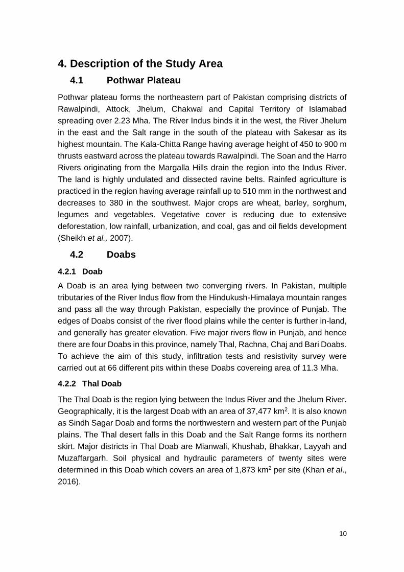
4.1 Pothwar Plateau
Pothwar plateau forms the northeastern part of Pakistan comprising districts of
Rawalpindi, Attock, Jhelum, Chakwal and Capital Territory of Islamabad
spreading over 2.23 Mha. The River Indus binds it in the west, the River Jhelum
in the east and the Salt range in the south of the plateau with Sakesar as its
highest mountain. The Kala-Chitta Range having average height of 450 to 900 m
thrusts eastward across the plateau towards Rawalpindi. The Soan and the Harro
Rivers originating from the Margalla Hills drain the region into the Indus River.
The land is highly undulated and dissected ravine belts. Rainfed agriculture is
practiced in the region having average rainfall up to 510 mm in the northwest and
decreases to 380 in the southwest. Major crops are wheat, barley, sorghum,
legumes and vegetables. Vegetative cover is reducing due to extensive
deforestation, low rainfall, urbanization, and coal, gas and oil fields development
(Sheikh et al., 2007).
4.2 Doabs
4.2.1 Doab
A Doab is an area lying between two converging rivers. In Pakistan, multiple
tributaries of the River Indus flow from the Hindukush-Himalaya mountain ranges
and pass all the way through Pakistan, especially the province of Punjab. The
edges of Doabs consist of the river flood plains while the center is further in-land,
and generally has greater elevation. Five major rivers flow in Punjab, and hence
there are four Doabs in this province, namely Thal, Rachna, Chaj and Bari Doabs.
To achieve the aim of this study, infiltration tests and resistivity survey were
carried out at 66 different pits within these Doabs covereing area of 11.3 Mha.
4.2.2 Thal Doab
The Thal Doab is the region lying between the Indus River and the Jhelum River.
Geographically, it is the largest Doab with an area of 37,477 km2. It is also known
as Sindh Sagar Doab and forms the northwestern and western part of the Punjab
plains. The Thal desert falls in this Doab and the Salt Range forms its northern
skirt. Major districts in Thal Doab are Mianwali, Khushab, Bhakkar, Layyah and
Muzaffargarh. Soil physical and hydraulic parameters of twenty sites were
determined in this Doab which covers an area of 1,873 km2 per site (Khan et al.,
2016).

11
4.2.3 Chaj Doab
The Chaj Doab is the region lying between the Chenab River and the Jhelum
River, with an area of 13,660 km2 and thus area wise it is the smallest Doab. Its
name comes from the first syllables of the names of the two rivers in-between of
which it falls. It forms the central and northeastern part of Punjab plains. Major
districts in this Doab are Gujrat, Mandibahauddin and Sargodha. Ten sites were
covered in Chaj Doab thereby making a grid size of 1,366 km2 per site.
4.2.4 Rachna Doab
The Rachna Doab is between the Ravi and Chenab Rivers and goes all the way
up to the southern end of Kashmir valley. It consists of the main regions of Punjab,
and forms the central and eastern part of it. With its geographical area of
31,331km2, it forms the second largest Doab of the Indus Plain. Major districts in
Rachna Doab are Faisalabad, Gujranwala, Narowal, Sialkot, Nankana Sahib,
Sheikhupura and Toba Tek Singh. Sixteen sites were covered in this Doab,
which provides a grid of 1,958 km2 per site.
4.2.5 Bari Doab
The Bari Doab forms the central and southeastern end of Punjab, and has an
area of 29,649 km2. It is the Doab between the Ravi River, the River Bias and the
Sutlej River. Major districts are Khanewal, Multan, Sahiwal, Okara, Kasur and
Lahore. Twenty sites were covered in this Doab, with a grid of 1,482 km2 per site.
Geographical map of survey sites in Pothwar is given in Figure 3, while districts
covered and coverage per district is shown in Table 1. Similarly, geographical
map of survey sites in Doabs is given in Figure 4, while coverage per Doab is
shown in Table 2.
Table 1. Coverage per site and No. of sites in each district in Pothwar
District Area (grid interval) No. of Sites
Rawalpindi/Islamabad 1015 km2 (32 km x 32 km) 6
Jhelum 698 km2 (26 km x 26 km) 5
Attock 602 km2 (25 km x 25 km) 11
Chakwal 836 km2 (29 km x 29 km) 8
Total 30

12
Figure 3. Geographical map of the survey sites in Pothwar
Table 2. Coverage per site and No. of sites in each Doab
Doab Area (grid interval) No. of Sites
Thal Doab 1674 km2 (41 km x 41 km) 20
Chaj Doab 1366 km2 (37 km x 37 km) 10
Rachna Doab 1958 km2 (44 km x 44 km) 16
Bari Doab 1482 km2 (38 km x 38 km) 20
Total 66

13
Figure 4. Geographical map of the survey sites in Doabs
The distribution of the pits was denser in Pothwar due to more heterogeneity in
geology than in Doabs. Geographical area of Pothwar is 22,254 km2 and the grid
size was 27.5 km × 27.5 km. In Doabs, the sampled grid size was 41.5 km × 41.5
km over the geographical area of 113,085 km2. However, the distribution of grids
was uniform in both the regions.
5. Methodology
5.1 Infiltration Rate Measurement
For carrying out infiltration rate, double-ring Infiltrometers were used (Figure 5).
The upper 15 cm half of each of the ring was reinforced with additional steel plates
of 12 gauge for avoiding damage to the rings while driving into the ground. The
top edges of the rings were further reinforced with U-collars steel strips. For
carrying out the infiltration tests, a step-wise pit was dug having provision for

14
carrying out test at the surface, 0.5 m and 1.0 m depths to accommodate 60 cm
diameter Infiltrometers. The Infiltrometers were set on the surface with cross bar
on the top (Figure 6). The cross bar was then hammered with 2 kg hammer until
half of the ring drove into the soil. The outer ring was driven first and then the
inner one until they attain the same horizontal level. The horizontal level was
checked by placing a 20 cm spirit level on an angle iron placed on top of the rings.
The angle iron bar was provided with three hooks underneath (Figure 7) for
maintaining the same level of water in the outer and the inner rings.
Figure 5. Schematic diagram and specifications of Infiltrometer

15
Figure 6. Cross bar for hammering the infiltrometer rings into the soil
Figure 7. An angle iron steel bar with steel hooks and spirit level
for leveling infiltration rings and maintaining water depth

16
The outer ring was filled first to the required level and the inner ring was then filled
to the same level. The water in both the rings was maintained at the same level
using lower end tips of the hooks of the angle iron bar as a benchmark. The water
feeding mechanism comprised 35-liter containers with taps. For feeding the outer
ring, a plastic hosepipe was fitted to the tap of the water container and placed the
other end in the outer ring. The tap was opened and persistently adjusted to the
extent of maintaining constant head of 10 cm in the ring. For feeding water in the
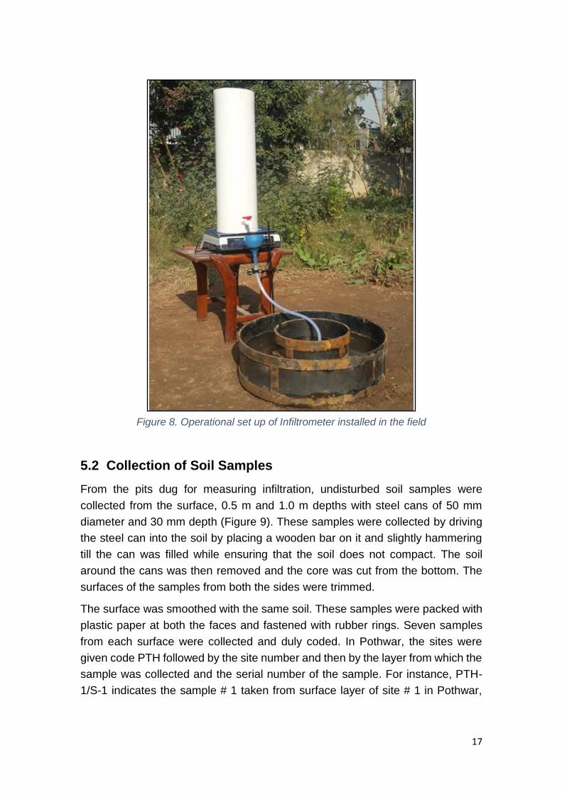
inner ring, water-filled container was placed on a weighing balance (Figure 8).
A funnel-pipe-stand arrangement (Figure 8) was made to pour the water into the
inner-ring. It was ensured that the funnel-pipe-stand arrangement does not touch
the tap of the container placed on the weighing balance. The tap of the container
on the weighing balance was opened and persistently adjusted to the extent of
maintaining the requisite constant head. With this arrangement, the decrease in
weight of the container at intermittent time intervals was recorded.
The total reduction in the weight at any time lapse gave cumulative weight (or
volume) of water infiltrated. That was converted to the cumulative depth infiltrated
by dividing with cross section of the inner-ring. That set up generated good quality
data of cumulative infiltration vs time. The cumulative infiltration data was
recorded for 3-4 hours and fitted against Philip’s (1957) Equations 2-3 and
Horton’s (1940) infiltration functions given by Equations 5 and 6.
The curve fitting by minimizing the least squares difference using solver
command of Microsoft Excel gave the optimized values of parameters “S” and
“A” of the Philip’s equation (Eq. 2). The optimized values of “S” and “A” were then
used to determine infiltration rate (Eq. 3). Similarly, Horton’s form of cumulative
infiltration was used (Eq. 5) as derived from instantaneous infiltration rate (Eq. 6).
The infiltration parameters of Philip’s and Horton’s models were determined by
fitting the models on the recorded data of infiltration tests.
17
Figure 8. Operational set up of Infiltrometer installed in the field
5.2 Collection of Soil Samples
From the pits dug for measuring infiltration, undisturbed soil samples were
collected from the surface, 0.5 m and 1.0 m depths with steel cans of 50 mm
diameter and 30 mm depth (Figure 9). These samples were collected by driving
the steel can into the soil by placing a wooden bar on it and slightly hammering
till the can was filled while ensuring that the soil does not compact. The soil
around the cans was then removed and the core was cut from the bottom. The
surfaces of the samples from both the sides were trimmed.
The surface was smoothed with the same soil. These samples were packed with
plastic paper at both the faces and fastened with rubber rings. Seven samples
from each surface were collected and duly coded. In Pothwar, the sites were
given code PTH followed by the site number and then by the layer from which the
sample was collected and the serial number of the sample. For instance, PTH-
1/S-1 indicates the sample # 1 taken from surface layer of site # 1 in Pothwar,

18
and similarly PTH-1/B-7 is sample # 7 taken from the bottom layer of the same
site.
A three-rack stacked-box arrangement was used for systematic storage and
carriage of the samples (Figure 10). Each rack of the box having capacity for
seven samples was marked from bottom to top as “B” for samples of the bottom
layer (1.0 m depth), “M” for samples of the middle layer (0.5 m depth) and “S” for
samples of the surface layer. The rack-stacked box was also marked for the site
number (Figure 11). The so managed system for placement of the samples
facilitated comfortable storage, carriage and foolproof management and
retrieving the samples from the bulk stock.
Figure 9. Steel cans for collection of undisturbed soil samples
Figure 10. Soil samples stored in duly coded three rack boxes
for transporting from the field

19
Figure 11. Soil samples stored in the laboratory packed in duly coded surface,
middle and bottom racks of specially managed boxes
5.3 Measurement of Soil Moisture Retention at Low Suction
For maintaining consistency in handling samples in the laboratory for moisture-
retention measurements, Sample # 1 of each layer of the site was used at low
suction with Hein’s Tension Table Assembly (Hein’s Apparatus). Hein’s
Assemblies were developed from grade-5 sintered glass Buchner funnels of 70
mm internal diameter. The stem of the funnel was attached through 12 mm
flexible plastic pipe to 50 ml burette for making U-tube arrangement. A set of 30
such assemblies were fixed along wall using a wooden rack arrangement with
necessary provisions for adjusting suction head (Figure 12). Each of the Hein’s
funnel was duly primed ensuring that no air bubble remains in the U-tube
assembly before placing the soil samples in the Hein’s funnel. Before carrying out
moisture retention tests at low suction, the funnels were tested for safe range of
air entry value and no air bubbles were detected until 170 cm suction head. Being
on the safer side, 150 cm was considered as the practical suction limit in the
Hein’s Assembly. Soil samples were placed in the funnel when about 0.5 cm
water depth was available at the surface of the funnel bottom at equilibrium with
water level in the U-Tube.
20
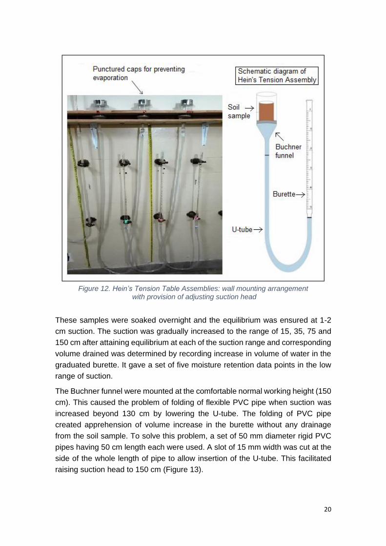
Figure 12. Hein’s Tension Table Assemblies: wall mounting arrangement with provision of adjusting suction head
These samples were soaked overnight and the equilibrium was ensured at 1-2
cm suction. The suction was gradually increased to the range of 15, 35, 75 and
150 cm after attaining equilibrium at each of the suction range and corresponding
volume drained was determined by recording increase in volume of water in the
graduated burette. It gave a set of five moisture retention data points in the low
range of suction.
The Buchner funnel were mounted at the comfortable normal working height (150
cm). This caused the problem of folding of flexible PVC pipe when suction was
increased beyond 130 cm by lowering the U-tube. The folding of PVC pipe
created apprehension of volume increase in the burette without any drainage
from the soil sample. To solve this problem, a set of 50 mm diameter rigid PVC
pipes having 50 cm length each were used. A slot of 15 mm width was cut at the
side of the whole length of pipe to allow insertion of the U-tube. This facilitated
raising suction head to 150 cm (Figure 13).
21
For avoiding evaporation without getting air tight, Buchner funnels were kept
covered with plastic caps or paper punctured with hypodermic needles. Similarly,
U-tube burette were covered with inverted syringes of appropriate size. At the
same time, a reference burette was placed with similar arrangements for
observing evaporation losses for making corrections, required if any, in the
volume drained.
Figure 13. PVC pipes with side slots arrangement for raising suction head
above normal working height of the Tension Table Assemblies
5.4 Determining Moisture Retention at High Suction
Pressure Plate Extrators (Figure 15) were used for determining moisture retention
at high suction upto 1500 kPa (15,000 cm). The moisture-retension was
measured at 1000, 5000 and 15000 cm only. The undisturbed soil samples were
placed on the extractor-ceramic-plates of the designated relevant range of the
extractor presauure and soaked overnight in trays (Figure 14) ensuring that about
0.5 cm water remains standing on the surface of the ceramic-plates. Samples of
4 to 6 sites were run in a batch making 12 to 18 samples per plate per batch
(surface, middle and bottom). The extractor plates with soaked samples on them
were palced in individual extractor vessels and simultaneousy run for suction
pressures of 1000, 4000-5000 and 14000-15000 cm.
Water drained from outflow tube of each of the Extrractor was collected in lid-
covered glass pots having slots at their sides for insertion of plastic outflow tube
(Figure 15). The glass pot was periodically weighed and equilibrium was
considered when the weight became constent. After achieving the equilibrium,

22
the samples were removed, oven dried at 105 oC for more than 24 hours and
determined dry bulk densities and gravimetric moisture contents. Volumetric
moisture contents were determined by multiplying garimetric moisture content
with dry bulk density of the corresponding sample. Average bulk density of each
profile of the site was determined by average of the corresponding samples.
Figure 14. Soaking of soil samples on ceramic pressure plates
5.5 Fitting of Moisture-Retention Function
The moisture-retention data sets were determined with the Tension Table
Assemblies comprisng five data sets and those of Pressure-Plate Extractors
consisting of three data sets. The collated eight data sets were regressed on van
Genuchten moisture-retension function (van Genuchten 1980) given by Equation
9. For regression analysis, sum of the least squared differences between
measured and fitted values was used by optimizing the 𝜃𝑟, 𝛼 and n parameters
of Equation 9 using “Solver” command of Microsoft Excel. The set of constraints
for the parameters optimization in the regression analysis was as below.
=> volumetric moisture content at 1-2 cm suction,
𝜃𝑟 >= 0.00001, 𝛼 >= 0.00001 and n >= 1.
The saturated moisture contents so determined were considered as moisture
retention at zero suction. The observed and fitted data were prepared in graphical

23
form as a fraction of moisture content on Y-axis and suction in centimeters on
logarithmic X-axis.
Figure 15. Pressure Plate Extractors set up with drainage from outflow tubes being collected in glass pots
5.6 Texture Analysis of the Soil Samples
Hydrometer method was used for texture analysis. The oven dried samples
becoming redundant after moisture retention were used for the purpose. The
oven dried sample was crushed with mortar-pestle and passed through 2 mm
sieve. A 50 gm sieved sample was taken in 1000 ml beaker and soaked for 4-8
hours by adding 200 ml distilled water and 50 ml of 10% solution of sodiumn-
hexa-metaphosphate. The soked sample was shaked for 5-10 minutes in
mechanical shaker. The entire contents of the shaker were poured into 1000 ml
standard cylinder and made to the volume of 1000 ml by adding distilled water. A
batch of three or six samples was prepared at a time.
The soil suspension in 1000 ml standard cylinder was shaked with a specially
prepared plunger (Figure 16). Hydrometer readings in the duly shaked soil
suspenions were taken berween 40-45 seconds after shaking for concentration
of silt and clay. Similarly 2 hours readings were also taken for concentration of
clay only (Figure 17). After each of the reading, temprature of the soil suspension

24
was recorded. The zero error of hydrometer was also detrermined by taking
reading in distilled water at the same temprature. Before that, blank solution was
prepared by adding 50 ml of 10% solution of sodium-hexa-metaphosphate in
distilled water to make the volume to 980 ml. The 20 ml reduced volume of the
blank solution was for provision of volume of 50 gm of soil paricles assumung
particle density of 2.5 g/ml.
All the readings in the soil suspension were corrected for the zero error.
Moreover, temprature difference error due to temprature over or below the
standard temprature of 20 oC (68 oF), and the error induced due to concentration
of sodium hexmetaphosphate as determined from blank solution were also
corrected. Concentrations of silt plus clay and that of clay only were determined
from the corrected hydrometer reading taken after 40 seconds and two hours,
respectively. The concentration of sand was determined by deducting
concentration of silt plus clay from known concentration of soil sample which was
50 gm/l in the instant case. From the perecentages of sand, silt and clay contens
of each soil sample, relevant soil classes were determined using the standard
soil classification trinagle (Figure 18).
Figure 16. Splash proof and controlled length plunger compatible with the standard cylinder for stirring the soil suspension

25
Figure 17. Texture analysis of surface, middle and bottom soil layers of a pit
Figure 18. Soil class identification with standard soil texture classification triangle

26
5.7 Determining Soil Organic Matter
Weight loss method was used for determining soil organic matter. This was done
only for the samples pertaining to Pothwar. In this method, 50 gm of dried soil
was used and oven dried at 105 oC for 24 hours before sieving through 2 mm
sieve. The oven-dried and sieved soil was placed in a pre-weighed duly dried
crucible in muffle furnace and weighed it again. The crucible was burned in muffle
furnace for 24-hours by gradually raising the temperature to 400 oC. The organic
matter was determined as weight loss of dry soil on burning in the muffle furnace
per unit weight of the oven dried soil in terms of percentage.
5.8 Field Procedure for Electrical Resistivity Survey
The sounding technique of expanding the electrode array was used about a fixed
center for getting quantitative information on the variation of resistivity with the
depth. Wenner electrode configuration was used for offsetting the naturally
occurring currents and voltages within the ground to avoid electrode polarization,
The ABEM Terrameter SAS 4000 was used for the survey for transmitting current
pulses of alternating polarity. The voltage signal was measured after a short delay
from the onset of the pulse to allow time for transient effects, such as eddy
currents, and induced polarization to decay. By integrating the response and
averaging the results of successive measurements, the signal/noise ratio was
further enhanced for better resolution. The depths of investigating were fixed little
more than 50 m and were kept same for all investigated sites.
Average electrical resistivity was calculated in the field by multiplying measured
resistance by the instrument and geometrical constant depending on electrode
spacing. The correlation established between electrical resistivity and subsurface
geological conditions and water content for investigated area are given in Table
3. Field data were processed and interpreted on PC and resistivity modelling was
carried out by using Interpex, USA resistivity Software IX1D. The findings of
investigations for each site were recorded separately.

27
Table 3. Correlation between electrical resistivity and hydrogeological conditions
Name of Zone Resistivity
(Ohm-m)
Correlation with Geological Formation and
Water Content Quality
Low Resistivity
Zone 0-30
This zone indicates the presence of fine
materials like clay/shale, with rare
sand/sandstone and therefore hardly has any
water bearing potential.
Medium
Resistivity
Zone
31-100
This zone indicates the presence of gravel and
sand with some clay. It may also indicate the
presence of alternate bedding of sandstone and
clay/shale or admixture of gravel, sand clay. The
formation can yield groundwater if below water
table.
High Resistivity
Zone 101-250
These zones represent the presence of alternate
bedding of shale and hard sandstone. The
alternate bedding of shale and sandstone can
hardly yield any appreciable amount of
groundwater as sandstone in this area is hard
and shale is without any required permeability.
Very High
Resistivity
Zone
>250
The very high resistivity may represent the
presence of dry boulder, gravels/conglomerate
and dry sandstone above water table and
bedrock if below water table.
5.9 Measurement of Soil Chemical Parameters
Soil chemical parameters were determined based on the saturated paste extract,
for which, standard procedure was adopted. In this method, about 300-400 gm of
soil was air-dried and passed through a 2 mm sieve. Soil paste was made by
adding de-ionized water to the sieved sample, until the surface becomes shiny,
does not stick to the spatula and water does not accumulate in the groove made
in the paste. The paste was left for 3-4 hours and checked again. If the standard
paste qualities did not meet the prescribed criteria, more de-ionized water was
added to bring it back to the standard condition.
Saturated paste extract was collected by pouring the paste on Whatman-42 filter
placed in Buchner funnel, from which extract was collected through Buchner flask
suction pump arrangement. Suction pressure was so adjusted that the saturated

28
extract has least turbidity. Saturated extract was analyzed in PCRWR water
quality laboratory for pH, TDS, Na, Mg, Ca, CO3, and HCO3.
Sodium Absorption Ratio (SAR) was calculated using Equation 12.
( )
1
2 21
2
NaSAR
Ca Mg
+
+ +
=
+
…………………………………………………. (12)
Where concentrations of 1Na+,
2Ca+ and 2Mg + are in milli eq/liter.
6. Results and Discussion
Infiltration Rate
The infiltration data was fitted both on the cumulative infiltration and on infiltration
rate equations of Philip (1957) and Horton (1940). Persistently better fitting on the
cumulating infiltration data than on time step incremental infiltration rate data was
observed. The reason may be the random error of measurement that was
compensated in the cumulative infiltration data, which resultantly became smooth
and gave better value of R2 (Figure 19).
Contrary, the time step incremental infiltration rate data reflects more scatter
values and the fitting of infiltration rate equation on it was statistically
unimpressive. Telis (2001) exhibited similar scatter of incremental infiltrate rate
data and attributed it to the error in precisely measuring the amount of water
infiltrated during individual time intervals despite the fact that he used Marriott
Bottle for that purpose. We observed similar problem while using electronic
weighing balance for determining precise amount of water infiltrated during each
time interval. Marriott Bottle facilitated merely precise control on maintaining
requisite water level in the infiltrometer rings. Whereas, the amount of water
infiltrated was still determined by recording fall of water level in the Marriott bottle,
which has inherent inaccuracy. Therefore, determining water consumed by
recording fall of water level has much less precision than that determined by
weighing the feeding bottle on electronic weighing balance with accuracy of
±0.002 gm.
These authors are of the view that the scatter of infiltration rate data may be due
to encountering of wetting front with macropores. When wetting front encounters
with a macropore, abrupt rise in amount of water infiltrated occurs owing to
preferential flow. This preferential flow might make two consecutive overlaying
wetting fronts. These consecutive wetting fronts enhance the total flux of water.

29
During the subsequent time interval, the two wetting fronts might merge thereby
reducing total flux of water.
It was also observed that if Philip’s cumulative infiltration equation was fitted on
the cumulative infiltration data, and determined infiltration rate equation from the
parameters so determined; the resultant equation of infiltration rate did not yield
steady-state condition of infiltration rate or what is normally considered saturated
hydraulic conductivity (Hillel, 1982). Whereas, fitting Horton’s infiltration equation
has in-built steady-state infiltration rate parameter. Moreover in our case, fitting
of Horton’s cumulative infiltration equation persistently gave better value of R2
when compared with fitting on Philip’s equation. Therefore, we adopted the fitting
of Horton’s cumulative infiltration equation (Eq. 5) on the cumulative infiltration
data and development of Horton’s infiltration rate curve using the infiltration rate
equation (Eq. 6).
Horton’s infiltration rate curves for different soils of Pothwar are shown in Figure
19, whereas GIS based maps of steady state infiltration rate distribution in space
and depth are given in Figures 20 to 22. Table 4 indicates that the most dominant
steady state infiltration rates in Pothwar are between 15 to 45 mm/hr. The results
of the infiltration data fitted on Horton’s model given by Telis (2001) and
Abdulkadir et al., (2011) support the results. The reference final infiltration rates
of soils of different textures given by Doneen and Westcot (1988) and published
by FAO are also in agreement with these results.
It is further evident from the figures that the area covered with infiltration rate of
15-30 mm/hr increased with depth, whereas the area with infiltration rate of 30-
45 mm/hr decreased with depth. Horton (1940) has identified that washing of fine
particles into the surface pores is one of the reasons of reduction in infiltration
rate with time. The phenomenon of erosion is dominant in Pothwar region
because of sloppy lands resulting in higher rate of infiltration. However, fine
particles that wash down ultimately deposit in deeper layers thereby reducing
their infiltration rate compared with surface or shallow depth. Therefore, the area
with high infiltration rate decreases with depth obviously due to washing of the
fine particles along with more influx of water.
The area with comparatively low infiltration rate (15-30 mm/hr) decreased with
depth up to 0.5 m and then increased indicating that the washing of fine particles
and deposition remains confined to the depth of 0.5 m due to comparatively lesser
influx of water. The areas with low infiltration rate do not let the deeper layers
infiltration rate to reduce further due to less washing down of fine particles.

30
However, washing and deposition phenomenon becomes almost nonexistent in
case of very low infiltration rate (<15 mm/hr) and steady-state rate remains almost
stagnant throughout the soil profile.
Figure 19. Infiltration rate of different soil types in Pothwar Region
0
350
700
1050
1400
1750
2100
2450
2800
3150
3500
3850
4200
0 50 100 150 200
Infi
ltra
tio
n r
ate
(m
m/h
r)
Time (min)
Loam Silt Loam
Clay Silt Clay Loam
Sandy Loam Clay Loam
Loamy Sand Sand
Sandy Clay Loam

31
Figure 20. Horton’s steady-state infiltration rate in Pothwar (surface layer)
Figure 21. Horton’s steady-state infiltration rate in Pothwar (middle layer)

32
Figure 22. Horton’s steady-state infiltration rate in Pothwar (bottom layer)
Table 4. Pothwar region having different values ofHorton’s steady-state infiltration rate (fc = mm/hr)
Percent Area of fc Values
fc Class ≤15 >15
≤30 >30 ≤45 >45 ≤60
>60
≤90
>90
≤120 >120
Surface 17 31 37 8 6 1 0
Middle 7 24 33 14 10 5 7
Bottom 17 44 20 9 5 3 2
Horton’s infiltration curves for Doab’s are shown in Figure 23, whereas
distribution of infiltration in space and depth up to 1.0 m are given in Figures 24
to 26. Table 5 shows that the most dominant infiltration rates in Doab’s are up to
30 mm/hr. Spatial coverage of steady-state infiltration rates of less than 15 mm/hr

33
are almost the same over the depth of 1.0 m. However, spatial coverage of steady
infiltration rate of 15 to 30 mm/hr decreased to the depth of 0.5 m and thereafter
it had the same spatial coverage. The reason seems the development of a clay
plow-pan as the area is flat, intensely cultivated and plowed. Washing action
seems nonexistent due to blockage of surface pores under the least erosion
phenomena. Whatever washing down of fine particles occur is rectified by
plowing action. Whereas intensive cultivation and resultant development of plow
pan keeps the steady-state infiltration rates low in Doabs. Therefore, overall
steady-state infiltration rates are relatively less in the Doabs as compared to
Pothwar Region. The higher infiltration rates in Pothwar may also be attributed to
more vegetation, more organic matter and formation of macrospores due to
decay of roots in the soil profile.
These interpretations are generic pertaining to the regional phenomenon and not
individualistic point to point measurements. Textural profiles of the regions also
support these interpretations.
Figure 23. Infiltration rates of different soil types in the Doabs
0
50
100
150
200
250
300
350
400
450
0 50 100 150 200
Infi
ltra
tion R
ate
(mm
/hr)
Time (min)
Loam Silt Loam
Clay Silt Clay Loam
Sandy Loam Clay Loam
Loamy Sand Sand
Sandy Clay Loam Silt Clay

34
Figure 24. Horton’s steady-state infiltration rates in surface layer of Doabs
Figure 25. Horton’s steady-state infiltration rates in middle layer of Doabs
35
Figure 26. Horton’s steady-state infiltration rates in bottom layer of Doabs
Table 5. Doabs with different values of Horton’s steady-state infiltration rates (fc=mm/hr)
Percent Area of fc Values
fc Class ≤15 >15≤30 >30≤45 >45≤60 >60≤90 >90≤120 >120
Surface 44 20 11 8 9 4 4
Middle 42 16 9 8 15 4 6
Bottom 44 21 10 9 10 2 3

36
Soil Moisture Retention
Figures 27 and 28 show soil moisture-retention curves for different soils in
Pothwar and Doabs, respectively. There are ten soil types in the Pothwar region
with highly variable moisture-retention characteristics (Figure 27). The most
evident reason seems the segregation of particles during the process of erosion
and deposition in the highly dissected sloppy landscape of the region. This
segregation of particles makes the soils more diversified in the triangle of soil-
texture classification. Another peculiar feature of this region is that it has relatively
more organic matter contents due to more vegetative cover because of high
rainfall especially in the northern mountain piedmonts. These two features give
peculiar highly diverse soil moisture-retention characteristics.
However, in Doabs, there are nine soils types (Figure 28) but are not that much
diverse regarding their soil moisture-retention characteristics. It indicates that the
soils despite falling in different classes are clustered in the middle of the triangle
of soil texture classification. It reflects comparatively more uniformity of the soil
due to plain areas where erosion and deposition are more uniform.
This distribution is also exhibited by the parameter “n” of the van Genuchten
equation. The value of “n” of the van Genuchten equation gives an index of the
slope of soil moisture-retention curve. The slope is supposed to be the lowest in
case of clayey soils and the highest for sandy strata. In our data, the value of “n”
varied between 1.043 to 3.938 in Pothwar Region, and in Doabs from 1.052 to
3.280. The highest values in both the cases were for sand and the lowest for
clayey or loam soils. Therefore, the soil textural analysis validates soil-moisture
retention parameters, whereas both were determined independently.

37
Figure 27. Soil moisture retention curves for Pothwar
Figure 28. Soil moisture retention curves for Doabs
0.00
0.05
0.10
0.15
0.20
0.25
0.30
0.35
0.40
0.45
1 10 100 1000 10000
Mo
istu
re C
on
ten
t (c
m3/c
m3)
Suction (cm)
Silt Loam Sandy Loam LoamSandy Clay Loam Clay Loam Silty Clay LoamSand Clay Sandy ClayLoamy Sand
1kPa= 10 cm
0.00
0.10
0.20
0.30
0.40
0.50
1 10 100 1000 10000
Mo
istu
re C
on
ten
t (c
m3/c
m3)
Suction (cm)
Silt Loam Sandy Loam Loam
Sandy Clay Loam Clay Loam Silty Clay Loam
Sand Clay Loamy Sand
1 kPa= 10 cm

38
Soil Texture Analysis
Figure 29 gives the percent distribution of different soil classes in the surface, 0.5
m and 1.0 m depths in Pothwar. Figures 30 to 32 shows GIS mapping based
distribution of these soil classes over the space and depth. The sandy loam, loam
and silt loam are dominant soil classes in the region. However, coverage of sandy
loam decreases with increase in soil depth.
One of the reasons, as mentioned earlier, seems the washing down of fine soil
particles due to rainfall. Furthermore, erosion and deposition are more dominant
in slope lands. In erosion and deposition, fine particles are dislodged first and are
deposited in depressions earlier than coarse particles are dislodged and rolled
overland for deposition over the fine particles. In addition to that, fine particles get
eroded by light as well as heavy rain but movement of coarse particles is hardly
triggered by light rain.
Therefore, the processes of washing down and dislodging and deposition of fine
particles in depression underneath the coarse particles enhances the dominance
of coarse particles in the surface and fine particles in the deeper layers especially
in slope lands. This dominance further prevails when soil stirring is least due to
least area under cultivation owing to highly dissected, mountainous slope lands.
That makes the soil classes more diversified.
Figure 29. Distribution of soil classes with depth in Pothwar

39
Figure 30. Soil types at the surface layer in Pothwar
Figure 31. Soil types at the middle layer in Pothwar
40
Figure 32. Soil types at the bottom layer in Pothwar
Figure 33 shows the distribution of soil classes in the Doabs and Figures 34 to
36 exhibit the GIS mapping based distribution of soil classes in space and depth.
Again, sandy loam, loam and silt loam are dominant soil classes. Pertinent to
mention is that the soil class is three-dimensional qualitative term, which is
difficult to depict in GIS mapping. Therefore, we gave numbers to the soil classes
in the sequence of increasing sand fraction and decreasing clay and silt fractions.
Therefore, GIS soil classes mapping is a bit virtual than actual, but even then
gives rational reflection of soil classes. All the figures of Doabs indicate
decreasing clay fraction with increase in soil depth. The reason seems the slow
settlement of clay in normal settling process of sediments in plain areas thereby
restricting it to remain in the top soil. Furthermore, washing down of clay fraction
is reversed due to intensive cultivation and plowing in the Doabs.

41
Figure 33. Frequency distribution of soil classes with depth in Doabs
Figure 34. Soil types at the surface layer in Doabs

42
Figure 35. Soil types at the middle layer in Doabs
Figure 36. Soil types at the bottom layer in Doabs

43
Regional Lithological Features
The resistivity survey was carried out to study soil lithology for assessing its water
retention and transmission characteristics. Figures 37 to 40 give spatial
distribution of resistivity based lithological features up to 45 m depth of the
Pothwar region. Low resistivity and hence least water bearing formations are
evident except in pockets as is visible in the contours. Moreover, lithology varies
much with space and depth, texture classes and soil-moisture retention
characteristics.
Figure 41 shows that lithological features vary spatially up to 3 m depth in Doabs.
However, underneath formations are almost uniform throughout the Doabs up to
the surveyed depth of 50 m (Figures 42 and 43). Therefore, soil strata vary
spatially near the soil surface but underground formation is almost uniform in the
Doabs.
Figure 37. Lithological features at 5 m depth in Pothwar

44
Figure 38. Lithological features at 15 m depth in Pothwar
Figure 39. Lithological features at 30 m depth in Pothwar

45
Figure 40. Lithological features at 45 m depth in Pothwar
Figure 41. Lithological features at 3 m depth in Doabs
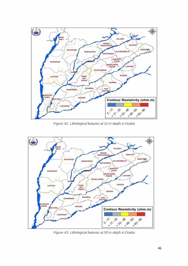
46
Figure 42. Lithological features at 10 m depth in Doabs
Figure 43. Lithological features at 50 m depth in Doabs

47
Soil Organic Matter in Pothwar
Organic matter has direct bearing on infiltration and soil moisture-retention
characteristics of soil. Figures 44 to 46 shows spatial and up to 1.0 m depth
distribution of organic matter in Pothwar, while Table 6 shows percent areas of
all three layers of the region having different values of organic matter. The values
vary from 0.2 to 2.5%. The highest organic matter is in the surface layer at the
Himalayan piedmont where rainfall and vegetative cover are normally higher than
the other areas.
Qureshi et al. (2000) found organic matter of 0.25-0.8% in Tehsil Gujar Khan.
Figure 44 shows decreasing trend of organic matter towards Gujar Khan area.
The organic matter also decreases with depth. The lowest organic matter both at
the surface and up to 1.0 m depth are in the south-west region, where vegetation
is sparse owing to low rainfall. Organic matter in the deep soil is only due to decay
of plant roots. Therefore, organic matter decreases with depth and the trend
prevails over the entire region.
Table 6. Pothwar region having different values of organic matter (%)
Organic Matter
(%)
Percent Area
(Surface
Layer)
Percent Area
(Middle Layer)
Percent Area
(Bottom
Layer)
0.20 to 0.50 2.80 4.70 15.80
0.50 to 0.75 15.10 23.90 36.50
0.75 to 1.00 21.20 49.30 37.10
1.00 to 1.50 42.80 21.50 10.60
1.50 to 2.00 15.80 0.60 0.10
2.00 to 2.50 2.40 0.00 0.00
Total 100 100 100

48
Figure 44. Spatial distribution of soil organic matter in surface layer of Pothwar
Figure 45. Spatial distribution of soil organic matter in middle layer of Pothwar

49
Figure 46. Spatial distribution of soil organic matter in bottom layer of Pothwar
Chemical Properties of Pothwar Soils
Electrical conductivity of the saturated paste measured at standard temperature
of 25 oC gives an index of the salinity status of the soil. According to US standard,
EC<4 dS/m is of normal soil and above 4 dS/m have various degrees of salinity.
Soils having SAR greater than 13 associated with pH>8.5 are called sodic soils.
Soils may be saline, sodic or saline sodic. A saline soil may not necessarily be
sodic. In the past, the term alkali and sodic soils were considered synonymous.
However, the term refers peculiarly to excess of sodium, whereas pH may be
high with or without high sodium content. In other words, a soil high in sodium
contents should have pH>8.5 as well but a soil having high pH does not
necessarily contain excessive sodium. The soils having pH>8.5 without SAR
beyond the admissible limit of 13 are preferably called alkali soils (Reed and
Soreston, 1997). However, a soil having SAR less than 13 but with high Mg
contents may have serious concerns (Yadav and Girdhar, 1981; Qadir and
Schubert, 2002; Qadir and Oster, 2004).
Mapping of EC values of soil samples taken from surface, 0.5 and 1.0 m depths
in Pothwar are given in Figures 47 to 49, respectively. The EC values are below
2 dS/m in most of the areas and within the admissible value in the entire area
except at a few patches. The site of EC value of the highest range (>8 dS/m) is

50
in Rawalpindi district on Chakbelli Road some 25 km off GT Road towards
Chakwal. This area falls in the region of appreciable rain above 600 mm.
Therefore, the spot values of salinity might be result of saline seeps. Saline soil
spots due to saline seep develop on undulating soils where shallow permeable
soil is underlain by impermeable rocks. Horizontal movement of infiltrated water
under such conditions remain dominant due to impeding layer underneath. The
horizontal movement of water carries soluble salts from upslope towards
depressions. Water evaporates from depression and saline spots are formed
(Miller et al., 1981). This phenomenon may be observed at large as well as
smaller scales. Pothwar is prone to saline seep spots owing to its peculiar
topography, and shallow soils. However, EC values over 4 dS/m in Attock area
is quite possible owing to barren tract falling out of monsoon belt. On the overall
basis, EC values are well within admissible range and decease with increase in
depth to 1.0 m especially in Gujar Khan area, which are supported by the results
presented by Shaheen (2016). The Site-2, where EC in the surface layer falls in
the range 4-8 dS/m, is close to Taxila. This has also been reported by Fateh et
al., (2006).
Figure 47. The EC in the surface layer

51
Figure 48. The EC in the middle (0.5 m depth) layer
Figure 49. The EC in the bottom (1.0 m depth) layer

52
Sodium absorption ratio (SAR) for surface, middle (0.5 m) and bottom (1.0 m)
layers of the study are given in Figures 50 to 52, respectively. SAR values are
within admissible range except at few patches.
In general, there is no sodicity hazard in Pothwar but salinity exist in patches due
to apparent reason of saline seeps. Saline seepage accumulation in low-lying
area impeded by impermeable layer may be a peculiar phenomenon in Pothwar
where land is highly undulated, dissected and outcropped. Such phenomenon is
more dominant in shallow and permeable soils falling in appreciable rainfall area,
fallow soils and the soils that have been overgrazed, deforested or devoid of
vegetation (Abrol et al., 1988). Since Pothwar is rain-fed rea, secondary salination
due to brackish irrigation water is not expected. Main source of salts in such soils
are due to constituent minerals, which undergo series of changes involving
weathering, oxidation, hydration, hydrolysis and carbonation etc. that make the
salts soluble thereby making them available for transportation with water (Abrol
et al., 1988). None of the surveyed sites fall near Kallar Kahar lake which serves
as a closed basin where salinity level could be more than elsewhere due to
washing of salts with runoff from upslopes (Ashraf et al., 2012).
Although salinity is sparse and sodicity is almost non-existent in the Pothwar
region, pH mappings (Figures 53 to 55) show that it casually goes beyond 8.4 in
all the three layers. Sodic soils are supposed to have higher value of pH. As
stated elsewhere, soils having higher values of pH are not necessarily sodic but
are called alkali soils (Reed and Sorensen, 1997).
Site-17 located near Khurd, on Pind Dadan Khan-Jhelum road has persistently
higher value of pH in middle and bottom layers, whereas the same site shows
increasing values of SAR with depth and exceeded beyond the admissible range
at the bottom layer. Being in the salt range, this area has inherent tendency of
sodicity owing to its parent material and therefore, have higher values of SAR
and pH.
It is pertinent to mention that in our case carbonate was persistently below
detection limit (5 ppm) at almost all the sites and therefore, Residual Sodium
Carbonate (RSC) remained undetermined, as the resulting value was negative.
It can be safely concluded that no appreciable salinity or sodicity hazard is
available in Pothwar except sparse salinity patches.

53
Figure 50. SAR in surface layer
Figure 51. SAR in the middle (0.5 m depth) layer
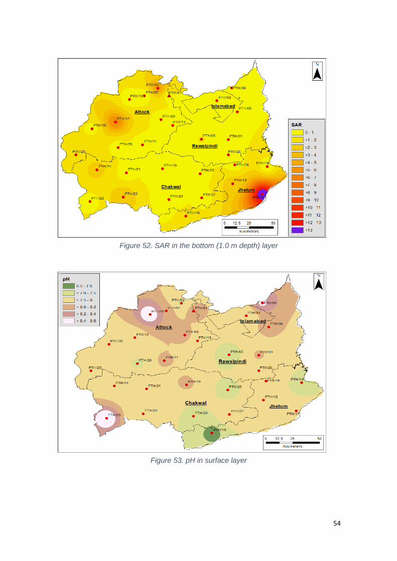
54
Figure 52. SAR in the bottom (1.0 m depth) layer
Figure 53. pH in surface layer

55
Figure 54. pH in the middle (0.5 m depth) layer of Pothwar
Figure 55. pH in the bottom (1.0 m depth) layer

56
7. Conclusions
The study provides soil hydraulic and physical properties for Pothwar and Doabs
in Punjab province. Cumulative infiltration data of infiltration tests yielded less
scatter due to compensation of random error in the cumulative infiltration,
whereas incremental point infiltration rates data reflects more scatter resulting in
unimpressive goodness of fit in terms of R2. Horton’s cumulative infiltration model
persistently fits better or comparable to the Philip’s model in terms of R2 as
goodness of fit. Horton’s infiltration model gives direct estimate of steady-state
infiltration rates, which is very often required as practical equivalence of field
saturated conductivity, whereas it is difficult to acquire the same by using Philip’s
model.
Sandy loam, loam and silt loam are dominant soil textural classes in Pothwar and
Doabs. However, spatial coverage of sandy loam decreases with depth in the
Pothwar region, whereas clay fraction decreases with depth in the Doab’s.
Moisture-retention characteristics are more variable for similar classes of soil in
the Pothwar Region than in Doabs.
The soil with infiltration rates up to 45 mm/hr are dominant in the Pothwar,
whereas soil with infiltration rates up to 30 mm/hr are dominant in Doabs.
Lithological strata are more diverse in Pothwar Region as compared to Doabs
where it is almost uniform. Soil organic matter contents in the Pothwar vary from
0.2 to 2.5%. The highest percentage is found in the northern piedmonts and the
lowest in the southern parts. There are no hazards of sodicity and or salinity in
the Pothwar region.

57
References
Abdulkadir, A., M.N. Wuddivira, N. Abdu and O. J. Mudiare (2011). Use of Horton
infiltration model in estimating infiltration characteristics of an Alfisol in the
Northern Guini Savana of Nigeria. Journal of Agricultural Science and
Technology, A1, 925-931.
Abrol, I.P., J.S.P. Yadav, and F.I, Massound (1998). Salt-affected soils and their
management. FAO Soil Resources and Conservation Services, Land
Water Development Division, FAO Soils Bulletin 39, FAO of United
Nations, Room.
Ashraf, M., T. Oweis, A. Razzaq, B. Hussain and A. Majid (2012). Spatial and
temporal analysis of water quality in the Dharbi watershed of Pakistan:
issues and options. Journal of Environmental Sciences and Engineering,
A. 1:329-340.
Batkova, K., S. Matula., Mihalikov and, M. (2013). Study guide of field
hydrological measurement. 2nd edition (on-line). English version. Czech
University of Life Sciences Prague. Prague, Czech Republic. Available at:
http://hydropedologie. Agrobiologie.cz. ISBN: 978-80-213-2434-3.
Bevin, K.J., (2004). Robert E. Horton’s perceptual model of infiltration processes.
Hydrological Processes 18: 3447-3460.
Bouma, J. (1989). Using soil survey data for quantitative land
evaluation. Advances in Soil Science. 9: 177–213.
Childs, E.C. and M. Bybordi. (1969). The vertical movement of water in stratified
porous material. 1. Infiltration. Water Resources Research, 5(2), 446-459.
Doneen, L.D. and D.W. Wescot (1988). Irrigation management practices, based
on FAO Irrigation and Drainage Paper 1, Oxford and IB Publishing Co. Pvt
Ltd, New Delhi.
Fateh, S., M. Arshad, M.A. Naeem and M.I. Latif (2006). Physio-chemical
characteristics of soils of Poth war and determination of organic matter.
Pakistan Journal of Biological Sciences. 9 (3): 473-476.
Gohardoust, M.R., M. Sadeghi, M.Z. Ahmadi, S.B. Jones and M. Tuller (2017).
Hydraulic conductivity of stratified unsaturated soils: Effects of random
variability and layering. Journal of Hydrology 546:81-89.
Green, W.H. and G. Ampt. (1911). Studies on Soil Physics. The Journal of
Agricultural Science. 4: 1.

58
Haverkamp, R., L. Rendon and G. Vachaud (1987). Infiltration equations and their
applicability for predictive use. P. 142-152. In Yu- SI Fok (ed.) Infiltration
Development and Application. Honolulu, Hawaii.
Hillel, D. (1982). Introduction to Soil Physics, Academic Press Inc, London.
Hillel, D. and W.R. Gardner (1970). Transient infiltration into crust topped profiles.
Soil Science, 109: 69-76.
Horton, R. E. (1940). An approach toward a physical interpretation of infiltration
capacity. Proc. Soil Sci. Soc. Amer. 5: 399-417.
Khan, A.D., N. Iqbal, M. Ashraf, and A.A. Sheikh (2016). Groundwater
Investigation and Mapping the Upper Indus Plain, Pakistan Council of
Research in Water Resources, Islamabad.
Kirsch, T.D., C. Wadhwani, L. Sauer, S. Doocy, and C. Catlett (2012). Impact of
the 2010 Pakistan floods on rural and urban populations at six Months.
PLOS Currents Disasters. 2012 Aug 22. Edition 1.
Kostiakov, A. N. (1932). The dynamics of the coefficients of water percolation in
soils and the necessity for studying it from a dynamic point of view for
purpose of amelioration. Society of Soil Sci., 14: 17-21.
Lin, H., J. Bouma, L.P. Wilding, J.L. Richardson, M. Kutílek and D.R. Nielsen
(2005). Advances in hydropedology. Advances in Agronomy, 851-8..
https://doi.org/10.1016/S0065-2113(04)85001-6
Malik, M.A. and M. Ashraf (2017). Determining river basin hydraulic and physical
characteristics: A Manual. Pakistan Council of Research in Water
Resources (PCRWR), pp. 88.
Miller, M., P. Brown, J. Donovan, R. Bergatino, J. Sonderegger and F. Schmidt
(1981). Saline seep development and control in the North American Great
Plains - Hydroceological Aspects. Developments in Agricultural
Engineering Land and Stream Salinity, 115-141.
Naeth, M. A. (1988). The impact of grazing on litter and hydrology in mixed prairie
and fescue grassland ecosystems of Alberta. Ph.D. Thesis. University of
Alberta, Edmonton, Canada.
Philip, J.R. (1957). The Theory of Infiltration-1, The Infiltration equation and its
solution, Soil Sci., 83: 345-357.
Philip, J.R. (1969). Hydrostatics and hydrodynamics in swelling soils. Water
Resources Research, 5(5), 1070-1077.

59
Qadir, M. and S. Schubert. (2002). Degradation processes and nutrient
constraints in sodic soils. Land Degrad. Develop., 13: 275-294.
Qadir, M., J.D. Oster (2004). Crop and irrigation management strategies for
saline-sodic soils and waters aimed at environmentally sustainable
agriculture. Science of the Total Environment, 323, 1-19.
Qureshi, S.J., A. Rizwana, A. Qureshi, M. Yousuf and M. Rizwan (2000). Organic
Matter xtacts of Gujar Khan Tehsil. Pakistan Journal of Biological
Sciences: 3 (12): 2033-2034.
Reed, P.E. and C.J. Sorenson (1997). Potential for sodium and salinity in the soil-
survey mapping units of Kansas. Department of Geography, University of
Kensas, USA.
Richard, A.J. and G.F. Gifford (1981). An In-Depth Examination of the Philip
Equation for Cataloging Infiltration Characteristics in Rangeland
Environments. Journal of Range Management: 34(4).
Richards, L. A. (1931). Capillary conduction through porous mediums. Physics 1:
313-318.
Shaheen, A. (2016). Characterization of eroded lands of Pothwar plateau,
Punjab, Pakistan. Sarhad Journal of Agriculture, 32(3): 192-201.
Sheikh, A.A., M. Ashraf and A. Bahzad (2007). Assessment of water resources
and development of strategic water utilization plan in Pothwar Region for
its sustainable management. Research Report 7-2007, Pakistan Council
of Research in Water Resources, Ministry of Science and Technology,
Islamabad, Pakistan.
Telis, P.A. (2001). Estimation of infiltration rates of saturated soils at selected
sites in the Caloosahatchee River Basin. Southwestern Florida, U.S.
Geological Survey, Open-File Report 01-65 Prepared in cooperation with
the South Florida Water Management District.
Turner, E. (2006). Comparison of infiltration equations and their validation with
rainfall simulation. M.Sc. Thesis, Department of Biological Resources
Engineering, Faculty of the Graduate School of the University of Maryland,
College Park.
Van Genuchten, M.T. (1980). A closed-form equation for predicting the Hydraulic
Conductivity of Unsaturated Soils. Soil Sci. Soc. Am. J.44: 892-898.
Warrick, A.W. (2005). Effective unsaturated hydraulic conductivity for one-
dimensional structured heterogeneity. Water Resources Research, 41(9).

60
Yadav, J. S., & Girdhar, I.K. (1981). The Effects of different magnesium: calcium
ratios and sodium adsorption ratio values of leaching water on the
properties of calcareous versus noncalcareous soils. Soil Science, 131(3),
194.
Zhu, J. (2008). Equivalent parallel and perpendicular unsaturated hydraulic
conductivities: Arithmetic Mean or Harmonic Mean? Soil Science Society
of America Journal: 72(5).
Zhu, J. and A.W. Warrick (2012). Unsaturated hydraulic conductivity of repeatedly
layered Soil Structures. Soil Science Society of America Journal:
76(1):28.

61
Annexure - A (Pothwar and Doabs Dataset)
Pothwar
Horton Model Results
(Fitting on Cumm. Infil.)
ϴs
(cm3/cm
3)
ϴr
(cm3/cm
3)
α
(cm-1
)n
S
(mm/hr1/2
)
A (mm/hr)
Infil. Rate
4 hr (mm/hr)
Infil. Rate
8 hr (mm/hr)
fc (mm/hr)Clay
(%)
Silt
(%)
Sand
(%)Soil Type
S 0.459 0.097 0.009 1.398 23.42 0.006 4.43 4.15 7.80 21.1 58.0 20.9 Silt Loam 1.55
M 0.446 0.020 0.007 1.217 21.52 2.032 6.10 5.84 9.97 25.1 58.0 16.9 Silt Loam 1.58
B 0.474 0.030 0.023 1.281 22.13 1.576 5.76 5.49 10.36 21.1 62.0 16.9 Silt Loam 1.36
S 0.520 0.172 0.007 1.322 9.19 0.006 2.30 1.63 1.81 37.0 44.0 19.0 Silty Clay Loam 1.66
M 0.476 0.020 0.001 1.247 4.76 0.006 1.13 0.85 0.85 43.0 36.0 21.0 Clay 1.63
B 0.473 0.269 0.006 3.622 16.68 6.398 10.57 9.35 13.24 27.0 15.5 57.5 Sandy Clay Loam 1.56
S 0.439 0.020 0.141 1.086 9.62 1.061 3.47 2.76 4.74 23.5 50.0 26.5 Silt Loam 1.68
M 0.470 0.020 0.022 1.161 11.21 24.330 27.13 26.31 28.11 21.5 24.7 53.8 Sandy Clay Loam 1.77
B 0.417 0.211 0.021 1.644 22.90 0.825 6.55 4.87 10.58 23.5 36.0 40.5 Loam 1.57
S 0.350 0.132 0.010 1.625 13.17 0.006 3.30 2.33 4.29 7.7 35.3 57.0 Sandy Loam 1.78
M 0.366 0.123 0.018 1.502 1.58 10.574 10.97 10.85 11.30 10.7 21.7 67.7 Sandy Loam 1.83
B 0.374 0.020 0.033 1.168 5.74 1.853 3.29 2.87 4.48 13.7 29.3 57.0 Sandy Loam 1.84
S 0.386 0.102 0.019 1.527 14.08 62.828 66.35 65.32 68.11 17.1 20.7 62.2 Sandy Loam 1.66
M 0.433 0.093 0.028 1.937 6.87 67.159 68.88 68.37 69.94 11.1 18.7 70.2 Sandy Loam 1.50
B 0.389 0.096 0.016 1.716 24.12 17.493 23.52 21.76 26.44 13.1 18.7 68.2 Sandy Loam 1.63
S 0.412 0.020 0.012 1.217 33.94 0.006 8.49 6.01 14.23 15.0 30.0 55.0 Sandy Loam 1.74
M 0.368 0.081 0.019 1.966 37.34 31.162 40.50 37.76 49.22 9.0 17.3 73.7 Sandy Loam 1.66
B 0.360 0.083 0.030 2.268 13.31 44.267 47.60 46.62 50.72 5.0 9.3 85.7 Loamy Sand 1.63
S 0.410 0.078 0.013 1.184 5.36 0.006 1.35 0.95 0.22 15.0 46.0 39.0 Loam 1.70
M 0.468 0.153 0.008 1.642 43.72 9.187 20.12 16.92 26.04 7.0 45.3 47.7 Loam 1.58
B 0.475 0.176 0.009 1.465 21.92 0.983 6.46 4.86 9.05 13.0 42.7 44.4 Loam 1.51
S 0.438 0.072 0.006 1.504 22.45 7.175 12.79 11.14 15.89 16.2 67.9 15.8 Silt Loam 1.57
M 0.474 0.088 0.018 1.335 50.29 0.006 12.58 8.90 18.23 24.2 61.3 14.5 Silt Loam 1.41
B 0.472 0.110 0.016 1.388 32.14 7.609 15.64 13.29 19.74 20.2 63.9 15.8 Silt Loam 1.54
S 0.390 0.020 0.016 1.054 21.96 0.006 5.50 3.89 2.70 17.7 47.3 35.0 Loam 1.66
M 0.402 0.020 0.009 1.147 11.24 0.006 2.81 1.99 3.78 35.7 10.7 53.7 Sandy Clay 1.73
B 0.325 0.087 0.006 1.099 4.71 0.006 1.18 0.84 0.58 33.7 28.0 38.3 Clay Loam 1.86
S 0.479 0.113 0.035 1.376 20.79 43.933 49.13 47.61 51.79 5.5 42.7 51.8 Sandy Loam 1.20
M 0.441 0.244 0.017 1.368 12.48 10.241 13.36 12.45 14.98 23.5 42.7 33.8 Loam 1.60
B 0.357 0.042 0.025 1.093 23.45 3.246 9.11 7.39 11.92 23.5 40.7 35.8 Loam 1.66
PTH/01 33.7477 72.7069
PTH/02 33.8239 72.6039
Site
No.Lat. Long.
L
a
y
e
r
Moisture Retention ParametersPhilips Model Results
(Fitting on Cumm. Infil.)Soil texture
Bulk
Density
(g/cm3)
PTH/05 33.3299 73.0036
PTH/06 33.5961 73.3339
PTH/03 33.3264 73.2508
PTH/04 33.7028 73.1453
PTH/09 33.8258 73.2811
PTH/10 33.7158 72.3428
PTH/07 33.7497 72.4786
PTH/08 33.5197 72.6319

62
Pothwar
Horton Model Results
(Fitting on Cumm. Infil.)
ϴs
(cm3/cm
3)
ϴr
(cm3/cm
3)
α
(cm-1
)n
S
(mm/hr1/2
)
A (mm/hr)
Infil. Rate
4 hr (mm/hr)
Infil. Rate
8 hr (mm/hr)
fc (mm/hr)Clay
(%)
Silt
(%)
Sand
(%)Soil Type
S 0.362 0.259 0.009 1.380 4.95 110.011 122.39 118.76 129.85 22.2 33.3 44.4 Loam 1.83
M 0.404 0.020 0.008 1.096 0.76 0.006 1.91 1.35 1.69 28.2 30.0 41.8 Clay Loam 1.75
B 0.391 0.212 0.005 1.322 0.70 0.006 1.75 1.24 0.11 22.2 24.7 53.1 Sandy Clay Loam 1.85
S 0.394 0.158 0.029 1.387 0.69 0.538 2.25 1.75 3.14 21.0 41.3 37.7 Loam 1.76
M 0.405 0.101 0.018 1.309 1.68 17.108 21.32 20.09 23.78 23.0 45.3 31.7 Loam 1.58
B 0.431 0.116 0.018 1.571 5.64 22.755 36.86 32.73 42.08 19.0 42.7 38.4 Loam 1.51
S 0.378 0.099 0.014 1.445 1.59 0.006 3.97 2.81 3.80 14.2 32.7 53.1 Sandy Loam 1.65
M 0.359 0.020 0.037 1.087 2.08 0.432 5.63 4.11 8.28 34.2 35.3 30.4 Clay Loam 1.87
B 0.319 0.020 0.018 1.104 1.00 0.006 2.51 1.78 3.11 34.2 48.0 17.8 Silty Clay Loam 1.88
S 0.382 0.114 0.021 2.206 0.03 45.906 45.97 45.95 45.85 3.1 24.7 72.2 Sandy Loam 1.70
M 0.374 0.036 0.045 1.239 1.75 44.016 48.39 47.11 50.51 13.1 32.0 52.9 Sandy Loam 1.69
B 0.369 0.070 0.024 1.361 5.70 51.515 65.77 61.59 73.32 23.1 16.7 60.2 Sandy Clay Loam 1.70
S 0.413 0.064 0.008 1.327 1.42 9.006 12.56 11.52 14.50 11.1 61.3 27.6 Silt Loam 1.71
M 0.478 0.020 0.014 1.326 3.76 14.533 23.93 21.17 27.34 13.1 65.3 21.6 Silt Loam 1.49
B 0.473 0.020 0.028 1.232 3.13 6.789 14.63 12.33 17.85 21.1 62.7 16.2 Silt Loam 1.41
S 0.404 0.105 0.021 2.623 1.11 56.753 59.54 58.72 61.15 9.1 11.3 79.6 Silt Loam 1.72
M 0.374 0.020 0.032 1.186 1.52 54.649 58.44 57.33 59.56 15.2 16.6 68.3 Sandy Loam 1.74
B 0.366 0.020 0.023 1.190 1.11 56.753 59.54 58.72 30.37 13.1 65.6 21.3 Silt Loam 1.74
S 0.495 0.020 0.002 1.218 1.57 11.785 15.72 14.57 17.66 26.4 36.0 37.6 Loam 1.53
M 0.379 0.020 0.010 1.274 1.32 0.957 4.25 3.29 6.06 9.1 42.0 48.9 Loam 1.83
B 0.432 0.020 0.003 1.390 2.16 0.006 5.40 3.82 3.86 12.4 69.3 18.3 Silt Loam 1.63
S 0.381 0.024 0.034 1.286 2.80 31.468 38.47 36.42 42.54 13.7 38.7 47.7 Loam 1.60
M 0.455 0.024 0.015 1.358 2.71 6.030 12.80 10.82 16.48 15.7 56.7 27.7 Silt Loam 1.55
B 0.430 0.091 0.038 1.213 3.70 3.852 13.10 10.39 16.24 35.7 43.3 21.0 Clay Loam 1.59
S 0.381 0.024 0.034 1.286 1.24 16.922 20.01 19.11 21.90 23.7 54.0 22.3 Silt Loam 1.73
M 0.455 0.024 0.015 1.358 4.08 86.618 96.81 93.82 101.89 23.7 39.3 37.0 Loam 1.52
B 0.429 0.020 0.032 1.179 3.50 52.807 61.56 59.01 61.98 21.7 56.0 22.3 Silt Loam 1.34
S 0.383 0.078 0.018 1.607 2.15 0.006 3.80 3.80 6.95 5.8 20.7 73.5 Sandy Loam 1.71
M 0.400 0.089 0.019 1.832 3.46 89.381 98.04 95.50 103.37 7.8 21.3 70.8 Sandy Loam 1.48
B 0.384 0.060 0.028 1.456 4.19 43.261 53.73 50.67 58.60 11.8 17.3 70.8 Sandy Loam 1.35
PTH/11 33.2753 72.4614
PTH/12 33.4953 72.2144
Site
No.Lat. Long.
L
a
y
e
r
Moisture Retention ParametersPhilips Model Results
(Fitting on Cumm. Infil.)Soil texture
Bulk
Density
(g/cm3)
PTH/15 32.8992 73.2903
PTH/16 33.0808 73.3106
PTH/13 33.4639 72.7400
PTH/14 33.0661 73.6078
PTH/19 33.0606 72.6467
PTH/20 32.7443 72.7048
PTH/17 32.7961 73.5647
PTH/18 32.5847 72.8600

63
Pothwar
Horton Model Results
(Fitting on Cumm. Infil.)
ϴs
(cm3/cm
3)
ϴr
(cm3/cm
3)
α
(cm-1
)n
S
(mm/hr1/2
)
A (mm/hr)
Infil. Rate
4 hr (mm/hr)
Infil. Rate
8 hr (mm/hr)
fc (mm/hr)Clay
(%)
Silt
(%)
Sand
(%)Soil Type
S 0.434 0.125 0.042 1.220 13.62 2.071 5.47 4.47 7.22 29.8 32.7 37.5 Clay Loam 1.67
M 0.470 0.209 0.033 1.261 35.31 0.006 8.83 6.24 10.07 41.8 32.7 25.5 Clay 1.60
B 0.445 0.189 0.013 1.390 48.04 0.005 12.01 8.49 14.67 21.8 42.7 35.5 Loam 1.62
S 0.415 0.050 0.023 1.217 38.32 4.855 14.43 11.62 18.86 17.8 52.0 30.2 Silt Loam 1.57
M 0.389 0.020 0.022 1.124 12.95 0.006 3.34 2.29 0.63 11.8 69.3 18.8 Silt Loam 1.65
B 0.385 0.020 0.018 1.156 8.28 0.006 2.07 1.46 2.13 3.8 54.7 41.5 Silt Loam 1.65
S 0.367 0.127 0.023 1.746 33.20 79.467 87.77 85.33 91.82 7.8 15.3 76.8 Sandy Loam 1.62
M 0.462 0.100 0.008 1.962 7.03 28.300 30.05 29.54 31.20 5.8 32.7 61.5 Sandy Loam 1.56
B 0.461 0.020 0.007 1.268 7.43 31.172 33.02 32.48 34.27 31.8 54.7 13.5 Silty Clay Loam 1.56
S 0.359 0.025 0.042 1.236 18.51 33.094 37.72 36.36 42.53 11.8 26.7 61.5 Sandy Loam 1.70
M 0.397 0.068 0.019 3.938 0.00 313.260 313.26 313.26 16.47 0.0 8.0 92.0 Sand 1.58
B 0.389 0.048 0.027 2.894 174.66 193.169 236.84 224.04 16.23 0.0 3.0 97.0 Sand 1.62
S 0.418 0.114 0.013 1.383 26.57 29.567 20.01 19.11 39.87 17.8 27.3 54.8 Sandy Loam 1.39
M 0.416 0.020 0.019 1.191 22.47 38.460 96.81 93.82 46.70 23.8 54.7 21.5 Silt Loam 1.48
B 0.451 0.171 0.035 1.486 50.25 7.290 61.56 59.00 26.80 27.8 54.0 18.2 Silty Clay Loam 1.43
S 0.456 0.032 0.028 1.222 9.09 0.006 2.28 1.61 1.32 15.8 52.7 31.5 Silt Loam 1.44
M 0.372 0.020 0.004 1.244 20.65 23.623 28.79 27.27 31.51 19.8 44.0 36.2 Loam 1.68
B 0.473 0.020 0.012 1.296 15.13 7.542 11.32 10.22 13.47 13.8 54.7 31.5 Silt Loam 1.49
S 0.506 0.332 0.054 1.320 37.89 43.221 52.69 49.92 56.08 31.8 41.3 26.8 Clay Loam 1.27
M 0.445 0.020 0.006 1.084 11.96 2.215 5.20 4.33 6.77 33.8 39.3 26.8 Clay Loam 1.36
B 0.464 0.047 0.043 1.043 4.64 0.006 1.17 0.83 0.00 27.8 35.3 36.8 Clay Loam 1.49
S 0.383 0.082 0.024 1.950 38.18 82.735 92.28 89.48 97.68 8.6 16.7 74.8 Sandy Loam 1.50
M 0.389 0.069 0.022 2.393 41.14 195.766 206.05 203.04 211.56 2.6 22.0 75.4 Loamy Sand 1.41
B 0.365 0.067 0.019 1.695 58.97 129.241 143.98 139.67 151.40 6.6 21.3 72.1 Sandy Loam 1.51
S 0.425 0.020 0.045 1.150 13.35 12.325 15.66 14.69 17.52 28.6 20.0 51.4 Sandy Clay Loam 1.40
M 0.458 0.175 0.072 1.735 120.44 54.655 84.76 75.95 101.51 20.6 17.3 62.1 Sandy Clay Loam 1.37
B 0.431 0.148 0.071 1.583 107.04 16.313 43.07 35.24 56.95 14.6 17.3 68.1 Sandy Loam 1.41
S 0.398 0.050 0.046 2.360 184.11 222.824 268.85 255.37 42.08 0.0 6.0 94.0 Sand 1.65
M 0.348 0.086 0.045 2.027 337.16 195.904 280.19 255.51 312.11 3.8 9.3 86.9 Sand 1.55
B 0.368 0.089 0.052 2.077 176.84 128.058 172.27 159.32 194.13 5.1 9.3 85.5 Loamy Sand 1.49
Site
No.Lat. Long.
L
a
y
e
r
Moisture Retention ParametersPhilips Model Results
(Fitting on Cumm. Infil.)Soil texture Bulk
Density
(g/cm3)
PTH/23 32.7258 71.9794
PTH/24 33.0326 72.0436
PTH/21 33.0051 72.3143
PTH/22 32.7686 72.2860
PTH/27 32.7616 73.0055
PTH/28 33.2479 72.2372
PTH/25 32.9949 72.9915
PTH/26 33.1778 73.2518
PTH/29 33.1782 71.8496
PTH/30 33.4315 71.9986
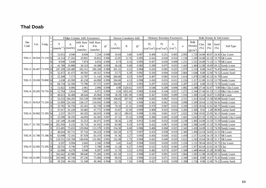
64
Thal Doab
S 15.015 4.940 8.694 7.234 0.998 10.04 3.80 0.997 0.468 0.251 0.005 2.092 1.720 34.88 40.67 24.45 Clay Loam
M 14.154 17.263 20.801 18.852 0.996 22.85 12.76 0.995 0.424 0.020 0.016 1.136 1.549 16.88 63.33 19.79 Silt Loam
B 8.938 5.640 7.874 6.816 0.996 8.74 4.16 0.995 0.457 0.020 0.008 1.231 1.551 16.88 71.33 11.79 Silt Loam
S 41.780 19.888 30.333 34.388 0.993 36.24 9.49 0.985 0.399 0.075 0.033 1.443 1.484 12.88 18.00 69.12 Sandy Loam
M 247.299 120.486 182.311 206.168 0.989 201.31 4.23 0.984 0.418 0.082 0.025 1.979 1.510 8.88 14.67 76.45 Sandy Loam
B 32.472 41.473 49.591 44.351 0.994 53.75 6.39 0.992 0.350 0.094 0.020 2.864 1.648 8.88 12.00 79.12 Loamy Sand
S 22.449 7.175 12.787 11.143 0.996 284.80 4.53 0.997 0.407 0.082 0.013 1.614 1.476 12.88 45.33 41.79 Loam
M 5.038 43.999 45.258 44.890 0.999 284.80 4.53 0.998 0.450 0.035 0.012 2.224 1.317 12.88 33.33 53.79 Sandy Loam
B 84.734 52.596 73.780 67.575 0.997 284.80 4.53 0.993 0.297 0.025 0.019 2.287 1.325 6.88 19.33 73.79 Sandy Loam
S 11.822 0.006 2.961 2.096 0.999 4.98 1529.61 0.957 0.548 0.208 0.006 1.882 1.348 27.44 62.67 9.89 Silty Clay Loam
M 12.764 3.814 7.005 6.071 0.999 9.20 1052.45 0.983 0.434 0.144 0.021 1.272 1.544 27.44 61.33 11.23 Silty Clay Loam
B 48.623 36.488 48.644 45.084 0.996 58.29 1381.90 0.985 0.367 0.092 0.009 1.916 1.369 13.44 54.67 31.89 Silt Loam
S 33.333 184.205 192.539 190.098 0.999 196.84 287.93 0.999 0.445 0.062 0.014 2.551 1.414 16.64 15.28 68.08 Sandy Loam
M 55.809 124.184 138.137 134.050 0.998 145.71 17.81 0.999 0.361 0.061 0.016 3.098 1.509 18.64 11.95 69.41 Sandy Loam
B 33.782 56.756 65.201 62.728 0.998 70.10 21.31 0.999 0.370 0.067 0.013 3.169 1.535 18.64 12.61 68.75 Sandy Loam
S 37.017 41.228 50.482 47.772 0.996 55.87 32.50 0.999 0.408 0.025 0.034 3.283 1.366 9.92 1.28 88.80 Loamy Sand
M 2.537 59.571 60.205 60.019 0.998 60.12 180.63 0.998 0.336 0.061 0.017 2.022 1.594 19.92 23.95 56.13 Sandy Loam
B 23.590 38.195 44.093 42.365 0.997 47.31 19.16 0.999 0.380 0.065 0.020 1.601 1.645 21.92 15.95 62.13 Sandy Clay Loam
S 147.249 18.440 55.253 44.471 0.995 58.26 2.29 0.953 0.436 0.032 0.020 2.238 1.485 14.08 13.33 72.59 Sandy Loam
M 201.950 6.232 56.719 41.932 0.995 83.90 9.19 0.979 0.432 0.067 0.019 2.560 1.586 14.08 15.33 70.59 Sandy Loam
B 213.405 75.653 129.004 113.378 0.995 154.30 6.60 0.986 0.408 0.068 0.025 2.342 1.439 14.08 11.33 74.59 Sandy Loam
S 48.044 85.731 97.742 94.224 0.998 102.50 4.75 0.997 0.435 0.058 0.018 2.360 1.496 22.64 54.85 22.51 Silt Loam
M 63.098 72.165 87.939 83.319 0.994 91.36 3.27 0.993 0.456 0.020 0.022 1.418 1.517 12.64 54.19 33.17 Silt Loam
B 119.551 110.768 140.656 131.902 0.991 132.49 1.75 0.994 0.425 0.040 0.019 1.612 1.545 10.64 58.19 31.17 Silt Loam
S 6.597 0.994 2.643 2.160 0.998 3.41 6.62 0.994 0.635 0.020 0.055 1.224 1.131 38.64 28.61 32.75 Clay Loam
M 28.555 0.740 7.879 5.788 0.996 11.24 6.27 0.995 0.525 0.055 0.043 1.470 1.357 42.64 22.61 34.75 Clay
B 22.680 4.278 9.948 8.287 0.997 11.70 3.51 0.995 0.482 0.073 0.037 1.508 1.449 44.64 25.28 30.08 Clay
S 182.642 42.980 88.640 75.266 0.995 101.50 3.31 0.998 0.447 0.091 0.015 1.864 1.585 12.88 18.00 69.12 Sandy Loam
M 165.960 45.746 87.236 75.084 0.994 90.03 2.24 0.996 0.524 0.071 0.013 2.349 1.663 8.88 14.67 76.45 Sandy Loam
B 29.250 44.195 51.508 49.366 0.994 55.39 7.16 0.993 0.427 0.033 0.039 1.398 1.756 8.88 12.00 79.12 Loamy Sand
Philips Commu. Infil. Parameters Horton Comulative Infil. Moisture Retention Parameters Bulk Density & Soil texture
S
(mm/hr1/2
)Soil Type
Site
CodeLat. Long.
L
a
y
e
r
THL/2 30.467 71.078
THL/3 29.658 70.800
Clay
(%)
Silt
(%)
Sand
(%)
THL/1 30.024 71.119
R2
ϴs
(cm3/cm
3)
ϴr
(cm3/cm
3)
α
(cm-1
)n
Bulk
Density
(g/cm3)
A
(mm/hr)
Infil. Rate
4 hr
(mm/hr)
Infil. Rate
8 hr
(mm/hr)
R2
Fc
(mm/hr)K
THL/6 30.892 71.595
THL/7 31.782 72.049
THL/4 29.205 70.755
THL/5 30.814 71.216
THL/10 32.085 71.613
THL/8 31.786 71.186
THL/9 32.092 71.295

65
Thal Doab
S 82.641 18.745 39.405 33.354 0.997 50.25 8.42 0.984 0.467 0.073 0.021 1.735 1.385 12.88 18.00 69.12 Sandy Loam
M 169.382 40.259 82.604 70.201 0.995 87.82 2.36 0.997 0.459 0.051 0.022 2.617 1.572 8.88 14.67 76.45 Sandy Loam
B 31.157 41.999 49.789 47.507 0.993 53.95 7.22 0.991 0.492 0.044 0.023 3.064 1.465 8.88 12.00 79.12 Loamy Sand
S 196.432 31.536 80.644 66.261 0.996 93.26 3.14 0.998 0.472 0.038 0.022 1.724 1.414 18.64 12.24 69.12 Sandy Loam
M 166.809 43.352 85.054 72.840 0.994 90.18 2.47 0.996 0.484 0.055 0.026 2.238 1.538 14.64 8.91 76.45 Sandy Loam
B 32.689 41.464 49.636 47.242 0.994 54.22 8.68 0.992 0.498 0.033 0.022 2.420 1.521 14.64 6.24 79.12 Sandy Loam
S 196.404 31.626 80.727 66.345 0.997 94.46 3.38 0.998 0.405 0.038 0.020 1.867 1.345 18.64 12.24 69.12 Sandy Loam
M 164.657 24.081 65.245 53.189 0.995 74.53 2.94 0.999 0.535 0.092 0.018 2.874 1.319 14.64 8.91 76.45 Sandy Loam
B 162.178 28.709 69.254 57.378 0.999 85.49 4.77 0.995 0.502 0.082 0.027 2.927 1.334 14.64 6.24 79.12 Sandy Loam
S 15.171 0.006 3.799 2.688 0.921 3.08 7.15 0.916 0.438 0.020 0.023 1.269 1.478 22.64 54.61 22.75 Silt Loam
M 26.301 1.954 8.529 6.603 0.995 11.19 5.05 0.983 0.442 0.020 0.030 1.187 1.662 26.64 63.28 10.08 Silt Loam
B 40.531 2.671 12.804 9.836 0.997 17.16 5.40 0.984 0.491 0.020 0.052 1.231 1.649 30.64 51.95 17.41 Silty Clay Loam
S 17.323 0.119 4.450 3.181 0.992 3.08 7.15 0.921 0.437 0.108 0.010 1.661 1.495 10.64 36.00 53.36 Sandy Loam
M 21.347 60.277 65.614 64.051 0.997 11.19 5.05 0.982 0.439 0.020 0.010 1.294 1.735 10.64 37.33 52.03 Sandy Loam
B 51.584 42.761 55.658 51.880 0.993 17.16 5.40 0.984 0.553 0.048 0.010 1.973 1.538 8.64 50.67 40.69 Silt Loam
S 152.183 13.627 51.673 40.529 0.998 66.38 4.47 0.995 0.510 0.047 0.017 1.935 1.532 2.64 9.33 88.03 Sand
M 130.689 24.057 56.730 47.160 0.998 70.01 5.14 0.996 0.516 0.042 0.019 1.794 1.479 4.64 6.00 89.36 Sand
B 152.333 13.549 51.632 40.477 0.998 66.44 4.51 0.995 0.473 0.045 0.007 1.988 1.586 2.64 6.67 90.69 Sand
S 75.224 0.006 18.924 13.383 0.862 6.56 15.01 0.989 0.401 0.088 0.010 1.927 1.687 29.92 24.67 45.41 Sandy Clay Loam
M 21.137 0.406 5.690 4.143 0.997 6.57 7.85 0.968 0.405 0.065 0.019 1.499 1.754 27.92 28.67 43.41 Clay Loam
B 12.656 5.898 9.062 8.135 0.990 8.29 9.74 0.976 0.431 0.020 0.023 1.274 1.693 31.92 32.67 35.41 Clay Loam
S 15.385 2.188 6.034 4.908 0.998 4.95 10.54 0.980 0.508 0.066 0.016 1.449 1.528 25.92 30.00 44.08 Loam
M 12.537 4.003 7.137 6.219 0.996 7.26 13.19 0.979 0.508 0.178 0.076 1.236 1.431 27.92 56.67 15.41 Silty Clay Loam
B 18.466 1.914 6.531 5.179 0.993 4.34 6.85 0.997 0.513 0.140 0.031 1.273 1.500 33.92 49.33 16.75 Silty Clay Loam
S 13.818 0.006 3.096 1.426 0.978 4.99 5.31 0.995 0.411 0.259 0.048 1.267 1.508 48.08 38.67 13.25 Clay
M 9.004 0.006 2.257 1.598 0.990 2.35 14.60 0.991 0.417 0.020 0.064 1.052 1.460 38.08 50.67 11.25 Silty Clay Loam
B 8.035 0.006 2.015 1.426 0.959 2.23 7.62 0.995 0.496 0.163 0.040 1.358 1.534 46.08 44.67 9.25 Silty Clay
S 97.693 56.714 80.559 73.984 0.985 4.99 5.31 0.995 0.435 0.054 0.041 1.600 1.378 14.08 10.67 75.25 Sandy Loam
M 183.018 10.448 56.202 42.801 0.996 2.35 14.60 0.991 0.369 0.041 0.022 2.413 1.554 14.08 14.00 71.92 Sandy Loam
B 207.727 0.006 51.938 36.727 0.991 2.23 7.62 0.995 0.431 0.041 0.025 2.444 1.515 16.08 7.33 76.59 Sandy Loam
THL/20 32.155 71.987
THL/18 32.598 71.604
THL/19 32.514 72.430
THL /16 32.909 71.626
THL /17 32.657 71.238
THL/14 32.575 72.032
THL/15 32.878 71.292
THL/12 31.299 71.582
THL/13 31.306 71.128
THL/11 31.716 71.574
Clay
(%)
Silt
(%)
Sand
(%)R
2ϴs
(cm3/cm
3)
ϴr
(cm3/cm
3)
α
(cm-1
)n
Bulk
Density
(g/cm3)
A
(mm/hr)
Infil. Rate
4 hr
(mm/hr)
Infil. Rate
8 hr
(mm/hr)
R2
Fc
(mm/hr)K
Philips Commu. Infil. Parameters Horton Comulative Infil. Moisture Retention Parameters Bulk Density & Soil texture
S
(mm/hr1/2
)Soil Type
Site
CodeLat. Long.
L
a
y
e
r
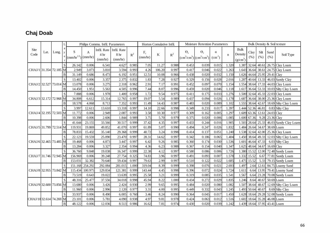
66
Chaj Doab
S 26.142 0.006 6.541 4.627 0.985 7.05 11.27 0.988 0.453 0.039 0.015 1.320 1.387 32.64 40.61 26.75 Clay Loam
M 2.949 3.073 3.810 3.594 0.993 4.26 106.20 0.997 0.417 0.046 0.022 1.263 1.643 36.64 38.61 24.75 Clay Loam
B 31.149 0.686 8.473 6.192 0.951 12.51 10.08 0.966 0.438 0.020 0.032 1.150 1.626 44.64 25.95 29.41 Clay
S 13.402 0.006 3.357 2.375 0.832 1.83 7.28 0.927 0.329 0.156 0.028 2.016 1.287 40.64 13.33 46.03 Sandy Clay
M 13.078 0.006 3.275 2.318 0.962 2.91 7.17 0.991 0.452 0.097 0.070 1.154 1.554 38.64 17.33 44.03 Clay Loam
B 14.450 1.951 5.563 4.505 0.996 7.44 8.07 0.996 0.459 0.020 0.046 1.118 1.617 36.64 53.33 10.03 Silty Clay Loam
S 7.888 0.006 1.978 1.400 0.958 1.72 9.54 0.975 0.411 0.175 0.033 1.276 1.500 32.64 45.33 22.03 Clay Loam
M 34.808 6.612 15.314 12.765 0.997 19.07 5.54 0.989 0.437 0.094 0.026 1.178 1.687 36.64 38.00 25.36 Clay Loam
B 18.578 4.068 8.713 7.352 0.993 11.49 14.43 0.987 0.483 0.020 0.089 1.102 1.555 38.64 42.67 18.69 Silty Clay Loam
S 3.997 12.611 13.610 13.318 0.997 14.10 22.66 0.998 0.349 0.233 0.017 1.397 1.444 52.36 46.81 0.83 Silty Clay
M 11.772 0.006 2.949 2.087 0.993 3.58 10.30 0.977 0.309 0.162 0.005 1.297 1.609 63.36 12.61 24.03 Clay
B 10.398 0.006 2.606 1.844 0.989 3.75 5.70 0.979 0.375 0.020 0.006 1.085 1.600 67.36 9.28 23.36 Clay
S 41.644 23.155 33.566 30.517 0.999 37.42 4.35 0.997 0.433 0.244 0.016 1.905 1.503 28.64 25.33 46.03 Sandy Clay Loam
M 119.931 19.869 49.852 41.070 0.997 61.89 5.07 0.990 0.494 0.247 0.026 1.832 1.484 26.64 34.67 38.69 Loam
B 78.833 15.432 35.140 29.368 0.999 40.72 3.24 0.998 0.414 0.137 0.051 1.240 1.538 32.64 42.00 25.36 Clay Loam
S 22.123 19.559 25.090 23.470 0.997 28.31 14.62 0.997 0.342 0.186 0.065 1.404 1.450 38.64 49.33 12.03 Silty Clay Loam
M 19.468 0.006 4.873 3.447 0.997 6.42 9.26 0.985 0.360 0.174 0.030 1.536 1.601 46.64 47.33 6.03 Silty Clay
B 13.284 0.006 3.327 2.354 0.994 4.36 6.23 0.988 0.367 0.154 0.040 1.347 1.625 48.64 34.67 16.69 Clay
S 36.760 9.848 19.038 16.347 0.999 22.38 4.12 0.997 0.580 0.086 0.006 1.726 1.380 15.52 12.00 72.48 Sandy Loam
M 156.969 0.006 39.248 27.754 0.325 74.83 3.96 0.997 0.491 0.093 0.007 1.578 1.332 15.52 6.67 77.81 Sandy Loam
B 153.031 32.382 70.640 59.434 0.997 79.63 2.99 0.997 0.510 0.122 0.022 1.685 1.475 15.52 5.33 79.15 Sandy Loam
S 151.168 254.292 292.084 281.015 1.000 319.04 8.39 0.999 0.398 0.076 0.021 2.693 1.497 2.64 12.61 84.75 Loamy Sand
M 115.434 100.975 129.834 121.381 0.999 143.44 4.45 0.998 0.396 0.072 0.024 1.724 1.611 6.64 13.95 79.41 Loamy Sand
B 73.519 0.643 19.022 13.639 0.995 25.58 3.21 0.999 0.319 0.085 0.035 1.541 1.567 6.64 23.28 70.08 Sandy Loam
S 48.316 25.477 37.556 34.018 0.998 45.94 8.22 1.000 0.434 0.272 0.029 1.835 1.246 8.64 40.67 50.69 Loam
M 13.680 0.006 3.426 2.424 0.930 2.99 9.65 0.995 0.484 0.020 0.080 1.082 1.507 38.64 48.67 12.69 Silty Clay Loam
B 11.960 0.006 2.996 2.120 0.977 3.31 4.00 0.995 0.449 0.332 0.043 1.245 1.493 50.64 40.67 8.69 Silty Clay
S 33.937 0.006 8.490 6.005 0.760 3.46 8.24 0.990 0.364 0.045 0.017 1.450 1.628 18.64 29.28 52.08 Sandy Loam
M 23.101 0.006 5.781 4.090 0.938 4.97 9.81 0.978 0.424 0.063 0.012 1.516 1.602 18.64 35.28 46.08 Loam
B 48.122 0.006 12.036 8.513 0.986 16.62 7.81 0.974 0.430 0.020 0.039 1.242 1.439 18.64 37.95 43.41 Loam
CHAJ/10 32.614 74.269
CHAJ/8 32.955 73.842
CHAJ/9 32.600 73.856
CHAJ/6 32.465 73.485
CHAJ/7 31.746 72.945
CHAJ/4 32.195 72.503
CHAJ/5 31.799 72.514
CHAJ/2 32.527 73.014
CHAJ/3 32.172 72.968
CHAJ/1 31.354 72.185
Clay
(%)
Silt
(%)
Sand
(%)R
2ϴs
(cm3/cm
3)
ϴr
(cm3/cm
3)
α
(cm-1
)n
Bulk
Density
(g/cm3)
A
(mm/hr)
Infil. Rate
4 hr
(mm/hr)
Infil. Rate
8 hr
(mm/hr)
R2
Fc
(mm/hr)K
Philips Commu. Infil. Parameters Horton Comulative Infil. Moisture Retention Parameters Bulk Density & Soil texture
S
(mm/hr1/2
)Soil Type
Site
CodeLat. Long.
L
a
y
e
r

67
Rachna Doab
S 26.933 0.006 6.739 4.767 0.994 8.91 4.61 0.986 0.503 0.070 0.008 1.559 1.343 31.76 55.23 13.01 Silty Clay Loam
M 19.910 0.006 4.983 3.526 0.984 6.13 4.39 0.998 0.460 0.020 0.025 1.268 1.494 35.76 24.56 39.68 Clay Loam
B 30.963 0.006 7.747 5.480 0.987 10.32 7.19 0.996 0.452 0.064 0.014 1.402 1.425 35.76 16.56 47.68 Sandy Clay
S 28.112 0.006 7.034 4.976 0.932 4.95 10.54 0.980 0.446 0.071 0.030 1.367 1.312 33.76 46.56 19.68 Silty Clay Loam
M 20.293 0.006 5.079 3.593 0.998 7.26 13.19 0.979 0.429 0.020 0.022 1.190 1.635 41.76 31.89 26.35 Clay
B 17.189 0.006 4.303 3.045 0.955 4.34 6.85 0.997 0.529 0.073 0.005 1.966 1.404 35.76 38.56 25.68 Clay Loam
S 18.694 0.852 5.526 4.157 0.997 7.65 6.50 0.992 0.455 0.020 0.006 1.286 1.454 33.76 60.56 5.68 Silty Clay Loam
M 6.165 1.024 2.565 2.114 0.967 3.45 12.29 0.964 0.447 0.100 0.005 1.662 1.411 41.76 44.56 13.68 Silty Clay
B 4.975 0.006 1.250 0.885 0.795 1.80 21.70 0.868 0.495 0.115 0.007 3.162 1.395 19.76 53.89 26.35 Silt Loam
S 29.840 1.564 9.024 6.839 0.998 11.69 4.09 0.997 0.478 0.030 0.019 1.258 1.428 37.76 45.89 16.35 Silty Clay Loam
M 27.777 0.006 6.950 4.916 0.992 8.78 19.88 0.988 0.470 0.020 0.012 1.326 1.590 35.76 37.23 27.01 Clay Loam
B 14.800 2.080 5.780 4.696 0.996 7.83 11.74 0.993 0.478 0.020 0.009 1.254 1.579 43.76 55.23 1.01 Silty Clay
S 16.683 0.006 4.177 2.955 0.928 3.49 7.47 0.955 0.420 0.020 0.010 1.214 1.541 36.64 55.12 8.24 Silty Clay Loam
M 15.676 4.367 8.287 7.139 0.976 10.38 16.91 0.995 0.404 0.020 0.010 1.233 1.657 38.64 29.79 31.57 Clay Loam
B 3.607 0.052 0.953 0.689 0.984 1.51 21.31 0.980 0.355 0.020 0.008 1.136 1.670 38.64 46.45 14.91 Silty Clay Loam
S 5.031 0.006 1.264 0.895 0.924 1.09 4.08 0.983 0.408 0.021 0.051 1.079 1.578 40.64 50.45 8.91 Silty Clay
M 15.363 11.240 15.081 13.956 0.996 17.07 7.42 0.992 0.472 0.118 0.015 1.308 1.467 48.64 34.45 16.91 Clay
B 5.340 13.208 14.543 14.152 0.999 15.14 6.83 0.998 0.505 0.097 0.017 1.216 1.451 56.64 28.45 14.91 Clay
S 12.281 0.006 3.076 2.177 0.944 3.08 7.15 0.921 0.363 0.163 0.040 1.355 1.495 29.36 33.28 37.36 Clay Loam
M 26.302 1.953 8.529 6.603 0.995 11.19 5.05 0.982 0.411 0.083 0.093 1.236 1.750 33.36 28.61 38.03 Clay Loam
B 40.531 2.671 12.804 9.836 0.997 17.16 5.40 0.984 0.468 0.105 0.029 1.492 1.756 29.36 23.28 47.36 Sandy Clay Loam
S 5.680 0.006 1.426 1.010 0.849 0.68 4.12 0.950 0.520 0.042 0.036 1.228 1.436 28.64 18.61 52.75 Sandy Clay Loam
M 17.326 0.006 4.338 3.069 0.971 3.08 2.58 0.995 0.602 0.185 0.009 1.739 1.500 32.64 21.95 45.41 Sandy Clay Loam
B 43.058 4.258 15.023 11.870 0.988 14.94 3.04 0.987 0.461 0.099 0.023 1.422 1.580 36.64 15.28 48.08 Sandy Clay
RCH/8 32.182 74.262
RCH/6 31.500 72.915
RCH/7 32.071 73.375
RCH/4 30.835 72.921
RCH/5 31.337 73.394
RCH/2 30.890 72.506
RCH/3 30.850 72.063
RCH/1 31.284 72.713
Clay
(%)
Silt
(%)
Sand
(%)R
2ϴs
(cm3/cm
3)
ϴr
(cm3/cm
3)
α
(cm-1
)n
Bulk
Density
(g/cm3)
A
(mm/hr)
Infil. Rate
4 hr
(mm/hr)
Infil. Rate
8 hr
(mm/hr)
R2
Fc
(mm/hr)K
Philips Commu. Infil. Parameters Horton Comulative Infil. Moisture Retention Parameters Bulk Density & Soil texture
S
(mm/hr1/2
)Soil Type
Site
CodeLat. Long.
L
a
y
e
r

68
Rachna Doab
S 69.923 0.901 18.382 13.262 0.998 26.06 5.45 0.996 0.534 0.119 0.025 1.375 1.380 22.64 14.61 62.75 Sandy Clay Loam
M 35.043 0.165 8.925 6.360 0.994 10.77 2.80 0.996 0.484 0.161 0.023 1.375 1.439 24.64 24.61 50.75 Sandy Clay Loam
B 31.881 0.006 7.976 5.642 0.994 9.98 3.98 0.996 0.504 0.102 0.019 1.478 1.490 24.64 30.61 44.75 Loam
S 41.912 0.006 10.484 7.415 0.999 15.15 6.73 0.989 0.479 0.056 0.041 1.202 1.345 20.64 19.28 60.08 Sandy Clay Loam
M 39.494 1.898 11.772 8.880 0.999 16.02 5.36 0.996 0.465 0.172 0.010 1.442 1.467 20.64 10.61 68.75 Sandy Clay Loam
B 35.242 2.601 11.411 8.831 0.998 14.66 4.41 0.995 0.495 0.073 0.016 1.402 1.456 18.64 6.61 74.75 Sandy Loam
S 27.615 4.332 11.235 9.213 0.997 13.72 4.15 0.998 0.513 0.051 0.027 1.238 1.428 38.64 41.28 20.08 Clay Loam
M 27.238 5.249 12.058 10.064 0.997 3.08 2.58 0.941 0.541 0.206 0.006 1.949 1.489 34.64 43.95 21.41 Clay Loam
B 22.955 3.296 9.035 7.354 0.998 14.94 3.04 0.990 0.516 0.096 0.012 1.502 1.521 30.64 41.95 27.41 Clay Loam
S 19.826 5.262 10.219 8.767 0.997 12.50 6.42 0.991 0.459 0.020 0.053 1.170 1.349 23.52 41.33 35.15 Loam
M 18.410 4.166 8.768 7.420 0.996 10.69 5.27 0.990 0.470 0.193 0.008 1.703 1.457 25.52 42.67 31.81 Loam
B 23.529 0.006 5.888 4.165 0.995 7.52 4.48 0.991 0.476 0.102 0.015 1.458 1.447 21.52 46.00 32.48 Loam
S 13.108 0.006 3.283 2.323 0.983 4.51 20.30 0.999 0.359 0.149 0.086 1.306 1.495 22.64 41.95 35.41 Loam
M 19.051 54.769 59.532 58.137 0.997 61.19 4.14 0.996 0.335 0.215 0.028 1.788 1.864 20.64 37.28 42.08 Loam
B 133.449 103.046 136.408 126.637 0.999 164.60 16.04 0.995 0.340 0.032 0.031 1.082 1.740 26.64 15.28 58.08 Sandy Clay Loam
S 16.688 0.540 4.712 3.490 0.999 6.55 5.52 0.995 0.351 0.140 0.018 1.774 1.751 25.20 29.33 45.47 Loam
M 10.160 0.006 2.546 1.802 0.998 3.57 10.22 0.980 0.322 0.127 0.030 1.519 1.849 25.20 27.33 47.47 Sandy Clay Loam
B 23.183 0.006 5.802 4.104 0.997 7.59 7.87 0.991 0.397 0.104 0.023 1.615 1.691 27.20 22.00 50.80 Sandy Clay Loam
S 15.704 0.006 3.932 2.782 0.999 5.58 6.56 0.994 0.396 0.070 0.012 1.409 1.755 37.20 39.33 23.47 Clay Loam
M 15.951 0.006 3.994 2.826 0.971 3.96 8.73 0.996 0.528 0.109 0.015 1.302 1.449 47.20 52.67 0.13 Silty Clay
B 6.867 0.006 1.723 1.220 0.990 1.81 12.28 0.988 0.366 0.254 0.019 1.561 1.693 43.20 42.00 14.80 Silty Clay
S 94.851 0.006 23.719 16.773 0.992 33.92 5.38 0.995 0.373 0.020 0.010 1.135 1.478 35.20 40.67 24.13 Clay Loam
M 0.001 47.737 47.737 47.737 0.975 47.74 144776.7 0.975 0.396 0.186 0.029 1.231 1.667 37.20 46.67 16.13 Silty ClaY Loam
B 2.088 0.006 0.528 0.375 0.319 0.11 64.79 0.461 0.404 0.020 0.020 1.085 1.619 53.20 38.67 8.13 Clay
RCH/16 32.263 75.246
RCH/14 32.126 73.995
RCH/15 32.170 74.690
RCH/12 31.318 73.854
RCH/13 32.536 74.631
RCH/10 31.755 74.298
RCH/11 31.744 73.403
RCH/9 31.744 73.832
Clay
(%)
Silt
(%)
Sand
(%)R
2ϴs
(cm3/cm
3)
ϴr
(cm3/cm
3)
α
(cm-1
)n
Bulk
Density
(g/cm3)
A
(mm/hr)
Infil. Rate
4 hr
(mm/hr)
Infil. Rate
8 hr
(mm/hr)
R2
Fc
(mm/hr)K
Philips Commu. Infil. Parameters Horton Comulative Infil. Moisture Retention Parameters Bulk Density & Soil texture
S
(mm/hr1/2
)Soil Type
Site
CodeLat. Long.
L
a
y
e
r

69
Bari Doab
S
(mm/hr1/2
)
A
(mm/hr)
Infil. Rate
4 hr
(mm/hr)
Infil. Rate
8 hr
(mm/hr)
R2
Fc
(mm/hr)K R
2ϴs
(cm3/cm
3)
ϴr
(cm3/cm
3)
α
(cm-1
)n
Bulk
Density
(g/cm3)
Clay
(%)
Silt
(%)
Sand
(%)Soil Type
S 22.595 0.006 5.655 4.000 0.995 7.71 8.46 0.978 0.490 0.112 0.008 1.509 1.245 36.64 51.28 12.08 Silty Clay Loam
M 8.674 0.006 2.175 1.539 0.875 1.72 11.28 0.962 0.440 0.020 0.015 1.113 1.599 70.64 17.95 11.41 Clay
B 9.231 0.006 2.314 1.638 0.868 1.43 14.66 0.985 0.427 0.020 0.010 1.136 1.677 64.64 15.95 19.41 Clay
S 20.232 0.006 5.064 3.583 0.991 6.99 7.88 0.981 0.450 0.020 0.019 1.204 1.421 40.64 55.95 3.41 Silty Clay
M 71.680 33.551 51.471 46.222 0.996 61.77 15.08 0.998 0.488 0.020 0.009 1.571 1.427 24.64 57.95 17.41 Silt Loam
B 32.918 20.958 29.188 26.777 0.997 33.78 14.50 0.999 0.490 0.043 0.009 2.102 1.363 20.64 43.95 35.41 Loam
S 9.170 1.000 3.293 2.621 0.995 4.24 4.86 0.992 0.491 0.134 0.026 1.345 1.201 41.20 53.89 4.91 Silty Clay
M 12.867 0.006 3.223 2.281 0.987 3.86 3.51 0.984 0.446 0.020 0.041 1.117 1.405 47.20 49.23 3.57 Silty Clay
B 20.195 0.006 5.055 3.576 0.987 4.95 4.48 0.985 0.457 0.020 0.021 1.098 1.379 45.20 49.23 5.57 Silty Clay
S 10.498 0.006 2.632 1.863 0.993 4.27 12.22 0.982 0.402 0.028 0.012 1.459 1.357 22.64 56.61 20.75 Silt Loam
M 17.574 0.006 4.400 3.113 0.996 3.78 8.86 0.983 0.347 0.020 0.011 1.462 1.420 20.64 54.61 24.75 Silt Loam
B 19.291 0.006 4.829 3.416 0.979 4.95 4.48 0.985 0.424 0.046 0.012 1.703 1.367 20.64 48.61 30.75 Loam
S 21.352 0.006 5.344 3.781 0.993 6.88 12.23 0.982 0.445 0.020 0.097 1.148 1.380 28.64 55.28 16.08 Silty Clay Loam
M 9.346 0.816 3.153 2.469 0.989 3.91 12.51 0.982 0.374 0.106 0.039 1.167 1.489 54.64 42.61 2.75 Silty Clay
B 14.414 0.868 4.472 3.416 0.997 0.82 5.79 0.931 0.428 0.085 0.026 1.343 1.490 34.64 59.28 6.08 Silty Clay Loam
S 21.974 0.006 5.500 3.890 0.996 6.88 12.23 0.982 0.395 0.118 0.013 1.722 1.375 24.64 47.33 28.03 Loam
M 12.278 0.006 3.076 2.177 0.990 3.91 12.51 0.989 0.455 0.067 0.021 1.540 1.320 22.64 54.67 22.69 Silt Loam
B 7.670 0.006 1.924 1.362 0.817 0.82 5.79 0.997 0.430 0.020 0.022 1.237 1.503 24.64 50.67 24.69 Silt Loam
S 13.488 0.006 3.378 2.390 0.997 4.27 12.22 0.982 0.462 0.084 0.020 1.320 1.301 38.64 59.28 2.08 Silty Clay Loam
M 13.305 0.006 3.332 2.358 0.985 3.78 8.86 0.983 0.483 0.020 0.021 1.245 1.343 30.64 67.61 1.75 Silty Clay Loam
B 19.291 0.006 4.829 3.416 0.979 4.95 4.48 0.985 0.446 0.098 0.066 1.164 1.389 62.64 36.77 0.59 Clay
S 6.127 1.129 2.661 2.212 0.997 3.33 5.87 0.997 0.447 0.090 0.028 1.386 1.254 28.64 62.61 8.75 Silty Clay Loam
M 38.767 0.006 9.698 6.859 0.981 13.53 6.73 0.955 0.416 0.102 0.018 1.483 1.433 32.64 59.28 8.08 Silty Clay Loam
B 25.742 6.357 12.793 10.908 0.991 12.73 1.96 0.994 0.423 0.060 0.106 1.216 1.410 30.64 55.28 14.08 Silty Clay Loam
S 19.284 0.006 4.827 3.415 0.981 5.32 6.85 0.992 0.422 0.071 0.010 1.522 1.415 34.08 61.33 4.59 Silty Clay Loam
M 18.176 0.006 4.550 3.219 0.980 5.03 6.36 0.975 0.457 0.153 0.012 1.302 1.495 44.08 53.33 2.59 Silty Clay
B 11.943 0.764 3.749 2.875 0.993 5.28 8.65 0.997 0.425 0.020 0.033 1.161 1.663 34.08 60.00 5.92 Silty Clay Loam
S 12.148 0.006 3.043 2.153 0.518 0.01 6.52 0.991 0.495 0.020 0.024 1.177 1.461 34.08 54.00 11.92 Silty Clay Loam
M 19.293 0.006 4.829 3.417 0.990 5.92 6.47 0.980 0.416 0.125 0.016 1.273 1.614 41.17 58.42 0.41 Silty Clay
B 14.533 1.962 5.595 4.531 0.997 7.31 6.56 0.988 0.464 0.070 0.037 1.151 1.589 40.08 39.33 20.59 Clay
LBD/10 31.275 74.288
LBD/8 30.938 73.811
LBD/9 30.884 74.073
LBD/6 30.449 73.859
LBD/7 31.045 73.536
LBD/4 30.402 72.202
LBD/5 30.905 73.378
LBD/2 30.419 71.697
LBD/3 30.447 73.389
LBD/1 30.487 72.110
Philips Commu. Infil. Parameters Horton Comulative Infil. Moisture Retention Parameters Bulk Density & Soil texture
Site
CodeLat. Long.
L
a
y
e
r

70
Bari Doab
S
(mm/hr1/2
)
A
(mm/hr)
Infil. Rate
4 hr
(mm/hr)
Infil. Rate
8 hr
(mm/hr)
R2
Fc
(mm/hr)K R
2ϴs
(cm3/cm
3)
ϴr
(cm3/cm
3)
α
(cm-1
)n
Bulk
Density
(g/cm3)
Clay
(%)
Silt
(%)
Sand
(%)Soil Type
S 15.788 0.006 3.953 2.797 0.957 3.45 4.12 0.993 0.405 0.020 0.029 1.155 1.401 21.20 64.11 14.69 Silt Loam
M 11.414 0.006 2.860 2.024 0.976 2.88 8.97 0.990 0.437 0.052 0.018 1.234 1.411 23.20 58.77 18.03 Silt Loam
B 4.629 0.006 1.163 0.824 0.993 1.78 11.69 0.975 0.406 0.020 0.057 1.095 1.539 33.20 58.11 8.69 Silty Clay Loam
S 25.069 0.075 6.342 4.507 0.996 196.79 29.79 0.999 0.446 0.071 0.009 1.248 1.517 28.64 52.67 18.69 Silty Clay Loam
M 13.724 2.434 5.865 4.861 0.998 145.67 17.04 0.999 0.454 0.020 0.010 1.509 1.310 22.64 36.67 40.69 Loam
B 22.210 0.006 5.558 3.932 0.994 70.10 21.31 0.999 0.476 0.043 0.020 1.326 1.310 24.64 36.67 38.69 Loam
S 11.973 1.785 4.778 3.901 0.994 6.56 15.01 0.989 0.507 0.124 0.008 1.924 1.395 24.48 60.61 14.91 Silt Loam
M 28.298 0.006 7.080 5.008 0.956 6.57 7.85 0.968 0.561 0.089 0.012 1.512 1.448 36.48 57.28 6.24 Silty Clay Loam
B 23.626 0.006 5.912 4.182 0.998 8.29 9.74 0.976 0.473 0.064 0.023 1.361 1.456 34.48 52.61 12.91 Silty Clay Loam
S 457.695 0.000 50.115 8.869 0.837 7.05 11.27 0.988 0.435 0.020 0.012 1.313 1.501 31.20 45.23 23.57 Clay Loam
M 203.248 0.000 13.506 2.358 0.802 3.78 8.86 0.983 0.418 0.086 0.011 1.420 1.501 27.20 57.89 14.91 Silty Clay Loam
B 346.645 5.807 8.469 11.870 0.676 17.47 3.36 0.986 0.430 0.033 0.010 1.310 1.507 21.20 71.23 7.57 Silt Loam
S 37.184 0.429 8.856 6.388 0.993 11.62 3.26 0.994 0.420 0.020 0.010 1.214 1.385 25.44 48.67 25.89 Loam
M 18.127 0.006 4.237 2.998 0.980 4.90 5.06 0.989 0.404 0.020 0.010 1.233 1.572 23.44 45.33 31.23 Loam
B 12.623 0.697 3.494 2.632 0.998 5.23 9.85 0.982 0.355 0.020 0.008 1.136 1.465 19.44 47.33 33.23 Loam
S 21.109 0.142 5.419 3.874 0.988 9.18 1066.81 0.963 0.431 0.154 0.011 1.549 1.477 21.44 39.33 39.23 Loam
M 20.288 13.952 19.024 17.538 0.997 22.43 1008.91 0.994 0.467 0.020 0.023 1.323 1.464 31.44 60.67 7.89 Silty Clay Loam
B 13.107 0.006 3.283 2.323 0.986 4.99 1282.32 0.920 0.452 0.020 0.004 1.226 1.437 9.44 52.00 38.56 Silt Loam
S 16.158 0.024 4.064 2.881 0.996 6.94 1411.88 0.947 0.382 0.136 0.004 1.667 1.463 23.44 56.00 20.56 Silt Loam
M 20.518 0.006 5.136 3.633 0.985 7.55 826.12 0.896 0.471 0.073 0.010 1.519 1.424 21.44 57.33 21.23 Silt Loam
B 23.516 0.006 5.885 4.163 0.954 9.07 752.91 0.840 0.491 0.103 0.004 2.032 1.380 21.44 73.33 5.23 Silt Loam
S 24.767 0.006 6.198 4.384 0.981 9.96 830.73 0.890 0.455 0.130 0.007 1.762 1.490 16.16 61.33 22.51 Silt Loam
M 12.059 100.863 103.878 102.995 0.999 105.74 1558.78 0.999 0.380 0.064 0.008 1.871 1.282 6.16 60.67 33.17 Silt Loam
B 0.001 197.170 197.170 197.170 0.998 197.17 63615.51 0.998 0.404 0.030 0.005 2.567 1.135 4.16 64.67 31.17 Silt Loam
S 14.224 0.006 3.562 2.520 0.984 5.68 1414.73 0.908 0.462 0.137 0.007 1.706 1.446 21.44 58.67 19.89 Silt Loam
M 13.238 15.381 18.690 17.721 0.996 21.22 1760.60 0.989 0.532 0.085 0.006 2.060 1.368 9.44 77.33 13.23 Silt Loam
B 37.440 0.006 9.366 6.625 0.873 10.75 338.12 0.736 0.623 0.035 0.020 1.879 1.350 5.44 65.33 29.23 Silt Loam
S 15.299 0.006 3.831 2.710 0.990 284.80 4.53 0.993 0.434 0.036 0.011 1.273 1.419 23.44 54.00 22.56 Silt Loam
M 7.246 1.024 2.835 2.305 0.985 284.80 4.53 0.955 0.428 0.095 0.010 1.338 1.514 29.44 50.67 19.89 Silty Clay Loam
B 6.562 3.577 5.218 4.737 0.999 6.44 2144.17 0.984 0.393 0.192 0.012 1.257 1.534 27.44 60.67 11.89 Silty Clay Loam
LBD/20 29.567 71.836
LBD/18 29.677 71.197
LBD/19 29.619 71.554
LBD/16 30.032 72.636
LBD/17 30.092 71.619
LBD/14 30.544 72.694
LBD/15 30.027 72.268
LBD/12 30.067 72.945
LBD/13 30.692 73.168
LBD/11 31.593 74.547
Philips Commu. Infil. Parameters Horton Comulative Infil. Moisture Retention Parameters Bulk Density & Soil texture
Site
CodeLat. Long.
L
a
y
e
r

71