No. 0514

Social Protection Discussion Paper Series

How Does Working as a Child Affect Wage, Income and Poverty as an

Adult?

Nadeem Ilahi Peter F. Orazem

Guilherme Sedlacek

May 2005

Social Protection Unit

Human Development Network

The World Bank

Social Protection Discussion Papers are not formal publications of the World Bank. They present preliminary and unpolished results of analysis that are circulated to encourage discussion and comment; citation and the use of such a paper should take account of its provisional character. The findings, interpretations, and conclusions expressed in this paper are entirely those of the author(s) and should not be attributed in any manner to the World Bank, to its affiliated organizations or to members of its Board of Executive Directors or the countries they represent.

For free copies of this paper, please contact the Social Protection Advisory Service, The World Bank, 1818 H Street, N.W., Washington, D.C. 20433 USA. Telephone: (202) 458-5267, Fax: (202) 614-0471, E-mail: socialprotection@worldbank.org. Or visit the Social Protection website at http://www.worldbank.org/sp.

How Does Working as a Child affect Wage, Income and Poverty as an Adult?∗

Nadeem Ilahi

Peter F. Orazem

Guilherme Sedlacek

May 2005

∗ Excerpts obtained from the IADB/WB joint book on child labor in LAC

1

How Does Working as a Child Affect Wages, Income and

Poverty as an Adult?

Nadeem Ilahi Peter F. Orazem

Guilherme Sedlacek

Parents have their children specialize in schooling rather than go to work in part because

they expect that children will earn enough as adults to repay the lost earnings as a child.

However, children from poor households may not have the luxury of waiting to grow up before

entering the labor market. Sending their children to work may be the only option poor parents

have to sufficiently raise income to meet current consumption needs, so poor parents forego the

increased future income opportunity to meet basic necessities. One argument for government

efforts to limit child labor is that poor parents may under-invest in their children's education

relative to the social optimum. Those parents' decisions may not take into account societal

returns associated with improved education such as poverty reduction, slower population growth,

improved health, reduced crime, and a lower dependence on government transfer programs.

The rationale for government intervention assumes that children who do not work will

earn more as adults, and that these future returns are sufficiently high to justify the current loss of

income from reduced child labor. However, there is very little empirical research on the impact

of child labor on the child's earnings potential as an adult. Empirical estimation is necessary

because theory yields ambiguous predictions about the impact of early labor market entry on

lifetime earnings. Child labor need not lower lifetime earnings, and could even increase lifetime

earnings for some children.

One way child labor can alter adult earnings is by changing the number of years of

schooling children attain. Past studies have shown that a child’s years of schooling may be

2

increased or decreased when the child works. Psacharopoulos (1997) found evidence that child

labor lowered grade attainment, while Akabayashi and Psacharopoulos (1999) found that child

labor lowered measured school achievement per year. Other studies have found the opposite

results, however. Because many working children also are in school, some analysts have

suggested that child labor and schooling are not mutually exclusive (Ravallion and Wodon 2000)

and may even be complementary activities (Patrinos and Psacharopoulos 1997). One reason is

that child labor may raise household income sufficiently to allow the household to afford to send

at least some of their children to school, whether it is the working children or their siblings.

Without income derived from working children, these households may not be able to send any

children to school.

It is even possible that child labor can raise lifetime earnings of children as adults.

Standard theory of earnings initiated by Mincer (1974) argues that work experience raises wages,

presumably because human capital is generated through learning by doing. It is possible that

returns to a year of work experience dominate the returns to a year of schooling, particularly in

developing countries where schools available to poor households often are of poor quality. It also

is possible that by increasing current household income, child labor allows the parents to build an

endowment of physical assets that can be transferred to the child at maturity. These physical

assets may have a greater return in credit-constrained developing countries than do the foregone

human capital assets.1

This study measures the impact of child labor on adult wages and poverty incidence

through each of these potential avenues. Using a unique data set on adult earnings in Brazil, child

labor is allowed to affect adult earnings through its impacts on work experience, years of

1 Parsons and Goldin (1989) found that in U.S. households in 1890, child labor income primarily went toward current household consumption and little if any physical assets were transferred to working children when they reached adulthood.

3

schooling, and human capital attained per year of schooling. Adding up these positive and

negative effects, the empirical findings demonstrate that early entry to the workforce reduces

lifetime earnings by 13% to 20%. Child labor also raises the probability of being poor later in life

by 13% to 31%.

These findings have important policy implications. Reducing child labor can significantly

improve children's adult wages, income, and poverty status, so governments can trade off current

costs of child labor eradication programs against future lower costs of poverty programs and/or

increased tax returns. Policies that keep working children in school also are supported because

the positive effect of increased educational attainment on adult income is larger than the negative

effect of child labor on earnings.

Trends and Tradeoffs Between Child Labor and Education in Brazil

As shown by Duryea et al. (Chapter 4), the incidence of child labor in Brazil has

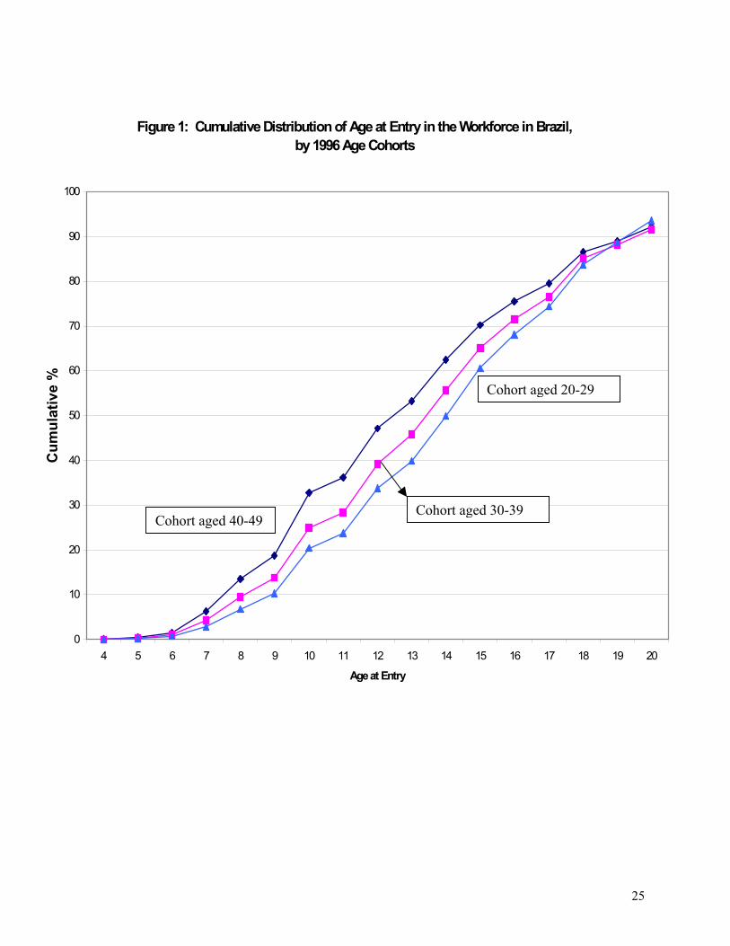
decreased over time. The cumulative distribution of the age of workforce entry by birth cohort is

presented in figure 1. The median age at entry was 12.5 for the cohort aged 40 to 49 in 1996. It

increased 1.5 years to age 14 for the cohort aged 20 to 29. Much of the change in average cohort

age is due to the decreasing frequency of very early entry into the labor force. One-third of the

cohort aged 40 to 49 had entered the labor force by age 10, but the incidence had fallen to 20%

for the cohort aged 20 to 29.

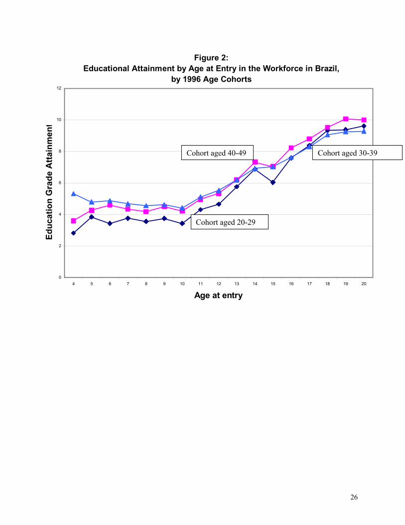
The relationship between age of labor market entry and years of education by birth cohort

is illustrated in figure 2. The relationship is quite stable across birth cohorts. Overall, as age of

labor market entry increases, years of education completed also increase. However, there is no

gain in average schooling by delaying labor market entry from age 4 to age 10. Over that range,

average schooling remains constant at four years. One interpretation of figure 2 is that the

4

increasing educational attainment in Brazil is due not to increased educational attainment of

working children, but to delayed age of labor market entry for more recent birth cohorts.

There is a strong circumstantial case that early entry into the labor market has adverse

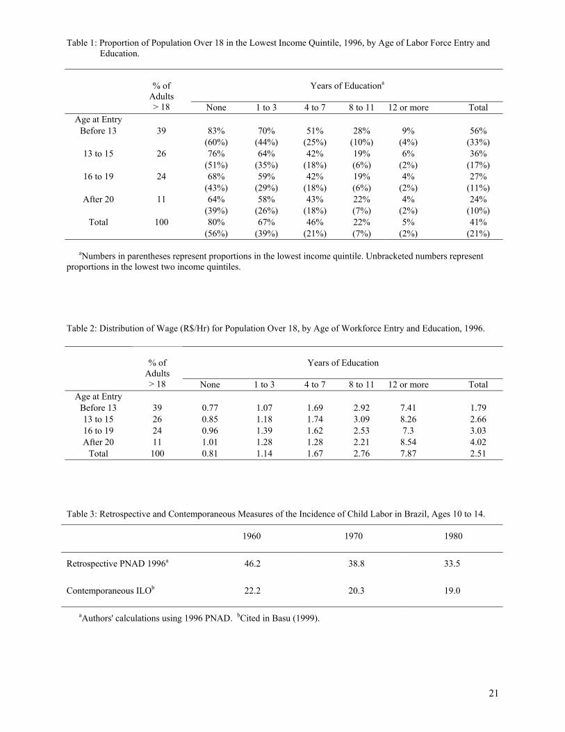
consequences for adult income. Table 1 reports the probability of beimng in the lowest income

quintile as an adult by years of education and age of labor market entry. The lowest income

quintile in Brazil can be viewed as being extremelyu poor by nternatiopnal standards. The

probability of being extremely poor declines as age of labor market entry and years of education

increase. Child labor appears to be particularly damaging for the 39% of adults who began

working before age 13. Of those, 56% are in the lowest two income quintiles, and one-third are

in the lowest income quintile. However, increasing years of education mitigates the impact of

early labor market entry.

Table 2 shows similar adverse impacts of early labor market entry on wages as an adult.

Those who entered before age 13 earned 49% less than those who entered between the ages of 13

and 15. Again, education appears to mitigate the effect. For those with at least four to seven

years of education, generally considered sufficient to attain literacy, the adverse effects of early

labor market entry become less clear.

These findings suggest that if a working child remains in school, adult earnings may not

suffer. That fact supports the argument that policies restricting child labor could do more harm

than good. In Brazilian households that have child workers, child labor represents 17% of urban

household income and 22% of rural household income. Given the strong positive effect of

household income on child schooling, it is plausible that child labor could self-correct its adverse

consequences on adult earnings by inducing additional years of schooling. Econometric

estimation is necessary to assess whether these positive aspects of child labor outweigh the

apparent negatives for lifetime earnings.

5

Theory

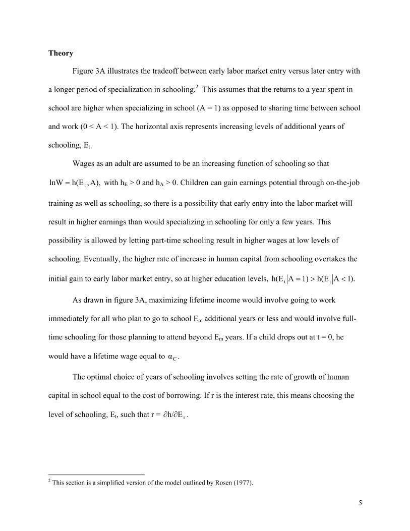
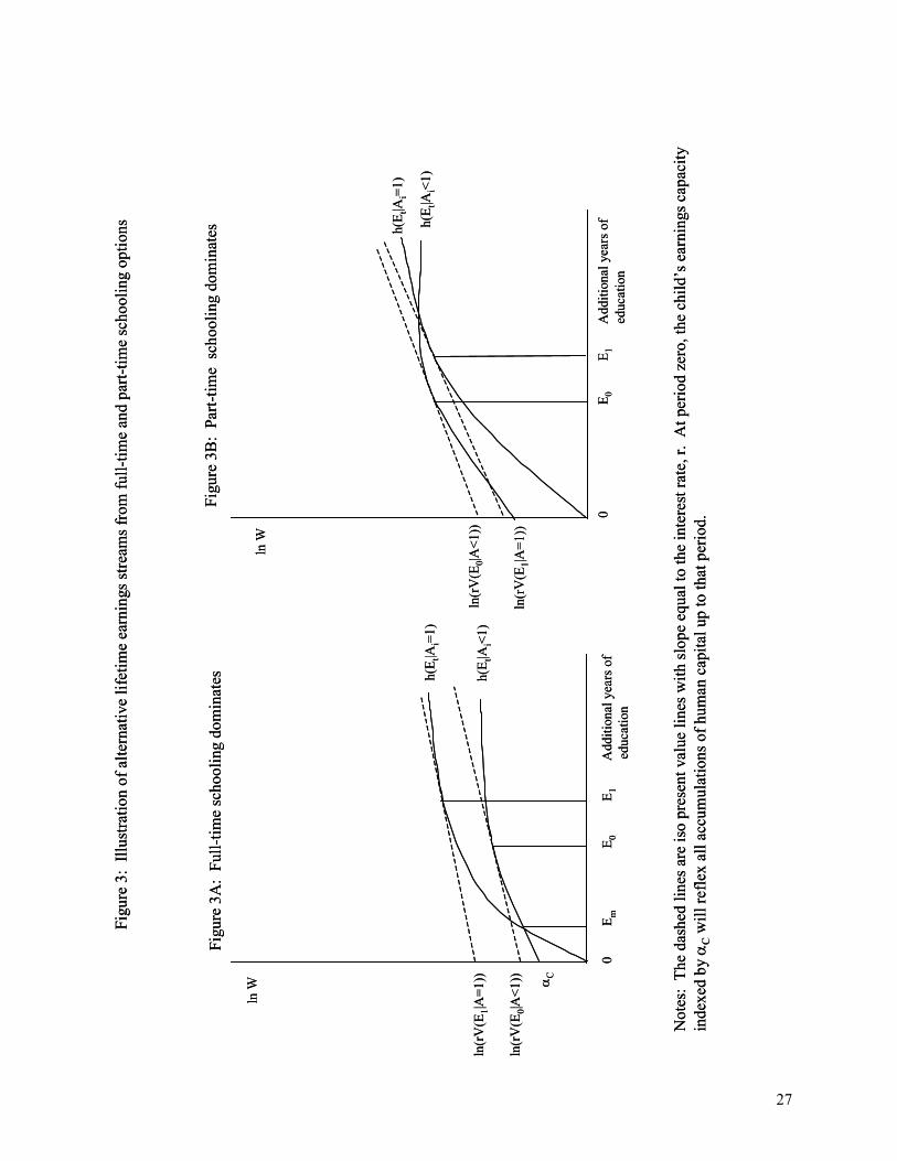
Figure 3A illustrates the tradeoff between early labor market entry versus later entry with

a longer period of specialization in schooling.2 This assumes that the returns to a year spent in

school are higher when specializing in school (A = 1) as opposed to sharing time between school

and work (0 < A < 1). The horizontal axis represents increasing levels of additional years of

schooling, Et.

Wages as an adult are assumed to be an increasing function of schooling so that

A),,h(ElnW t= with hE > 0 and hA > 0. Children can gain earnings potential through on-the-job

training as well as schooling, so there is a possibility that early entry into the labor market will

result in higher earnings than would specializing in schooling for only a few years. This

possibility is allowed by letting part-time schooling result in higher wages at low levels of

schooling. Eventually, the higher rate of increase in human capital from schooling overtakes the

initial gain to early labor market entry, so at higher education levels, ).1Ah(E1)Ah(E tt <>=

As drawn in figure 3A, maximizing lifetime income would involve going to work

immediately for all who plan to go to school Em additional years or less and would involve full-

time schooling for those planning to attend beyond Em years. If a child drops out at t = 0, he

would have a lifetime wage equal to Cα .

The optimal choice of years of schooling involves setting the rate of growth of human

capital in school equal to the cost of borrowing. If r is the interest rate, this means choosing the

level of schooling, Et, such that r = tEh/∂∂ .

2 This section is a simplified version of the model outlined by Rosen (1977).

6

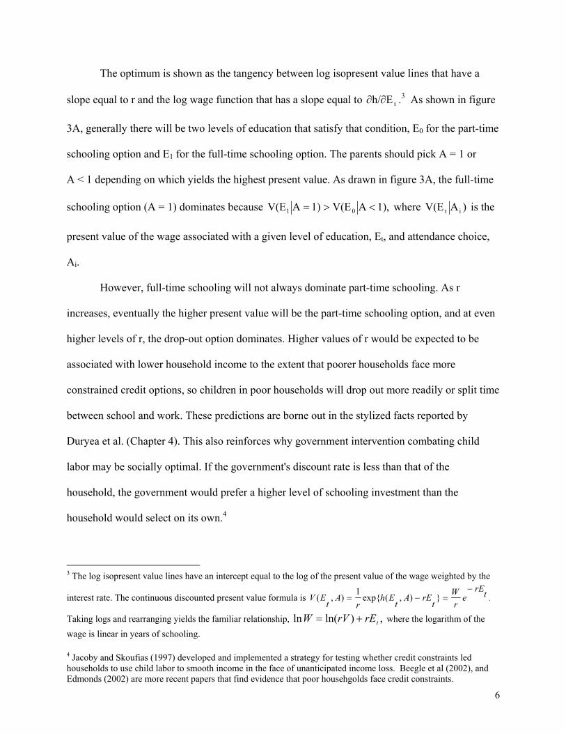
The optimum is shown as the tangency between log isopresent value lines that have a

slope equal to r and the log wage function that has a slope equal to tEh/∂∂ .3 As shown in figure

3A, generally there will be two levels of education that satisfy that condition, E0 for the part-time

schooling option and E1 for the full-time schooling option. The parents should pick A = 1 or

A < 1 depending on which yields the highest present value. As drawn in figure 3A, the full-time

schooling option (A = 1) dominates because ,1)AV(E1)AV(E 01 <>= where )AV(E it is the

present value of the wage associated with a given level of education, Et, and attendance choice,

Ai.

However, full-time schooling will not always dominate part-time schooling. As r

increases, eventually the higher present value will be the part-time schooling option, and at even

higher levels of r, the drop-out option dominates. Higher values of r would be expected to be

associated with lower household income to the extent that poorer households face more

constrained credit options, so children in poor households will drop out more readily or split time

between school and work. These predictions are borne out in the stylized facts reported by

Duryea et al. (Chapter 4). This also reinforces why government intervention combating child

labor may be socially optimal. If the government's discount rate is less than that of the

household, the government would prefer a higher level of schooling investment than the

household would select on its own.4

3 The log isopresent value lines have an intercept equal to the log of the present value of the wage weighted by the

interest rate. The continuous discounted present value formula is .}),(exp{1

),( trEe

rW

trEA

tEh

rA

tEV

−=−=

Taking logs and rearranging yields the familiar relationship, ,)ln(ln trErVW += where the logarithm of the wage is linear in years of schooling. 4 Jacoby and Skoufias (1997) developed and implemented a strategy for testing whether credit constraints led households to use child labor to smooth income in the face of unanticipated income loss. Beegle et al (2002), and Edmonds (2002) are more recent papers that find evidence that poor househgolds face credit constraints.

7

Part-time schooling and drop-out also are more likely to dominate when schools are poor,

so that earnings growth from schooling is slower. Figure 3B illustrates this point. Holding r at the

same level as in 3A, a flatter profile for h(Et|A = 1) now results in the part-time schooling option

having the higher present value of earnings.

This model demonstrates that early entry into the labor market could raise lifetime

wealth, particularly for children facing poor schools and high discount rates. Whether child labor

does in fact raise or lower measured adult wealth indicators requires empirical investigation.

Data

The analysis is based on the 1996 round of the national sample survey of households,

Pesquisa Nacional por Amostra de Domicílios (PNAD). PNAD, conducted annually by the

Brazilian government, is a nationally representative stratified random sample of the Brazilian

population designed to monitor the socioeconomic characteristics of the population including

education, labor, residency, and earnings. The 1996 survey is particularly suited to the needs of

this study in that it includes a retrospective question on age of labor market entry and

information about the parents of a subset of the adult respondents.

This study's empirical estimates of the impact of child labor on lifetime earnings rely on

the ability of respondents to recall whether they worked when they were young. In theory, recall

bias should be less severe for repeated activities such as work, but it is useful to compare the

recall data to contemporaneously collected data on the incidence of child labor. The implied

child labor force participation rates based on recall data are larger than the official rates reported

by the International Labor Organization (ILO), as shown in table 3.

8

Two reasons indicate why the retrospective data show a higher incidence of child labor

than would contemporaneously collected surveys. The first is that children are likely to enter and

exit the labor market, as demonstrated by Duryea et al. (Chapter 4). Consequently, those who

first entered the labor market at an early age may not have remained in the labor force

continuously thereafter. The second is that the retrospective data capture informal and part-time

work that may not be captured in contemporaneous survey data. In contrast, the ILO data refer

only to full-time work. In his survey of child labor literature, Basu (1999) reported that when

ILO estimates were adjusted to include part-time work, the incidence of child labor more than

doubled. In fact, the incidence of child labor implied by the retrospective data reported in table 3

is nearly twice that of the ILO estimates. Thus, the retrospective data track the

contemporaneously collected data quite well.

Estimation Strategy

There is a long tradition of examining returns to school by using earnings functions.

Following Welch (1966), analysis of returns to education was extended to incorporate returns to

school quality. Card and Krueger (1992) used a similar strategy to analyze the effects of school

and teacher attributes on lifetime earnings. Child labor can be incorporated into the earnings

function framework in the same manner as school quality. To begin, approximate the true

structural relationship between education, E, and child labor, C, as:

ii CCE β=)( (1)

where the parameter β captures the effects of early labor force entry on lifetime educational

attainment. The coefficient β can be positive or negative.

Now consider the complete relationship between earnings (and poverty) and child labor.

Consider the log earnings function:

9

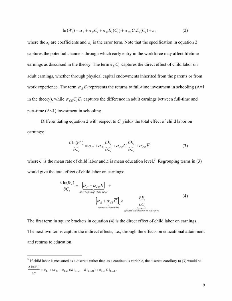
iiiiCEiiEiCi CECCECW εαααα ++++= )()()(ln 0 (2)

where the iα are coefficients and iε is the error term. Note that the specification in equation 2

captures the potential channels through which early entry in the workforce may affect lifetime

earnings as discussed in the theory. The term iCCα captures the direct effect of child labor on

adult earnings, whether through physical capital endowments inherited from the parents or from

work experience. The term iE Eα represents the returns to full-time investment in schooling (A=1

in the theory), while iiCE ECα captures the difference in adult earnings between full-time and

part-time (A<1) investment in schooling.

Differentiating equation 2 with respect to Ci yields the total effect of child labor on

earnings:

ECE

CCE

CW

CEi

iCE

i

iEC

i

i αααα +∂∂

+∂∂

+=∂

∂ )ln( (3)

where C is the mean rate of child labor and E is mean education level.5 Regrouping terms in (3)

would give the total effect of child labor on earnings:

[ ]

[ ]{

educationonlaborchildofeffecti

i

educationtoreturns

CEE

laborchildofeffectdirect

CECi

i

CE

C

ECW

∂∂

×+

++=∂

∂

4434421

43421

αα

αα)ln(

(4)

The first term in square brackets in equation (4) is the direct effect of child labor on earnings.

The next two terms capture the indirect effects, i.e., through the effects on educational attainment

and returns to education.

5 If child labor is measured as a discrete rather than as a continuous variable, the discrete corollary to (3) would be

1|)0|1|)(()ln(

=+=−=++=∆

∆CECECECECEEC

C

iWαααα .

10

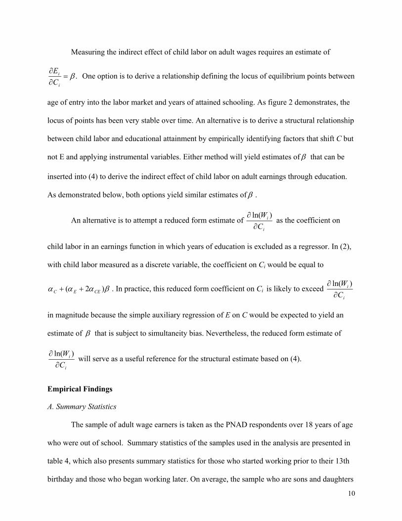
Measuring the indirect effect of child labor on adult wages requires an estimate of

.β=∂∂

i

i

CE

One option is to derive a relationship defining the locus of equilibrium points between

age of entry into the labor market and years of attained schooling. As figure 2 demonstrates, the

locus of points has been very stable over time. An alternative is to derive a structural relationship

between child labor and educational attainment by empirically identifying factors that shift C but

not E and applying instrumental variables. Either method will yield estimates of β that can be

inserted into (4) to derive the indirect effect of child labor on adult earnings through education.

As demonstrated below, both options yield similar estimates of β .

An alternative is to attempt a reduced form estimate of i

i

CW

∂∂ )ln(

as the coefficient on

child labor in an earnings function in which years of education is excluded as a regressor. In (2),

with child labor measured as a discrete variable, the coefficient on Ci would be equal to

βααα )2( CEEC ++ . In practice, this reduced form coefficient on Ci is likely to exceed i

i

CW

∂∂ )ln(

in magnitude because the simple auxiliary regression of E on C would be expected to yield an

estimate of β that is subject to simultaneity bias. Nevertheless, the reduced form estimate of

i

i

CW

∂∂ )ln(

will serve as a useful reference for the structural estimate based on (4).

Empirical Findings

A. Summary Statistics

The sample of adult wage earners is taken as the PNAD respondents over 18 years of age

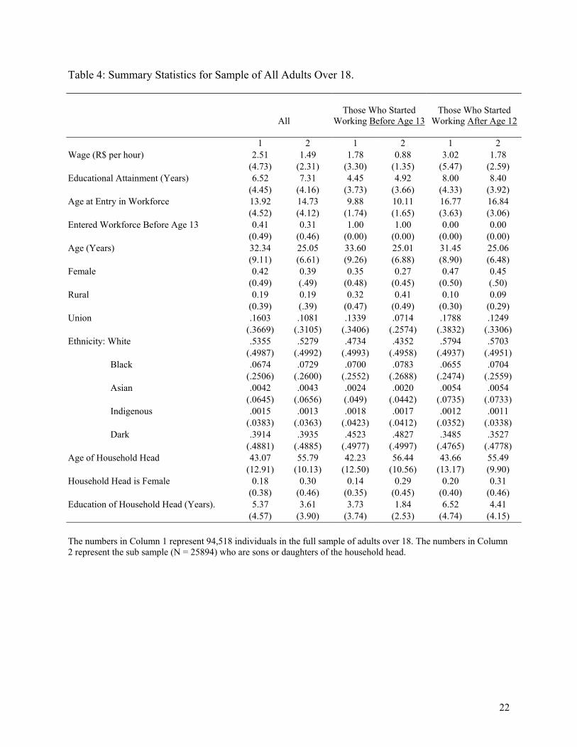
who were out of school. Summary statistics of the samples used in the analysis are presented in

table 4, which also presents summary statistics for those who started working prior to their 13th

birthday and those who began working later. On average, the sample who are sons and daughters

11

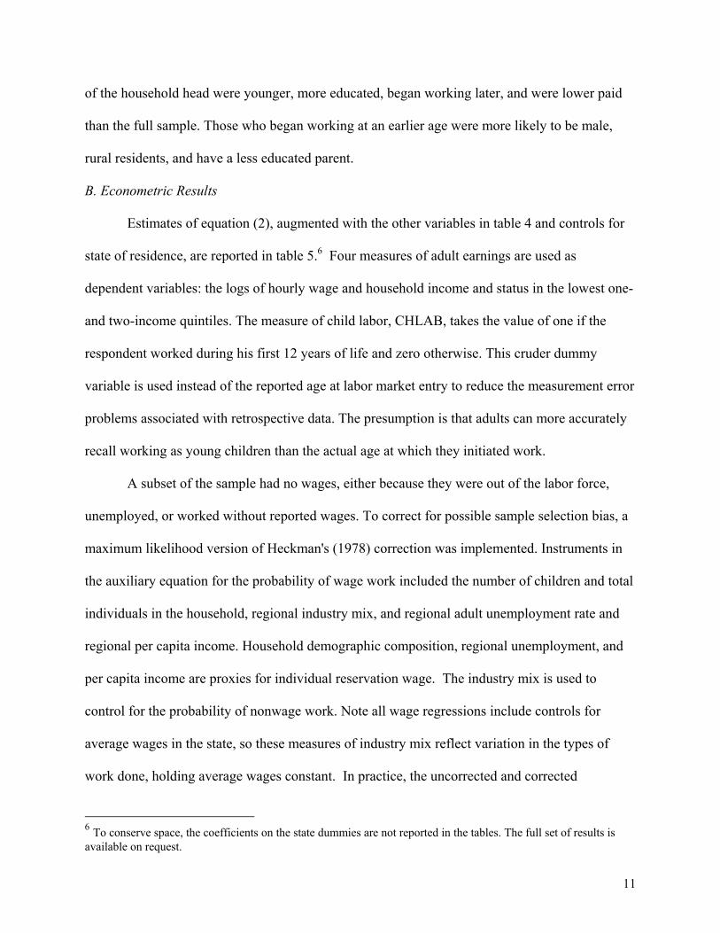
of the household head were younger, more educated, began working later, and were lower paid

than the full sample. Those who began working at an earlier age were more likely to be male,

rural residents, and have a less educated parent.

B. Econometric Results

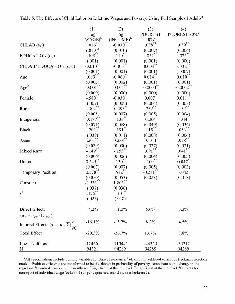
Estimates of equation (2), augmented with the other variables in table 4 and controls for

state of residence, are reported in table 5.6 Four measures of adult earnings are used as

dependent variables: the logs of hourly wage and household income and status in the lowest one-

and two-income quintiles. The measure of child labor, CHLAB, takes the value of one if the

respondent worked during his first 12 years of life and zero otherwise. This cruder dummy

variable is used instead of the reported age at labor market entry to reduce the measurement error

problems associated with retrospective data. The presumption is that adults can more accurately

recall working as young children than the actual age at which they initiated work.

A subset of the sample had no wages, either because they were out of the labor force,

unemployed, or worked without reported wages. To correct for possible sample selection bias, a

maximum likelihood version of Heckman's (1978) correction was implemented. Instruments in

the auxiliary equation for the probability of wage work included the number of children and total

individuals in the household, regional industry mix, and regional adult unemployment rate and

regional per capita income. Household demographic composition, regional unemployment, and

per capita income are proxies for individual reservation wage. The industry mix is used to

control for the probability of nonwage work. Note all wage regressions include controls for

average wages in the state, so these measures of industry mix reflect variation in the types of

work done, holding average wages constant. In practice, the uncorrected and corrected

6 To conserve space, the coefficients on the state dummies are not reported in the tables. The full set of results is available on request.

12

parameter estimates were virtually identical, so issues of selection appear not to have been that

critical. Only the selection-corrected estimates are reported to conserve space.

The log wage equations mimic standard results. Wages have a concave pattern over the

life cycle. The implied returns to schooling of 10.8% per year were consistent with those

reported by Lam and Schoeni (1993) for Brazil when controlling for family background

variables. Wages were higher for urban, male, and unionized workers, and were lower for

minority groups except Asians. Workers in jobs that were not permanent also were paid a

premium.

The parameters of primary interest are .and,, CEEC ααα Interestingly, ,0>Cα

suggesting that at zero years of education, child labor leads to higher lifetime earnings. This is

consistent with the presumption that child labor can increase human capital through on-the-job

training. However, child labor also makes education less efficient at producing human capital, so

.0<CEα Before proceeding to the numerical estimate of child labor on adult earnings, the

impact of child labor on years of schooling attained must be derived, CE∂∂ .

C. The Effect of Child Labor on Years of Education

As discussed in the introduction, past studies have disagreed about whether child labor

increases or decreases years of education. Such estimates are needed to derive the indirect impact

of child labor on earnings through the implied impact on human capital. The equilibrium locus of

points in figure 2 suggests that for each year the child remains out of the labor market past the

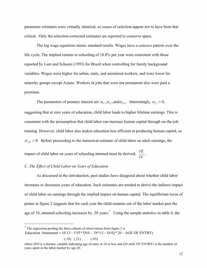
age of 10, attained schooling increases by .58 years.7 Using the sample statistics in table 4, the

7 The regression pooling the three cohorts of observations from figure 2 is

(.03)(.21)(.18)ENTRY)OFAGE20*D10)(1*.58D10*5.9510.13AttainmentEducation −−−−=

where D10 is a dummy variable indicating age of entry at 10 or less and (20-AGE OF ENTRY) is the number of years spent in the labor market by age 20.

13

average age of labor market entry for those who did not work in their first 12 years was 16.77

years, implying 4.77 years of additional specialization in schooling. The implied increase in

years of schooling for those who began working after age 12 is .58·(4.77) = 2.8 years. The

corresponding estimate in Psacharopoulos' (1997) study of Bolivian and Venezuelan working

children is two years of reduced educational attainment.

These are not structural estimates, however. To the extent that years of education and

child labor are simultaneously determined, these estimates based on market equilibrium

outcomes should overstate the true impact of child labor on years of completed schooling. To

address this problem, the study used a subset of the PNAD sample of adults who were still living

with their parents. Because the PNAD collected information on all household members, there is

information on household demographics including the number of siblings as well as education

and gender of the household head. That subset permits prediction of the incidence of child labor

using household attributes and local labor market conditions as instruments. The predicted

probability of child labor was used in a second-stage estimate explaining variation in completed

years of schooling.

In particular, the structural impact of child labor on schooling was estimated using a

probit equation of the form

CeRHXC +++= 321 γγγ , (5)

where C is a dichotomous variable indicating whether the adult worked in the first 12 years of

life, H is a vector of household attributes believed to affect the child's reservation wage, R is a

vector of local industry shares that should affect the market opportunities for child labor in the

14

region without altering returns to schooling8, and X includes demographic and economic factors

believed to affect both child labor and education choices. The predicted probability of working

as a child was then inserted into a second-stage regression explaining completed years of

education, E:

EeXCE ++= δβ ˆ , (6)

The sample on which the estimation of equations (5) and (6) is based is not random. Adults who

are living with their parents are likely to be atypically low-skilled and unsuccessful in the labor

market. For that reason, the estimate for (6) uses the maximum likelihood variant of the

Heckman sample selection model to control for possible self-selection in the sample of adults

living with their parents.

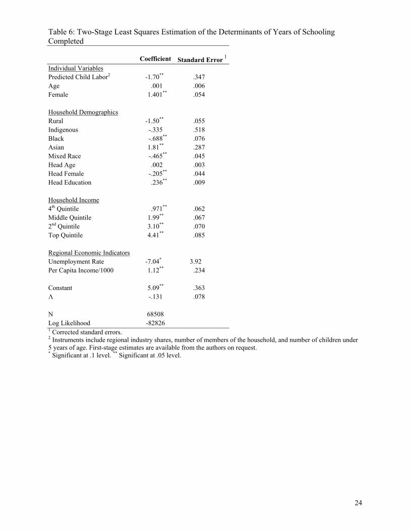
The results from the second-stage estimation are reported in table 6. Standard errors of

the coefficient are corrected for the two-step procedure using a bootstrap procedure. Other things

equal, children in urban areas finish 1.5 more years of school on average than do their rural

counterparts. Children in regions with low unemployment and high per capita income attend

school longer, so stronger labor demand helps keep children in school, presumably because the

parents remain employed. Girls complete 1.4 more years on average than do boys. Child

schooling also is positively related to the household head's education and the household's income

status.

Turning to the primary coefficient of interest, working in the first 12 years of life lowers

completed years of schooling by 1.7 years relative to otherwise identical individuals from

observationally identical households. The magnitude appears to be reasonable compared to the

upper-bound estimate of 2.8 years based on figure 2. Comparable structural estimates reported

8 At very young ages, child wages should be driven more by physical stature and not by current schooling. Future

15

by Emerson and de Souza (2000) averaged 2.2 years, so the estimate of 1.7 years appears

reasonable and is used in the estimates discussed below.

D. Indirect Effects of Child Labor on Adult Earnings

The direct effect of child labor on life earnings combines two influences, reported as

)|( 1=+ CCEC Eαα at the bottom of table 5. The first effect captures the potential impact of early

entry into the labor market on wages through greater years in the labor market. The second effect

captures the impact of child labor on returns per years of schooling completed. The negative

effect of child labor on returns to education dominates the positive effect on occupational human

capital. Consequently, working in the first 12 years of life has a direct effect of reducing adult

hourly wages by 4.2%.

Given the estimate of CE∂∂ from the estimation of equation (6) in table 6, the indirect

effect of child labor on adult wages can be computed through its negative impact on attained

schooling. This is reported as CEC∂∂

+ )( 32 αα at the bottom of table 5. The impact is significant,

reducing adult wages by 16.1%. Consequently, the total effect of early child labor is to reduce

adult wages by 20.3%. The implied reduction in adult wages using a similar regression excluding

the education terms is 31.8%, so the structural estimate does not appear too large.

The impact of child labor on household income may be larger or smaller than its impact

on individual wages. If child labor increases the probability of unemployment as an adult, then

child labor will ower adult income both by lowering payment per hour and by lowering the

expected number of hours worked per year. However, child labor may also affect the type of

spouse one can attract as an adult. If those who worked as children marry other child workers

returns to schooling should not be affected by the mix of industries in the local labor market, but the mix of industries will affect how many jobs there are for children.

16

whose wages were suppressed, then the marriage market will magnify the adverse impacts of

child labor on adult poverty. However, if those who attained little education can marry more

educated spouses or if more members of the households of child laborers work, then some of the

adverse impacts of child labor on adult income may be mitigated.

The second column in table 5 regresses per capita household income on child labor

measures. The coefficient on child labor Cα turns negative, so that child workers at zero

education have household income that is 3% lower than those who did not work in their first 12

years. The penalty of child labor on returns to education also becomes greater so the direct effect

of child labor is to reduce adult household income by 11%.

At least some of the negative effects on individual wages appear to be mitigated by

household formation. Most notably, women who face a 58% wage disadvantage in column 1

only face a 3% loss of household income, presumably because they can pool income with higher

wage males. However, the adverse effect of child labor on wages is not reduced by pooling

incomes within households. The indirect effect of child labor on household income is only

modestly smaller than its effect on wages: -15.7%. The total impact of child labor is to reduce

adult household income by 26.7%, even larger than the adverse effect of child labor on hourly

earnings. The comparable estimate from the regression excluding education is an implied income

reduction of 38.9%, so this structural estimate does not appear too large relative to that reduced-

form estimate.

The last two columns report the probability that a child laborer is in the bottom one or

two income quintiles as an adult. Individuals who worked in their first twelve years of life were

7.8% more likely to be in the lowest income quintile and 13.7% more likely to be in the lowest

two quintiles than were otherwise observationally equivalent adults who did not work until age

13 or later. The corresponding reduced form estimates are 9.5% and 16.9%.

17

The implication is that adults who worked as children experience a significant and large

loss of lifetime earnings. Child laborers are significantly more likely to be poor as adults, both

because they have lower human capital and because they marry individuals with low earnings

potential.

Conclusion

This study quantifies the effects of child labor on the wages, income, and poverty status

of those same individuals as adults. A procedure was used that incorporated three possible

channels through which child labor could affect outcomes. Child labor can alter years of attained

education, the returns per year of education, and human capital production outside of school.

The empirical findings suggest that early entry in the workforce reduces years of

education and lowers the returns per year of schooling. However, there is some evidence that

child labor also may create occupational human capital that can raise an individual's adult wages.

Regardless, the adverse effects of child labor on the quantity and productivity of schooling

swamp any positive effects, so that the overall impact is to reduce adult hourly wages by 20%.

Whether because they are inferior marriage prospects or because they work more uncertain

hours, child labor lowers adult household income by an even greater amount than it does hourly

wages. Child workers were 14% more likely to be in the lowest two income quintiles as adults

compared to otherwise identical children who did not enter the labor market until after age 12.

The results suggest that policies that delay age of entry into the labor market such as

truancy laws or child labor prohibitions may have a significant impact on adult incidence of

poverty. While these laws may be expensive to enforce, the enhanced future earnings of children

who remain out of the labor force as a result of the laws may provide sufficient revenue to justify

the cost. Alternatively, higher future earnings could help justify the expense of providing current

poor parents an income transfer conditional on their children not working.

18

Our findings also support policies that keep children in school even if they work. While

child labor reduces the productivity of schooling, the net effect of an additional year of schooling

on adult wages is still positive, even if the child works while in school. Consequently, policies

that delay drop-out even if the child works, such as providing night schools or training at work,

may be partially effective at lowering the likelihood of adult poverty for current working

children.

19

References

Akabayashi, Hideo and George Psacharopoulos. 1999. The Trade-off between Child Labor and Human Capital Formation: A Tanzanian Case Study. Journal of Development Studies 35 (June): 120-40. Alderman, Harold, Peter F. Orazem, and Elizabeth M. Paterno. 1996. School Quality, School Cost and the Public/Private School Choices of Low-Income Households in Pakistan. The World Bank: Impact Evaluation of Education Working Paper Series No. 2. Baland, Jean Marie and James A. Robinson. 2000. Is Child Labor Inefficient? Journal of Political Economy 108 (August): 663-679. Basu, Kaushik. 1999. Child labor: Cause, consequence, and cure, with remarks on international labor standards. Journal of Economic Literature 37 (September): 1083-1120. Beegle, Kathleen, Rajeev H. Dehejia, and Roberta Gatti. 2002. “Child Labor, Income Shocks and Access to Credit.” World Bank Policy Research Working Paper no. 2652. Card, David and Alan B. Krueger. 1992. Does School Quality Matter? Returns to Education and the Characteristics of Public Schools in the United States. Journal of Political Economy 100 (February): 1-40. Edmonds, Eric. 2002 “Is Child Labor Inefficient? Evidence from Large Cash Transfers.” Darmouth. Mimeo Emerson, Patrick M. and André Portela F. de Souza. 2000. Is There a Child Labor Trap? Inter-Generational Persistence of Child Labor in Brazil. Department of Economics, Cornell University. Mimeo. Grootaert, Christian and Harry A. Patrinos. 1999. Policy Analysis of Child Labor: A Comparative Study. St. Martin's Press. Jacoby, Hanan G. and Emmanuel Skoufias. 1997. Risk, Financial Markets, and Human Capital in a Developing Country. Review of Economic Studies 64 (July): 311-335. Jensen, Peter and Helena S. Nielsen. 1997. Child labour or school attendance? Evidence from Zambia. Journal of Population Economics 10 (October): 407-424. King, Elizabeth M., Peter F. Orazem, and Elizabeth M. Paterno. 1999. Promotion With and Without Learning: Effects on Student Dropout. The World Bank: Impact Evaluation of Education Reforms Working Paper No. 18. Lam, David and Robert F. Schoeni. 1993. Effects of Family Background on Earnings and Returns to Schooling: Evidence from Brazil. Journal of Political Economy 101(4) (August): 710-740.

20

Levy, Victor. 1985. Cropping Pattern, Mechanization, Child Labor, and Fertility Behavior in a Farming Economy: Rural Egypt. Economic Development and Cultural Change 33 (July): 777-791. Mincer, Jacob. 1974. Schooling, Experience and Earnings. National Bureau of Economic Research. Parsons, Donald O. and Claudia Goldin. 1989. Parental Altruism and Self-Interest: Child Labor Among Late Nineteenth-Century American Families. Economic Inquiry 28 (October): 637-659. Patrinos, Harry A. and George Psacharopoulos. 1997. Family Size, Schooling and Child Labor in Peru—An Empirical Analysis. Journal of Population Economics 10 (October): 387-405. Psacharopoulos, George. 1997. Child labor versus educational attainment: Some evidence from Latin America. Journal of Population Economics 10 (October): 377-386. Ravallion, Martin and Quentin Wodon. 2000. Does Child Labor Displace Schooling? Evidence on Behavioral Responses to an Enrollment Subsidy. Economic Journal, forthcoming. Rosen, Sherwin. 1977. Human Capital: A Survey of Empirical Research. (R. Ehrenberg, ed.) Research in Labor Economics Vol. 1: JA1 Press. Rosenzweig, Mark R. and Robert Evenson. 1977. Fertility, Schooling and the Economic Contribution of Children in Rural India: An Econometric Analysis. Econometrica 45 (July): 1065-79. Tzannatos, Zafiris. 1998. Child Labor and School Enrollment in Thailand in the 90's. Social Protection Discussion Paper No. 9818. The World Bank. Welch, Finis. 1966. Measurement of the Quality of Schooling. The American Economic Review 56 (March): 379-392.

21

Table 1: Proportion of Population Over 18 in the Lowest Income Quintile, 1996, by Age of Labor Force Entry and Education.

Years of Educationa

% of

Adults > 18 None 1 to 3 4 to 7 8 to 11 12 or more Total

Age at Entry Before 13 39 83% 70% 51% 28% 9% 56%

(60%) (44%) (25%) (10%) (4%) (33%) 13 to 15 26 76% 64% 42% 19% 6% 36%

(51%) (35%) (18%) (6%) (2%) (17%) 16 to 19 24 68% 59% 42% 19% 4% 27%

(43%) (29%) (18%) (6%) (2%) (11%) After 20 11 64% 58% 43% 22% 4% 24%

(39%) (26%) (18%) (7%) (2%) (10%) Total 100 80% 67% 46% 22% 5% 41%

(56%) (39%) (21%) (7%) (2%) (21%)

aNumbers in parentheses represent proportions in the lowest income quintile. Unbracketed numbers represent proportions in the lowest two income quintiles.

Table 2: Distribution of Wage (R$/Hr) for Population Over 18, by Age of Workforce Entry and Education, 1996.

Years of Education

% of

Adults > 18 None 1 to 3 4 to 7 8 to 11 12 or more Total

Age at Entry Before 13 39 0.77 1.07 1.69 2.92 7.41 1.79 13 to 15 26 0.85 1.18 1.74 3.09 8.26 2.66 16 to 19 24 0.96 1.39 1.62 2.53 7.3 3.03 After 20 11 1.01 1.28 1.28 2.21 8.54 4.02

Total 100 0.81 1.14 1.67 2.76 7.87 2.51

Table 3: Retrospective and Contemporaneous Measures of the Incidence of Child Labor in Brazil, Ages 10 to 14.

1960 1970 1980

Retrospective PNAD 1996a 46.2 38.8 33.5

Contemporaneous ILOb 22.2 20.3 19.0

aAuthors' calculations using 1996 PNAD. bCited in Basu (1999).

22

Table 4: Summary Statistics for Sample of All Adults Over 18.

All

Those Who Started

Working Before Age 13

Those Who Started

Working After Age 12

1 2 1 2 1 2 Wage (R$ per hour) 2.51 1.49 1.78 0.88 3.02 1.78 (4.73) (2.31) (3.30) (1.35) (5.47) (2.59) Educational Attainment (Years) 6.52 7.31 4.45 4.92 8.00 8.40 (4.45) (4.16) (3.73) (3.66) (4.33) (3.92) Age at Entry in Workforce 13.92 14.73 9.88 10.11 16.77 16.84 (4.52) (4.12) (1.74) (1.65) (3.63) (3.06) Entered Workforce Before Age 13 0.41 0.31 1.00 1.00 0.00 0.00 (0.49) (0.46) (0.00) (0.00) (0.00) (0.00) Age (Years) 32.34 25.05 33.60 25.01 31.45 25.06 (9.11) (6.61) (9.26) (6.88) (8.90) (6.48) Female 0.42 0.39 0.35 0.27 0.47 0.45 (0.49) (.49) (0.48) (0.45) (0.50) (.50) Rural 0.19 0.19 0.32 0.41 0.10 0.09 (0.39) (.39) (0.47) (0.49) (0.30) (0.29) Union .1603 .1081 .1339 .0714 .1788 .1249 (.3669) (.3105) (.3406) (.2574) (.3832) (.3306) Ethnicity: White .5355 .5279 .4734 .4352 .5794 .5703 (.4987) (.4992) (.4993) (.4958) (.4937) (.4951)

Black .0674 .0729 .0700 .0783 .0655 .0704 (.2506) (.2600) (.2552) (.2688) (.2474) (.2559)

Asian .0042 .0043 .0024 .0020 .0054 .0054 (.0645) (.0656) (.049) (.0442) (.0735) (.0733)

Indigenous .0015 .0013 .0018 .0017 .0012 .0011 (.0383) (.0363) (.0423) (.0412) (.0352) (.0338)

Dark .3914 .3935 .4523 .4827 .3485 .3527 (.4881) (.4885) (.4977) (.4997) (.4765) (.4778) Age of Household Head 43.07 55.79 42.23 56.44 43.66 55.49 (12.91) (10.13) (12.50) (10.56) (13.17) (9.90) Household Head is Female 0.18 0.30 0.14 0.29 0.20 0.31 (0.38) (0.46) (0.35) (0.45) (0.40) (0.46) Education of Household Head (Years). 5.37 3.61 3.73 1.84 6.52 4.41 (4.57) (3.90) (3.74) (2.53) (4.74) (4.15) The numbers in Column 1 represent 94,518 individuals in the full sample of adults over 18. The numbers in Column 2 represent the sub sample (N = 25894) who are sons or daughters of the household head.

23

Table 5: The Effects of Child Labor on Lifetime Wages and Poverty, Using Full Sample of Adultsa

(1) (2) (3) (4) log

(WAGE)b log

(INCOME)b POOREST

40%c POOREST 20%c

CHLAB (αC) .016* -0.030** .038** .039** (.010)d (0.010) (0.007) (0.004)

EDUCATION (αE) .108** .110** -.052** -.025** (.001) (0.001) (0.001) (0.000)

CHLAB*EDUCATION (αCE) -0.013** -0.018** 0.004** -.0013* (0.001) (0.001) (0.001) (.0007)

Age .089** -0.060** 0.014** 0.010** (0.002) (0.002) (0.001) (0.001)

Age2 -0.001** 0.001** -0.0003** -0.0002** (0.000) (0.000) (0.000) (0.000)

Female -.580** -0.030** 0.007* 0.011** (.007) (0.005) (0.004) (0.003)

Rural -.302** -0.393** .232** .152** (0.008) (0.007) (0.005) (0.004)

Indigenous -0.187** -.137** 0.064 .044 (0.071) (0.068) (0.049) (0.034)

Black -.201** -.191** .115** .053** (.039) (0.011) (0.008) (0.006)

Asian .201** 0.238** -0.011 .058** (0.039) (0.090) (0.037) (0.031)

Mixed Race -.149** -.153** .091** .041** (0.006) (0.006) (0.004) (0.003)

Union 0.245** .130** -.100** -0.047** (0.007) (0.007) (0.005) (0.003)

Temporary Position 0.578** .512** -0.231** -.082 (0.050) (0.053) (0.023) (0.013)

Constant -1.531** 1.803** (.038) (0.036)

λe .176** -.310** (.026) (.018)

Direct Effect:

)|Eα(α 1CCEC =⋅+ -4.2% -11.0% 5.6% 3.3%

Indirect Effect: CE)Cα(α CEE ∂∂

+ -16.1% -15.7% 8.2% 4.5%

Total Effect -20.3% -26.7% 13.7% 7.8% Log Likelihood -124601 -115441 -44325 -35212 N 94321 94289 94289 94289

aAll specifications include dummy variables for state of residence. bMaximum likelihood variant of Heckman selection model. cProbit coefficients are transformed to be the change in probability of poverty status from a unit change in the regressor. dStandard errors are in parentheses. *Significant at the .10 level. **Significant at the .05 level. eCorrects for nonreport of individual wage (column 1) or per capita household income (column 2).

24

Table 6: Two-Stage Least Squares Estimation of the Determinants of Years of Schooling Completed

Coefficient Standard Error 1

Individual Variables Predicted Child Labor2 -1.70** .347 Age .001 .006 Female 1.401** .054 Household Demographics Rural -1.50** .055 Indigenous -.335 .518 Black -.688** .076 Asian 1.81** .287 Mixed Race -.465** .045 Head Age .002 .003 Head Female -.205** .044 Head Education .236** .009 Household Income 4th Quintile .971** .062 Middle Quintile 1.99** .067 2nd Quintile 3.10** .070 Top Quintile 4.41** .085 Regional Economic Indicators Unemployment Rate -7.04* 3.92 Per Capita Income/1000 1.12** .234 Constant 5.09** .363 Λ -.131 .078

N 68508 Log Likelihood -82826 1 Corrected standard errors. 2 Instruments include regional industry shares, number of members of the household, and number of children under 5 years of age. First-stage estimates are available from the authors on request. * Significant at .1 level. ** Significant at .05 level.

25

Figure 1: Cumulative Distribution of Age at Entry in the Workforce in Brazil, by 1996 Age Cohorts

0

10

20

30

40

50

60

70

80

90

100

4 5 6 7 8 9 10 11 12 13 14 15 16 17 18 19 20

Age at Entry

Cum

ulat

ive

%

Cohort aged 40-49

Cohort aged 20-29

Cohort aged 30-39

26

Figure 2: Educational Attainment by Age at Entry in the Workforce in Brazil,

by 1996 Age Cohorts

0

2

4

6

8

10

12

4 5 6 7 8 9 10 11 12 13 14 15 16 17 18 19 20

Age at entry

Educ

atio

n G

rade

Atta

inm

ent

Cohort aged 30-39Cohort aged 40-49

Cohort aged 20-29

27

h(E t|A

i=1)

h(E t|A

i<1)

h(E t|A

i=1)

h(E t|A

i<1)

ln W

lnW

ln(r

V(E

0|A<1

))

ln(r

V(E

1|A=1

))

ln(r

V(E

1|A=1

))

ln(r

V(E

0|A<1

))

0

E

m

E

0E 1

Add

ition

al y

ears

of

educ

atio

n0

E 0E 1

Add

ition

al y

ears

of

educ

atio

n

αC

Figu

re 3

: Ill

ustra

tion

of a

ltern

ativ

e lif

etim

e ea

rnin

gs st

ream

sfro

m fu

ll-tim

e an

d pa

rt-tim

e sc

hool

ing

optio

ns

Figu

re 3

A:

Full-

time

scho

olin

g do

min

ates

Figu

re 3

B:

Part-

time

scho

olin

g do

min

ates

Not

es:

The

dash

ed li

nes a

re is

o pr

esen

t val

ue li

nes w

ith sl

ope

equa

l to

the

inte

rest

rate

, r.

At p

erio

d ze

ro, t

he c

hild

’s e

arni

ngs c

apac

ity

inde

xed

by α

Cw

ill re

flex

all a

ccum

ulat

ions

of h

uman

cap

ital u

p to

that

per

iod.

h(E t|A

i=1)

h(E t|A

i<1)

h(E t|A

i=1)

h(E t|A

i<1)

ln W

lnW

ln(r

V(E

0|A<1

))

ln(r

V(E

1|A=1

))

ln(r

V(E

1|A=1

))

ln(r

V(E

0|A<1

))

0

E

m

E

0E 1

Add

ition

al y

ears

of

educ

atio

n0

E 0E 1

Add

ition

al y

ears

of

educ

atio

n

αC

Figu

re 3

: Ill

ustra

tion

of a

ltern

ativ

e lif

etim

e ea

rnin

gs st

ream

sfro

m fu

ll-tim

e an

d pa

rt-tim

e sc

hool

ing

optio

ns

Figu

re 3

A:

Full-

time

scho

olin

g do

min

ates

Figu

re 3

B:

Part-

time

scho

olin

g do

min

ates

Not

es:

The

dash

ed li

nes a

re is

o pr

esen

t val

ue li

nes w

ith sl

ope

equa

l to

the

inte

rest

rate

, r.

At p

erio

d ze

ro, t

he c

hild

’s e

arni

ngs c

apac

ity

inde

xed

by α

Cw

ill re

flex

all a

ccum

ulat

ions

of h

uman

cap

ital u

p to

that

per

iod.