Pers Ubiquit Comput manuscript No.(will be inserted by the editor)

Social Itinerary Recommendation from User-Generated Digital Trails

Hyoseok Yoon · Yu Zheng · Xing Xie · Woontack Woo

Received: date / Accepted: date

Abstract Planning travel to unfamiliar regions is a difficulttask for novice travelers. The burden can be eased if theresident of the area offers to help. In this paper, we pro-pose a social itinerary recommendation by learning frommultiple user-generated digital trails, such as GPS trajec-tories of residents and travel experts. In order to recom-mend satisfying itinerary to users, we present an itinerarymodel in terms of attributes extracted from user-generatedGPS trajectories. On top of this itinerary model, we presenta social itinerary recommendation framework to find andrank itinerary candidates. We evaluated the efficiency of ourrecommendation method against baseline algorithms with alarge set of user-generated GPS trajectories collected fromBeijing, China. First, systematically generated user queriesare used to compare the recommendation performance inthe algorithmic level. Second, a user study involving currentresidents of Beijing is conducted to compare user percep-tion and satisfaction on the recommended itinerary. Third,we compare mobile only approach with Mobile+Cloud ar-chitecture for practical mobile recommender deployment.Lastly, we discuss personalization and adaptation factors insocial itinerary recommendation throughout the paper.

Keywords Spatio-temporal data mining · GPS trajectories ·Itinerary recommendation · Social recommendation

H. Yoon ·W. WooGwangju Institute of Science and TechnologyGwangju 500-712, South KoreaTel.: +82-62-715-2226Fax: +82-62-715-2204E-mail: hyoon@gist.ac.krE-mail: wwoo@gist.ac.kr

Y. Zheng ·X. XieMicrosoft Research AsiaBeijing 100190, ChinaE-mail: yuzheng@microsoft.comE-mail: xingx@microsoft.com

1 Introduction

Despite the increased number of travelers, international andinexperienced travelers still face many difficulties in plan-ning their trip. A dilemma travelers faces is related to the ef-ficient use of the limited time. Since there are many possiblelocations to visit, travelers want to maximize the travel ex-perience, i.e., visit many interesting locations without wan-dering around. In this regard, many recommendation tech-niques are researched and being developed in the tourismindustry [5][8][17][23].

Especially, inexperienced travelers can take a social ap-proach to ask people who know about the area to be ex-plored. Travelers can ask travel experts who have alreadytraveled through the area or local residents for recommenda-tion. The advantage is that the recommendation is up-to-datewith accurate and timely information. However, the qual-ity of recommendation varies depending on different peopleand it takes time for users to digest and put collected infor-mation together for use.

In our approach, we want to enhance itinerary recom-mendation by incorporating knowledge of socially relevantexperts such as travel experts and active residents of the re-gion. To extract meaningful knowledge, we data mine user-generated digital trails such as GPS trajectories for findinginterest locations, inter-related locations in sequence, andtime to stay and travel. Such data mined knowledge enablesmany interesting application scenarios. This work is an ex-tension to [25], we made further contributions in personal-ization factors of social itinerary recommendation and adap-tation to practical mobile development and deployment.

Consider a researcher is attending a conference in Bei-jing, China. At the end of the conference, he has 8 hoursto spend before catching up his flight. Being a newcomerto this area, he uses Social Itinerary Recommendation Ser-vice. He starts from his current location which is automat-

2

ically recognized with his GPS-enabled phone. He marksthe Beijing Capital International Airport in the map as thedestination, inputs 8 hours for travel duration and sends thequery. Then he receives an itinerary recommendation visu-alized on the map which shows interesting locations to visit,how long to stay in each location and estimation of travelingtime. With these information at hand, he gets a good pictureof where he will go and able to manage his time in advance.

As explained in this application scenario, we can rec-ommend new travelers an itinerary that makes the efficientuse of the given duration by considering multiple users’ ac-cumulated travel routes and experiences. If user-generatedGPS trajectories from travel experts and active residents inthe region are accumulated as good examples and processedproperly, we can extract many features to produce collectivesocial knowledge and aid new users in building an efficienttravel itinerary. Figure 1 illustrates the concept of our work.

User-generated Digital Trails

(GPS Trajectories)

Collective Social Knowledge (Interesting Locations, Sequence, Time)

Mobile

Recommendation

Query

Itinerary

Cloud

Presentation

Resident

Expert

Resident

Expert

Fig. 1 Social itinerary recommendation service

Our contribution in this paper is as follows.(1) Social Attributes. We data mine and extract social

attributes from multiple user-generated GPS trajectories toincorporate social collective knowledge which is used in therecommendation framework.

(2) Itinerary Modeling. We model and define what agood itinerary is in terms of attributes detected in the dig-ital trails and present a quality evaluation approach of anitinerary.

(3) Recommendation Framework. We present a so-cial itinerary recommendation framework consisted of of-fline data mining and online recommendation with a simpli-fied user query.

(4) Evaluation. We evaluate our method using a large

GPS dataset collected from 125 users, and compare againstbaseline methods both in simulation level and through userstudy. Also the performance of Mobile+Cloud architectureis measured for practical mobile application adaptation anddeployment.

The rest of the paper is organized as follows. Section2 reviews related works on itinerary recommendation andGPS data mining. Section 3 describes the proposed itinerarymodeling. Section 4 presents detail description of social itin-erary recommendation processes. In Section 5, we presentexperiment results and provide discussions followed by con-clusion in Section 6.

2 Related Work

2.1 Itinerary Recommendation

In itinerary recommendation, there are two branches of re-lated work. One branch deals with high user intervention foran interactive recommendation system and the other branchaims for less user intervention for an automated recommen-dation system.

Dunstall et al. [5] presented an automated but more ofan interactive travel itinerary planning system where a userdefines which places to visit and avoid. Similarly, Ardissonoet al. [1] developed an interactive system where a user spec-ifies general constraints such as time and attraction items tobe included in the itinerary. Kim et al. [12] also presentedan interactive system that starts by a user selecting the firstlocation to get recommendation on similar types of places.The advantage of such interactive recommendation systemsis that more the user knows about the traveling area, themore accurate and detailed itinerary is prepared by the user.However, this assumption is not practical for novice travel-ers without any prior knowledge.

In more automated approach, Huang and Bian [11] builda travel recommendation system based on heterogeneous on-line travel information such as tourism ontology and esti-mated travel preferences by the Bayesian network. Kumaret al. [14] presented GIS-based Advanced Traveler Infor-mation System (ATIS) for Hyderabad City in India whichincludes a site-tour module based on the shortest distancecalculation. Chodhury and colleagues [4] used Flickr photostream as digital trails where location and time informationare extracted from individual photo streams and turned intoa Place of Interest (POI) to generate itineraries.

Compared to the related works, our approach is moreof an automated approach which requires a simplified querycomposed of two points and duration to recommend an au-tomatically generated itinerary. Unlike other approaches, wealso focus on the realistic and social knowledge preparationrequired for itinerary recommendation through the use ofuser-generated GPS trajectories.

3

2.2 GPS Data Mining Applications

GPS data has been used to link geographical location withtime stamp and people involved. Through data mining orpost-processing multiple GPS data, many applications ex-tract meaningful information for various uses. Simply, GPStrajectory can be analyzed to find patterns within [7][16] andpredict the repeating pattern [13]. Through post-processing,the raw GPS can be turned into a more usable form such asroutable road map [3]. Regarding travel and tourism appli-cations, GPS data has been used to find locations of interest[2], integrated into a mobile tour guide [19][20][22], andcombined with other resources such as geo-tagged photos[21]. In GeoLife [29][32][36], many GPS related applica-tions and scenarios are introduced. Zheng and Xie used GPStraces for travel recommendations [37] to recommend bothgeneralized and personalized interesting locations [33]. GPSdata is also used to classify different categories of trans-portation modes, such as driving, walking, bus, and bike[30][31][35]. Different approaches use location history torecommend geographic locations such as shops or restau-rants by mining correlated locations [34] and also reflectuser similarity considering the travel sequence and hierar-chical structure of geographical spaces [15]. The user simi-larity is also used in [38] as a user-centric collaborative fil-tering model for recommending friends and locations. Fur-thermore, Zheng et al. recommended similar users [28] andrecommended activity related locations or location relatedactivities with user-generated comments [27].

Our work in this paper, extends location level recom-mendation to an itinerary level recommendation and pro-poses an efficient itinerary recommendation algorithm con-sidering a multiple number of social attributes. We also eval-uate and validate our method with a large set of real user-generated GPS trajectories to confirm the efficiency foundin algorithmic level to the real use cases and adapt to mobilesettings.

3 Proposed Itinerary Model

An itinerary outlines which locations to visit and leave whenand in what order. Moreover, it shows an estimated travelingtime from one location to a subsequent location. Therefore,well-constructed itineraries give users a good indication ofwhat to expect next and where they stand in their trip.

When building an itinerary, the duration is the most im-portant constraint. The goal of providing a usable itineraryis to provide a sequence of visiting locations accurately withtraveling time and staying time under the given duration. It iseasy to make an itinerary that maximizes the number of vis-iting locations, yet the task becomes difficult when time con-straint is introduced. On the other hand, time constraint is

applied as a stopping condition for simplifying recommen-dation complexity. Additionally, we consider the followingfour factors collectively to determine quality of an itinerary.

1) Elapsed Time Ratio (ETR): Simply, available timeshould be used fully. If the total time needed for an itineraryis much shorter than available time, then the remaining timeis wasted unless used for a part of travel. ETR measuresthe overall use of the available time. Generally this factoris also related to the number of locations visited, since vis-iting more places requires more time. It is unlikely that anitinerary with shorter duration yields more locations than anitinerary with longer duration. Therefore we aim to maxi-mize the elapsed time in an itinerary as close as the maxi-mum duration specified in a query.

2) Stay Time Ratio (STR): We also consider how theavailable time is spent. We model travel itinerary in a waythat travelers spend more time on the locations compared tothe traveling time. An itinerary with more staying time isconsidered to be a better choice. STR depicts the balancebetween visiting time on-site and transferring time. HigherSTR means that a user is spending more time on visitingactual places than spending time on transferring between lo-cations. This is also a desirable and typical factor that weassume to be true. For example, given 10 hours duration, wetreat an itinerary with 8 hours of stay time and 2 hours oftraveling time better than another itinerary with 2 hours ofstay time and 8 hours of traveling time.

3) Interest Density Ratio (IDR): In an itinerary, it isimportant what types of locations are included. General as-sumption is that new visitors like to visit as many highly in-teresting locations as possible, i.e., popular locations and lo-cations with cultural importance. If an itinerary is composedof many locations of high interests (greater interest density),than it is considered to be a better itinerary than anotheritinerary with locations of less interest. IDR shows the over-all degree of popularity for the included locations. For thesimplicity of illustration, if ETR and STR are the same fortwo different itinerary, then higher IDR is preferred, sincethe only difference is that the visited locations differ in pop-ularity or interest level.

4) Classical Travel Sequence Ratio (CTSR): In ouritinerary model, we incorporate social aspects as well. Wevalue travel sequences frequently used by people more im-portant than other random sequences. An itinerary that con-tains classical travel sequence of previous users is better,more realistic and practical as well. Since we socially rec-ommend itineraries based on previous users’ experiences,we generate itineraries that revisit good patterns of previoususers. For example, if two itineraries have similar ETR, STRand IDR, what we consider further is how practical eachitinerary is. If one itinerary revisits and includes patternsfound from other users, namely classical travel sequence or

4

visiting pattern between locations, we choose this itineraryover another itinerary that does not have this pattern.

Ela

pse

d T

ime

Ra

tio

Ela

pse

d T

ime

Ra

tio

Interest Density Ratio

Fig. 2 Trip candidates for a good itinerary

We use the first three characteristics to find potentialquality trips that surpass some thresholds shown as a cubein Figure 2. In theory, the best itinerary would have valuesequal to 1 in all three dimensions which is depicted as ablack dot in Figure 2. The trips falling into the cube are con-sidered a high quality itinerary since it performs well in allthree factors. The selected trips in the cube are re-rankedaccording to classical travel sequence to differentiate candi-dates further.

For a generic recommender, all four factors are consid-ered equal by assigning the same weight value, because wehave not found any evidence or support of the dominatingattribute yet. However, there is different personal preferenceon these four factors, so as a personalization factor, we al-low the weight to be changed if a user’s preference is knownor the user chooses to modify it in a personalized recom-mender. The assignment of different weight for these fourattributes is empirically decided or varied with applicationsby design choice.

4 Social Itinerary Recommendation

4.1 Architecture

For the itinerary recommendation, we configure our archi-tecture into offline tasks for processing time-consuming andstatic information and online tasks for processing variableuser queries as depicted in Figure 3.

In offline processing, the user-generated GPS trajecto-ries are analyzed to build a Location-Interest Graph (G) withlocation and interest information, this is quite time consum-ing process which needs to be done initially. Then G is to bebuilt again only after a significant amount of user-generatedGPS trajectories are updated. In online processing, we usethe G built in offline to recommend an itinerary based on auser-specified query.

Offline Online

User

Stay Points

Extraction and Clustering

Location Graph

Location Interest and

Sequence Mining

Trip Candidate Ranking

Top-k Trips

Query Verification

Re-ranking by

Travel Sequence

Itinerary Location-Interest

Graph

Duration

Start/End

Locations

GPS TrajN

Trip Candidate Selection

Preference

GCollective

Social

Intelligence

Fig. 3 Architecture of social itinerary recommender

Our recommendation method is consisted of the follow-ing six modular tasks. First two operations are carried out inoffline and the latter four operations are performed online.Here we briefly describe each task and details are presentedin following sections.

1) Stay Points Extraction and Clustering (4.2.1, 4.2.2)2) Location Interest and Sequence Mining (4.2.3, 4.2.4)3) Query Verification (4.3.1)4) Trip Candidate Selection (4.3.2)5) Trip Candidate Ranking (4.3.3)6) Re-ranking by Travel Sequence (4.3.4)

Stay Points Extraction and Clustering: From multipleuser-generated GPS trajectories, we extract stay points usingcertain distance and time thresholds. Then these stay pointsare clustered into locations which become candidate loca-tions to be included in an itinerary and connected locationsare checked to form an edge. This operation ensures thatonly locations with significant activity (many people visitingand staying at certain location) and relevance (connected lo-cations) are chosen. For each location cluster of stay points,we calculate arrival time, leaving time and typical stay timewhich are used to estimate the duration of an itinerary. Wefind the median for staying time by subtracting arrival timefrom leaving time of each location to represent how long atypical visitor spends in that location.

Location Interest and Sequence Mining: Locations canbe characterized by its popularity which we call location in-terest, and some locations are typically visited in a certainsequence, i.e., one location after another. These characteris-tics are inferred in this operation and details are presentedin [33]. These inferred information provides check points

5

and measurements toward how realistic and practical rec-ommended itineraries are. After calculating these propertiesfor all locations, we build a G. G is composed of locationsas vertexes and traveling time between two connected loca-tions as edges, also each location is assigned an interest andclassical sequence value.

Query Verification: When a user sends a query to re-ceive an itinerary recommendation, we first check and verifythe query. For extreme cases, a user might have queried withsuch a short duration that it is impossible to even go straightfrom the start location to the end location. These impracticalqueries can be filtered out by checking the distance betweenstart and end location with respect to the duration. Also startand end points may not fall into one of locations in G. In thiscase, we adjust the user query by finding the nearest locationand updating the query.

Trip Candidate Selection: Using G, traveling time be-tween locations and a user query are used to generate andselect n candidate trips. As a personalization factor for a re-visiting user, G can be further refined by excluding locationsof previous visit to generate itinerary composed of new loca-tions. Then the only constraint we check for this step is thatthe generated trips adhere to the given duration constraintand to start and end as specified in the user query. Amongthese n trips, some trips are not worth considering which areeliminated in subsequent steps.

Trip Candidate Ranking: From the generated and se-lected n trips, we rank trips according to elapsed time ra-tio, stay time ratio and interest density ratio. We considertrips with higher ratio of elapsed time a better itinerary, pre-fer trips with higher stay time ratio meaning that the userstays longer at locations rather than traveling, and look fortrips with higher interest density for visiting many locationsof greater interest. We rank each trip according to the Eu-clidean distance of trip in three dimensions of elapsed timeratio, stay time ratio and interest density ratio. The top− ktrips ranked out of n candidates by the Euclidean distanceare selected as further itinerary candidates.

Re-ranking by Travel Sequence: Among top−k candi-dates, we score and rank each trip again considering classi-cal travel sequence. This strengthens the resulting itineraryto be practical and realistic to revisit many previous users’sequence of choice.

4.2 Offline Data Mining

In this section, we describe offline itinerary recommendationprocesses. We describe how G is generated and describe theinvolved data mining procedures. From multiple users’ GPStrajectories, we detect stay points (Definition 3) and clusterthem into locations (Definition 5). Further, location interestis calculated (Definition 7) and classical travel sequence is

mined by considering hub scores, authority scores and prob-ability of taking this specific sequence (Definition 8). De-tails of mining interesting locations and classical travel se-quences are presented in [33]. With these information, webuild G offline (Definition 9). The definitions of terminolo-gies are adopted from [25].

4.2.1 Stay Point Detection

Definition 1: Trajectory. A user’s trajectory Traj is a se-quence of time-stamped points, Tra j = 〈p1, p2, ..., pk〉. Eachpoint is represented by pi = (lati, lngi, ti),(i = 1,2, ...,k); tiis a time stamp, ∀1≤ i < k, ti < ti+1 and (lati, lngi) are GPScoordinates of points.

Definition 2: Distance and Interval. Dist(pi, p j) is thegeospatial distance between two points pi and p j and thetime interval between two points is denoted Int(pi, p j) =

|ti− t j|.Definition 3: Stay Point. A stay point s is a geographical

region where a user stayed over a time threshold Tr within adistance threshold of Dr. In a user’s trajectory, s is charac-terized by a set of consecutive points P = 〈pm, pm+1, ..., pn〉,where ∀m < i ≤ n, Dist(pm, pi) ≤ Dr, Dist(pm, pn+1) > Drand Int(pm, pn)≥ Tr. Then, s = (slat,slng,at, lt,st) where

slat =∑

ni=m lati|P|

,slng =∑

ni=m lngi

|P|(1)

respectively stands for the average lat and lng coordinatesof the collection P; at = tm is the user’s arriving time on sand lt = tn represents the user’s leaving time.

4.2.2 Location Clustering

Definition 4: Location History. An individual’s location hi-story h is represented as a sequence of stay points they vis-ited with corresponding arrival: at, leaving times: lt and timeinterval from si to s j: ∆ ti, j = at j− lt i where ∀1 < i < j ≤ n

h = 〈s1∆ t1,2→ s2

∆ t2,3→ s3, ... , sn−1∆ tn−1,n−→ sn〉 (2)

We put together the stay points detected from all users’trajectories into a dataset S, and employ a clustering algo-rithm to partition this dataset into some clusters. Thus, thesimilar stay points from various users will be assigned intothe same cluster.

Definition 5: Locations. L= {l1, l2, ..., ln} is a collectionof Locations. Between any two locations, there is no over-lapping stay points (s∈ S) detected from multiple users’ tra-jectories: i 6= j, li∩ l j = /0.

After the clustering operation, we can substitute a staypoint in a user’s location history with the cluster ID the staypoint pertains to. Supposing s1 ∈ li,s2 ∈ l j,s3 ∈ lk,sn−1 ∈ll ,sn ∈ lm, Equation (2) can be replaced with

h = 〈li∆ ti, j→ l j

∆ t j,k→ lk, ... , ll∆ tl,m−→ lm〉 (3)

6

Thus, different users’ location histories become comparableand can be integrated to recommend a single location.

Definition 6: Typical Stay Time and Time Interval. Foreach location li ∈ L with m stay points that pertain to thislocation, typical stay time of location (li), st i is defined asmedian of stay time (stk = ltk−atk) of stay point (sk) where∀sk ∈ li, ∀1≤ k ≤ m.

st i = Median(stk) (4)

For n location histories (h1, ...,hn) with a sequence li∆ ti, j→ l j

where li, l j ∈ L and li 6= l j, typical time interval ∆Ti, j from lito l j is defined as in Equation (5) and all typical time inter-vals are put into a dataset ∆T where ∀1≤ k ≤ n.

∆Ti, j = Median(hk∆ ti, j) (5)

4.2.3 Location Interest

Definition 7: Location Interest. We utilize HITS (Hyper-text Induced Topic Search) idea that a good hub points tomany good authorities, and a good authority is pointed toby many good hubs to represent location interest. In HITS-based inference model, a hub is a user who has accessedmany places, and an authority is a location which has beenvisited by many users [33]. I j represents location interest atl j which has a mutual reinforcement relationship with usertravel experience. Figure 4 depicts this relationship usingHITS-based inference model.

l5

l1l2

l3

l4

Locations Interest

User Experience

u1 u2 u3 u4

Fig. 4 User experience and location interest relationship

For example, a user with greater travel expertise wouldvisit many interesting locations and interesting locations arevisited by many users with much travel experiences. Morespecifically, a user’s travel experience can be represented bythe sum of the interests of the locations they accessed; inturn, the interest of a location can be calculated by integrat-ing the experiences of the users visiting it [33]. The mutualrelationship of location interest I j and travel experience eiare represented as Equation 6 and 7. An item ri j stands forthe times that user ui has stayed in location l j.

I j = ∑ui∈U r ji× ei (6)

ei = ∑l j∈L ri j× I j (7)

4.2.4 Classical Travel Sequence

Definition 8: Classical Travel Sequences. The classical tra-vel sequence integrates three aspects, the authority score ofgoing in and out and the hub scores, to score realistic andpractical travel sequences [33].

l2

l1 l5

l3

l4

2 3

4

456

3

2 1

Fig. 5 Demonstration of classical travel sequence

Figure 5 demonstrates the calculation of the classicalscore for a 2-length sequence l1→ l3. The connected edgesrepresent people’s transition sequence and the values on theedges show the times users have taken the sequence. Equa-tion 8 shows the calculation based on the following parts. 1)The authority score of location l1 (al1 ) weighted by the prob-ability of people moving out from this sequence (Outl1,l3 ).In this demonstration, Outl1,l3 = 5/7. 2) The authority scoreof location l3 (al3 ) weighted by the probability of people’smoving in by this sequence (Inl1,l3 ). 3) The hub scores hbof the users (Ul1,l3 ) who have taken this sequence. Classicaltravel sequence scores are stored in a k-by-k adjacent matrixM between locations.

cl1,l3 = ∑uk∈Ul1 ,l2

(al1 ×Outl1,l2 +al3 × Inl1,l3 +hbk) (8)

4.2.5 Location-Interest Graph

Definition 9: Location-Interest Graph (G). Formally, a Gis a graph G = (V,E). Vertex set V is Locations (Definition5) L, V = L = {l1, l2, ..., lk}. Edge set E is replaced by ∆Twhere ∆Ti, j stands for a travel sequence from li to l j where1 ≤ i < j ≤ k with typical time interval as its value. So ifthere exists an edge between li and l j, then there is a non-zero travel time in corresponding ∆Ti, j.

In summary, G contains information on 1) Location it-self (interest, typical staying time) and 2) relationship be-tween locations (typical traveling time, classical travel se-quence).

4.3 Online Recommendation

In this section, we describe online itinerary recommendationprocesses. We describe how G is utilized and describe theinvolved recommendation procedures. For a user-supplied

7

query, trip candidates are first selected considering the userquery constraints. Then trip candidates are ranked accord-ing to three attributes defined in our itinerary modeling, andfurther re-ranked with classical travel sequence.

4.3.1 Query Verification

Definition 10: User Query. A user-specified input with threetuple attributes (start point, end point and duration) is de-fined as a user query, Q = {qs,qd ,qt}.

We first verify user query Q in the online process by cal-culating the distance between the start point and end point.Note that the query uses points as unit for specifying startand end point which is different from unit of location whichis a cluster of stay points. There are two approaches wecan estimate the distance, Dist(qs,qd). First, we can use thehaversine formula [9] or the spherical law of cosines [18]with the raw GPS coordinates of start point and end point.Once we have an estimated distance, we estimate the trav-eling time by dividing the estimated distance by an averagetraveling speed of car in the region, i.e., 30km/h.

Alternatively, we can use Web service such as MicrosoftBing Map to find traveling distance between two specifiedlocations and traveling time. Since we only have travelingtime between the two locations, we multiply the estimatedtime by a factor of w, which is empirically determined fordifferent applications.

After confirming the duration, we attempt to locate thestart point and the end point in G. If we can successfully lo-cate the specified point qd as in Figure 6(a), then the pointis adjusted to l2. However, if the specified point in the querydoes not belong to any locations in G as in qs in Figure 6(a),then we find the nearest location l1 among others by check-ing the distance to the location’s mid-point. To speed up theprocess of finding nearest location, we employ a grid basedindexing and searching. For grid-based indexing, we put alllocations according to its latitude and longitude ranges inton grids, in Figure 6(b) n = 25. Then we find the grid cellthat contains the specified point. We start from that grid cell,and if the grid cell do not contain any location, then we in-crease one level to increase the searching window. The Fig-ure 6(b) depicts searching windows for different levels whenthe specified point belongs to the 7th grid. To support theround trip cases where the start point and end point are thesame, we find nearest locations that do not overlap betweenthe start and end points. Then we connect the start point tothe start location and connect the end point to the end loca-tion. As the final step, we find the traveling time from thespecified location to the nearest location found using BingMap, and subtract the traveling time to update Dur. Theoriginal query Q = {qs,qd ,qt} becomes Q′ = {ls, ld ,qt ′},then the query is sent.

Location l1

Location l2

qs

qd

Dist(qs,l1.mp)

Dist(qs,l2.mp)

2 2 2 3 4

2 1 2 3 4

2 2 2 3 4

3 3 3 3 4

4 4 4 4 4

Mid Point

Mid Point

(a) Finding nearest location

Location l1

Location l2

lsld

Dist(ls,l1)

Dist(ls,l2)

2 2 2 3 4

2 1 2 3 4

2 2 2 3 4

3 3 3 3 4

4 4 4 4 4

(b) Grid index for search

Fig. 6 Adjusting locations in user query

4.3.2 Trip Candidate Selection

With the verified user query, we select trip candidates fromthe starting location ls to the end location ld .

Definition 11: Trip. A trip Trip is a sequence of loca-tions with corresponding typical time intervals,

Trip = 〈l1∆T1,2→ l2

∆T2,3→ l3, ... ,∆Tk−1,k−→ lk〉 (9)

where ∀1≤ i < j≤ k, ∆Ti, j ∈ ∆T and li, l j ∈ L are locations.Trip has four attributes, 1) the total staying time for visitinglocations tstay, 2) the total traveling time ttrav, 3) the durationof the trip tdur and 4) the interest density of the trip iden de-fined by the total sum of interest of locations divided by thenumber of locations.

tstay = ∑ki=1 sti (10)

ttrav = ∑k−1i=1 ∆Ti,i+1 (11)

tdur = tstay + ttrav (12)

iden = (∑ki=1 Ii)/k (13)

The only restriction we impose in this stage is time con-straint so that the candidate trips do not exceed the givenduration qt . The candidate selection process is shown in Al-gorithm 1.

Algorithm 1 CandidateSelection(G,ls,ld ,qt ,Lv)Input: A Location-Interest Graph G, a start location ls, a destination

ld , duration qt , and a visited location set LvOutput: A set of candidate trips Tr1: for all i such that 1≤ i≤ k do2: if (!Lv.Contains(li)) then3: if (qt ≥ ∆Ts,i > 0) then4: Ln.Add(Lv)5: Ln.Add(li)6: Durn⇐ qt − st i−∆Ts,i7: if Ln[0] == ls then8: Durn⇐ Durn− sts9: if li == end and Durn ≥ 0 then

10: Tr.Add(Ln)11: else if Durn > 0 then12: CandidateSelection(G, li, ld ,Durn,Ln)13: return Tr

8

We first start from a path which includes the start loca-tion ls as the sole location. Then we check other locationsnot in this path but are feasible to visit with the remainingduration recursively. The constraint of duration and visitedlocation information are used as heuristics to select the nextlocation (refer to Lines 2-3). As we add a new location forthe path, we also add them to Lv, so that this location isnot checked in the next recursive call (refer to Line 5). Fora personalization factor for revisiting users, Lv can be up-dated with previous visiting history to exclude previouslyvisited locations, so it is not included again in the generateditinerary. For each location added to the path, we subtract thestay time of the location and traveling time to the location toyield a new remaining time (refer to Line 6). Once the pathreaches at the end location, we add the generated path as acandidate trip (refer to Line 10). When all the candidates areadded, it returns an array of n trip candidates Tr as results.

4.3.3 Trip Candidate Ranking

After selecting n trip candidates from previous step, we rankeach trip with factors from Section 3. The factors used torank each trip tri ∈ Tr, 1≤ i≤ k are,

1) Elapsed Time Ratio (ETR) = tdur/qt2) Stay Time Ratio (STR) = tstay/qt3) Interest Density Ratio (IDR) = iden/imax

Here, we can use some thresholds value to quickly reject un-desirable candidates, i.e., reject candidates with elapsed timeratio less than 0.5. Then we find the Euclidean distance ofeach trip using these 3 dimensions as in Equation 14. Hereimax refers to a maximum interest density value in all of can-didate trips which we use for normalization. We can assigndifferent weight values for the factors by setting α1, α2, andα3. For our system we treat three factors equally importantby setting α1 =α2 =α3 = 1 for a generic recommender, butwith the user preference value, this setting can be changedfor personalization.

ED =√

α1(ETR)2 +α2(STR)2 +α3(IDR)2 (14)

As described in Algorithm 2, for each trip, three factorsare calculated to yield the Euclidean distance value. The al-gorithm returns an array of top− k trips in decreasing orderof the Euclidean distance value.

4.3.4 Re-ranking by Travel Sequence

We have cut down the number of candidate trips from n to k.These k trips will likely have similar Euclidean distance val-ues. So how can we differentiate between candidates, andrecommend one over another? Our solution is to examineeach trip’s travel sequence and score them for any classicaltravel sequences (Definition 8). When two trips have similarvalues in Euclidean distance after the first ranking, however

Algorithm 2 CandidateRanking(G,Tr,qt )Input: A Location-Interest Graph G, a set of trips Tr, and the duration

qtOutput: A set of top-k trips Tr′, sorted by Euclidean distance1: for all Trip tr ∈ Tr do2: for all Location loc ∈ tr do3: ttrav⇐ ttrav +∆TprevLoc,loc4: tstay⇐ tstay + stloc5: iden⇐ iden + Iloc6: prevLoc⇐ loc7: tdur ⇐ ttrav + tstay8: if iden > imax then9: imax⇐ iden

10: tr.SetEucDist(tdur/qt , tstay/qt , iden/imax)11: Tr′⇐ SortByED(Tr)12: return Tr′

they will have different classical travel sequence score. Wegive preference toward trips with higher classical travel se-quence score, which means that we recommend trips to re-visit previous visitors’ practical travel sequences. Using theclassical travel sequence accumulation using classical travelsequence matrix M, we can score any travel sequence,

c(l1→ l2→ l3) = c1,2 + c2,3 (15)

Once we have classical travel sequence score of tri bycalculating c(tri), we normalize it by the maximum classi-cal travel sequence score MaxC found of all candidates.

Classical Travel Score Ratio (CTSR) = c(tri)/MaxC.Then we once again use the Euclidean distance, this timeincluding classical travel sequence score to re-rank k can-didates. We use equal weights for all four factors as shownin Equation 16, but with the user preference value or userinteraction, this settings can be changed for personalization.The first itinerary with the highest Euclidean distance valueis recommended to user, and the user can view alternativeitineraries in the order of the Euclidean distance.

ED′ =√

α1(ETR)2 +α2(STR)2 +α3(IDR)2 +α4(CTSR)2 (16)

Definition 12: Itinerary. An itinerary It is a trip recom-mendation based on user’s start point qs and destination qdconstrained by trip duration threshold qt in a query.

It = 〈qs ∈ ls∆Ts,1→ l1

∆T1,2→ l2, ... , lk−1∆Tk−1,k→ lk

∆Tk,d−→ qd ∈ ld〉(17)

This means that the resulting itinerary starts from qs andend in qd where the duration of trip tdur does not exceedavailable qt , tdur ≤ qt while maximizing the Euclidean dis-tance of four attributes.

4.4 User Interface

Figure 7 shows the user interface of social itinerary recom-mendation system. Our user interface has three components.The upper-left input panel is for specifying a start, an end lo-cation and duration for querying. User can mark locations by

9

clicking on the map or by searching with keywords. User canalso set the start and end location same for the round-trip.The lower-left is an output panel for showing step-by-stepinstructions in text and on the right an itinerary is visualizedon the map.

Query Interface

Browsing

Interface

Itinerary

Visualization

Fig. 7 User interface of itinerary recommender

5 Experiments

In this section, we explain the experiment settings, evalua-tion approaches, and present the experiment results.

5.1 Settings

To collect user-generated GPS trajectories, we have usedstand-alone GPS receivers as well as GPS phones. Usingthese devices, 125 users recorded 17,745 GPS trajectories inBeijing from May 2007 to Aug. 2009. 125 volunteers are re-cruited from Microsoft employees, employees of other com-panies, government staff and college students. These volun-teers are motivated by payment-based incentives to log theiroutdoor movements as much as possible since more GPStrajectory collected by them would yield more money. Inthis experiment, time threshold Tr and distance threshold Drare set to 20 minutes and 200 meters respectively. With theseparameters, we detected 35,319 stay points from the datasetand excluded work/home spots. For clustering these staypoints into unique locations, we used a density-based clus-tering algorithm OPTICS (Ordering Points To Identify theClustering Structure) which resulted in 119 locations as de-picted in Figure 8(a). For the grid-based indexing and near-est location search, we divided Beijing area into 25 grid cellsas shown in Figure 8(a). Note that there are some grids withno locations or very few locations. Among these 119 loca-tions, typical traveling time is assigned for the connected lo-cations which serves as an edge set for G. Figure 8(b) showsthe visualization of edges, representing travel connections inour data set. The data set has been made public for researchuse [6][30][33].

(a) Locations (b) Edges

Fig. 8 Locations and edges of Gr

5.2 Evaluation Approaches

In the experiment, we use three evaluation approaches toevaluate our itinerary recommendation methods. First ap-proach is based on a large amount of simulated user queriesfor the algorithmic level comparison. Using this syntheticdata set, we evaluate the quality of the generated itinerariesquantitatively compared to other baseline methods. Secondapproach is based on a user study where real users evalu-ate the generated itineraries by our method and baselinesmethods. In second approach, we observe how user’s per-ceived quality of itineraries compare by different methods.Lastly, we evaluate our recommendation methods on Mo-bile+Cloud architecture for practical mobile adaptation andapplication deployment.

5.2.1 Simulation

We simulated a large quantity of user queries to evaluatethe effectiveness of our method. For our simulation to covermost general cases of user input, we used four different lev-els for duration, 5 hours, 10 hours, 15 hours and 20 hours.Duration longer than 20 hours is not simulated, since it is un-likely to travel for that long duration continuously. Nonethe-less, user can break down a longer travel to a number ofshorter trips of manageable length. Also the duration lengthseems reasonable for Beijing, China where all the GPS tra-jectories are exclusively collected, since it covers an areaof about 16,000km2. For each duration level, we generated1,000 queries. Since user query Q= {qs,qd ,qt} is composedof two points, we generate two sets of GPS coordinates ran-domly. Here we put some constraints so that the generatedqueries follow normal distribution in terms of the distancebetween the start and end points. Figure 9 shows that the1,000 queries generated for each level follows a normal dis-tribution.

10

Distance (km)

Fre

quen

cy

0 2 4 6 8 10

050

150

250

(a) 5 hours

Distance (km)

Fre

quen

cy

0 5 10 15 20

050

150

250

(b) 10 hours

Distance (km)

Fre

quen

cy

0 5 10 15 20 25 30

050

150

250

(c) 15 hours

Distance (km)

Fre

quen

cy

0 10 20 30 40

050

150

250

(d) 20 hours

Fig. 9 Distribution of distance in simulated queries

The maximum distance between two points is set to 2×qt , to increase chances for some round-trip like itineraries(shorter distance between) and to guarantee enough loca-tions are added for comparison. For instance, we limit thedistance between start and end points for duration 20 hoursto 40km, so that the query may return results by providingenough time for traveling and staying.

5.2.2 User Study

In user study, we recruited 10 participants who are currentlyactive residents and have lived in Beijing for preferably atleast 3 years (average of 3.8 years), since our GPS logs areexclusively collected from the past three years. We askedeach participant to use our system to generate itinerariesby selecting a start location, an end location and durationof their choice. The recruited participants knew the Bei-jing area well, and generated queries in their choice of lo-cations which they were familiar with. Each user submit-ted 3 queries and gave ratings to 3 itineraries generated byour method and two other baseline methods. They carefullyreviewed locations and sequences in the itinerary withoutknowing about the methods that produced results. Partici-pants took about 30 minutes to completely review 3 sets of3 itineraries where they were allowed to browse through 3different itineraries for the query to give relative ratings af-ter comparison. We asked participants following questionsto give scores for each generated itinerary in different as-pects (score of 1 being the lowest and 5 represents the high-

est score for better performance) as shown in Table 1. Alsousers rated itineraries according to relevance score presentedin Table 2.

Criteria QuestionElapsed Time How efficient is the itinerary in terms of the

duration? (1-5)Stay & Travel Time How reasonable/appropriate are staying

time and traveling time? (1-5)Interest How interesting/popular and representative

are the included locations? (1-5)

Table 1 Questions for itinerary evaluation

Ratings Explanation2 This itinerary is realistic and I like most of directional

instructions.1 I would take this itinerary with minor changes.0 I would have taken different directions, but don’t op-

pose the given itinerary.-1 This itinerary is unrealistic and poorly constructed.

Table 2 User’s rating on the overall itinerary

5.2.3 Baselines

We compared the result of our recommendation with twoother baseline methods, Rank-by-Time (RbT) and Rank-by-Interest (RbI). RbT recommends an itinerary with the high-est elapsed time usage. Ideally, it recommends an itinerarywith the elapsed time equal to the duration in the query, ifthere is such candidate exists. Similarly, RbI ranks the can-didates in the order of total interest of locations included inthe itinerary. So the candidate with the highest interest den-sity ratio is recommended.

5.2.4 Mobile+Cloud Configuration

For practical mobile application deployment, we adoptedMobile+Cloud architecture. In the mobile part, we keep thenumber of tasks to minimal and include processes that arelight and essential which cannot be processed elsewhere.In the cloud, it takes care of social itinerary recommenda-tion and data mining. Figure 10 shows the Mobile+Cloudarchitecture. We show the performance advantage in Mo-bile+Cloud architecture since the recommendation processis time consuming for mobile device. For implementation,we used a commercial mobile phone, Samsung SCH-M490running Windows Mobile 6.1 at CPU clock of 806MHz. Forimplementing the cloud side, we used a server PC runningIntel Xeon CPU clock of 2.40GHz with 2 processors, mainmemory of 4.00GB and Windows Vista Enterprise Service

11

Pack 2. For the communication between the mobile deviceand the cloud service, we used Microsoft Windows Com-munication Foundation (WCF) for mobile as a client andthe cloud service as a WCF service.

Cloud

Mobile

Location Detection

User Query Input

Offline

Online

Stay Points

Extraction and Clustering

Location Interest and

Sequence Mining

Trip Candidate Ranking

Query Verification

Re-ranking by

Travel Sequence

Itinerary

Location-Interest

Graph

GPS TrajN

Trip Candidate Selection

Itinerary Presentation

Fig. 10 Mobile+Cloud architecture

5.3 Results

5.3.1 Simulation

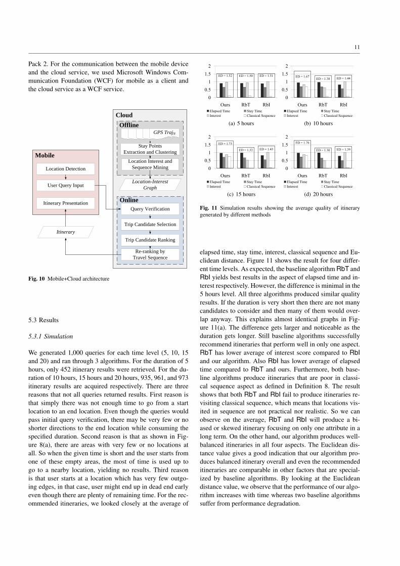
We generated 1,000 queries for each time level (5, 10, 15and 20) and ran through 3 algorithms. For the duration of 5hours, only 452 itinerary results were retrieved. For the du-ration of 10 hours, 15 hours and 20 hours, 935, 961, and 973itinerary results are acquired respectively. There are threereasons that not all queries returned results. First reason isthat simply there was not enough time to go from a startlocation to an end location. Even though the queries wouldpass initial query verification, there may be very few or noshorter directions to the end location while consuming thespecified duration. Second reason is that as shown in Fig-ure 8(a), there are areas with very few or no locations atall. So when the given time is short and the user starts fromone of these empty areas, the most of time is used up togo to a nearby location, yielding no results. Third reasonis that user starts at a location which has very few outgo-ing edges, in that case, user might end up in dead end earlyeven though there are plenty of remaining time. For the rec-ommended itineraries, we looked closely at the average of

0

0.5

1

1.5

2

Ours RbT RbI

Elapsed Time Stay Time

Interest Classical Sequence

ED = 1.51ED = 1.52 ED = 1.50

(a) 5 hours

0

0.5

1

1.5

2

Ours RbT RbI

Elapsed Time Stay Time

Interest Classical Sequence

ED = 1.67ED = 1.38 ED = 1.44

(b) 10 hours

0

0.5

1

1.5

2

Ours RbT RbI

Elapsed Time Stay Time

Interest Classical Sequence

ED = 1.73

ED = 1.32 ED = 1.43

(c) 15 hours

0

0.5

1

1.5

2

Ours RbT RbI

Elapsed Time Stay Time

Interest Classical Sequence

ED = 1.76

ED = 1.30 ED = 1.39

(d) 20 hours

Fig. 11 Simulation results showing the average quality of itinerarygenerated by different methods

elapsed time, stay time, interest, classical sequence and Eu-clidean distance. Figure 11 shows the result for four differ-ent time levels. As expected, the baseline algorithm RbT andRbI yields best results in the aspect of elapsed time and in-terest respectively. However, the difference is minimal in the5 hours level. All three algorithms produced similar qualityresults. If the duration is very short then there are not manycandidates to consider and then many of them would over-lap anyway. This explains almost identical graphs in Fig-ure 11(a). The difference gets larger and noticeable as theduration gets longer. Still baseline algorithms successfullyrecommend itineraries that perform well in only one aspect.RbT has lower average of interest score compared to RbIand our algorithm. Also RbI has lower average of elapsedtime compared to RbT and ours. Furthermore, both base-line algorithms produce itineraries that are poor in classi-cal sequence aspect as defined in Definition 8. The resultshows that both RbT and RbI fail to produce itineraries re-visiting classical sequence, which means that locations vis-ited in sequence are not practical nor realistic. So we canobserve on the average, RbT and RbI will produce a bi-ased or skewed itinerary focusing on only one attribute in along term. On the other hand, our algorithm produces well-balanced itineraries in all four aspects. The Euclidean dis-tance value gives a good indication that our algorithm pro-duces balanced itinerary overall and even the recommendeditineraries are comparable in other factors that are special-ized by baseline algorithms. By looking at the Euclideandistance value, we observe that the performance of our algo-rithm increases with time whereas two baseline algorithmssuffer from performance degradation.

12

5.3.2 User Study

Itinerary at equilibrium: For 10 participants’ 30 queriesover Beijing area, we observed the equilibrium of differentitinerary attributes in our algorithm compared to the base-line algorithms. As we observed from the simulation, ouralgorithm produces an itinerary that is well-balanced in thefour attributes. So in this user study, we show that our al-gorithm produces results that are nearly equal to the base-lines which specialize in a certain single attribute. For in-stance, we check how our result compares with RbT pro-duced itinerary in terms of elapsed time, stay time and traveltime. Since RbT produces results that maximize the timeuse, we wanted to check whether the difference user per-ceives is significant compare to our result which produceswell-balanced and nearly close result. Table 3 shows thecomparison between our algorithm and RbT in terms of timeuse. As the T-test reveals that there is no significant advan-tage in perceived elapsed time, stay time, and travel timefrom using RbT over ours. Actually, in 30 queries in ouruser study, itineraries recommended by our algorithm re-ceived higher scores compared to that of RbT. Similarly, wecompared our result in terms of locations interest includedin the itinerary as shown in Table 3. Here again our resultsscored higher and the T-test reveals that there is no signif-icant advantage in perceived interest from using RbI overours.

Attributes Ours Rank-by-Time T-testElapsed Time 3.97 3.67 p 6≤ 0.01

Stay and Travel Time 3.60 3.27 p 6≤ 0.01Attribute Ours Rank-by-Interest T-testInterest 3.27 2.92 p 6≤ 0.01

Table 3 Comparison of temporal and location interest attributes

Ranking ability: Table 4 shows the ranking ability ofdifferent methods measured by MAP (Mean Average Preci-sion). MAP for a set of queries is the mean of the averageprecision scores for each query.

MAP =∑

Qq=1 AveP(q)

Q(18)

where Q is the number of queries. We treat 30 recommendeditineraries as a ranked retrieval run. In our experiment, MAPstands for the mean of the precision score after each relevantitinerary is retrieved, which is determined by users. We con-sider an itinerary relevant, if its relevance score is 1 or 2 asshown in Table 2. For 30 itineraries generated for three dif-ferent methods, the result is shown in Table 5. Our methodshowed a better performance compared to other baselines.

Measurement Ours Rank-by-Time Rank-by-InterestMAP 0.684 0.622 0.645

Table 4 Ranking ability of different methods

5.3.3 Mobile+Cloud Configuration

We compared the time it takes to recommend an itinerary instandard-alone mobile approach (Mobile Only) and cloudapproach (Mobile+Cloud). In Mobile Only, recommenda-tion is operated fully in the mobile phone. Mobile+Cloudhas distributed tasks between the mobile and the cloud. Allcollected trajectories are data mined in offline in a sepa-rate server and the resulting Location-Interest Graph (G) isused in both Mobile Only and Mobile+Cloud modes. Thedata size of Location-Interest Graph (G) is small which onlycontains information on 1) location itself (interest, typicalstaying time) and 2) relationship between locations (typicaltraveling time, classical travel sequence). We measured theprocessing time for three durations (5 hours, 10 hours and15 hours). We did not test with 20 hours, since it took unrea-sonable long time to measure on the mobile side. For eachduration level, 10 unique test queries are used. Figure 12shows the experiment results. ���������������������� ��� �������������� � ���������������������� ���������������������������������� ������������������������������������ ������������ ���������� ����� ��� ��������� ��������������������� ���� ����������������������� ���� ���� �������������������������������� �������������� ���������������������������� ��������������������������������������� ��� ������ ��� ������ !"#$%&%'()$*+,,$#-&!"+#(.",/0&!"+#1(2�������������������� ���34���� ������������������ �����555������������� ���������������������� �����6���5���� ��75������8��������� �������� ����������� �����9������� ����������� ������� ����������:���� ���� ����6:;8����������� � ���������� ������6�� ����������� ���������� ��������������� ��� ����������8�������������� � ������<������ ������� ����������������� ������ ���������= �>������?���6=�?8� ��= �>���������������6=��8��=�?����������� ������ ����� ��� >������������������� � � �������� ��=������������� ������ ����� ��� ���������������� �������������������������������@�����A������ ������������������������ �������� �������� ��������� ������� ������ ����������������������� ������� �������������� ����������������� ������ ����� ����� � ���������� �������� ���������6�� ����������� ��������������� ���� ��� ����������8���� �BCDEFEGHIJKE BLDEMNEGHIJK� � �BODEMFEGHIJK� BPDEQNEGHIJK�RSTIJUEVWEXHLSYUEIKUJESZ[UJ\COUE]JH[H[̂]UWE !"#$%&%'()$*+,,$#-&!"+#(���������� ������_;;����>������������������?���� � ������ ����������� ��������������� ̀.ab.. cd(? ���������������� ���������������������������<����������������������������������� �����>��������������������������������� ������� ����� ������� ������� ���������������� ��� � ���������������������>� ������������������������������������������������ �� �������������� ����� ������� �������� ��������������� ��� � ������������ ���������������������������������������� �������e����� ���� ���� ���f������������� ������� ����6��g�����8����� ��������������������������e����� ���� ����9�������������� ���� ������� �������������� �������������������e����� ���� ���� �� ��� ��� ������������������� �����7���������7�f������>������ ��������������������� ���� ���� � ��������������������������e����� ���� ����<��� ������������>������������>��������������������� ������ ���� ����������������������� �������������� ���� ���������������������������������������������� � ���������������� ���� ������acdahb. cd(?����������������iajdckhl̀ mnldo.(�55������7 9��� =�? =��:� ����?�� �� ��?���������� p� ��� ����������:;�q�����:;�q����7 :;�q����5 55������7 9��� =�? =��:� ����?�� �� ��?���������� p� ��� ����������:;�q���rs :;�q���At :;�q���uu 55������7 9��� =�? =��:� ����?�� �� ��?���������� p� ��� ����������:;�q���sA :;�q���A7 :;�q���uA 55������7 9��� =�? =��:� ����?�� �� ��?���������� p� ��� ����������:;�q���sr :;�q���A5 :;�q���Av� �BCDEFEGHIJK� BLDEMNEGHIJKE�BODEMFEGHIJKERSTIJUEwWExHy]CJSKHZEH\E[zHEC]]JHCOGUKWE� 5�7A{SyUEBKUOD {UK[E|IUJSUK}�����9��� }�����e�p��� 5��5��{SyUEBKUOD {UK[E|IUJSUK}�����9��� }�����e�p���5��5��75{SyUEBySZD {UK[E|IUJSUK}�����9��� }�����e�p��� XHLSYUEBKUOHZPKDE XHLSYUE~ExYHIPEBKUOHZPKDE �EH\E�ZS[SCYExCZPSPC[UKEArs�r�t� ���tus� rus7�uuv�7u�� 75�vtt� ��r��7rs�75s� �A��u�� ur5A�MN�MWNV�EB�DE Q�Ww��EB�DE VN�VwEB�DEur5��57� 75�7u7� rAs���su�5uu� �5�755� u���7A�vtu� r��t�� �stvv�7v��uut� ���7v7� stv�MW�w�EB�DE QWFM�EB�DE QMEB�DE�v�v�t� A�us7� �5A�{CLYUEMWExHy]CJSKHZEJUKIY[KE\HJEMFEGHIJKWEFig. 12 Performance comparison of Mobile+Cloud architecture

In 5 hours, Mobile Only was faster than Mobile+Cloud.This can be explained by the fact that the finding trip can-didate process in shorter duration does not take much time.Since we cannot add many locations nor travel further givenshorter duration. In Mobile Only, it took less than 1 secondto find candidate trips and get the recommended itinerary for5 hours duration. However, in Mobile+Cloud it took coupleof seconds. So even though the actual processing was donemuch faster in the cloud, the time needed for binding themobile client with the WCF service took some time and it

13

also took more time for communication. So in our obser-vation, the cloud approach had at least couple of secondsfor communication. The performance gap is noticeable fortime duration of 10 hours and 15 hours. The longer dura-tion means that there are more number of candidate tripsto find and rank. As shown in Figure 12 (b), the process-ing time for Mobile Only takes about three times longerthan Mobile+Cloud. For some queries, Mobile Only wasfaster, this is due to the fact that the result contains only asmall number of candidates. In 15 hours, the high computa-tion burden on Mobile Only is clear. As shown in Figure 12(c), Mobile Only takes at least few minutes to recommendan itinerary whereas Mobile+Cloud can handle the requestwithin a minute. In comparison, Mobile Only failed to pro-duce results in neither real-time nor interactive time. Sometest queries lasted for over 15 minutes, which is unbearablein real use cases.

5.4 Discussions

Temporal aspects: The length of duration is an interestingattribute to look at. Many participants used duration between6 to 12 hours. It supports our initial assumption that peoplewould not have such a long journey and keep them in a man-ageable size. For shorter duration, the measured quality ofitineraries were less for our algorithm based on Euclideandistance of attributes. Conversely, two baseline algorithmsproduced the best quality at the shorter duration and recom-mended less efficient itineraries with longer duration. In ex-treme cases though, it was possible for baseline algorithmssuch as RbI to recommend an itinerary that only contains acouple of interesting locations without spending all availabletime. However, since duration was used as a stopping condi-tion in selecting candidates, most recommended itinerariesspend good ratio of available time in simulation and in realuser queries alike. Also users were more judgmental of andinterested in traveling time (on average, less than 1 hour)than staying time at locations (on average, greater than 1hour). Therefore, it would be interesting research directionto give a good projection on traveling time including manyoptions of transportation modes.

Location interest and classical sequence. As shown inFigure 11, our algorithm produced a balanced itinerary withhigher classical sequence scores. In algorithmic level, our al-gorithm showed a great performance advantage in terms ofthe four attributes including classical travel sequence. How-ever, in real queries by users it was difficult to measure lo-cation interest and classical travel sequences from the rec-ommended itinerary. Even though an itinerary is composedof many locations and sequences, we only asked the partici-pants to give ratings for the overall location interest and clas-sical sequence. So they gave high score for classical travel

sequences they could find, and gave lower score for any ab-normal sequences that sometimes balances each other out.So this is different from our simulation where each locationinterest and classical travel sequences were accumulated togive the overall score. In our current algorithm, we only con-sider increment of score for location interest and any clas-sical travel sequences found, yet in the real situation, wemight need to decrease score or give penalties for totallyuninteresting locations and awkward sequences. This is an-other research direction that can help recommend a betteritinerary by avoiding (possibly known) bad sequences in thefirst place.

Mobile deployment. Table 5 shows performance com-parison results for 15 hours duration. When we closely ob-serve the query that took the longest time to process, we cannotice that those queries resulted in a very large number ofinitial candidates. Also the query with the shortest process-ing time deals with a very small number of initial candidates.So we have two heuristics that we can use to choose betweenMobile Only and Mobile+Cloud.

Mobile Only Mobile+Cloud CandidatesQ1 367.658 15.847 6472Q2 449.245 20.988 1165Q3 267.207 13.545 4603Q4 1081.038 (L) 27.489 (L) 30734 (L)Q5 460.502 20.242 6375Q6 174.044 10.200 45Q7 123.984 6.181 17899Q8 291.448 15.292 789Q9 1.647(S) 2.517(S) 21 (S)Q10 19.958 3.472 503

Table 5 Recommendation processing time(sec) comparison for 15hours, (L) indicates the longest/largest and (S) indicates the short-est/smallest.

(1) If the time duration is large (qt > 5 hr), we are betteroff to use Mobile+Cloud. Only use Mobile Only for a veryshort duration, since Mobile+Cloud approach has a reason-ably low lower-bound around 2 seconds to match the perfor-mance of mobile approach.

(2) If we know that the query will generate many candi-date trips, then we should use Mobile+Cloud. We can sim-ply check this by counting the number of outgoing edges ofstart location and incoming edges of end location. If thesenumbers are large then the number of candidate trips will belarge also.

Alternative sources of digital trails. In our work weused GPS trajectories as the primary means of digital trailsgenerated by users. Taking this idea further, different combi-nations of digital trails can be incorporated for cross check-ing and improving accuracy of the work proposed here. Thenotable and relevant research domain deals with many re-

14

sources found on the web, especially with user comments[27], geo-tagged multimedia such as Flickr photo streams[4][10] and social network services. For end-user side, [24]proposed mashup paradigm in ubiquitous computing envi-ronment through augmented reality where users can pro-duce content and services attached to real world objects. Re-cently Zhang et al. proposed ”social and community intelli-gence (SCI)” to learn from different patterns of individual,group and societal behaviors detected pervasive sensing andcontext-aware computing environment [26].

Limitation. There are number of limitations in our ap-proach. Since our method relies on user-generated GPS tra-jectories, it is important to collect a good data set. Our datais collected by highly motivated and active volunteers as atrusted source, but in real case including different Web 2.0check-in sites, many user-generated GPS trajectories needto be validated. In our current setting, we use stay pointdetection, stay point clustering and location clustering toremove much noise, but stronger means of detecting ab-normities in the source are required. One of our goal initinerary recommendation was to minimize user interven-tion and automate the process with a simple query. However,to get a more personalized and accurate itinerary beyonditinerary recommendation for new travelers, we need to con-sider various contextual information such as different trans-portation modes and ranges of itineraries. In our previousworks[30][31] transportation mode is considered, but theseare not fully incorporated with itinerary recommendation.Also our itinerary recommendation is tested in city-level,but scalability is another direction for future work. Lastly,semantic aspects need to be combined with locations, sincesome locations have opening and closing hours and may beaffected by the contextual situations such as weather con-ditions, traffic jams, festivities, and crowded holiday peri-ods. Our current itinerary recommendation framework canbe improved by considering these issues.

6 Conclusion

In this paper, user-generated digital trails such as GPS trajec-tories are collected and data mined to extract collective so-cial intelligence. Specifically we used GPS trajectories from125 users to build Location-Interest Graph which reflectstravel history and experience of travel experts and active res-idents. By using Location-Interest Graph and the proposeditinerary model, itinerary is recommended according to auser-supplied query. To recommend an efficient itinerary, wecollectively used four attributes mined from out data set togenerate balanced and practical itineraries. When comparedto baselines RbT and RbI, our proposed method was com-petitive in both time use and interest level and outperformedbaselines in classical travel sequence aspect in both simula-tion mode and through user study. Especially, the best per-

formance of our method was observed in the longer dura-tion. Also we found that computation intensive task suchas social itinerary recommendation can be distributed ef-fectively in Mobile+Cloud architecture for practical mobileadaptation and application deployment.

For future work, we would like to give better indicationsin traveling time between locations by differentiating useof transportation modes. Also hybrid itinerary recommen-dation based on other sources of digital trails and contextualinformation such as geo-tagged multimedia and check-insare potential works.

Acknowledgements This research was supported by Ministry of Cul-ture, Sports and Tourism (MCST) and Korea Creative Content Agency(KOCCA), under the Culture Technology(CT) Research & Develop-ment Program 2011 and Microsoft Research Asia (MSRA). We alsolike to acknowledge anonymous reviewers for providing invaluablecomments and suggestions.

References

1. Ardissono L, Goy A, Petrone G, Segnan M (2005) A multi-agentinfrastructure for developing personalized web-based systems. ACMT Internet Techn 5:47–69. doi:10.1145/1052934.1052936

2. Ashbrook D, Starner T (2003) Using GPS to learn significant lo-cations and predict movement across multiple users. Pers UbiquitComput 7:275–286. doi:10.1007/s00779-003-0240-0

3. Cao L, Krumm J (2009) From GPS traces to a routableroad map. In: Proceedings of GIS 2009, pp 3–12.doi:10.1145/1653771.1653776

4. Chodhury MD, Feldman M, Amer-Yahia S, Golbandi N, Lem-pel R, Yu C (2010) Automatic construction of travel itineraries us-ing social breadcrumbs. In: Proceedings of HT 2010, pp 35–44.doi:10.1145/1810617.1810626

5. Dunstall S, Horn MET, Kilby P, Krishnamoorthy M, Owens B, SierD, Thiebaux S (2003) An automated itinerary planning system forholiday travel. Infor Technol Tour 6:195–210

6. GeoLife GPS Trajectories (2010). http://bit.ly/bd78Rt,http://bit.ly/gY2JHq

7. Giannotti F, Nanni M, Pinelli F, Pedreschi D (2007) Trajec-tory pattern mining. In: Proceedings of KDD 2007, pp 330–339.doi:10.1145/1281192.1281230

8. Girardin F, Calabrese F, Flore F, Ratti C, Blat J (2008) Digital foot-printing: uncovering tourists with user-generated content. IEEE Per-vas Comput 7:36–43. doi:10.1109/MPRV.2008.71

9. Haversine formula (2010), http://en.wikipedia.org/wiki/Haversineformula. Accessed 24 November 2010

10. Hollenstein L, Purves R (2010) Exploring place through user-generated content: using Flickr to describe city cores. J Spat InforSci 1:21–48. doi:10.5311/JOSIS.2010.1.3

11. Huang Y, Bian L (2009) A Bayesian network and ana-lytic hierarchy process based personalized recommendations fortourist attractions over the Internet. Expert Syst Appl 36:933–943.doi:10.1016/j.eswa.2007.10.019

12. Kim J, Kim H, Ryu JH (2009) TripTip: a trip planning service withtag-based recommendation. In: Proceedings of CHI EA, pp 3467–3472. doi:10.1145/1520340.1520504

13. Krumm J (2010) Where will they turn: predicting turn pro-portions at intersections. Pers Ubiquit Comput 14:591–599.doi:10.1007/s00779-009-0248-1

14. Kumar P, Singh V, Reddy D (2005) Advanced traveler infor-mation system for Hyderabad city. IEEE T Intell Transp 6:26–37.doi:10.1109/TITS.2004.838179

15

15. Li Q, Zheng Y, Xie X, Chen Y, Liu W, Ma WY (2008) Mining usersimilarity based on location history. In: Proceedings of GIS 2008, pp.1–10. doi:10.1145/1463434.1463477

16. Monreale A, Pinelli F, Trasarti R, Giannotti F (2009) WhereNext:a location predictor on trajectory pattern mining. In: Proceedings ofKDD 2009, pp. 637–646. doi:10.1145/1557019.1557091

17. Stabb S, Werther H, Ricci F, Zipf A, Gretzel U, Fesenmaier D,Paris C, Knoblock C (2002) Intelligent systems for tourism. IEEEIntell Syst 17:53–66. doi:10.1109/MIS.2002.1134362

18. Spherical law of cosines (2010), http://en.wikipedia.org/wiki/Spherical law of cosines. Accessed 24 November 2010

19. Suh Y, Shin C, Woo W (2009) A Mobile Phone Guide: Spatial,Personal, and social experience for cultural heritage. IEEE T Con-sum Electr 55:2356–2364. doi:10.1109/TCE.2009.5373810

20. Suh Y, Shin C, Dow S, MacIntyre B, Woo W (2010) Enhancingand evaluating users’ social experience with a mobile phone guideapplied to cultural heritage. Pers Ubiquit Comput Online First:1–17.doi:10.1007/s00779-010-0344-2

21. Tai CH, Yang DN, Lin LT, Chen MS (2008) Recommending per-sonalized scenic itinerary with geo-tagged photos. In: Proceedingsof ICME 2008, pp. 1209–1212. doi:10.1109/ICME.2008.4607658

22. Takeuchi Y, Sugimoto M (2009) A user-adaptive city guide sys-tem with an unobtrusive navigation interface. Pers Ubiquit Comput13:119–132, doi:10.1007/s00779-007-0192-x

23. Werthner H (2003) Intelligent systems in travel and tourism. In:Proceedings of IJCAI 2003, pp. 1620–1628

24. Yoon H, Woo W (2009) CAMAR Mashup: Empowering end-userparticipation in U-VR environment. In: Proceedings of ISUVR 2009,pp. 33–36. doi:10.1109/ISUVR.2009.22

25. Yoon H, Zheng Y, Xie X, Woo W (2010) Smart itinerary recom-mendation based on user-generated GPS trajectories. In: Proceedingsof UIC 2010, pp. 19–34. doi:10.1007/978-3-642-16355-5 5

26. Zhang D, Guo B, Li B, Yu Z (2010) Extracting social and com-munity intelligence from digital footprints: an emerging researcharea. In: Proceedings of UIC 2010, pp. 4–18. doi:10.1007/978-3-642-16355-5 4

27. Zheng VW, Zheng Y, Xie X, Yang Q (2010) Collaborative locationand activity recommendations with GPS history data. In: Proceed-ings of WWW 2010, pp. 1029–1038. doi:10.1145/1772690.1772795

28. Zheng VW, Cao B, Zheng Y, Xie X, Yang Q (2010) Collaborativefiltering meets mobile recommendation. In: Proceedings of AAAI2010, pp. 238–241

29. Zheng Y, Wang L, Zhang R, Xie X, Ma WY (2008) GeoLife: man-aging and understanding your past life over maps. In: Proceedings ofMDM 2008, pp. 211–212. doi:10.1109/MDM.2008.20

30. Zheng Y, Li Q, Chen Y, Xie X, Ma WY (2008) Understandingmobility based on GPS data. In: Proceedings of Ubicomp 2008, pp.312–321. doi:10.1145/1409635.1409677

31. Zheng Y, Liu L, Wang L, Xie X (2008) Learning trans-portation mode from raw GPS data for geographic applicationson the web. In: Proceedings of WWW 2008, pp. 247–256.doi:10.1145/1367497.1367532

32. Zheng Y, Chen Y, Xie X, Ma WY (2009) GeoLife2.0: a location-based social networking service. In: Proceedings of MDM 2009, pp.357–358. doi:10.1109/MDM.2009.50

33. Zheng Y, Zhang L, Xie X, Ma WY (2009) Mining interesting lo-cations and travel sequences from GPS trajectories. In: Proceedingsof WWW 2009, pp. 791–800. doi:10.1145/1526709.1526816

34. Zheng Y, Zhang L, Xie X, Ma WY (2009) Mining correlation be-tween locations using human location history. In: Proceedings of GIS2009, pp. 472–475. doi:10.1145/1653771.1653847

35. Zheng Y, Chen Y, Li Q, Xie X, Ma WY (2010) Understandingtransportation modes based on GPS data for web applications. ACMTrans Web 4:1–36. doi:10.1145/1658373.1658374

36. Zheng Y, Xie X, Ma WY (2010) GeoLife: a collaborative socialnetworking service among user, location and trajectory. IEEE DataEng Bull 33:32–39

37. Zheng Y, Xie X (2011) Learning travel recommendations fromuser-generated GPS traces. ACM Trans Intell Syst Technol 2:1–29.doi:10.1145/1889681.1889683

38. Zheng Y, Zhang L, Ma Z, Xie X, Ma WY (2011) Recommend-ing friends and locations based on individual location history. ACMTrans Web 5:1–44. doi:10.1145/1921591.1921596