smip14 seminar proceedings accounting for topographic effects in ground motion ... · pdf...

SMIP14 Seminar Proceedings

13

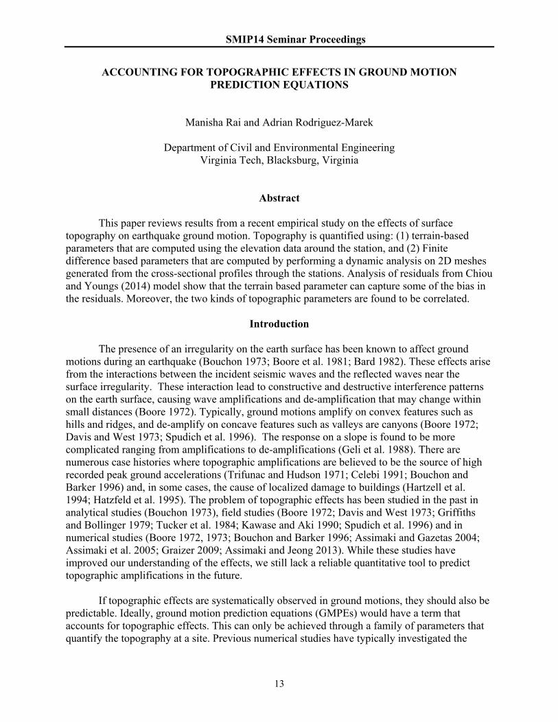
ACCOUNTING FOR TOPOGRAPHIC EFFECTS IN GROUND MOTION PREDICTION EQUATIONS

Manisha Rai and Adrian Rodriguez-Marek

Department of Civil and Environmental Engineering Virginia Tech, Blacksburg, Virginia

Abstract This paper reviews results from a recent empirical study on the effects of surface

topography on earthquake ground motion. Topography is quantified using: (1) terrain-based parameters that are computed using the elevation data around the station, and (2) Finite difference based parameters that are computed by performing a dynamic analysis on 2D meshes generated from the cross-sectional profiles through the stations. Analysis of residuals from Chiou and Youngs (2014) model show that the terrain based parameter can capture some of the bias in the residuals. Moreover, the two kinds of topographic parameters are found to be correlated.

Introduction

The presence of an irregularity on the earth surface has been known to affect ground

motions during an earthquake (Bouchon 1973; Boore et al. 1981; Bard 1982). These effects arise from the interactions between the incident seismic waves and the reflected waves near the surface irregularity. These interaction lead to constructive and destructive interference patterns on the earth surface, causing wave amplifications and de-amplification that may change within small distances (Boore 1972). Typically, ground motions amplify on convex features such as hills and ridges, and de-amplify on concave features such as valleys are canyons (Boore 1972; Davis and West 1973; Spudich et al. 1996). The response on a slope is found to be more complicated ranging from amplifications to de-amplifications (Geli et al. 1988). There are numerous case histories where topographic amplifications are believed to be the source of high recorded peak ground accelerations (Trifunac and Hudson 1971; Celebi 1991; Bouchon and Barker 1996) and, in some cases, the cause of localized damage to buildings (Hartzell et al. 1994; Hatzfeld et al. 1995). The problem of topographic effects has been studied in the past in analytical studies (Bouchon 1973), field studies (Boore 1972; Davis and West 1973; Griffiths and Bollinger 1979; Tucker et al. 1984; Kawase and Aki 1990; Spudich et al. 1996) and in numerical studies (Boore 1972, 1973; Bouchon and Barker 1996; Assimaki and Gazetas 2004; Assimaki et al. 2005; Graizer 2009; Assimaki and Jeong 2013). While these studies have improved our understanding of the effects, we still lack a reliable quantitative tool to predict topographic amplifications in the future.

If topographic effects are systematically observed in ground motions, they should also be

predictable. Ideally, ground motion prediction equations (GMPEs) would have a term that accounts for topographic effects. This can only be achieved through a family of parameters that quantify the topography at a site. Previous numerical studies have typically investigated the


14

effects of site geometry on input ground motions through parametric studies on simple parameters (e.g., slope gradient, slope height and width; Boore 1972; Ashford et al. 1997). Any parameter that affects the ground motion at a site is valid parameter that can be potentially included in a GMPE to model topographic effects. However, a good parameter is one that is able to statistically reduce the bias in the prediction of ground motions. In a recent paper (Rai et al 2014) we looked at some parameters derived from the terrain elevation. We found that two of these parameters (relative elevation and smoothed curvature) can reduce the biases in the predictions in GMPEs. In the current work, we will first briefly review these parameters and their effects on reducing bias in GMPEs and then continue to explore another parameter that is based on the results of the finite difference analysis of 2D models based the geometry at the station. The results from these analyses are only preliminary and further study is currently under progress.

Methodology

The current GMPEs do not account for topographic effects. The residuals from these

models are thus expected to carry a systematic bias with respect to topography. To test this, we look at the residual component that reflects repeatable site effects (which are obtained by partitioning the residuals), and evaluate trends in these residuals with respect to topographic parameters at each station. The following sections discuss the partition of residuals and the parameterization of topography.

Residual partitioning

The residuals from a GMPE prediction are split into inter-event and intra-event residuals

as shown: (1)

where is the natural log of the observed spectral acceleration (Sa) minus the natural log of the predicted Sa; is the event term (or inter-event residual) which is the residual component that is common to all the sites recording that event; and is the intra-event residual which is the residual component at a site after removing from the total residual. The intra-event residuals can be further partitioned as follows:

2 (2)

where 2 is the site residual and is the site and event corrected residual. The site term ( 2 ) can be thought of as the average residual at a site after correcting for the event terms. As topographic effects are site effects, topography related bias is expected to be present in the site residuals ( 2 ). All the residual components in Eqs. (1) and (2) are assumed to be independent zero-mean normally distributed variables. A description of these residual components and their variances are given in Table 1.

In this study, we use the intra-event residuals from the Chiou and Youngs (2014) NGA

West2 ground motion model to obtain the site terms ( 2 ). The Chiou and Youngs (2014) ground motion dataset has recordings from 300 earthquakes of magnitude 3 and higher. The


15

recordings were made at 3208 ground motion recording stations located across California, Alaska, Japan, Taiwan, China, Turkey, Italy, Iran, and New Zealand. To get a good estimate of 2 at each station, only stations that have at least three recording are included in the study.

Such a filtering should not introduce any systematic bias with respect to topography in the data, as the elimination criterion is independent of topography.

Table 1: Description of residual components

Residual

Component Description

Standard

deviation

Inter-event residual

Intra-event residual

δS2S Site-to-site residual

δWS Single- site within-event residual

This constraint resulted in a total of 9,195 ground motions and 798 stations located in

California and Japan (Figure 1). The magnitude-distance distribution of the records in this dataset is shown in Figure 2. The dataset consists of ground motion residuals at 105 spectral periods from 0.01 s to 10 s.

Figure 1: Locations of earthquake hypocenters and recording stations are shown for the ground motions used in the study from California (left) and Japan (right). Only stations with at least 3 recordings are considered. Due to these criteria, only ground motions from California and Japan were selected.


16

Figure 2: Earthquake magnitudes are plotted with the distance to the recording stations for the ground motions used in the study.

Topographic parameters In a previous study (Rai et al, 2014), we looked at the topographic parameters that were

computed solely using the elevation data around the station. We refer to such parameters as geometry-based parameters. In the current work, we compute another set of topographic parameters that are based on the finite difference analysis. Both these parameters are explained here. Geometry based parameters

The two geometry based parameters we studied are Relative Elevation and Smoothed

Curvature. Both these parameters are computed using the elevation data around the station location. All the computations are done in ArcGIS (ESRI, 2011).

Relative elevation is computed for each cell of the digital elevation model (DEM) by

taking the difference of elevation at the cell and the mean elevation of the cells within a neighborhood of the cell. A circular neighborhood is used for computing mean and the diameter of the circle is referred to as the scale parameter. Relative elevation calculated at a scale parameter value of is referred to as . A positive value means that the elevation of the cell is higher than the mean elevation in the neighborhood; a negative value means that the elevation of the cell is lower than the mean elevation in the neighborhood and a value of zero means that the station is located in a region of uniform slope. For this reason, is effective in highlighting features such as ridges ( 0), valleys ( 0) and plains/slopes ( 0). An example of for D = 500 m, 1000 m and 2000 m is shown in Figure 3.


17

a) b)

c) d)

Figure 3: The effect of increasing the scale parameter D on relative elevation is demonstrated. Shown here are a) elevation raster, and relative elevation rasters at a scale of b) 500 m, c) 1000 m, and d) 2000 m. Note that at a scale of 500 m, finer features are visible. As the scale is increased, some of the finer features diminish, and broader features become more prominent.

Smoothed curvature ( ) is computed using the curvature tool in ArcGIS. First, the

elevation data is smoothed using a certain window size, also referred to as the scale-parameter. This smoothed elevation data is then input into the curvature tool, and the output raster is referred to as the smoothed curvature ( ). Different scales ranging from 60 m to 600 m were used to study the effects of smoothing on the curvature values.

Finite difference analysis based parameters

The goal of this parameterization scheme is to obtain a set of topographic parameters that

are based on the results of numerical analyses conducted using 2D cross-sectional profiles at the station. The output from the analyses will be time-histories at the ground surface. The time history at the location of the station can be used to compute parameters such as the ratio of at the site and at an equivalent site with no topography. Reproducing the exact dynamic response of the site is not a concern as these parameters will be used as independent variables in a prediction exercise where it is advantageous to keep the parameters simple so that they can be


18

easily computed for any site in the future. For this reason, we only use an elastic soil, with simple soil properties.

For each station in the NGAWest2 dataset, 2D cross-sectional profiles are obtained at

azimuths of 0, 30, 60, 90, 120 and 150 degrees from the north, a total of 6 profiles for each station. Multiple sections are used to capture the potential for directional 3D topographic effects. The elevation data for the profile is discretized at 30 m interval to match the approximate 30 m resolution of the DEM. The total length of each profile is 2000 m, and the station is located at the center of each profile (Figure 4). The elevation at the site is subtracted from each of the elevation values in a profile such that in the resulting profile, all the stations are always located at an elevation of 0 m. This step is important because we want to keep all the stations at the same height from the base in the resulting finite different mesh. This will ensure that all the stations have the same 1-D resonant periods, and that we only capture topographic effects in the numerical analysis.

Figure 4: 3D terrain around a site (left) and cross-sectional profiles across the station in 6 different directions (right) are shown. The station is located at x = 0, y = 0.

A 2000 m by 2000 m finite difference mesh is generated in FLAC 5.0 (Itasca Consulting

Group, 2005) with a grid size of 25 m in both the x and y directions. The grid is assigned the following soil properties: mass density ρ = 2 Mg/m3, Poisson’s ratio = 1/3, Vs = 500 m/s (Bouckovalas and Papadimitriou 2005; Tripe et al. 2013) and a target damping ratio of 5% using Raleigh damping. Once the grid is generated, the top surface of the grid is distorted to fit the shape of the profile. The base of the mesh is treated as infinite and to model it in FLAC, quiet boundaries are applied at the base of each model in both x and y directions. To minimize reflections from the lateral boundaries, free field boundaries are applied to both the lateral boundaries. A schematic illustration of the mesh and the boundary conditions are shown in Figure 5. Note that the resulting depth to the base of the mesh is same for all the stations.


19

Figure 5: Schematic illustration of the finite difference model used for the analysis at a station. The model uses a realistic topographic cross-section profile at the top. The station is located at the surface, equidistant from both the lateral edges. The height of stations from the base is same for all stations. Free-field boundary condition is applied to the lateral boundaries and quiet boundary conditions are applied at the base.

As the boundaries are quiet, instead of applying accelerations as input, a time history of

shear stress is applied (Itasca Consulting Group, 2005). These stresses are a factor of velocity (Itasca Consulting Group, 2005). The input velocity time history used in the study is a tapered sine-sweep wave. The velocity time history is chosen such that the resulting acceleration time history has a PGA of 1 m/s2 (Figure 6). The input motion consists of frequencies up to 2 Hz .

a) b)

Figure 6: Input a) acceleration and b) velocity time histories for the original and base line corrected motion.


20

The 2 Hz frequency limit is chosen to restrict the number of zones in the mesh (and consequently the computational time) as the maximum mesh dimension is inversely proportional to the highest frequency to be modelled correctly. The total duration of the input motion is 20 s. Output time histories are recorded at each of the grid points on the top surface of the mesh. A similar analysis is conducted using a flat surface at the top (1D analysis), and the results from the 1D analysis (the free field response) is used to normalize the response obtained from the 2D analyses.

Spectral accelerations are computed using the output time histories at the location of the station (x = 0, y = 0) for each of the 6 orientations. These values are normalized with values from the 1D case. The log of minimum, maximum, and average values of the normalized

from the 6 orientations are the topographic parameters for the station. We refer to these parameters as Spectral Amplification Ratio ( , , ). The relationship between (T = 0.5 s) for all the 6 orientations and for the stations in the dataset is shown in Figure 7.

Figure 7: values for T = 0.5 s are plotted with for the stations in the NGAWest2 dataset. A moving average of the terms computed using local regression (loess) is also shown. A high degree of linear correlation is observed between the two parameters.

There is a high linear correlation between the two parameters. At other periods, similar

relationship is observed between the two parameters. This is an interesting finding in two ways: first, it validates the usefulness of the parameter to predict topographic effects; second, this might probably imply that a complicated numerical analysis may not necessarily be required to make predictions about topographic effects in future earthquakes. A simple parameter based on elevation data might just be sufficient to estimate the effects.


21

Results

The site residuals are compared with the topographic parameters obtained in the previous steps. Here we review some of the results from the residual analysis using the geometry based parameters. We will also present some preliminary results from the finite difference analysis.

Geometry based parameters

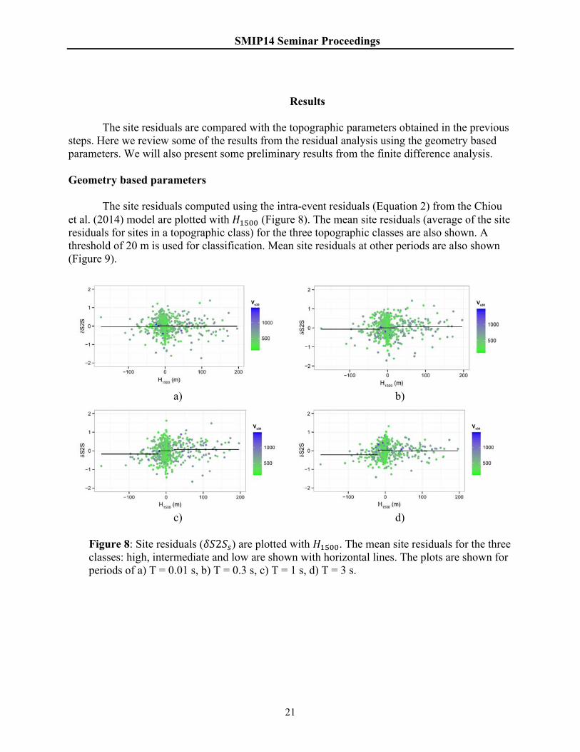
The site residuals computed using the intra-event residuals (Equation 2) from the Chiou

et al. (2014) model are plotted with (Figure 8). The mean site residuals (average of the site residuals for sites in a topographic class) for the three topographic classes are also shown. A threshold of 20 m is used for classification. Mean site residuals at other periods are also shown (Figure 9).

a) b)

c) d)

Figure 8: Site residuals ( 2 ) are plotted with . The mean site residuals for the three classes: high, intermediate and low are shown with horizontal lines. The plots are shown for periods of a) T = 0.01 s, b) T = 0.3 s, c) T = 1 s, d) T = 3 s.


22

Figure 9: Mean site residual for high, low and intermediate sites are shown at different periods. A scale of 1500 m and a threshold of 20 m were used for the classification.

Analysis of variance (ANOVA) is used to test the statistical significance of differences in

the mean site residuals for the three topographic classes. A pair-wise t-test is also performed to test the significance of the difference in mean residual between different pairs of class. A statistical significance is assumed at 95% or for p-values less than 0.05 (i.e., the probability that the differences are due to random chance is less than 5 %). The p-values from ANOVA are below 0.05 levels for periods between 0.32 s and 10 s. The pairwise Tukey’s t-tests show that the difference of mean site residual for intermediate and high lying stations is significant only between periods of 0.38 s to 0.75 s, the difference between low lying and high lying stations are statistically significant for periods greater than 0.30 s, and the difference between low and intermediate stations are significant for periods greater than 0.50 s. The analysis showed that the parameter was able to capture the bias in the residuals and that it is possible to come up with parameters that can be included in the GMPE to reduce biases.

Finite difference based parameter

The site residuals computed above are plotted with at the same period (Figure

10). To check for bias in residuals with respect to values, stations were divided into three classes based on the value at the station. A threshold of 0.5 is used for classification such that station with > 0.5 are classified as high, < - 0.5 are classified as low and the stations with in between -0.5 and 0.5 are classified as intermediate, where denotes the standard deviation of the values. The plot shows a bias in the residuals with respect to the parameter but the trends are less pronounced than those observed in the case of relative elevation parameter. These results are preliminary and additional research is being done to test the significance of the differences observed. Also, various other finite difference based parameters are currently being studied.


23

Figure 10: Site residuals ( 2 ) are plotted with at the same period. The plots are shown for periods of a) T = 0.5 s, b) T = 0.8 s, c) T = 1 s, d) T = 3 s. Plots for periods less than 0.5 s are not shown due to expected numerical distortion of higher frequencies.

Conclusions

The effects of surface topography on earthquake ground motion were studied using the

residuals from Chiou and Young (2014) NGAWest2 datasets. The trends in ground motion residuals were evaluated with respect to topographic parameters. Two kinds of topographic parameters were studies; terrain based and finite difference based. Terrain based parameters were computed using the elevation data at the station. Finite difference based parameters were computed using the output time histories at the station from dynamic analyses using finite differences. The analyses were conducted using meshes that were deformed at the surface to fit the shape of the cross-sectional profile at the station and subjecting the mesh to a tapered sine-sweep input motion. For each station, cross-sectional profiles in 6 different directions were used.

We found that the terrain based parameters were able to predict some of the trends in the

ground motion residuals and they can potentially reduce biases in GMPEs. We also found a high linear correlation between the terrain based parameter and the finite difference based parameter. This finding validates the usefulness of the terrain based parameter, which might not be an intuitive parameter at first. This also shows that a numerical analysis will not necessarily be required to make predictions about ground motions in future earthquakes. It is important to note that this is a work under progress and that some results are only preliminary.


24

References

Ashford, S. A., Sitar, N., Lysmer, J., and Deng, N. (1997). “Topographic effects on the seismic response of steep slopes.” Bulletin of the Seismological Society of America, 87(3), 701–709.

Assimaki, D., and Gazetas, G. (2004). “Soil and topographic amplification on canyon banks and the 1999 Athens earthquake.” Journal of earthquake engineering, 8(01), 1–43.

Assimaki, D., and Jeong, S. (2013). “Ground-Motion Observations at Hotel Montana during the M 7.0 2010 Haiti Earthquake: Topography or Soil Amplification?” Bulletin of the Seismological Society of America, 103(5), 2577–2590.

Assimaki, D., Kausel, E., and Gazetas, G. (2005). “Soil-Dependent Topographic Effects: A Case Study from the 1999 Athens Earthquake.” Earthquake Spectra, 21(4), 929–966.

Bard, P.-Y. (1982). “Diffracted waves and displacement field over two-dimensional elevated topographies.” Geophysical Journal International, 71(3), 731–760.

Boore, D. M. (1972). “A note on the effect of simple topography on seismic SH waves.” Bulletin of the Seismological Society of America, 62(1), 275–284.

Boore, D. M. (1973). “The effect of simple topography on seismic waves: implications for the accelerations recorded at Pacoima Dam, San Fernando Valley, California.” Bulletin of the Seismological Society of America, 63(5), 1603–1609.

Boore, D. M., Harmsen, S. C., and Harding, S. T. (1981). “Wave scattering from a step change in surface topography.” Bulletin of the Seismological Society of America, 71(1), 117–125.

Bouchon, M. (1973). “Effect of topography on surface motion.” Bulletin of the Seismological Society of America, 63(2), 615–632.

Bouchon, M., and Barker, J. S. (1996). “Seismic response of a hill: the example of Tarzana, California.” Bulletin of the Seismological Society of America, 86(1A), 66–72.

Bouckovalas, G. D., and Papadimitriou, A. G. (2005). “Numerical evaluation of slope topography effects on seismic ground motion.” Soil Dynamics and Earthquake Engineering, 25(7-10), 547–558.

Celebi, M. (1991). “Topographical and geological amplification: case studies and engineering implications.” Structural Safety, 10(1), 199–217.

Chiou, B. S.-J., and Youngs, R. R. (2014). “Update of the Chiou and Youngs NGA Model for the Average Horizontal Component of Peak Ground Motion and Response Spectra.” Earthquake Spectra In-Press.

Davis, L. L., and West, L. R. (1973). “Observed effects of topography on ground motion.” Bulletin of the Seismological Society of America, 63(1), 283–298.

ESRI (2011). “ArcGIS Desktop: Release 10.” Redlands, CA.

Geli, L., Bard, P.-Y., and Jullien, B. (1988). “The effect of topography on earthquake ground motion: a review and new results.” Bulletin of the Seismological Society of America, 78(1), 42–63.

Graizer, V. (2009). “Low-velocity zone and topography as a source of site amplification effect on Tarzana hill, California.” Soil Dynamics and Earthquake Engineering, 29(2), 324–332.


25

Griffiths, D. W., and Bollinger, G. A. (1979). “The effect of Appalachian Mountain topography on seismic waves.” Bulletin of the Seismological Society of America, 69(4), 1081–1105.

Hartzell, S. H., Carver, D. L., and King, K. W. (1994). “Initial investigation of site and topographic effects at Robinwood Ridge, California.” Bulletin of the Seismological Society of America, 84(5), 1336–1349.

Hatzfeld, D., Nord, J., Paul, A., Guiguet, R., Briole, P., Ruegg, J.-C., Cattin, R., Armijo, R., Meyer, B., Hubert, A., Bernard, P., Makropoulos, K., Karakostas, V., Papaioannou, C., Papanastassiou, D., and Veis, G. (1995). “The Kozani-Grevena (Greece) Earthquake of May 13, 1995, Ms = 6.6. Preliminary Results of a Field Multidisciplinary Survey.” Seismological Research Letters, 66(6), 61–70.

Itasca Consulting Group, Inc. (2005). “FLAC: fast lagrangian analysis of continua”. User’s manual.

Kawase, H., and Aki, K. (1990). “Topography effect at the critical SV-wave incidence: possible explanation of damage pattern by the Whittier Narrows, California, earthquake of 1 October 1987.” Bulletin of the Seismological Society of America, 80(1), 1–22.

Rai, M., Rodriguez-Marek, A., and Yong, A. (2014). “An empirical model to predict topographic effects in strong ground motion: Study using the California small to medium magnitude earthquake database." To be submitted to Earthquake Spectra.

Spudich, P., Hellweg, M., and Lee, W. H. K. (1996). “Directional topographic site response at Tarzana observed in aftershocks of the 1994 Northridge, California, earthquake: implications for mainshock motions.” Bulletin of the Seismological Society of America, 86(1B), S193–S208.

Trifunac, M. D., and Hudson, D. E. (1971). “Analysis of the Pacoima dam accelerogram—San Fernando, California, earthquake of 1971.” Bulletin of the Seismological Society of America, 61(5), 1393–1411.

Tripe, R., Kontoe, S., and Wong, T. K. C. (2013). “Slope topography effects on ground motion in the presence of deep soil layers.” Soil Dynamics and Earthquake Engineering, 50, 72–84.

Tucker, B. E., King, J. L., Hatzfeld, D., and Nersesov, I. L. (1984). “Observations of hard-rock site effects.” Bulletin of the Seismological Society of America, 74(1), 121–136.


26

smip14 seminar proceedings accounting for topographic effects in ground motion ... · pdf...

Documents