sliding mode observers - historical background and basic introduction
TRANSCRIPT

Sliding mode observers - historical background andbasic introduction
Sarah K. Spurgeon
School of Engineering and Digital ArtsUniversity of Kent, UK
Spring School, Aussois, June 2015
Sarah K. Spurgeon Sliding mode observer

Outline of Presentation
Sliding mode control versus sliding mode observers?
Historical perspective - The Utkin Observer
Tutorial Example
Further historical milestones
Window on the state of the art - Lecture 2
Sarah K. Spurgeon Sliding mode observer
Outline of Presentation
Sliding mode control versus sliding mode observers?
Historical perspective - The Utkin Observer
Tutorial Example
Further historical milestones
Window on the state of the art - Lecture 2
Sarah K. Spurgeon Sliding mode observer
Outline of Presentation
Sliding mode control versus sliding mode observers?
Historical perspective - The Utkin Observer
Tutorial Example
Further historical milestones
Window on the state of the art - Lecture 2
Sarah K. Spurgeon Sliding mode observer
Outline of Presentation
Sliding mode control versus sliding mode observers?
Historical perspective - The Utkin Observer
Tutorial Example
Further historical milestones
Window on the state of the art - Lecture 2
Sarah K. Spurgeon Sliding mode observer

Outline of Presentation
Sliding mode control versus sliding mode observers?
Historical perspective - The Utkin Observer
Tutorial Example
Further historical milestones
Window on the state of the art - Lecture 2
Sarah K. Spurgeon Sliding mode observer

Outline of Presentation
Sliding mode control versus sliding mode observers?
Historical perspective - The Utkin Observer
Tutorial Example
Further historical milestones
Window on the state of the art - Lecture 2
Sarah K. Spurgeon Sliding mode observer

Introduction - The Control Problem
Sliding mode techniques were perhaps originally best knownfor their potential as a robust control method, and evolvedfrom pioneering work in the 1960’s in the former Soviet Union.
Such a sliding mode control is characterised by a suite offeedback control laws and a decision rule. The decision rule,termed the switching function, has as its input some measureof the current system behaviour and produces as an outputthe particular feedback controller which should be used atthat instant in time.
In sliding mode control, VSCS are designed to drive and thenconstrain the system state to lie within a neighbourhood ofthe switching function.
Sarah K. Spurgeon Sliding mode observer

Introduction - The Control Problem
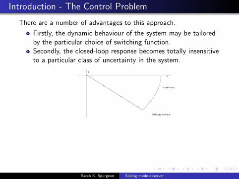
There are a number of advantages to this approach.
Firstly, the dynamic behaviour of the system may be tailoredby the particular choice of switching function.
Secondly, the closed-loop response becomes totally insensitiveto a particular class of uncertainty in the system.
y
y.
trajectory
sliding surface
Figure : A sliding mode
Sarah K. Spurgeon Sliding mode observer

Introduction - The Control Problem
There are a number of advantages to this approach.
Firstly, the dynamic behaviour of the system may be tailoredby the particular choice of switching function.Secondly, the closed-loop response becomes totally insensitiveto a particular class of uncertainty in the system.
y
y.
trajectory
sliding surface
Figure : A sliding mode
Sarah K. Spurgeon Sliding mode observer
The Control Problem - Disadvantages
A disadvantage of the method in the domain of control applicationshas been the necessity to implement a fundamentally discontinuouscontrol signal which, in theoretical terms, must switch with infinitefrequency to provide total rejection of uncertainty. Controlimplementation via approximate, smooth strategies is widelyreported, but in such cases total invariance is routinely lost.
Sarah K. Spurgeon Sliding mode observer

Introduction - The Observer Problem
In contrast, the application of sliding mode methods to theobserver problem is much less mature and has some fundamentallydifferent advantages and disadvantages.
the ability to generate a sliding motion on the error betweenthe measured plant output and the output of the observerensures that a sliding mode observer produces a set of stateestimates that are precisely commensurate with the actualoutput of the plant.
analysis of the average value of the applied observer injectionsignal, the so-called equivalent injection signal, contains usefulinformation about the mismatch between the model used todefine the observer and the actual plant.
the discontinuous injection signals which were perceived asproblematic for many control applications, have nodisadvantages for software based observer frameworks.
Sarah K. Spurgeon Sliding mode observer
A Historical Perspective
System
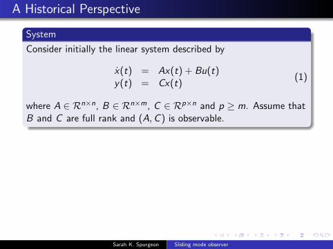
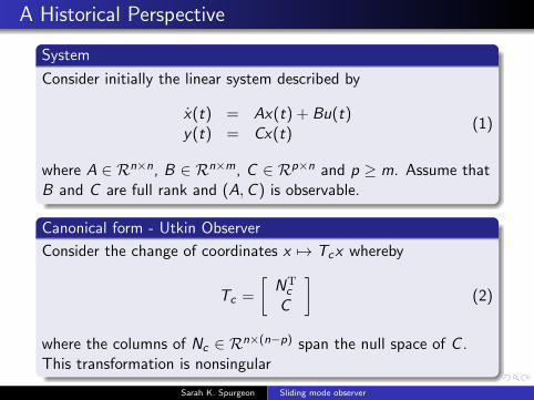
Consider initially the linear system described by
x(t) = Ax(t) + Bu(t)y(t) = Cx(t)
(1)
where A ∈ Rn×n, B ∈ Rn×m, C ∈ Rp×n and p ≥ m. Assume thatB and C are full rank and (A,C ) is observable.
Canonical form - Utkin Observer
Consider the change of coordinates x 7→ Tcx whereby
Tc =
[NTc
C
](2)
where the columns of Nc ∈ Rn×(n−p) span the null space of C .This transformation is nonsingular
Sarah K. Spurgeon Sliding mode observer
A Historical Perspective
System
Consider initially the linear system described by
x(t) = Ax(t) + Bu(t)y(t) = Cx(t)
(1)
where A ∈ Rn×n, B ∈ Rn×m, C ∈ Rp×n and p ≥ m. Assume thatB and C are full rank and (A,C ) is observable.
Canonical form - Utkin Observer
Consider the change of coordinates x 7→ Tcx whereby
Tc =
[NTc
C
](2)
where the columns of Nc ∈ Rn×(n−p) span the null space of C .This transformation is nonsingular
Sarah K. Spurgeon Sliding mode observer
A Historical Perspective
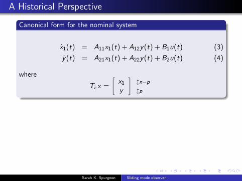
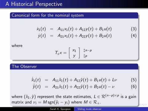
Canonical form for the nominal system
x1(t) = A11x1(t) + A12y(t) + B1u(t) (3)
y(t) = A21x1(t) + A22y(t) + B2u(t) (4)
where
Tcx =
[x1y
]ln−plp
The Observer
˙x1(t) = A11x1(t) + A12y(t) + B1u(t) + Lν (5)
˙y(t) = A21x1(t) + A22y(t) + B2u(t)− ν (6)
where (x1, y) represent the state estimates, L ∈ R(n−p)×p is a gainmatrix and νi = M sgn(yi − yi ) where M ∈ R+.
Sarah K. Spurgeon Sliding mode observer
A Historical Perspective
Canonical form for the nominal system
x1(t) = A11x1(t) + A12y(t) + B1u(t) (3)
y(t) = A21x1(t) + A22y(t) + B2u(t) (4)
where
Tcx =
[x1y
]ln−plp
The Observer
˙x1(t) = A11x1(t) + A12y(t) + B1u(t) + Lν (5)
˙y(t) = A21x1(t) + A22y(t) + B2u(t)− ν (6)
where (x1, y) represent the state estimates, L ∈ R(n−p)×p is a gainmatrix and νi = M sgn(yi − yi ) where M ∈ R+.
Sarah K. Spurgeon Sliding mode observer

A Historical Perspective
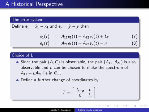
The error system
Define e1 = x1 − x1 and ey = y − y then
e1(t) = A11e1(t) + A12ey (t) + Lν (7)
ey (t) = A21e1(t) + A22ey (t)− ν (8)
Choice of L
Since the pair (A,C ) is observable, the pair (A11,A21) is alsoobservable and L can be chosen to make the spectrum ofA11 + LA21 lie in C−.
Define a further change of coordinates by
T =
[In−p L
0 Ip
]
Sarah K. Spurgeon Sliding mode observer
A Historical Perspective
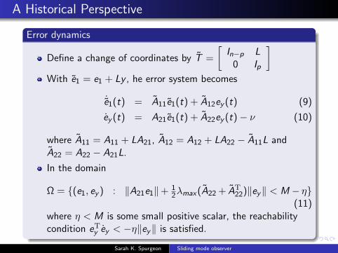
Error dynamics
Define a change of coordinates by T =
[In−p L
0 Ip
]With e1 = e1 + Ly , he error system becomes
˙e1(t) = A11e1(t) + A12ey (t) (9)
ey (t) = A21e1(t) + A22ey (t)− ν (10)
where A11 = A11 + LA21, A12 = A12 + LA22 − A11L andA22 = A22 − A21L.
In the domain
Ω = (e1, ey ) : ‖A21e1‖+ 12λmax(A22 + AT
22)‖ey‖ < M − η(11)
where η < M is some small positive scalar, the reachabilitycondition eTy ey < −η‖ey‖ is satisfied.
Sarah K. Spurgeon Sliding mode observer

A Historical Perspective
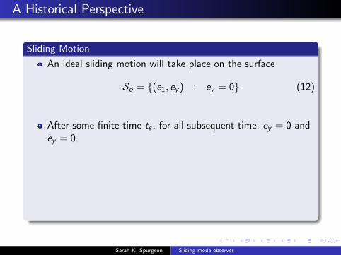
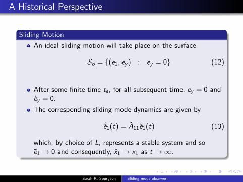
Sliding Motion
An ideal sliding motion will take place on the surface
So = (e1, ey ) : ey = 0 (12)
After some finite time ts , for all subsequent time, ey = 0 andey = 0.
The corresponding sliding mode dynamics are given by
˙e1(t) = A11e1(t) (13)
which, by choice of L, represents a stable system and soe1 → 0 and consequently, x1 → x1 as t →∞.
Sarah K. Spurgeon Sliding mode observer
A Historical Perspective
Sliding Motion
An ideal sliding motion will take place on the surface
So = (e1, ey ) : ey = 0 (12)
After some finite time ts , for all subsequent time, ey = 0 andey = 0.
The corresponding sliding mode dynamics are given by
˙e1(t) = A11e1(t) (13)
which, by choice of L, represents a stable system and soe1 → 0 and consequently, x1 → x1 as t →∞.
Sarah K. Spurgeon Sliding mode observer

Tutorial Example
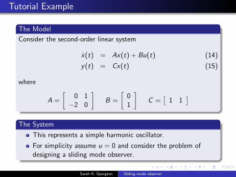
The Model
Consider the second-order linear system
x(t) = Ax(t) + Bu(t) (14)
y(t) = Cx(t) (15)
where
A =
[0 1−2 0
]B =
[01
]C =
[1 1
]The System
This represents a simple harmonic oscillator.
For simplicity assume u = 0 and consider the problem ofdesigning a sliding mode observer.
Sarah K. Spurgeon Sliding mode observer
Tutorial Example
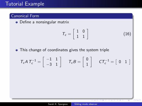
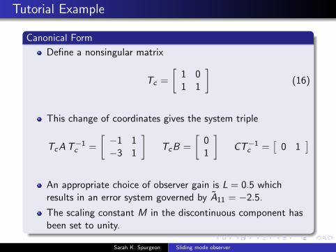
Canonical Form
Define a nonsingular matrix
Tc =
[1 01 1
](16)
This change of coordinates gives the system triple
TcAT−1c =
[−1 1−3 1
]TcB =
[01
]CT−1c =
[0 1
]An appropriate choice of observer gain is L = 0.5 whichresults in an error system governed by A11 = −2.5.
The scaling constant M in the discontinuous component hasbeen set to unity.
Sarah K. Spurgeon Sliding mode observer
Tutorial Example
Canonical Form
Define a nonsingular matrix
Tc =
[1 01 1
](16)
This change of coordinates gives the system triple
TcAT−1c =
[−1 1−3 1
]TcB =
[01
]CT−1c =
[0 1
]
An appropriate choice of observer gain is L = 0.5 whichresults in an error system governed by A11 = −2.5.
The scaling constant M in the discontinuous component hasbeen set to unity.
Sarah K. Spurgeon Sliding mode observer

Tutorial Example
Canonical Form
Define a nonsingular matrix
Tc =
[1 01 1
](16)
This change of coordinates gives the system triple
TcAT−1c =
[−1 1−3 1
]TcB =
[01
]CT−1c =
[0 1
]An appropriate choice of observer gain is L = 0.5 whichresults in an error system governed by A11 = −2.5.
The scaling constant M in the discontinuous component hasbeen set to unity.
Sarah K. Spurgeon Sliding mode observer
Tutorial Example
Canonical Form
Define a nonsingular matrix
Tc =
[1 01 1
](16)
This change of coordinates gives the system triple
TcAT−1c =
[−1 1−3 1
]TcB =
[01
]CT−1c =
[0 1
]An appropriate choice of observer gain is L = 0.5 whichresults in an error system governed by A11 = −2.5.
The scaling constant M in the discontinuous component hasbeen set to unity.
Sarah K. Spurgeon Sliding mode observer

Tutorial Example
The Figure shows the state estimation errors e1(t) and ey (t)resulting from the initial conditions e1 = −1 and ey = 0.Although the error system starts on the sliding surface So , anideal sliding motion cannot be maintained; only afterapproximately 1.2 seconds is sliding established.At this point in the time interval 1.2 to 3.0 seconds, e1(t)exhibits a first-order exponential decay to the origin.After 3.0 seconds almost perfect replication of the states takesplace.
-1
-0.5
0
0.5
1
0 1 2 3 4 5 6 7 8 9 10
Time, sec
Stat
e E
stim
atio
n E
rror
s
Figure : A sliding mode
Sarah K. Spurgeon Sliding mode observer
Tutorial Example
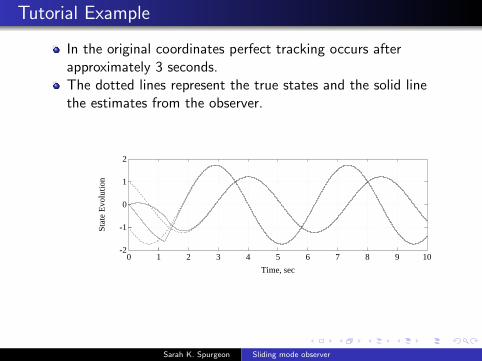
In the original coordinates perfect tracking occurs afterapproximately 3 seconds.The dotted lines represent the true states and the solid linethe estimates from the observer.
-2
-1
0
1
2
0 1 2 3 4 5 6 7 8 9 10
Time, sec
Stat
e E
volu
tion
Figure : A sliding mode
Sarah K. Spurgeon Sliding mode observer
Tutorial Example
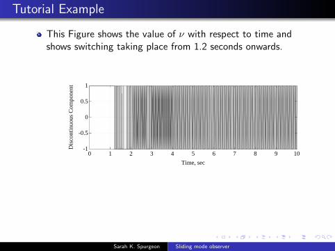
This Figure shows the value of ν with respect to time andshows switching taking place from 1.2 seconds onwards.
-1
-0.5
0
0.5
1
0 1 2 3 4 5 6 7 8 9 10
Time, sec
Dis
cont
inuo
us C
ompo
nent
Figure : A sliding mode
Sarah K. Spurgeon Sliding mode observer
Classical Utkin Observer with Linear Injection
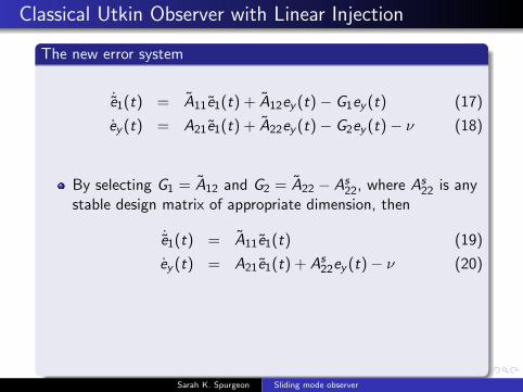
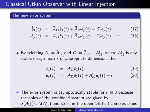
The new error system
˙e1(t) = A11e1(t) + A12ey (t)− G1ey (t) (17)
ey (t) = A21e1(t) + A22ey (t)− G2ey (t)− ν (18)
By selecting G1 = A12 and G2 = A22 − As22, where As
22 is anystable design matrix of appropriate dimension, then
˙e1(t) = A11e1(t) (19)
ey (t) = A21e1(t) + As22ey (t)− ν (20)
The error system is asymptotically stable for ν ≡ 0 becausethe poles of the combined system are given byλ(A11)∪ λ(As
22) and so lie in the open left half complex plane.
Sarah K. Spurgeon Sliding mode observer
Classical Utkin Observer with Linear Injection
The new error system
˙e1(t) = A11e1(t) + A12ey (t)− G1ey (t) (17)
ey (t) = A21e1(t) + A22ey (t)− G2ey (t)− ν (18)
By selecting G1 = A12 and G2 = A22 − As22, where As
22 is anystable design matrix of appropriate dimension, then
˙e1(t) = A11e1(t) (19)
ey (t) = A21e1(t) + As22ey (t)− ν (20)
The error system is asymptotically stable for ν ≡ 0 becausethe poles of the combined system are given byλ(A11)∪ λ(As
22) and so lie in the open left half complex plane.
Sarah K. Spurgeon Sliding mode observer
Classical Observer
Observations
In the original Utkin observer, the switching action ν waspotentially required to make the error system stable.
Thus far the only restriction imposed on the nominal linearsystem is that the pair (A,C ) is observable.
Sarah K. Spurgeon Sliding mode observer
Classical Observer
Observations
In the original Utkin observer, the switching action ν waspotentially required to make the error system stable.
Thus far the only restriction imposed on the nominal linearsystem is that the pair (A,C ) is observable.
Sarah K. Spurgeon Sliding mode observer

Further Historical Developments
The Slotine Observer (1980s)
The output errors are fed back in both a linear and adiscontinuous manner for nonlinear systems in companionform with the objective of ensuring a ’sliding patch’, whichdefines the region in which it is possible for the dynamicalobserver system to exhibit sliding behaviour, is maximised.
Once only a subset of state information is known, the ability ofany system to attain and maintain sliding will be more limitedthan in the situation where full state information is available.
With the Slotine observer, the linear feedback elements are aLuenberger observer with the role of the magnitude of thediscontinuous element to enhance robustness.
It is shown that a larger discontinuous element can enhancerobustness but this can be at the expense of increasedsensitivity to measurement noise.
Sarah K. Spurgeon Sliding mode observer

Further Historical Developments
The Walcott and Zak Observer, (1980s)
This was instrumental in defining the structural conditions forexistence of sliding mode observers for linear systems and laidimportant foundations for subsequent contributions whichformulated constructive design methodologies and includeduncertainty.
It was key in showing the promise of the methodology forobserver design for nonlinear systems, where methodologiesfor relatively general nonlinear system representations wereconsidered
These ideas will be developed further in the next lecture.
Sarah K. Spurgeon Sliding mode observer

Sliding mode observers: towards a constructivedesign framework
Sarah K. Spurgeon
School of Engineering and Digital ArtsUniversity of Kent, UK
Spring School, Aussois, June 2015
Sarah K. Spurgeon Sliding mode observer

Outline of Presentation
Walcott and Zak Observer
Introduction to a constructive sliding mode observer designframework
Potential of the discontinuous injection signal - lecture 3
Sarah K. Spurgeon Sliding mode observer

Outline of Presentation
Walcott and Zak Observer
Introduction to a constructive sliding mode observer designframework
Potential of the discontinuous injection signal - lecture 3
Sarah K. Spurgeon Sliding mode observer

Outline of Presentation
Walcott and Zak Observer
Introduction to a constructive sliding mode observer designframework
Potential of the discontinuous injection signal - lecture 3
Sarah K. Spurgeon Sliding mode observer

Outline of Presentation
Walcott and Zak Observer
Introduction to a constructive sliding mode observer designframework
Potential of the discontinuous injection signal - lecture 3
Sarah K. Spurgeon Sliding mode observer
Recap
Thus far the only restriction imposed on the nominal linearsystem is that the pair (A,C ) is observable.
Uncertainty and robustness has not been considered.
Sarah K. Spurgeon Sliding mode observer
Walcott and Zak Observer
System Representation
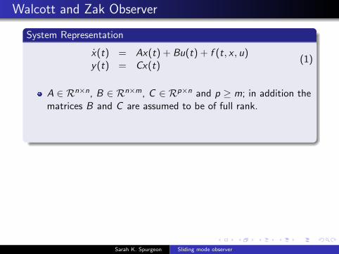
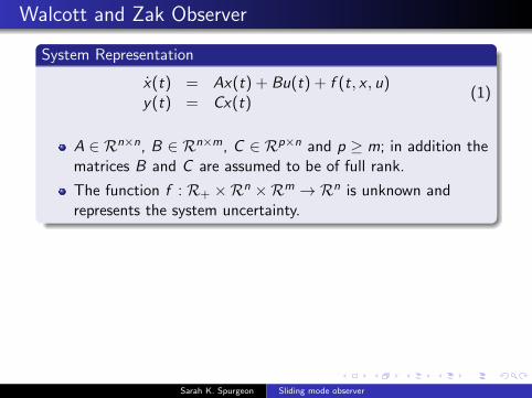
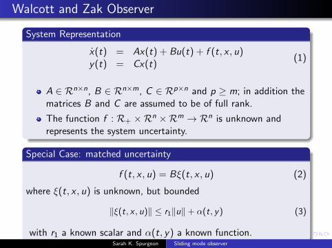
x(t) = Ax(t) + Bu(t) + f (t, x , u)y(t) = Cx(t)
(1)
A ∈ Rn×n, B ∈ Rn×m, C ∈ Rp×n and p ≥ m; in addition thematrices B and C are assumed to be of full rank.
The function f : R+ ×Rn ×Rm → Rn is unknown andrepresents the system uncertainty.
Special Case: matched uncertainty
f (t, x , u) = Bξ(t, x , u) (2)
where ξ(t, x , u) is unknown, but bounded
‖ξ(t, x , u)‖ ≤ r1‖u‖+ α(t, y) (3)
with r1 a known scalar and α(t, y) a known function.
Sarah K. Spurgeon Sliding mode observer
Walcott and Zak Observer
System Representation
x(t) = Ax(t) + Bu(t) + f (t, x , u)y(t) = Cx(t)
(1)
A ∈ Rn×n, B ∈ Rn×m, C ∈ Rp×n and p ≥ m; in addition thematrices B and C are assumed to be of full rank.
The function f : R+ ×Rn ×Rm → Rn is unknown andrepresents the system uncertainty.
Special Case: matched uncertainty
f (t, x , u) = Bξ(t, x , u) (2)
where ξ(t, x , u) is unknown, but bounded
‖ξ(t, x , u)‖ ≤ r1‖u‖+ α(t, y) (3)
with r1 a known scalar and α(t, y) a known function.Sarah K. Spurgeon Sliding mode observer
Walcott and Zak Observer
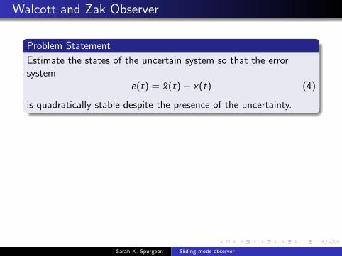
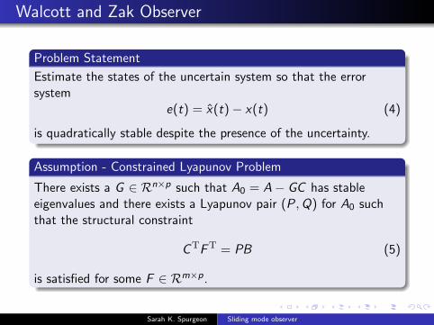
Problem Statement
Estimate the states of the uncertain system so that the errorsystem
e(t) = x(t)− x(t) (4)
is quadratically stable despite the presence of the uncertainty.
Assumption - Constrained Lyapunov Problem
There exists a G ∈ Rn×p such that A0 = A− GC has stableeigenvalues and there exists a Lyapunov pair (P,Q) for A0 suchthat the structural constraint
CTFT = PB (5)
is satisfied for some F ∈ Rm×p.
Sarah K. Spurgeon Sliding mode observer
Walcott and Zak Observer
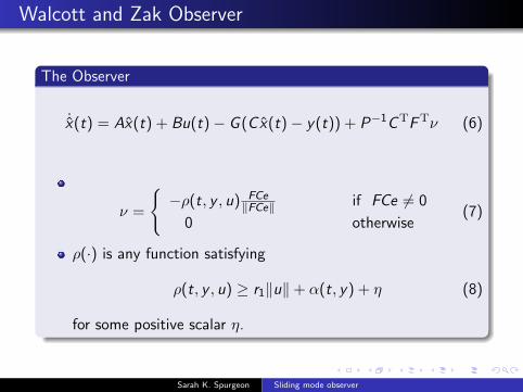
The Observer
˙x(t) = Ax(t) + Bu(t)− G (Cx(t)− y(t)) + P−1CTFTν (6)
ν =
−ρ(t, y , u) FCe
‖FCe‖ if FCe 6= 0
0 otherwise(7)
ρ(·) is any function satisfying
ρ(t, y , u) ≥ r1‖u‖+ α(t, y) + η (8)
for some positive scalar η.
Sarah K. Spurgeon Sliding mode observer

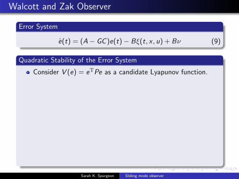
Walcott and Zak Observer
Error System
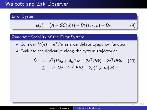
e(t) = (A− GC )e(t)− Bξ(t, x , u) + Bν (9)
Quadratic Stability of the Error System
Consider V (e) = eTPe as a candidate Lyapunov function.
Evaluate the derivative along the system trajectories
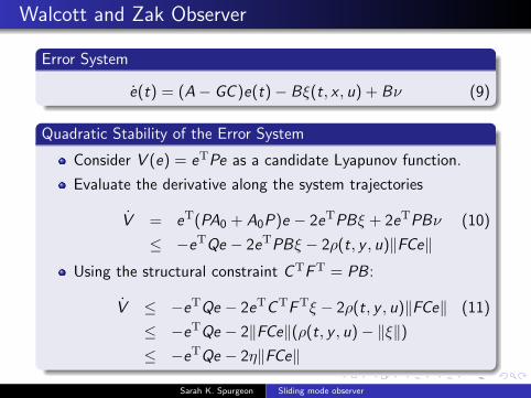
V = eT(PA0 + A0P)e − 2eTPBξ + 2eTPBν (10)
≤ −eTQe − 2eTPBξ − 2ρ(t, y , u)‖FCe‖Using the structural constraint CTFT = PB:
V ≤ −eTQe − 2eTCTFTξ − 2ρ(t, y , u)‖FCe‖ (11)
≤ −eTQe − 2‖FCe‖(ρ(t, y , u)− ‖ξ‖)≤ −eTQe − 2η‖FCe‖
Sarah K. Spurgeon Sliding mode observer
Walcott and Zak Observer
Error System
e(t) = (A− GC )e(t)− Bξ(t, x , u) + Bν (9)
Quadratic Stability of the Error System
Consider V (e) = eTPe as a candidate Lyapunov function.
Evaluate the derivative along the system trajectories
V = eT(PA0 + A0P)e − 2eTPBξ + 2eTPBν (10)
≤ −eTQe − 2eTPBξ − 2ρ(t, y , u)‖FCe‖
Using the structural constraint CTFT = PB:
V ≤ −eTQe − 2eTCTFTξ − 2ρ(t, y , u)‖FCe‖ (11)
≤ −eTQe − 2‖FCe‖(ρ(t, y , u)− ‖ξ‖)≤ −eTQe − 2η‖FCe‖
Sarah K. Spurgeon Sliding mode observer
Walcott and Zak Observer
Error System
e(t) = (A− GC )e(t)− Bξ(t, x , u) + Bν (9)
Quadratic Stability of the Error System
Consider V (e) = eTPe as a candidate Lyapunov function.
Evaluate the derivative along the system trajectories
V = eT(PA0 + A0P)e − 2eTPBξ + 2eTPBν (10)
≤ −eTQe − 2eTPBξ − 2ρ(t, y , u)‖FCe‖Using the structural constraint CTFT = PB:
V ≤ −eTQe − 2eTCTFTξ − 2ρ(t, y , u)‖FCe‖ (11)
≤ −eTQe − 2‖FCe‖(ρ(t, y , u)− ‖ξ‖)≤ −eTQe − 2η‖FCe‖
Sarah K. Spurgeon Sliding mode observer

Walcott and Zak Observer
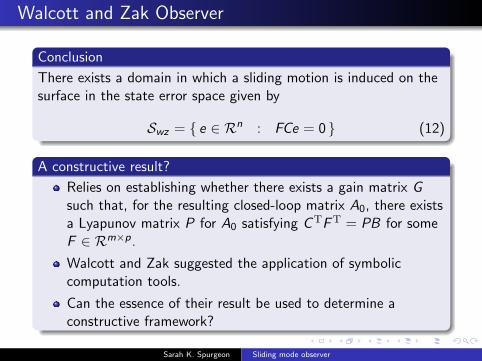
Conclusion
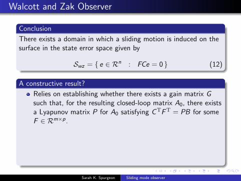
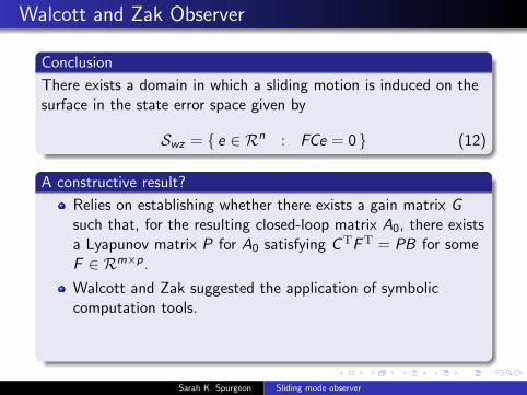
There exists a domain in which a sliding motion is induced on thesurface in the state error space given by
Swz = e ∈ Rn : FCe = 0 (12)
A constructive result?
Relies on establishing whether there exists a gain matrix Gsuch that, for the resulting closed-loop matrix A0, there existsa Lyapunov matrix P for A0 satisfying CTFT = PB for someF ∈ Rm×p.
Walcott and Zak suggested the application of symboliccomputation tools.
Can the essence of their result be used to determine aconstructive framework?
Sarah K. Spurgeon Sliding mode observer
Walcott and Zak Observer
Conclusion
There exists a domain in which a sliding motion is induced on thesurface in the state error space given by
Swz = e ∈ Rn : FCe = 0 (12)
A constructive result?
Relies on establishing whether there exists a gain matrix Gsuch that, for the resulting closed-loop matrix A0, there existsa Lyapunov matrix P for A0 satisfying CTFT = PB for someF ∈ Rm×p.
Walcott and Zak suggested the application of symboliccomputation tools.
Can the essence of their result be used to determine aconstructive framework?
Sarah K. Spurgeon Sliding mode observer
Sliding mode observers for linear uncertain systems
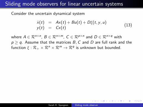
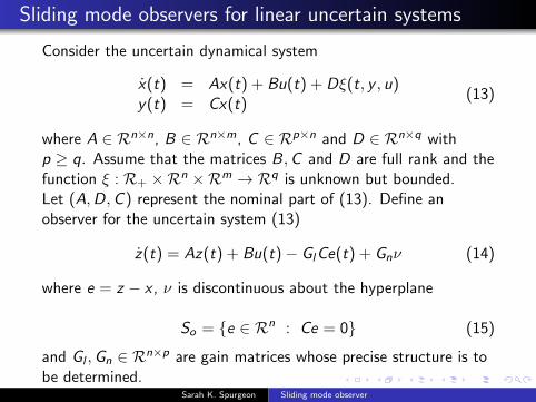
Consider the uncertain dynamical system
x(t) = Ax(t) + Bu(t) + Dξ(t, y , u)y(t) = Cx(t)
(13)
where A ∈ Rn×n, B ∈ Rn×m, C ∈ Rp×n and D ∈ Rn×q withp ≥ q. Assume that the matrices B,C and D are full rank and thefunction ξ : R+ ×Rn ×Rm → Rq is unknown but bounded.
Let (A,D,C ) represent the nominal part of (13). Define anobserver for the uncertain system (13)
z(t) = Az(t) + Bu(t)− GlCe(t) + Gnν (14)
where e = z − x , ν is discontinuous about the hyperplane
So = e ∈ Rn : Ce = 0 (15)
and Gl ,Gn ∈ Rn×p are gain matrices whose precise structure is tobe determined.
Sarah K. Spurgeon Sliding mode observer
Sliding mode observers for linear uncertain systems
Consider the uncertain dynamical system
x(t) = Ax(t) + Bu(t) + Dξ(t, y , u)y(t) = Cx(t)
(13)
where A ∈ Rn×n, B ∈ Rn×m, C ∈ Rp×n and D ∈ Rn×q withp ≥ q. Assume that the matrices B,C and D are full rank and thefunction ξ : R+ ×Rn ×Rm → Rq is unknown but bounded.Let (A,D,C ) represent the nominal part of (13). Define anobserver for the uncertain system (13)
z(t) = Az(t) + Bu(t)− GlCe(t) + Gnν (14)
where e = z − x , ν is discontinuous about the hyperplane
So = e ∈ Rn : Ce = 0 (15)
and Gl ,Gn ∈ Rn×p are gain matrices whose precise structure is tobe determined.
Sarah K. Spurgeon Sliding mode observer
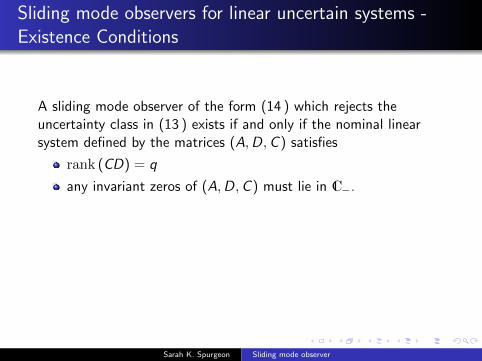
Sliding mode observers for linear uncertain systems -Existence Conditions
A sliding mode observer of the form (14 ) which rejects theuncertainty class in (13 ) exists if and only if the nominal linearsystem defined by the matrices (A,D,C ) satisfies
rank (CD) = q
any invariant zeros of (A,D,C ) must lie in C−.
For a square system the above two conditions require the triple(A,D,C ) to be relative degree one and minimum phase.These conditions depend upon a specific selection of uncertaintychannel and the observer design will be directly determined by theuncertainty distribution matrix.
Sarah K. Spurgeon Sliding mode observer
Sliding mode observers for linear uncertain systems -Existence Conditions
A sliding mode observer of the form (14 ) which rejects theuncertainty class in (13 ) exists if and only if the nominal linearsystem defined by the matrices (A,D,C ) satisfies
rank (CD) = q
any invariant zeros of (A,D,C ) must lie in C−.
For a square system the above two conditions require the triple(A,D,C ) to be relative degree one and minimum phase.
These conditions depend upon a specific selection of uncertaintychannel and the observer design will be directly determined by theuncertainty distribution matrix.
Sarah K. Spurgeon Sliding mode observer

Sliding mode observers for linear uncertain systems -Existence Conditions
A sliding mode observer of the form (14 ) which rejects theuncertainty class in (13 ) exists if and only if the nominal linearsystem defined by the matrices (A,D,C ) satisfies
rank (CD) = q
any invariant zeros of (A,D,C ) must lie in C−.
For a square system the above two conditions require the triple(A,D,C ) to be relative degree one and minimum phase.These conditions depend upon a specific selection of uncertaintychannel and the observer design will be directly determined by theuncertainty distribution matrix.
Sarah K. Spurgeon Sliding mode observer
Sliding mode observers for linear uncertain systems -Canonical Form for Design
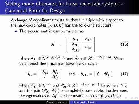
A change of coordinates exists so that the triple with respect tothe new coordinates (A, D, C ) has the following structure:
The system matrix can be written as
A =
A11 A12
A211
A212A22
(16)
where A11 ∈ R(n−p)×(n−p) and A211 ∈ R(p−q)×(n−p). Whenpartitioned these matrices have the structure
A11 =
[Ao11 Ao
12
0 Ao22
]and A211 =
[0 Ao
21
](17)
where Ao11 ∈ Rr×r and Ao
21 ∈ R(p−q)×(n−p−r) for some r ≥ 0and the pair (Ao
22,Ao21) is completely observable. Furthermore,
the eigenvalues of Ao11 are the invariant zeros of (A,D,C ).
Sarah K. Spurgeon Sliding mode observer

Sliding mode observers for linear uncertain systems -Canonical Form for Design
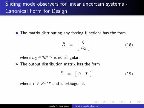
The matrix distributing any forcing functions has the form
D =
[0D2
](18)
where D2 ∈ Rq×q is nonsingular.
The output distribution matrix has the form
C =[
0 T]
(19)
where T ∈ Rp×p and is orthogonal.
Sarah K. Spurgeon Sliding mode observer
Sliding mode observers for linear uncertain systems -Canonical Form for Design
The matrix distributing any forcing functions has the form
D =
[0D2
](18)
where D2 ∈ Rq×q is nonsingular.
The output distribution matrix has the form
C =[
0 T]
(19)
where T ∈ Rp×p and is orthogonal.
Sarah K. Spurgeon Sliding mode observer

Sliding mode observers for linear uncertain systems -Canonical Form for Design
In order to ensure compatibility in the partition of the state-spacematrices, let
A21 =
[A211
A212
]and D =
[0D2
](20)
where D2 is defined as
D2 =
[0D2
]lp−qlq
(21)
The necessary and sufficient conditions for existence of a slidingmode observer together with the canonical form provide a pathwayto a constructive method for observer design.
Sarah K. Spurgeon Sliding mode observer

Sliding mode observers - a pathway to design
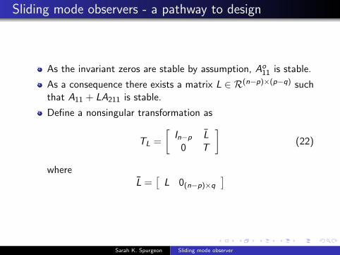
As the invariant zeros are stable by assumption, Ao11 is stable.
As a consequence there exists a matrix L ∈ R(n−p)×(p−q) suchthat A11 + LA211 is stable.
Define a nonsingular transformation as
TL =
[In−p L
0 T
](22)
whereL =
[L 0(n−p)×q
]
Sarah K. Spurgeon Sliding mode observer

Sliding mode observers - a pathway to design
As the invariant zeros are stable by assumption, Ao11 is stable.
As a consequence there exists a matrix L ∈ R(n−p)×(p−q) suchthat A11 + LA211 is stable.
Define a nonsingular transformation as
TL =
[In−p L
0 T
](22)
whereL =
[L 0(n−p)×q
]
Sarah K. Spurgeon Sliding mode observer
Sliding mode observers - a pathway to design
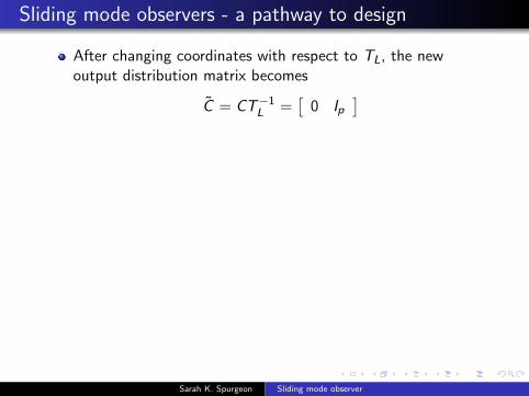
After changing coordinates with respect to TL, the newoutput distribution matrix becomes
C = CT−1L =[
0 Ip]
From the definition of L and D2
LD2 =[L 0
] [ 0D2
]= 0
and so the uncertainty distribution matrix is given by
D = TLD =
[LD2
TD2
]=
[0
TD2
]Finally, if A = TLAT−1L , it can be shown by direct evaluationthat
A11 = A11 + LA211
which is stable by choice of L.
Sarah K. Spurgeon Sliding mode observer
Sliding mode observers - a pathway to design
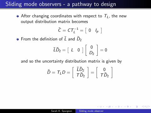
After changing coordinates with respect to TL, the newoutput distribution matrix becomes
C = CT−1L =[
0 Ip]
From the definition of L and D2
LD2 =[L 0
] [ 0D2
]= 0
and so the uncertainty distribution matrix is given by
D = TLD =
[LD2
TD2
]=
[0
TD2
]
Finally, if A = TLAT−1L , it can be shown by direct evaluationthat
A11 = A11 + LA211
which is stable by choice of L.
Sarah K. Spurgeon Sliding mode observer

Sliding mode observers - a pathway to design
After changing coordinates with respect to TL, the newoutput distribution matrix becomes
C = CT−1L =[
0 Ip]
From the definition of L and D2
LD2 =[L 0
] [ 0D2
]= 0
and so the uncertainty distribution matrix is given by
D = TLD =
[LD2
TD2
]=
[0
TD2
]Finally, if A = TLAT−1L , it can be shown by direct evaluationthat
A11 = A11 + LA211
which is stable by choice of L.
Sarah K. Spurgeon Sliding mode observer
Sliding mode observers - a pathway to design
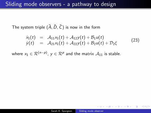
The system triple (A, D, C ) is now in the form
x1(t) = A11x1(t) +A12y(t) + B1u(t)y(t) = A21x1(t) +A22y(t) + B2u(t) +D2ξ
(23)
where x1 ∈ R(n−p), y ∈ Rp and the matrix A11 is stable.
Define the corresponding observer by
˙x1(t) = A11x1(t) +A12y(t) + B1u(t)−A12ey (t)˙y(t) = A21x1(t) +A22y(t) + B2u(t)− (A22 −As
22)ey (t) + ν
where As22 is a stable design matrix and ey = y − y .
Sarah K. Spurgeon Sliding mode observer

Sliding mode observers - a pathway to design
The system triple (A, D, C ) is now in the form
x1(t) = A11x1(t) +A12y(t) + B1u(t)y(t) = A21x1(t) +A22y(t) + B2u(t) +D2ξ
(23)
where x1 ∈ R(n−p), y ∈ Rp and the matrix A11 is stable.Define the corresponding observer by
˙x1(t) = A11x1(t) +A12y(t) + B1u(t)−A12ey (t)˙y(t) = A21x1(t) +A22y(t) + B2u(t)− (A22 −As
22)ey (t) + ν
where As22 is a stable design matrix and ey = y − y .
Sarah K. Spurgeon Sliding mode observer
Sliding mode observers - a pathway to design
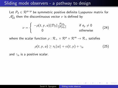
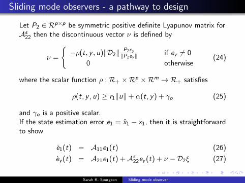
Let P2 ∈ Rp×p be symmetric positive definite Lyapunov matrix forAs
22 then the discontinuous vector ν is defined by
ν =
−ρ(t, y , u)‖D2‖ P2ey
‖P2ey‖ if ey 6= 0
0 otherwise(24)
where the scalar function ρ : R+ ×Rp ×Rm → R+ satisfies
ρ(t, y , u) ≥ r1‖u‖+ α(t, y) + γo (25)
and γo is a positive scalar.
If the state estimation error e1 = x1 − x1, then it is straightforwardto show
e1(t) = A11e1(t) (26)
ey (t) = A21e1(t) +As22ey (t) + ν −D2ξ (27)
Sarah K. Spurgeon Sliding mode observer
Sliding mode observers - a pathway to design
Let P2 ∈ Rp×p be symmetric positive definite Lyapunov matrix forAs
22 then the discontinuous vector ν is defined by
ν =
−ρ(t, y , u)‖D2‖ P2ey
‖P2ey‖ if ey 6= 0
0 otherwise(24)
where the scalar function ρ : R+ ×Rp ×Rm → R+ satisfies
ρ(t, y , u) ≥ r1‖u‖+ α(t, y) + γo (25)
and γo is a positive scalar.If the state estimation error e1 = x1 − x1, then it is straightforwardto show
e1(t) = A11e1(t) (26)
ey (t) = A21e1(t) +As22ey (t) + ν −D2ξ (27)
Sarah K. Spurgeon Sliding mode observer
Sliding mode observers - a pathway to design
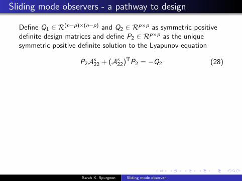
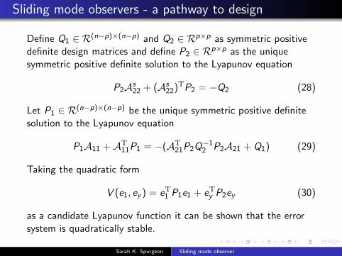
Define Q1 ∈ R(n−p)×(n−p) and Q2 ∈ Rp×p as symmetric positivedefinite design matrices and define P2 ∈ Rp×p as the uniquesymmetric positive definite solution to the Lyapunov equation
P2As22 + (As
22)TP2 = −Q2 (28)
Let P1 ∈ R(n−p)×(n−p) be the unique symmetric positive definitesolution to the Lyapunov equation
P1A11 +AT11P1 = −(AT
21P2Q−12 P2A21 + Q1) (29)
Taking the quadratic form
V (e1, ey ) = eT1 P1e1 + eTy P2ey (30)
as a candidate Lyapunov function it can be shown that the errorsystem is quadratically stable.
Sarah K. Spurgeon Sliding mode observer

Sliding mode observers - a pathway to design
Define Q1 ∈ R(n−p)×(n−p) and Q2 ∈ Rp×p as symmetric positivedefinite design matrices and define P2 ∈ Rp×p as the uniquesymmetric positive definite solution to the Lyapunov equation
P2As22 + (As
22)TP2 = −Q2 (28)
Let P1 ∈ R(n−p)×(n−p) be the unique symmetric positive definitesolution to the Lyapunov equation
P1A11 +AT11P1 = −(AT
21P2Q−12 P2A21 + Q1) (29)
Taking the quadratic form
V (e1, ey ) = eT1 P1e1 + eTy P2ey (30)
as a candidate Lyapunov function it can be shown that the errorsystem is quadratically stable.
Sarah K. Spurgeon Sliding mode observer

Sliding mode observers - a pathway to design
Further, consideration of the quadratic form
Vs(ey ) = eTy P2ey (31)
shows that an ideal sliding motion takes place on (15) and theoutput error ey enters Ω = (e1, ey ) : ‖A21e1‖ < ‖D2‖γo − ηwhere η is a small positive scalar in finite time and remains there.
Sarah K. Spurgeon Sliding mode observer
The Sliding Mode Observer
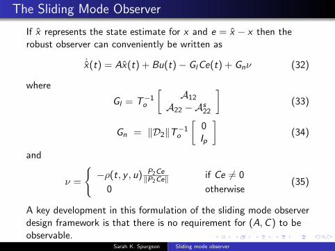
If x represents the state estimate for x and e = x − x then therobust observer can conveniently be written as
˙x(t) = Ax(t) + Bu(t)− GlCe(t) + Gnν (32)
where
Gl = T−1o
[A12
A22 −As22
](33)
Gn = ‖D2‖T−1o
[0Ip
](34)
and
ν =
−ρ(t, y , u) P2Ce
‖P2Ce‖ if Ce 6= 0
0 otherwise(35)
A key development in this formulation of the sliding mode observerdesign framework is that there is no requirement for (A,C ) to beobservable.
Sarah K. Spurgeon Sliding mode observer
Tutorial Example
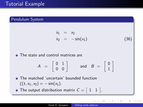
Pendulum System
x1 = x2
x2 = − sin(x1) (36)
The state and control matrices are
A =
[0 10 0
]and B =
[01
]The matched ‘uncertain’ bounded functionξ(t, x1, x2) = − sin(x1).
The output distribution matrix C =[
1 1].
Sarah K. Spurgeon Sliding mode observer
Tutorial Example
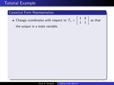
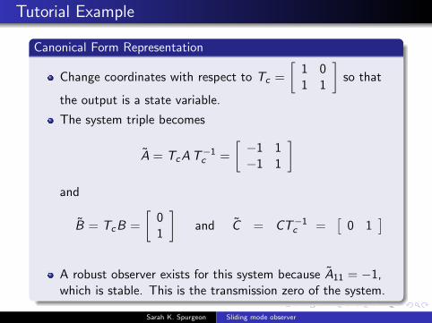
Canonical Form Representation
Change coordinates with respect to Tc =
[1 01 1
]so that
the output is a state variable.
The system triple becomes
A = TcAT−1c =
[−1 1−1 1
]and
B = TcB =
[01
]and C = CT−1c =
[0 1
]A robust observer exists for this system because A11 = −1,which is stable. This is the transmission zero of the system.
Sarah K. Spurgeon Sliding mode observer

Tutorial Example
Canonical Form Representation
Change coordinates with respect to Tc =
[1 01 1
]so that
the output is a state variable.
The system triple becomes
A = TcAT−1c =
[−1 1−1 1
]and
B = TcB =
[01
]and C = CT−1c =
[0 1
]
A robust observer exists for this system because A11 = −1,which is stable. This is the transmission zero of the system.
Sarah K. Spurgeon Sliding mode observer
Tutorial Example
Canonical Form Representation
Change coordinates with respect to Tc =
[1 01 1
]so that
the output is a state variable.
The system triple becomes
A = TcAT−1c =
[−1 1−1 1
]and
B = TcB =
[01
]and C = CT−1c =
[0 1
]A robust observer exists for this system because A11 = −1,which is stable. This is the transmission zero of the system.
Sarah K. Spurgeon Sliding mode observer

Tutorial Example
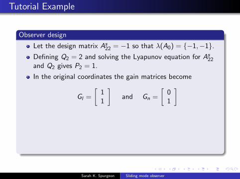
Observer design
Let the design matrix As22 = −1 so that λ(A0) = −1,−1.
Defining Q2 = 2 and solving the Lyapunov equation for As22
and Q2 gives P2 = 1.
In the original coordinates the gain matrices become
Gl =
[11
]and Gn =
[01
]
The observer becomes
d
dt
[x1x2
]=
[−1 0−1 −1
] [x1x2
]+
[11
]y +
[01
]ν
Sarah K. Spurgeon Sliding mode observer

Tutorial Example
Observer design
Let the design matrix As22 = −1 so that λ(A0) = −1,−1.
Defining Q2 = 2 and solving the Lyapunov equation for As22
and Q2 gives P2 = 1.
In the original coordinates the gain matrices become
Gl =
[11
]and Gn =
[01
]
The observer becomes
d
dt
[x1x2
]=
[−1 0−1 −1
] [x1x2
]+
[11
]y +
[01
]ν
Sarah K. Spurgeon Sliding mode observer
Tutorial Example
Observer design
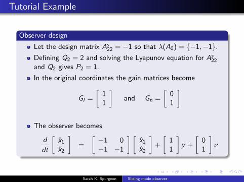
Let the design matrix As22 = −1 so that λ(A0) = −1,−1.
Defining Q2 = 2 and solving the Lyapunov equation for As22
and Q2 gives P2 = 1.
In the original coordinates the gain matrices become
Gl =
[11
]and Gn =
[01
]
The observer becomes
d
dt
[x1x2
]=
[−1 0−1 −1
] [x1x2
]+
[11
]y +
[01
]ν
Sarah K. Spurgeon Sliding mode observer

Tutorial Example
Demonstrates the nonlinear observer tracking the output fromthe pendulum when the initial conditions of the true statesand observer states are deliberately set to different values
-2
-1
0
1
2
0 2 4 6 8 10 12 14 16 18 20
Time, sec
Out
puts
Sarah K. Spurgeon Sliding mode observer

Tutorial Example
A comparison of the true and estimated states.After approximately 4 seconds, visually perfect replication ofthe states is taking place.
-2
-1
0
1
2
0 2 4 6 8 10 12 14 16 18 20
Time, sec
Firs
t Sta
te
-2
-1
0
1
2
0 2 4 6 8 10 12 14 16 18 20
Seco
nd S
tate
Time, secSarah K. Spurgeon Sliding mode observer
Tutorial Example
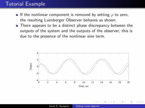
If the nonlinear component is removed by setting ρ to zero,the resulting Luenberger Observer behaves as shown.There appears to be a distinct phase discrepancy between theoutputs of the system and the outputs of the observer; this isdue to the presence of the nonlinear sine term.
-4
-2
0
2
4
0 2 4 6 8 10 12 14 16 18 20
Time, sec
Out
put
Sarah K. Spurgeon Sliding mode observer
Tutorial Example
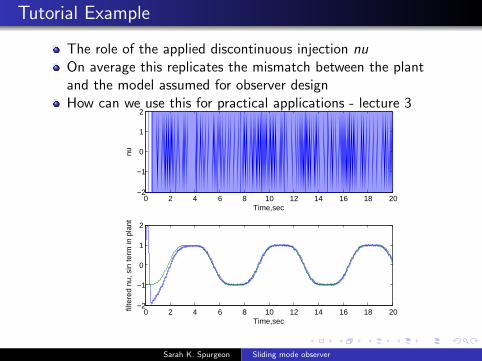
The role of the applied discontinuous injection nuOn average this replicates the mismatch between the plantand the model assumed for observer designHow can we use this for practical applications - lecture 3
0 2 4 6 8 10 12 14 16 18 20−2
−1
0
1
2
Time,sec
nu
0 2 4 6 8 10 12 14 16 18 20−2
−1
0
1
2
Time,sec
filte
red
nu, s
in te
rm in
pla
nt
Sarah K. Spurgeon Sliding mode observer

Sliding mode observers: a robust conditionmonitoring and fault detection tool
Sarah K. Spurgeon
School of Engineering and Digital ArtsUniversity of Kent, UK
Spring School, Aussois, June 2015
Sarah K. Spurgeon Sliding mode observer

Sliding Mode Observers
Outline of Presentation
Principle of the equivalent injection - Fault detection andisolation
Fault detection and isolation - a case study
A sampled framework for practical application? - lecture 4
Sarah K. Spurgeon Sliding mode observer
Sliding Mode Observers
Outline of Presentation
Principle of the equivalent injection - Fault detection andisolation
Fault detection and isolation - a case study
A sampled framework for practical application? - lecture 4
Sarah K. Spurgeon Sliding mode observer
Sliding Mode Observers
Outline of Presentation
Principle of the equivalent injection - Fault detection andisolation
Fault detection and isolation - a case study
A sampled framework for practical application? - lecture 4
Sarah K. Spurgeon Sliding mode observer
Sliding Mode Observers
Outline of Presentation
Principle of the equivalent injection - Fault detection andisolation
Fault detection and isolation - a case study
A sampled framework for practical application? - lecture 4
Sarah K. Spurgeon Sliding mode observer

Sliding Mode Observers
Recap
We have developed constructive frameworks for design
We have noted in the tutorial example that when an observerdesigned based on the dynamics of the double integrator isapplied to a nonlinear pendulum system, the discontinuoussignal when in the sliding mode, on average, reconstructs themismatch between the model used for design and the plantused for implementation
Sarah K. Spurgeon Sliding mode observer

Sliding mode observers for fault detection and faultreconstruction
Historical Perspective
One of the first papers designed an observer so that theobserver error moves from the switching surface and slidingceases in the presence of a fault.
This approach is difficult to implement in practice - the choiceof gain to maintain sliding motion from the theory is oftenconservative and therefore it is difficult to ensure a faultinduces a break in sliding.
Observers, when exhibiting sliding motion, enable faultsand/or values of immeasurable system parameters to bereconstructed using the principle of the equivalent injectionsignal.
Sarah K. Spurgeon Sliding mode observer

Sliding mode observers for fault detection and faultreconstruction
Nominal linear system subject to input/actuator and sensor faults
x(t) = Ax(t) + Bu(t) + Dfi (t) (1)
y(t) = Cx(t) + fo(t) (2)
A ∈ Rn×n, B ∈ Rn×m, C ∈ Rp×n, D ∈ Rn×q with q ≤ p < nand the matrices B,C and D are of full rank.
The function fi (t) represents an actuator fault.
fo(t) represents and sensor faults
It is assumed that the states of the system are unknown andonly the signals u(t) and y(t) are available.
Sarah K. Spurgeon Sliding mode observer
The Observer
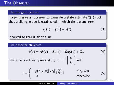
The design objective
To synthesise an observer to generate a state estimate x(t) suchthat a sliding mode is established in which the output error
ey (t) = y(t)− y(t) (3)
is forced to zero in finite time.
The observer structure
˙x(t) = Ax(t) + Bu(t)− Gley (t) + Gnν (4)
where Gl is a linear gain and Gn = T−1o
[0Ip
]with
ν =
−ρ(t, y , u)‖D2‖ P2ey
‖P2ey‖ if ey 6= 0
0 otherwise(5)
Sarah K. Spurgeon Sliding mode observer
The Observer
The design objective
To synthesise an observer to generate a state estimate x(t) suchthat a sliding mode is established in which the output error
ey (t) = y(t)− y(t) (3)
is forced to zero in finite time.
The observer structure
˙x(t) = Ax(t) + Bu(t)− Gley (t) + Gnν (4)
where Gl is a linear gain and Gn = T−1o
[0Ip
]with
ν =
−ρ(t, y , u)‖D2‖ P2ey
‖P2ey‖ if ey 6= 0
0 otherwise(5)
Sarah K. Spurgeon Sliding mode observer
The Error Dynamics
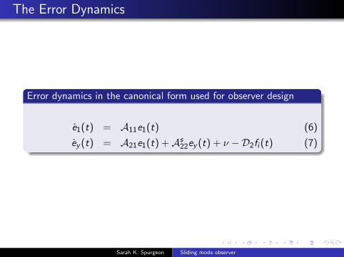
Error dynamics in the canonical form used for observer design
e1(t) = A11e1(t) (6)
ey (t) = A21e1(t) +As22ey (t) + ν −D2fi (t) (7)
Sarah K. Spurgeon Sliding mode observer
Fault Reconstruction
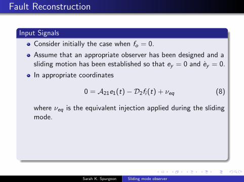
Input Signals
Consider initially the case when fo = 0.
Assume that an appropriate observer has been designed and asliding motion has been established so that ey = 0 and ey = 0.
In appropriate coordinates
0 = A21e1(t)−D2fi (t) + νeq (8)
where νeq is the equivalent injection applied during the slidingmode.
From the stability of the e1 subsystem, it follows thate1(t)→ 0 and therefore
νeq → D2fi (t) (9)
Sarah K. Spurgeon Sliding mode observer

Fault Reconstruction
Input Signals
Consider initially the case when fo = 0.
Assume that an appropriate observer has been designed and asliding motion has been established so that ey = 0 and ey = 0.
In appropriate coordinates
0 = A21e1(t)−D2fi (t) + νeq (8)
where νeq is the equivalent injection applied during the slidingmode.
From the stability of the e1 subsystem, it follows thate1(t)→ 0 and therefore
νeq → D2fi (t) (9)
Sarah K. Spurgeon Sliding mode observer
Fault Reconstruction
Input Signals
A commonly used approach to reconstruct the equivalentinjection is to use a low pass filter. Alternatively replace thediscontinuous injection by the continuous approximation
νδ = −ρ‖D2‖ P2ey‖P2ey‖+δ (10)
where δ is a small positive scalar.
The equivalent control can be approximated by (10) to anyrequired accuracy by a small enough choice of δ. Sincerank(D2) = q it follows that
fi (t) ≈ −ρ‖D2‖(DT2 D2)−1DT
2P2ey (t)
‖P2ey (t)‖+δ (11)
The equivalent injection signal can be computed on-line anddepends only on the output estimation error ey ; thus the faultfi can be approximated to any degree of accuracy.
Sarah K. Spurgeon Sliding mode observer
Detection of faults at the output
Methodology
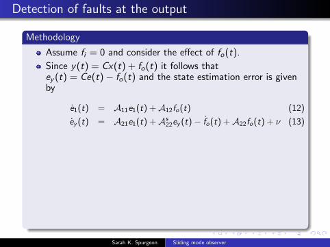
Assume fi = 0 and consider the effect of fo(t).
Since y(t) = Cx(t) + fo(t) it follows thatey (t) = Ce(t)− fo(t) and the state estimation error is givenby
e1(t) = A11e1(t) +A12fo(t) (12)
ey (t) = A21e1(t) +As22ey (t)− fo(t) +A22fo(t) + ν (13)
fo(t) and fo(t) are output disturbances; ρ must be chosensufficiently large to maintain sliding
During sliding 0 = A21e1 − fo(t) +A22fo(t) + νeq and forslowly varying faults
νeq ≈ −(A22 −A21A−111 A12)fo (14)
Sarah K. Spurgeon Sliding mode observer
Detection of faults at the output
Methodology
Assume fi = 0 and consider the effect of fo(t).
Since y(t) = Cx(t) + fo(t) it follows thatey (t) = Ce(t)− fo(t) and the state estimation error is givenby
e1(t) = A11e1(t) +A12fo(t) (12)
ey (t) = A21e1(t) +As22ey (t)− fo(t) +A22fo(t) + ν (13)
fo(t) and fo(t) are output disturbances; ρ must be chosensufficiently large to maintain sliding
During sliding 0 = A21e1 − fo(t) +A22fo(t) + νeq and forslowly varying faults
νeq ≈ −(A22 −A21A−111 A12)fo (14)
Sarah K. Spurgeon Sliding mode observer
Output fault detection
Methodology
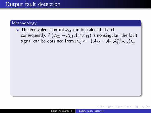
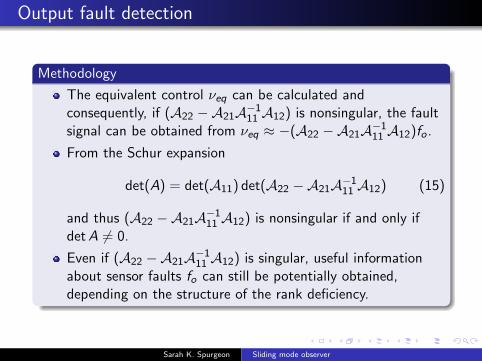
The equivalent control νeq can be calculated andconsequently, if (A22 −A21A−111 A12) is nonsingular, the faultsignal can be obtained from νeq ≈ −(A22 −A21A−111 A12)fo .
From the Schur expansion
det(A) = det(A11) det(A22 −A21A−111 A12) (15)
and thus (A22 −A21A−111 A12) is nonsingular if and only ifdet A 6= 0.
Even if (A22 −A21A−111 A12) is singular, useful informationabout sensor faults fo can still be potentially obtained,depending on the structure of the rank deficiency.
Sarah K. Spurgeon Sliding mode observer

Output fault detection
Methodology
The equivalent control νeq can be calculated andconsequently, if (A22 −A21A−111 A12) is nonsingular, the faultsignal can be obtained from νeq ≈ −(A22 −A21A−111 A12)fo .
From the Schur expansion
det(A) = det(A11) det(A22 −A21A−111 A12) (15)
and thus (A22 −A21A−111 A12) is nonsingular if and only ifdet A 6= 0.
Even if (A22 −A21A−111 A12) is singular, useful informationabout sensor faults fo can still be potentially obtained,depending on the structure of the rank deficiency.
Sarah K. Spurgeon Sliding mode observer
Example: Inverted Pendulum with a Cart
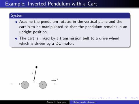
System
Assume the pendulum rotates in the vertical plane and thecart is to be manipulated so that the pendulum remains in anupright position.
The cart is linked by a transmission belt to a drive wheelwhich is driven by a DC motor.
θ
x
Sarah K. Spurgeon Sliding mode observer
Example: Inverted Pendulum with a Cart
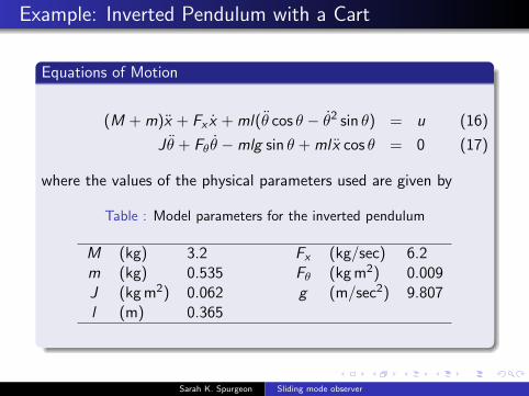
Equations of Motion
(M + m)x + Fx x + ml(θ cos θ − θ2 sin θ) = u (16)
J θ + Fθθ −mlg sin θ + mlx cos θ = 0 (17)
where the values of the physical parameters used are given by
Table : Model parameters for the inverted pendulum
M (kg) 3.2 Fx (kg/sec) 6.2m (kg) 0.535 Fθ (kg m2) 0.009J (kg m2) 0.062 g (m/sec2) 9.807l (m) 0.365
Sarah K. Spurgeon Sliding mode observer
Linear model
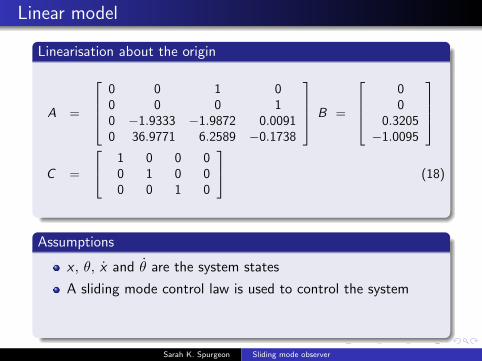
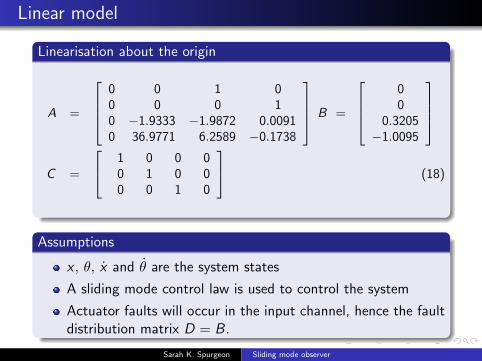
Linearisation about the origin
A =
0 0 1 00 0 0 10 −1.9333 −1.9872 0.00910 36.9771 6.2589 −0.1738
B =
00
0.3205−1.0095
C =
1 0 0 00 1 0 00 0 1 0
(18)
Assumptions
x , θ, x and θ are the system states
A sliding mode control law is used to control the system
Actuator faults will occur in the input channel, hence the faultdistribution matrix D = B.
Sarah K. Spurgeon Sliding mode observer
Linear model
Linearisation about the origin
A =
0 0 1 00 0 0 10 −1.9333 −1.9872 0.00910 36.9771 6.2589 −0.1738
B =
00
0.3205−1.0095
C =
1 0 0 00 1 0 00 0 1 0
(18)
Assumptions
x , θ, x and θ are the system states
A sliding mode control law is used to control the system
Actuator faults will occur in the input channel, hence the faultdistribution matrix D = B.
Sarah K. Spurgeon Sliding mode observer
Numerical methods for design
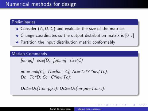
Preliminaries
Consider (A,D,C ) and evaluate the size of the matrices
Change coordinates so the output distribution matrix is [0 I ]
Partition the input distribution matrix conformably
Matlab Commands
[nn,qq]=size(D); [pp,nn]=size(C)
nc = null(C); Tc=[nc’; C]; Ac=Tc*A*inv(Tc);Dc=Tc*D; Cc=C*inv(Tc);
Dc1=Dc(1:nn-pp,:); Dc2=Dc(nn-pp+1:nn,:);
Sarah K. Spurgeon Sliding mode observer
Numerical methods for design
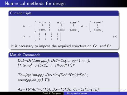
Current triple
Ac =
−0.1738 0 36.9771 6.2589
0 0 0 11 0 0 0
0.0091 0 −1.9333 −1.9872
Bc =
−0.0095
00
0.3205
Cc =
0 1 0 00 0 1 00 0 0 1
(19)
It is necessary to impose the required structure on Cc and Bc
Matlab Commands
Dc1=Dc(1:nn-pp,:); Dc2=Dc(nn-pp+1:nn,:);[T,temp]=qr(Dc2); T=(flipud(T’))’;
Tb=[eye(nn-pp) -Dc1*inv(Dc2’*Dc2)*Dc2’;zeros(pp,nn-pp) T’];
Aa=Tb*Ac*inv(Tb); Da=Tb*Dc; Ca=Cc*inv(Tb);Sarah K. Spurgeon Sliding mode observer

Numerical Methods for Design
Current Triple
Aa =
−0.1451 0 30.8877 −0.4568
0 0 0 11 0 0 3.1498
−0.0091 0 1.9333 −2.0159
Ba =
0
00
−0.3205
Ca =
0 − 1 0 00 0 1 00 0 0 −1
(20)
The system has no transmission zeros and thus the transformationto separate the unobservable modes is not requiredDetermine a gain matrix so that the top left sub-system has thedesired poles
Matlab Commands
tzero(Aa,Da,Ca,zeros(pp,qq))A22o=Aa(1:nn-pp,1:nn-pp);A21o=Aa(nn-pp+1:nn-qq,1:nn-pp);L=place(A22o’,A21o’,-10)’;
Sarah K. Spurgeon Sliding mode observer
Numerical Methods for Design
Matlab Commands
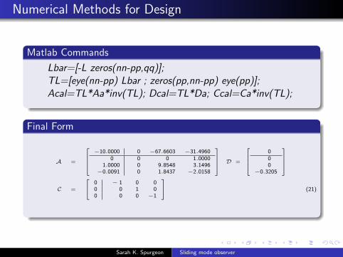
Lbar=[-L zeros(nn-pp,qq)];TL=[eye(nn-pp) Lbar ; zeros(pp,nn-pp) eye(pp)];Acal=TL*Aa*inv(TL); Dcal=TL*Da; Ccal=Ca*inv(TL);
Final Form
A =
−10.0000 0 −67.6603 −31.4960
0 0 0 1.00001.0000 0 9.8548 3.1496−0.0091 0 1.8437 −2.0158
D =
000
−0.3205
C =
0 − 1 0 00 0 1 00 0 0 −1
(21)
Sarah K. Spurgeon Sliding mode observer
Recap: Sliding mode observers - a pathway to design
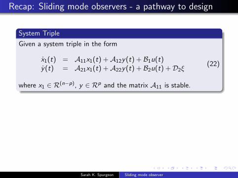
System Triple
Given a system triple in the form
x1(t) = A11x1(t) +A12y(t) + B1u(t)y(t) = A21x1(t) +A22y(t) + B2u(t) +D2ξ
(22)
where x1 ∈ R(n−p), y ∈ Rp and the matrix A11 is stable.
Corresponding Observer
˙x1(t) = A11x1(t) +A12y(t) + B1u(t)−A12ey (t)˙y(t) = A21x1(t) +A22y(t) + B2u(t)− (A22 −As
22)ey (t) + ν
where As22 is a stable design matrix and ey = y − y .
Sarah K. Spurgeon Sliding mode observer

Recap: Sliding mode observers - a pathway to design
System Triple
Given a system triple in the form
x1(t) = A11x1(t) +A12y(t) + B1u(t)y(t) = A21x1(t) +A22y(t) + B2u(t) +D2ξ
(22)
where x1 ∈ R(n−p), y ∈ Rp and the matrix A11 is stable.
Corresponding Observer
˙x1(t) = A11x1(t) +A12y(t) + B1u(t)−A12ey (t)˙y(t) = A21x1(t) +A22y(t) + B2u(t)− (A22 −As
22)ey (t) + ν
where As22 is a stable design matrix and ey = y − y .
Sarah K. Spurgeon Sliding mode observer

Example: Inverted Pendulum with a Cart
Canonical Form Representation
A =
−10.0000 0 −67.6603 −31.4960
0 0 0 1.00001.0000 0 9.8548 3.1496−0.0091 0 1.8437 −2.0158
D =
000
−0.3205
C =
0 − 1 0 00 0 1 00 0 0 −1
(23)
Observer Design
By design A11 = −10
As22 = diag(−11,−12,−13) - the linear component of the
observer poles are approximately three times faster than theclosed-loop poles of the controlled plant.
The symmetric positive definite matrix P2 satisfiesP2A22 +AT
22P2 = −I
The scalar function ρ = 75Sarah K. Spurgeon Sliding mode observer
Nonlinear simulation testing
Fault Reconstruction
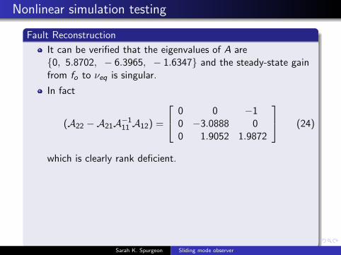
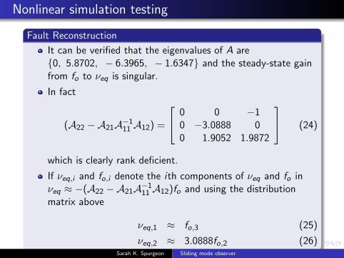
It can be verified that the eigenvalues of A are0, 5.8702, − 6.3965, − 1.6347 and the steady-state gainfrom fo to νeq is singular.
In fact
(A22 −A21A−111 A12) =
0 0 −10 −3.0888 00 1.9052 1.9872
(24)
which is clearly rank deficient.
If νeq,i and fo,i denote the ith components of νeq and fo inνeq ≈ −(A22 −A21A−111 A12)fo and using the distributionmatrix above
νeq,1 ≈ fo,3 (25)
νeq,2 ≈ 3.0888fo,2 (26)
Sarah K. Spurgeon Sliding mode observer
Nonlinear simulation testing
Fault Reconstruction
It can be verified that the eigenvalues of A are0, 5.8702, − 6.3965, − 1.6347 and the steady-state gainfrom fo to νeq is singular.
In fact
(A22 −A21A−111 A12) =
0 0 −10 −3.0888 00 1.9052 1.9872
(24)
which is clearly rank deficient.
If νeq,i and fo,i denote the ith components of νeq and fo inνeq ≈ −(A22 −A21A−111 A12)fo and using the distributionmatrix above
νeq,1 ≈ fo,3 (25)
νeq,2 ≈ 3.0888fo,2 (26)Sarah K. Spurgeon Sliding mode observer

Nonlinear simulation testing
Fault Reconstruction
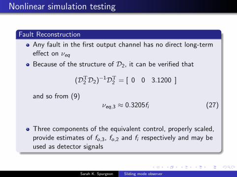
Any fault in the first output channel has no direct long-termeffect on νeq
Because of the structure of D2, it can be verified that
(DT2 D2)−1DT
2 = [ 0 0 3.1200 ]
and so from (9)νeq,3 ≈ 0.3205fi (27)
Three components of the equivalent control, properly scaled,provide estimates of fo,3, fo,2 and fi respectively and may beused as detector signals
Sarah K. Spurgeon Sliding mode observer
Nonlinear simulation testing
Fault Reconstruction
Any fault in the first output channel has no direct long-termeffect on νeq
Because of the structure of D2, it can be verified that
(DT2 D2)−1DT
2 = [ 0 0 3.1200 ]
and so from (9)νeq,3 ≈ 0.3205fi (27)
Three components of the equivalent control, properly scaled,provide estimates of fo,3, fo,2 and fi respectively and may beused as detector signals
Sarah K. Spurgeon Sliding mode observer
Nonlinear simulation testing
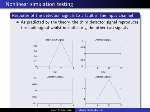
Response of the detection signals to a fault in the input channel
As predicted by the theory, the third detector signal reproducesthe fault signal whilst not affecting the other two signals
0
0.2
0.4
0.6
0.8
1
0 5 10 15
Input Fault Signal
Time
-0.1
-0.05
0
0.05
0.1
0 5 10 15
Detector Signal 1
Time
-0.1
-0.05
0
0.05
0.1
0 5 10 15
Detector Signal 2
Time
0
0.5
1
0 5 10 15
Detector Signal 3
TimeSarah K. Spurgeon Sliding mode observer
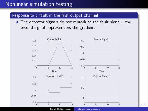
Nonlinear simulation testing
Response to a fault in the first output channel
The detector signals do not reproduce the fault signal - thesecond signal approximates the gradient
0
0.02
0.04
0.06
0.08
0.1
0 5 10 15
Output Fault 1
Time
-0.1
-0.05
0
0.05
0.1
0 5 10 15
Detctor Signal 1
Time
-0.1
-0.05
0
0.05
0.1
0 5 10 15
Detector Signal 2
Time
0
0.5
1
0 5 10 15
Detector Signal 3
TimeSarah K. Spurgeon Sliding mode observer
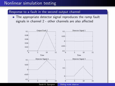
Nonlinear simulation testing
Response to a fault in the second output channel
The appropriate detector signal reproduces the ramp faultsignals in channel 2 - other channels are also affected
0
0.02
0.04
0.06
0.08
0.1
0 5 10 15
Output Fault 2
Time
-0.1
-0.05
0
0.05
0.1
0 5 10 15
Detector Signal 1
Time
-0.1
-0.05
0
0.05
0.1
0 5 10 15
Detector Signal 2
Time
0
0.5
1
0 5 10 15
Detector Signal 3
TimeSarah K. Spurgeon Sliding mode observer

Nonlinear simulation testing
Response to a fault in the third output channel
The appropriate detector signal reproduces the ramp faultsignals in channel 3 - other channels are also affected
0
0.02
0.04
0.06
0.08
0.1
0 5 10 15
Output Fault 3
Time
-0.1
-0.05
0
0.05
0.1
0 5 10 15
Detector Signal 1
Time
-0.1
-0.05
0
0.05
0.1
0 5 10 15
Detector Signal 2
Time
0
0.5
1
0 5 10 15
Detector Signal 3
TimeSarah K. Spurgeon Sliding mode observer
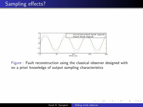
Sampling effects?
0 5 10 15 20−2
−1
0
1
2
time (s)
reconstructed fault signalinput fault signal
Figure : Fault reconstruction using the classical observer designed withno a priori knowledge of output sampling characteristics
Sarah K. Spurgeon Sliding mode observer

Concluding remarks
Fault detection and isolation (FDI) using sliding mode observers
The principle of the equivalent injection is a strong result tounder pin the development of FDI schemes
Constructive design approach and can run in real time
There is a conflict between theory and practice in that processmeasurements may be sampled at a rate which is notquasi-continuous and the sampling can impact on the fidelityof the reconstruction
Sarah K. Spurgeon Sliding mode observer

Sliding mode observers: implementation as acondition monitoring tool
Sarah K. Spurgeon
School of Engineering and Digital ArtsUniversity of Kent, UK
Spring School, Aussois, June 2015
Sarah K. Spurgeon Sliding mode observer

Sliding Mode Observers
Outline of Presentation
Parameter Estimation - an industrial case study
A sampled framework for the design of sliding mode observers
Sarah K. Spurgeon Sliding mode observer
Sliding Mode Observers
Outline of Presentation
Parameter Estimation - an industrial case study
A sampled framework for the design of sliding mode observers
Sarah K. Spurgeon Sliding mode observer

Sliding Mode Observers
Outline of Presentation
Parameter Estimation - an industrial case study
A sampled framework for the design of sliding mode observers
Sarah K. Spurgeon Sliding mode observer

Sliding Mode Observers
Recap
We have developed constructive frameworks for observerdesign
We have seen that sliding mode observers are a natural toolfor the development of FDI schemes
We have also seen via an example that sampling of the signalsused to drive the observer can affect the fidelity of thereconstruction
Sarah K. Spurgeon Sliding mode observer
Fault detection via parameter monitoring - An Example
A sliding mode observer can be used to estimate or monitorthe variation in system parameters.
The development and implementation of a simple conditionmonitoring system for a high speed rotating machine will beconsidered.As such machines become more complex and valuable, there isa greater need to protect them, and the systems they support,from the consequences of breakdown. This is relevant in thesemiconductor industry, for example, where machine failurecan cause the loss of a valuable batch of wafers.Dry vacuum pumps have been successfully used in thesemiconductor industry but the harsh nature of manysemiconductor processes creates a challenge for conditionmonitoring. Any diagnostic scheme should be able to operateunder all conditions and be able to detect faults, creating analarm to warn the user that maintenance must beconveniently scheduled before catastrophic loss occurs.
Sarah K. Spurgeon Sliding mode observer
Fault detection via parameter monitoring - An Example
A sliding mode observer can be used to estimate or monitorthe variation in system parameters.The development and implementation of a simple conditionmonitoring system for a high speed rotating machine will beconsidered.
As such machines become more complex and valuable, there isa greater need to protect them, and the systems they support,from the consequences of breakdown. This is relevant in thesemiconductor industry, for example, where machine failurecan cause the loss of a valuable batch of wafers.Dry vacuum pumps have been successfully used in thesemiconductor industry but the harsh nature of manysemiconductor processes creates a challenge for conditionmonitoring. Any diagnostic scheme should be able to operateunder all conditions and be able to detect faults, creating analarm to warn the user that maintenance must beconveniently scheduled before catastrophic loss occurs.
Sarah K. Spurgeon Sliding mode observer

Fault detection via parameter monitoring - An Example
A sliding mode observer can be used to estimate or monitorthe variation in system parameters.The development and implementation of a simple conditionmonitoring system for a high speed rotating machine will beconsidered.As such machines become more complex and valuable, there isa greater need to protect them, and the systems they support,from the consequences of breakdown. This is relevant in thesemiconductor industry, for example, where machine failurecan cause the loss of a valuable batch of wafers.
Dry vacuum pumps have been successfully used in thesemiconductor industry but the harsh nature of manysemiconductor processes creates a challenge for conditionmonitoring. Any diagnostic scheme should be able to operateunder all conditions and be able to detect faults, creating analarm to warn the user that maintenance must beconveniently scheduled before catastrophic loss occurs.
Sarah K. Spurgeon Sliding mode observer
Fault detection via parameter monitoring - An Example
A sliding mode observer can be used to estimate or monitorthe variation in system parameters.The development and implementation of a simple conditionmonitoring system for a high speed rotating machine will beconsidered.As such machines become more complex and valuable, there isa greater need to protect them, and the systems they support,from the consequences of breakdown. This is relevant in thesemiconductor industry, for example, where machine failurecan cause the loss of a valuable batch of wafers.Dry vacuum pumps have been successfully used in thesemiconductor industry but the harsh nature of manysemiconductor processes creates a challenge for conditionmonitoring. Any diagnostic scheme should be able to operateunder all conditions and be able to detect faults, creating analarm to warn the user that maintenance must beconveniently scheduled before catastrophic loss occurs.
Sarah K. Spurgeon Sliding mode observer

Consider a model for monitoring cooling water flow in a dryvacuum pump in the absence of a flow transducer. Heat transferthrough the system is illustrated below:
Electrical Power Dry Vacuum Pump
Convection to
atmosphere
Coolant inlet Coolant
outlet
Figure : A schematic of heat transfer in the dry vacuum pump
Sarah K. Spurgeon Sliding mode observer
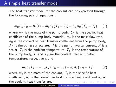
A simple heat transfer model
The heat transfer model for the coolant can be expressed throughthe following pair of equations.
mBCB TB = KI (t)− mcCc (To − Ti )− hBAB (TB − Ta) (1)
where mB is the mass of the pump body, CB is the specific heatcoefficient of the pump body material, mc is the mass flow rate,hB is the convective heat transfer coefficient from the pump body,AB is the pump surface area, I is the pump inverter current, K is ascalar, Ta is the ambient temperature, TB is the temperature ofthe pump body, Ti and To are the coolant inlet and outlettemperatures respectively, and
mcCc To = −mcCc (TB − To) + hcAc (TB − To) (2)
where mc is the mass of the coolant, Cc is the specific heatcoefficient, hc is the convective heat transfer coefficient and Ac isthe coolant heat transfer area.
Sarah K. Spurgeon Sliding mode observer
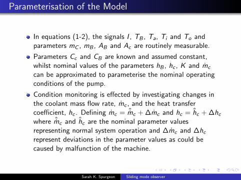
Parameterisation of the Model
In equations (1-2), the signals I , TB , Ta, Ti and To andparameters mC , mB , AB and Ac are routinely measurable.
Parameters Cc and CB are known and assumed constant,whilst nominal values of the parameters hB , hc , K and mc
can be approximated to parameterise the nominal operatingconditions of the pump.
Condition monitoring is effected by investigating changes inthe coolant mass flow rate, mc , and the heat transfercoefficient, hc . Defining mc = ˆmc + ∆mc and hc = hc + ∆hc
where ˆmc and hc are the nominal parameter valuesrepresenting normal system operation and ∆mc and ∆hc
represent deviations in the parameter values as could becaused by malfunction of the machine.
Sarah K. Spurgeon Sliding mode observer
Sliding mode observer
Define a pair of sliding mode observers by
mBCBˆTB = KI (t)− ˆmcCc (To − Ti )− hBAB
(TB − Ta
)− β1eb + νb
mcCcˆTo = − ˆmcCc
(TB − To
)+ hcAc (TB − To)− β2eo + νo
where
ei = Ti − Ti
nui = Kiei‖ei‖
(3)
for i = o,B where β1, β2,Ki > 0.The parameters β1, β2 provide asymptotic error decay and thediscontinuous terms nui ensure a sliding mode is attained onei = 0 so that the output error signals between the observer andthe measurement are kept identically at zero.
Sarah K. Spurgeon Sliding mode observer
Sliding mode analysis
Forming the error dynamics and noting that the sliding modecondition yields ei = ei = 0, it follows that
0 = ∆ ˆmcCc (To − Ti )− νb0 = ∆ ˆmcCc
(TB − To
)−∆hcAc (TB − To)− νo
The applied observer injection signals can be readily used tomonitor deviations in the nominal parameters.Note that this is a unique property of sliding mode observers thatcan only be realised by application of a discontinuous injectionsignal. Other observer formulations would not attain and maintainan identically zero output error but would seek to minimise theerror. This latter paradigm is not useful for parameterreconstruction.
Sarah K. Spurgeon Sliding mode observer

Observer performance under the start-up phase of normaloperation of the dry vacuum pump
Figure : Observer performance under nominal operation of the dryvacuum pump
Sarah K. Spurgeon Sliding mode observer
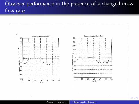
Observer performance in the presence of a changed massflow rate
Figure : Observer performance in the presence of a changed mass flowrate
A valve is used to reduce the mass of coolant flowing into thesystem at approximately 3200 seconds, and the correspondingchange in mass flow rate as predicted by the sliding mode observersystem
Sarah K. Spurgeon Sliding mode observer
Fault reconstruction under output sampling - a time delayapproach
A sliding mode observer in the presence of sampled outputinformation and its application to fault reconstruction isstudied.
The observer is designed by using the delayed continuous-timerepresentation of the sampled-data system, for which a set ofLinear Matrix Inequalities (LMIs) provide conditions for theultimate boundedness, where the bound is proportional to thesampling time and the magnitude of the switching gain.
It is shown that, for a sufficiently small value of µ, aperturbation parameter, a transducer or sensor fault can bereconstructed reliably from the output error dynamics.
Sarah K. Spurgeon Sliding mode observer
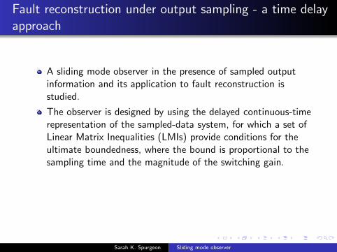

Problem Formulation
Consider the linear, time-invariant system with sampledoutputs
x(t) = Ax(t) + Bu(t) + Dfi (t)y(t) = Cxd(tk), tk ≤ t < tk+1
(4)
where x ∈ Rn, u ∈ Rm are the state and the input vectorrespectively and y ∈ Rp is a discrete-time outputmeasurement generated by zero-order hold functions with asequence of hold times 0 = t0 < t1 · · · < tk < · · · , wherelimk→∞ tk =∞.
fi ∈ Rq represents an unknown actuator fault which isassumed to be bounded by ‖fi (t)‖ ≤ ∆.
It is assumed q ≤ p < n and A, B, C , D are constantmatrices of appropriate dimensions.
Sarah K. Spurgeon Sliding mode observer
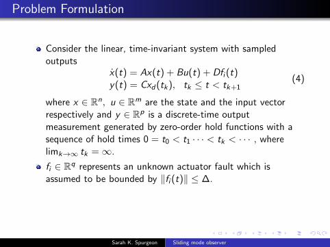
Problem Formulation
Consider the linear, time-invariant system with sampledoutputs
x(t) = Ax(t) + Bu(t) + Dfi (t)y(t) = Cxd(tk), tk ≤ t < tk+1
(4)
where x ∈ Rn, u ∈ Rm are the state and the input vectorrespectively and y ∈ Rp is a discrete-time outputmeasurement generated by zero-order hold functions with asequence of hold times 0 = t0 < t1 · · · < tk < · · · , wherelimk→∞ tk =∞.
fi ∈ Rq represents an unknown actuator fault which isassumed to be bounded by ‖fi (t)‖ ≤ ∆.
It is assumed q ≤ p < n and A, B, C , D are constantmatrices of appropriate dimensions.
Sarah K. Spurgeon Sliding mode observer
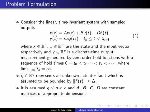
Problem Formulation
Consider the linear, time-invariant system with sampledoutputs
x(t) = Ax(t) + Bu(t) + Dfi (t)y(t) = Cxd(tk), tk ≤ t < tk+1
(4)
where x ∈ Rn, u ∈ Rm are the state and the input vectorrespectively and y ∈ Rp is a discrete-time outputmeasurement generated by zero-order hold functions with asequence of hold times 0 = t0 < t1 · · · < tk < · · · , wherelimk→∞ tk =∞.
fi ∈ Rq represents an unknown actuator fault which isassumed to be bounded by ‖fi (t)‖ ≤ ∆.
It is assumed q ≤ p < n and A, B, C , D are constantmatrices of appropriate dimensions.
Sarah K. Spurgeon Sliding mode observer
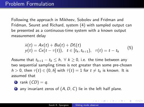
Problem Formulation
Following the approach in Mikheev, Sobolev and Fridman andFridman, Seuret and Richard, system (4) with sampled output canbe presented as a continuous-time system with a known outputmeasurement delay
x(t) = Ax(t) + Bu(t) + Dfi (t)y(t) = Cx(t − τ(t)), t ∈ [tk , tk+1), τ(t) = t − tk
(5)
Assume that tk+1 − tk ≤ h, ∀ k ≥ 0, i.e. the time between anytwo sequential sampling times is not greater than some pre-chosenh > 0, then τ(t) ∈ (0, h] with τ(t) = 1 for t 6= tk is known. It isassumed that
1 rank (CD) = q.
2 any invariant zeros of (A,D,C ) lie in the left half plane.
Sarah K. Spurgeon Sliding mode observer
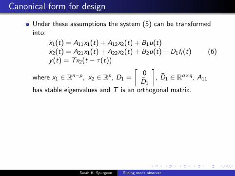
Canonical form for design
Under these assumptions the system (5) can be transformedinto:
x1(t) = A11x1(t) + A12x2(t) + B1u(t)x2(t) = A21x1(t) + A22x2(t) + B2u(t) + D1fi (t)y(t) = Tx2(t − τ(t))
(6)
where x1 ∈ Rn−p, x2 ∈ Rp, D1 =
[0
D1
], D1 ∈ Rq×q, A11
has stable eigenvalues and T is an orthogonal matrix.
An observer will be designed which, for sufficiently large t,induces motion in the h∆-neighbourhood of the surface
E = x2, x2 ∈ Rp : se(t) = T(x2(t−τ(t))−x2(t−τ(t))
)= 0
(7)where x2(t − τ(t)) is the corresponding component of theestimated states from an observer.An ideal sliding mode can be achieved with h = 0 underassumptions 1, 2.
Sarah K. Spurgeon Sliding mode observer
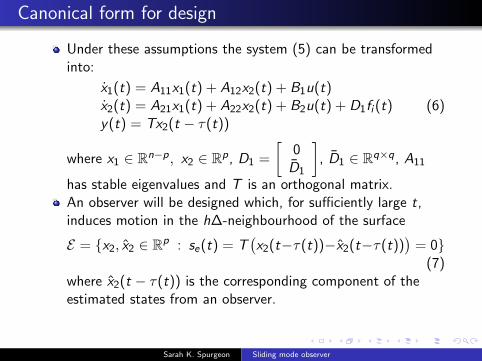
Canonical form for design
Under these assumptions the system (5) can be transformedinto:
x1(t) = A11x1(t) + A12x2(t) + B1u(t)x2(t) = A21x1(t) + A22x2(t) + B2u(t) + D1fi (t)y(t) = Tx2(t − τ(t))
(6)
where x1 ∈ Rn−p, x2 ∈ Rp, D1 =
[0
D1
], D1 ∈ Rq×q, A11
has stable eigenvalues and T is an orthogonal matrix.An observer will be designed which, for sufficiently large t,induces motion in the h∆-neighbourhood of the surface
E = x2, x2 ∈ Rp : se(t) = T(x2(t−τ(t))−x2(t−τ(t))
)= 0
(7)where x2(t − τ(t)) is the corresponding component of theestimated states from an observer.
An ideal sliding mode can be achieved with h = 0 underassumptions 1, 2.
Sarah K. Spurgeon Sliding mode observer

Canonical form for design
Under these assumptions the system (5) can be transformedinto:
x1(t) = A11x1(t) + A12x2(t) + B1u(t)x2(t) = A21x1(t) + A22x2(t) + B2u(t) + D1fi (t)y(t) = Tx2(t − τ(t))
(6)
where x1 ∈ Rn−p, x2 ∈ Rp, D1 =
[0
D1
], D1 ∈ Rq×q, A11
has stable eigenvalues and T is an orthogonal matrix.An observer will be designed which, for sufficiently large t,induces motion in the h∆-neighbourhood of the surface
E = x2, x2 ∈ Rp : se(t) = T(x2(t−τ(t))−x2(t−τ(t))
)= 0
(7)where x2(t − τ(t)) is the corresponding component of theestimated states from an observer.An ideal sliding mode can be achieved with h = 0 underassumptions 1, 2.
Sarah K. Spurgeon Sliding mode observer
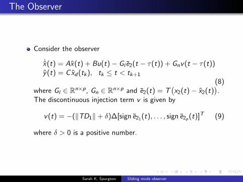
The Observer
Consider the observer
˙x(t) = Ax(t) + Bu(t)− Gl e2(t − τ(t)) + Gnv(t − τ(t))y(t) = C xd(tk), tk ≤ t < tk+1
(8)where Gl ∈ Rn×p, Gn ∈ Rn×p and e2(t) = T
(x2(t)− x2(t)
).
The discontinuous injection term v is given by
v(t) = −(‖TD1‖+ δ)∆[sign e21(t), . . . , sign e2p(t)]T (9)
where δ > 0 is a positive number.
Sarah K. Spurgeon Sliding mode observer
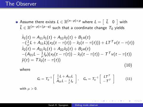
The Observer
Assume there exists L ∈ R(n−p)×p where L =[
L 0]
with
L ∈ R(n−p)×(p−q) such that a coordinate change T0 yields
˙x1(t) = A11x1(t) + A12x2(t) + B1u(t)−( 1
µL + A11L)(x2(t − τ(t))− x2(t − τ(t))) + LTT v(t − τ(t))˙x2(t) = A21x1(t) + A22x2(t) + B2u(t)−(A21L− 1
µ Ip)(x2(t − τ(t))− x2(t − τ(t))− TT v(t − τ(t))
y(t) = T x2(t − τ(t))(10)
where
Gl = T−10
[ 1µL + A11L
A21L− 1µIp
], Gn = T−1
0
[LTT
−TT
](11)
with µ > 0.
Sarah K. Spurgeon Sliding mode observer

The error dynamics
Defining the state estimation error as e1(t) = x1(t)− x1(t) ande2(t) = x2(t)− x2(t), and performing a change of coordinates such
that
[e1(t)e2(t)
]= TL
[e1(t)e2(t)
]with TL =
[In−q L
0 T
]. Since
LD1 = 0, one obtains
˙e1(t) = (A11 + LA21)e1(t)− (A11L + LA21L− A12
−LA22)TT e2(t) + (A11 + LA21)e2(t − τ(t))(12)
˙e2(t) = TA21e1(t)− (TA21LTT − TA22TT )e2(t)+TA21LTT e2(t − τ(t))− 1
µ e2(t − τ(t))
+v(t − τ(t)) + TD1fi (t)
(13)
with initial condition
e(t0) = e0, e(t) = 0, t < t0 (14)
Sarah K. Spurgeon Sliding mode observer
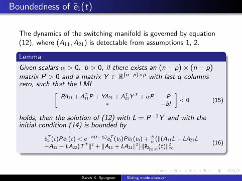
Boundedness of e1(t)
The dynamics of the switching manifold is governed by equation(12), where (A11,A21) is detectable from assumptions 1, 2.
Lemma
Given scalars α > 0, b > 0, if there exists an (n − p)× (n − p)matrix P > 0 and a matrix Y ∈ R(n−p)×p with last q columnszero, such that the LMI[
PA11 + AT11P + YA21 + AT
21YT + αP −P
∗ −bI
]< 0 (15)
holds, then the solution of (12) with L = P−1Y and with theinitial condition (14) is bounded by
eT1 (t)Pe1(t) < e−α(t−t0)eT1 (t0)Pe1(t0) + bα
(‖(A11L + LA21L
−A12 − LA22)TT‖2 + ‖A11 + LA21‖2)‖e2[t0,t]
(t)‖2∞
(16)
Sarah K. Spurgeon Sliding mode observer
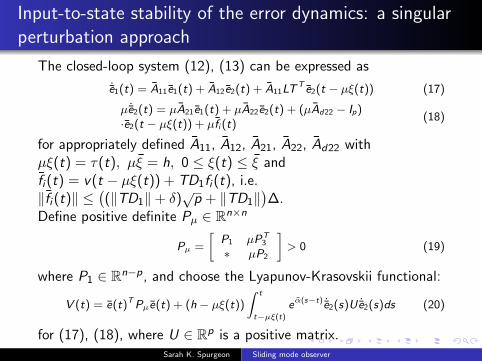
Input-to-state stability of the error dynamics: a singularperturbation approach
The closed-loop system (12), (13) can be expressed as
˙e1(t) = A11e1(t) + A12e2(t) + A11LTT e2(t − µξ(t)) (17)
µ ˙e2(t) = µA21e1(t) + µA22e2(t) + (µAd22 − Ip)·e2(t − µξ(t)) + µfi (t)
(18)
for appropriately defined A11, A12, A21, A22, Ad22 withµξ(t) = τ(t), µξ = h, 0 ≤ ξ(t) ≤ ξ andfi (t) = v(t − µξ(t)) + TD1fi (t), i.e.‖fi (t)‖ ≤
((‖TD1‖+ δ)
√p + ‖TD1‖
)∆.
Define positive definite Pµ ∈ Rn×n
Pµ =
[P1 µPT
3
∗ µP2
]> 0 (19)
where P1 ∈ Rn−p, and choose the Lyapunov-Krasovskii functional:
V (t) = e(t)TPµe(t) + (h − µξ(t))
∫ t
t−µξ(t)
eα(s−t) ˙e2(s)U ˙e2(s)ds (20)
for (17), (18), where U ∈ Rp is a positive matrix.Sarah K. Spurgeon Sliding mode observer
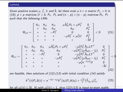
Lemma
Given positive scalars µ, ξ, α and b, let there exist a n × n matrix Pµ > 0 in(19), p × p matrices U > 0, P4, P5 and (n − p)× (n − p) matrices P6, P7
such that the following LMIs
Θµ0 =
θ11 θ12 θ13
∗ θ22 θ23
∗ ∗ −PT7
∗ ∗ ∗∗ ∗ ∗
µAT21P5 + µPT
3 0θ24 PT
4
0 0−µPT
5 + µξU PT5
∗ −bI
< 0 (21)
Θµ1 =
θ11 θ12 θ13 µAT21P5 + µPT
3 −µξPT6 A11LT
T 0∗ θ22 θ23 θ24 −µξPT
4 (µAd22 − Ip) PT4
∗ ∗ −PT7 0 −µξPT
7 A11LTT 0
∗ ∗ ∗ −µPT5 −µξPT
5 (µAd22 − Ip) PT5
∗ ∗ ∗ ∗ −µξe−αµξU 0∗ ∗ ∗ ∗ ∗ −bI
< 0
(22)are feasible, then solutions of (12)-(13) with initial condition (14) satisfy
eT (t)Pµe(t) < e−α(t−t0)eT (t0)Pµe(t0) + µ2 bα‖fi [t0,t]‖2
∞ (23)
for all µξ(t) ∈ [0, h] with µξ(t) = 1, thus (12)-(13) is input-to-state stable.Sarah K. Spurgeon Sliding mode observer
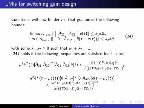
LMIs for switching gain design
Conditions will now be derived that guarantee the followingbounds:
lim supt→∞ ‖[
A21 A22
]e(t)‖ ≤ k1δ∆,
lim supt→∞ ‖[
0 Ad22
]e(t − τ(t))‖ ≤ k2δ∆
(24)
with some k1, k2 ≥ 0 such that k1 + k2 = 1.(24) holds if the following inequalities are satisfied for t →∞:
µ2eT (t)[A21 A22]T [A21 A22]e(t) <αeT (t)Pµe(t)k2
1 δ2
b(
(‖TD1‖+δ)√p+‖TD1‖
)2
µ2eT (t − µξ(t))[0 Ad22]T [0 Ad22]e(t − µξ(t))
<αeT (t−µξ(t))Pµe(t−µξ(t))k2
2 δ2
b(
(‖TD1‖+δ)√p+‖TD1‖
)2
Sarah K. Spurgeon Sliding mode observer

LMIs for switching gain design
Hence, the inequalities −k21 M1P1 −µk2
1 M1PT3 µAT
21
∗ −µk21 M1P2 µAT
22
∗ ∗ −Ip
< 0 −k22 M1P1 −µk2
2 M1PT3 0
∗ −µk22 M1P2 µAT
d22
∗ ∗ −Ip
< 0
(25)
where M1 = αδ2
b(
(‖TD1‖+δ)√p+‖TD1‖
)2 , guarantee that the solutions
of (12), (13) satisfy the bound (24).
Sarah K. Spurgeon Sliding mode observer

Ultimate boundedness of the error dynamics
Theorem
Given positive constants µ, ξ, α, b and k1, k2, let there exist an × n-matrix Pµ > 0, positive p × p-matrices U > 0 and p × pmatrices P4, P5, (n − p)× (n − p) matrices P6, P7 such thatLMIs (19), (21), (22) and (25) are feasible. Let e(t) be a solutionto (12), (13), then every component of e2(t) satisfies the bound
lim supt→∞
|e2i (t)| ≤ 2M0µξ (26)
where M0 = 2(δ + ‖TD1‖)∆, i = 1, . . . , p denotes the i-thcomponent of e2 for all µξ(t) ∈ [0, h] with µξ(t) = 1.
Sarah K. Spurgeon Sliding mode observer
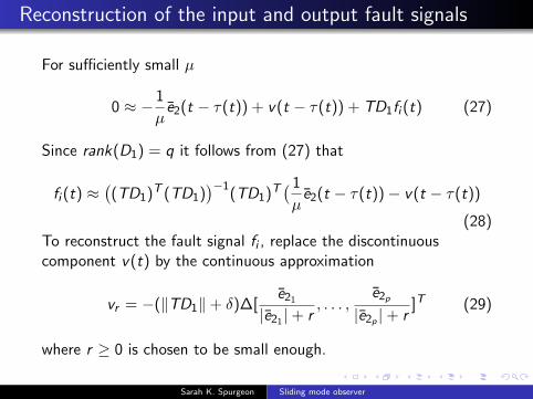
Reconstruction of the input and output fault signals
For sufficiently small µ
0 ≈ − 1
µe2(t − τ(t)) + v(t − τ(t)) + TD1fi (t) (27)
Since rank(D1) = q it follows from (27) that
fi (t) ≈((TD1)T (TD1)
)−1(TD1)T
( 1
µe2(t − τ(t))− v(t − τ(t))
(28)To reconstruct the fault signal fi , replace the discontinuouscomponent v(t) by the continuous approximation
vr = −(‖TD1‖+ δ)∆[e21
|e21 |+ r, . . . ,
e2p
|e2p |+ r]T (29)
where r ≥ 0 is chosen to be small enough.
Sarah K. Spurgeon Sliding mode observer

Reconstruction of the input and output fault signals
Now consider the case when fi = 0 and consider the effect of afault f0(t) at the output. In this situation, x2 is replaced byx2 → x2 + f0 and ey = e2 + f0. For sufficiently small µ, it can beobtained that
e1(t) ≈ −A−111 ( L
µ + A11L)f0
ey (t) = A21e1(t) + A22ey (t)− A22f0
+(A21L− Ipµ )ey (t − τ(t)) + TT v(t − τ(t)) + f0
(30)
The fault can be approximated by
f0 ≈W−1((A22L− Ip
µ )ey (t − τ(t)) + TT v(t − τ(t)))
(31)
if W = A21A−111 ( L
µ + A11L) + A22 is invertible.
Sarah K. Spurgeon Sliding mode observer
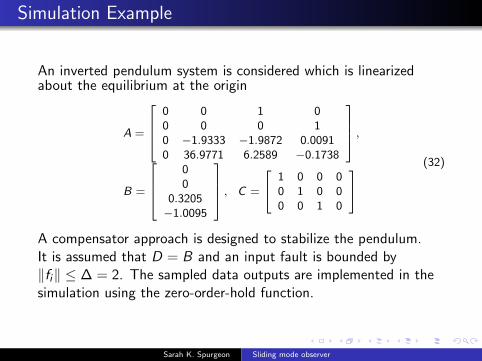
Simulation Example
An inverted pendulum system is considered which is linearizedabout the equilibrium at the origin
A =
0 0 1 00 0 0 10 −1.9333 −1.9872 0.00910 36.9771 6.2589 −0.1738
,
B =
00
0.3205−1.0095
, C =
1 0 0 00 1 0 00 0 1 0
(32)
A compensator approach is designed to stabilize the pendulum.It is assumed that D = B and an input fault is bounded by‖fi‖ ≤ ∆ = 2. The sampled data outputs are implemented in thesimulation using the zero-order-hold function.
Sarah K. Spurgeon Sliding mode observer
Example continued
In the LMI (15), L = [0 1.526 0] is obtained. LMIs (21) and (22)are feasible with α = 8, µ = 0.019, ξ = 0.524, i.e. the samplingperiod is given by µξ = 0.01s. LMI (25) is feasible with δ = 77and k1 = 0.8, k2 = 0.2. Hence the observer (8) with gains in (11)and (9) has been chosen which ensures the error variable isbounded in the range |e2i (t)| ≤ 6.2 according to the estimate (26).
Sarah K. Spurgeon Sliding mode observer
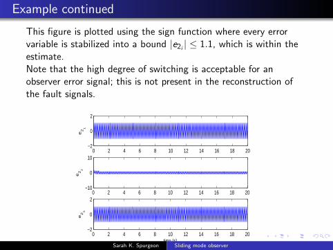
Example continued
This figure is plotted using the sign function where every errorvariable is stabilized into a bound |e2i | ≤ 1.1, which is within theestimate.Note that the high degree of switching is acceptable for anobserver error signal; this is not present in the reconstruction ofthe fault signals.
0 2 4 6 8 10 12 14 16 18 20−2
0
2
e2
1
0 2 4 6 8 10 12 14 16 18 20−10
0
10
e2
2
0 2 4 6 8 10 12 14 16 18 20−2
0
2
time (s)
e2
3
Figure : Error response e2 with sampling period h = 0.01s at outputs.
Sarah K. Spurgeon Sliding mode observer
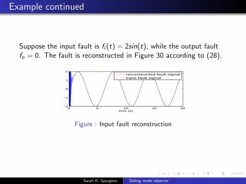
Example continued
Suppose the input fault is fi (t) = 2sin(t), while the output faultfo = 0. The fault is reconstructed in Figure 30 according to (28).
0 5 10 15 20−2
−1
0
1
2
time (s)
reconstructed fault signalinput fault signal
Figure : Input fault reconstruction
Sarah K. Spurgeon Sliding mode observer

Example continued
From the fault distribution structure
W =
0 0 10 −4.77 −3.150 −1.97 −2.01
only the third output fault can be reconstructed. This can beapproximated as the equivalent injection signal at the firstchannel of (A22L− Ip
µ )ey (t − τ(t)) + TT v(t − τ(t)).
Suppose the third output fault f03 = 5sin(t), the fault signal isreconstructed accurately under the sampled output withsampling period h = 0.01s.
0 5 10 15 20−5
0
5
time (s)
reconstructed fault signaloutput fault signal
Figure : Output fault reconstruction in the third component of theoutput vector
Sarah K. Spurgeon Sliding mode observer
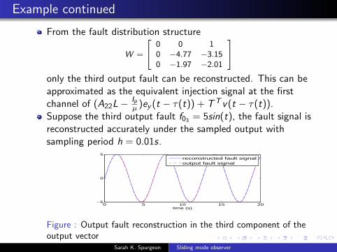
Example continued
From the fault distribution structure
W =
0 0 10 −4.77 −3.150 −1.97 −2.01
only the third output fault can be reconstructed. This can beapproximated as the equivalent injection signal at the firstchannel of (A22L− Ip
µ )ey (t − τ(t)) + TT v(t − τ(t)).Suppose the third output fault f03 = 5sin(t), the fault signal isreconstructed accurately under the sampled output withsampling period h = 0.01s.
0 5 10 15 20−5
0
5
time (s)
reconstructed fault signaloutput fault signal
Figure : Output fault reconstruction in the third component of theoutput vector
Sarah K. Spurgeon Sliding mode observer
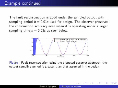
Example continued
The fault reconstruction is good under the sampled output withsampling period h = 0.01s used for design. The observer preservesthe construction accuracy even when it is operating under a largersampling time h = 0.03s as seen below.
0 5 10 15 20−2
−1
0
1
2
time (s)
reconstructed fault signalinput fault signal
Figure : Fault reconstruction using the proposed observer approach; theoutput sampling period is greater than that assumed in the design
Sarah K. Spurgeon Sliding mode observer
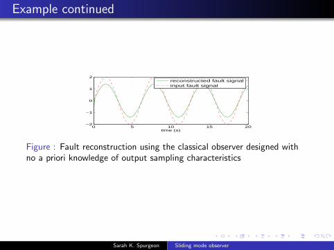
Example continued
0 5 10 15 20−2
−1
0
1
2
time (s)
reconstructed fault signalinput fault signal
Figure : Fault reconstruction using the classical observer designed withno a priori knowledge of output sampling characteristics
Sarah K. Spurgeon Sliding mode observer
Conclusions
The use of sliding mode observers in estimating faults andunknown parameters has been demonstrated.
A constructive fault reconstruction technique has beendemonstrated whereby the fault can be reconstructed reliablywhen the measured output is sampled.
Sarah K. Spurgeon Sliding mode observer

Sliding mode observers: higher order slidingmodes, complex systems and nonlinearity
Sarah K. Spurgeon
School of Engineering and Digital ArtsUniversity of Kent, UK
Spring School, Aussois, June 2015
Sarah K. Spurgeon Sliding mode observer

Sliding Mode Observers
Outline of Presentation
Sliding mode observer design for nonlinear systems - historicalperspective
Higher order sliding modes
Complex systems - decentralisation vs centralisation and theimpact on the observer design paradigm
Sarah K. Spurgeon Sliding mode observer
Sliding Mode Observers
Outline of Presentation
Sliding mode observer design for nonlinear systems - historicalperspective
Higher order sliding modes
Complex systems - decentralisation vs centralisation and theimpact on the observer design paradigm
Sarah K. Spurgeon Sliding mode observer

Sliding Mode Observers
Outline of Presentation
Sliding mode observer design for nonlinear systems - historicalperspective
Higher order sliding modes
Complex systems - decentralisation vs centralisation and theimpact on the observer design paradigm
Sarah K. Spurgeon Sliding mode observer

Sliding Mode Observers
Recap
We have developed constructive frameworks for observerdesign, particularly when systems can be approximated by alinear state-space model
We have yet to see translation of the core ideas into acomplex, system of system framework
We have not said anything about the implications of higherorder sliding modes on the observer paradigm
Sarah K. Spurgeon Sliding mode observer

Nonlinear sliding mode observers - historical perspective
Nonlinear system in companion form
x (n) = f (x , t) (1)
where f (x , t) is a nonlinear, uncertain function and x1 is themeasurement.
Slotine’s Observer
˙x1 = −α1e1 + x2 − k1sgn(e1) (2)˙x2 = −α2e1 + x3 − k2sgn(e1) (3)
.. .. .. (4)˙xn = −αne1 + f − knsgn(e1) (5)
αi chosen as for a Luenberger observer to ensure asymptoticerror decay when ki = 0
e1 = x1 − x1, f is an estimate of f (x , t)
Sarah K. Spurgeon Sliding mode observer

Slotine Nonlinear Observer
Error Dynamics
e1 = −α1e1 + e2 − k1sgn(e1) (6)
e2 = −α2e1 + e3 − k2sgn(e1) (7)
.. .. .. (8)
en = −αne1 + ∆f − knsgn(e1) (9)
∆f = f − f is assumed bounded and kn ≥| ∆f |
The sliding condition ddt (e1)2 < 0 is satisfied in the region
e2 ≤ k1 + α1e1 if e1 > 0
e2 ≥ −k1 + α1e1 if e1 < 0
Now revisit the error dynamics imposing the sliding condition.
Sarah K. Spurgeon Sliding mode observer
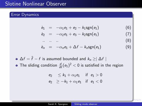
Slotine Nonlinear Observer
Error Dynamics
e1 = −α1e1 + e2 − k1sgn(e1) (6)
e2 = −α2e1 + e3 − k2sgn(e1) (7)
.. .. .. (8)
en = −αne1 + ∆f − knsgn(e1) (9)
∆f = f − f is assumed bounded and kn ≥| ∆f |The sliding condition d
dt (e1)2 < 0 is satisfied in the region
e2 ≤ k1 + α1e1 if e1 > 0
e2 ≥ −k1 + α1e1 if e1 < 0
Now revisit the error dynamics imposing the sliding condition.
Sarah K. Spurgeon Sliding mode observer
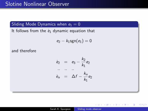
Slotine Nonlinear Observer
Sliding Mode Dynamics when e1 = 0
It follows from the e1 dynamic equation that
e2 − k1sgn(e1) = 0
and therefore
e2 = e3 −k2
k1e2
.. .. ..
en = ∆f − knk1
e2
What is the role of the observer gains?
Sarah K. Spurgeon Sliding mode observer

Slotine Nonlinear Observer
Sliding Mode Dynamics when e1 = 0
It follows from the e1 dynamic equation that
e2 − k1sgn(e1) = 0
and therefore
e2 = e3 −k2
k1e2
.. .. ..
en = ∆f − knk1
e2
What is the role of the observer gains?
Sarah K. Spurgeon Sliding mode observer
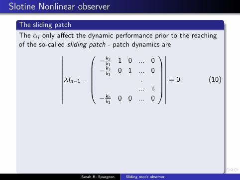
Slotine Nonlinear observer
The sliding patch
The αi only affect the dynamic performance prior to the reachingof the so-called sliding patch - patch dynamics are∣∣∣∣∣∣∣∣∣∣∣
λIn−1 −
−k2
k11 0 ... 0
−k3k1
0 1 ... 0
.... 1
−knk1
0 0 ... 0
∣∣∣∣∣∣∣∣∣∣∣= 0 (10)
Assuming kn is selected as a constant ratio with k1 and that thepoles defining the dynamics on the patch are critically damped i.e.are real and equal to some constant value γ, then∣∣∣e(i)
2
∣∣∣ ≤ (2γ)ik1 i = 0, ..., n − 2 (11)
from which the precision of the state estimates can be determined.
Sarah K. Spurgeon Sliding mode observer

Slotine Nonlinear observer
The sliding patch
The αi only affect the dynamic performance prior to the reachingof the so-called sliding patch - patch dynamics are∣∣∣∣∣∣∣∣∣∣∣
λIn−1 −
−k2
k11 0 ... 0
−k3k1
0 1 ... 0
.... 1
−knk1
0 0 ... 0
∣∣∣∣∣∣∣∣∣∣∣= 0 (10)
Assuming kn is selected as a constant ratio with k1 and that thepoles defining the dynamics on the patch are critically damped i.e.are real and equal to some constant value γ, then∣∣∣e(i)
2
∣∣∣ ≤ (2γ)ik1 i = 0, ..., n − 2 (11)
from which the precision of the state estimates can be determined.Sarah K. Spurgeon Sliding mode observer

Nonlinear observers- Further historical developments
Further Developments of Slotine
The effect of measurement noise on sliding mode observerswas formulated.
The system does not attain a sliding mode in the presence ofnoise, but remains within a region of the sliding patchdetermined by the bound on the noise.
Moreover, it was demonstrated that the average dynamics canbe modified by selection of the ki which in turn can tailor thecontribution of the noise to the state estimates.
Next steps
The equivalent injection design concept - Drakunov
Important as it is possible to develop an observer withoutusing input derivatives
Further developed by several authors
Sarah K. Spurgeon Sliding mode observer
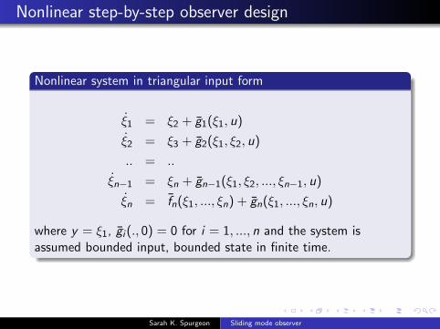
Nonlinear step-by-step observer design
Nonlinear system in triangular input form
ξ1 = ξ2 + g1(ξ1, u)
ξ2 = ξ3 + g2(ξ1, ξ2, u)
.. = ..
ξn−1 = ξn + gn−1(ξ1, ξ2, ..., ξn−1, u)
ξn = fn(ξ1, ..., ξn) + gn(ξ1, ..., ξn, u)
where y = ξ1, gi (., 0) = 0 for i = 1, ..., n and the system isassumed bounded input, bounded state in finite time.
Sarah K. Spurgeon Sliding mode observer
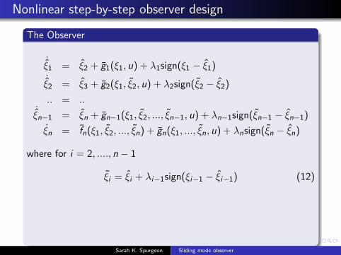
Nonlinear step-by-step observer design
The Observer
˙ξ1 = ξ2 + g1(ξ1, u) + λ1sign(ξ1 − ξ1)
˙ξ2 = ξ3 + g2(ξ1, ξ2, u) + λ2sign(ξ2 − ξ2)
.. = ..˙ξn−1 = ξn + gn−1(ξ1, ξ2, ..., ξn−1, u) + λn−1sign(ξn−1 − ξn−1)
ξn = fn(ξ1, ξ2, ..., ξn) + gn(ξ1, ..., ξn, u) + λnsign(ξn − ξn)
where for i = 2, ...., n − 1
ξi = ξi + λi−1sign(ξi−1 − ξi−1) (12)
Observation error information is not used before thecorresponding sliding manifold is reached
The manifolds are reached sequentially and ξi − ξi convergesto zero if the ξj − ξj with j < i have already converged to zero.
Sarah K. Spurgeon Sliding mode observer
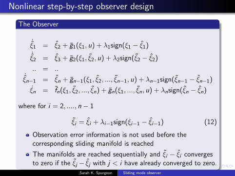
Nonlinear step-by-step observer design
The Observer
˙ξ1 = ξ2 + g1(ξ1, u) + λ1sign(ξ1 − ξ1)
˙ξ2 = ξ3 + g2(ξ1, ξ2, u) + λ2sign(ξ2 − ξ2)
.. = ..˙ξn−1 = ξn + gn−1(ξ1, ξ2, ..., ξn−1, u) + λn−1sign(ξn−1 − ξn−1)
ξn = fn(ξ1, ξ2, ..., ξn) + gn(ξ1, ..., ξn, u) + λnsign(ξn − ξn)
where for i = 2, ...., n − 1
ξi = ξi + λi−1sign(ξi−1 − ξi−1) (12)
Observation error information is not used before thecorresponding sliding manifold is reached
The manifolds are reached sequentially and ξi − ξi convergesto zero if the ξj − ξj with j < i have already converged to zero.
Sarah K. Spurgeon Sliding mode observer

Nonlinear step-by-step observer design
The error dynamics
e1 = e2 − λ1sign(ξ1 − ξ1)
e2 = e3 + g2(ξ1, ξ2, u)− g2(ξ1, ξ2, u)− λ2sign(ξ2 − ξ2)
.. = ..
en−1 = ξn − gn−1(ξ1, ξ2, ..., ξn−1, u)− λn−1sign(ξn−1 − ξn−1)
en = fn(ξ1, ..., ξn)− fn(ξ1, ξ2, ..., ξn) + gn(ξ1, ξ2, ..., ξn−1, u)−gn(ξ1, ..., ξn, u)− λnsign(ξn − ξn)
For sufficiently large λ1, a sliding mode is attained on e1 = 0 infinite time so that
e2 = λ1sign(ξ1 − ξ1)
which with (12) yields ξ2 = ξ2.
Sarah K. Spurgeon Sliding mode observer
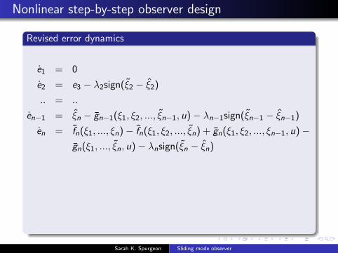
Nonlinear step-by-step observer design
Revised error dynamics
e1 = 0
e2 = e3 − λ2sign(ξ2 − ξ2)
.. = ..
en−1 = ξn − gn−1(ξ1, ξ2, ..., ξn−1, u)− λn−1sign(ξn−1 − ξn−1)
en = fn(ξ1, ..., ξn)− fn(ξ1, ξ2, ..., ξn) + gn(ξ1, ξ2, ..., ξn−1, u)−gn(ξ1, ..., ξn, u)− λnsign(ξn − ξn)
Proceeding as before it can be shown that for sufficiently large λ2,a sliding mode is then attained on e2 = 0 in finite time and itfollows that
e3 = λ2sign(ξ2 − ξ2)
which yields ξ3 = ξ3.
Sarah K. Spurgeon Sliding mode observer
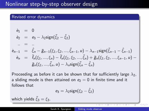
Nonlinear step-by-step observer design
Revised error dynamics
e1 = 0
e2 = e3 − λ2sign(ξ2 − ξ2)
.. = ..
en−1 = ξn − gn−1(ξ1, ξ2, ..., ξn−1, u)− λn−1sign(ξn−1 − ξn−1)
en = fn(ξ1, ..., ξn)− fn(ξ1, ξ2, ..., ξn) + gn(ξ1, ξ2, ..., ξn−1, u)−gn(ξ1, ..., ξn, u)− λnsign(ξn − ξn)
Proceeding as before it can be shown that for sufficiently large λ2,a sliding mode is then attained on e2 = 0 in finite time and itfollows that
e3 = λ2sign(ξ2 − ξ2)
which yields ξ3 = ξ3.
Sarah K. Spurgeon Sliding mode observer
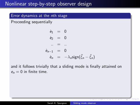
Nonlinear step-by-step observer design
Error dynamics at the nth stage
Proceeding sequentially
e1 = 0
e2 = 0
.. = ..
en−1 = 0
en = −λnsign(ξn − ξn)
and it follows trivially that a sliding mode is finally attained onen = 0 in finite time.
Many application specific studies of this step-by-step observerframework appear in the literature
The results were generalised to the MIMO case by Floquetand co-workers.
Sarah K. Spurgeon Sliding mode observer
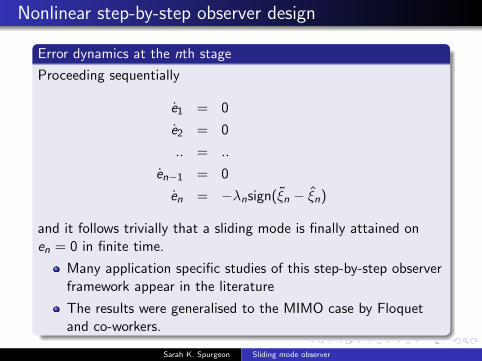
Nonlinear step-by-step observer design
Error dynamics at the nth stage
Proceeding sequentially
e1 = 0
e2 = 0
.. = ..
en−1 = 0
en = −λnsign(ξn − ξn)
and it follows trivially that a sliding mode is finally attained onen = 0 in finite time.
Many application specific studies of this step-by-step observerframework appear in the literature
The results were generalised to the MIMO case by Floquetand co-workers.
Sarah K. Spurgeon Sliding mode observer

Step-by step observer design and higher order slidingmodes
Step-by-step observer
The step-by-step procedure uses successive filtered values ofthe so-called equivalent output injections obtained fromrecursive first order sliding mode observers
The approximation of the equivalent injections by low passfilters at each step will typically introduce some delays thatlead to inaccurate estimates or to instability for high ordersystems
To overcome this problem, the discontinuous first order slidingmode output injection can be replaced by a continuous secondorder sliding mode injection
Sarah K. Spurgeon Sliding mode observer
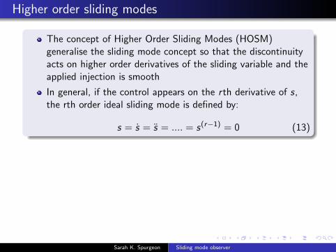
Higher order sliding modes
The concept of Higher Order Sliding Modes (HOSM)generalise the sliding mode concept so that the discontinuityacts on higher order derivatives of the sliding variable and theapplied injection is smooth
In general, if the control appears on the rth derivative of s,the rth order ideal sliding mode is defined by:
s = s = s = .... = s(r−1) = 0 (13)
A second order sliding mode injection - The super twistingalgorithm
ν(s) = φ(s) + λs |s|12 sign(s)
φ(s) = αssign(s)
λs , αs > 0
Sarah K. Spurgeon Sliding mode observer
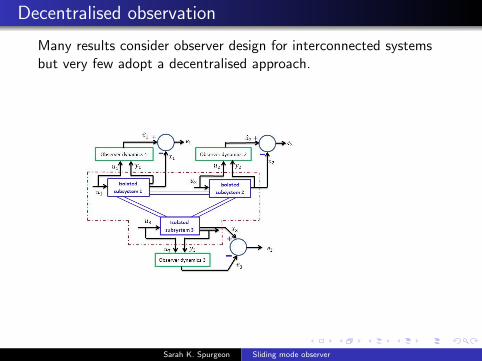
Decentralised observation
Many results consider observer design for interconnected systemsbut very few adopt a decentralised approach.
Sarah K. Spurgeon Sliding mode observer
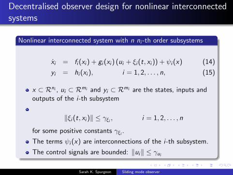
Decentralised observer design for nonlinear interconnectedsystems
Nonlinear interconnected system with n ni -th order subsystems
xi = fi (xi ) + gi (xi ) (ui + ξi (t, xi )) + ψi (x) (14)
yi = hi (xi ), i = 1, 2, . . . , n, (15)
x ⊂ Rni , ui ⊂ Rmi and yi ⊂ Rmi are the states, inputs andoutputs of the i-th subsystem
‖ξi (t, xi )‖ ≤ γξi , i = 1, 2, . . . , n
for some positive constants γξi .
The terms ψi (x) are interconnections of the i-th subsystem.
The control signals are bounded: ‖ui‖ ≤ γui
Sarah K. Spurgeon Sliding mode observer

Decentralised observer design for nonlinear interconnectedsystems
Design Objective
To design n ni -th order dynamical systems
˙xi = Φi (t, xi , yi , ui ), i = 1, 2, . . . , n (16)
where xi ∈ Rni , such that the solutions xi (t) of system (16) areconvergent to xi (t) exponentially for i = 1, 2, . . . , n, that is, thereexist constants αi > 0 and βi > 0 such that
‖xi (t)− xi (t)‖ ≤ αi exp−βi t, i = 1, 2, . . . , n
where xi (t) are the solutions of the interconnected systems(14)–(15).
The systems in (16) comprise an exponential observer for theinterconnected system (14)–(15).
Sarah K. Spurgeon Sliding mode observer
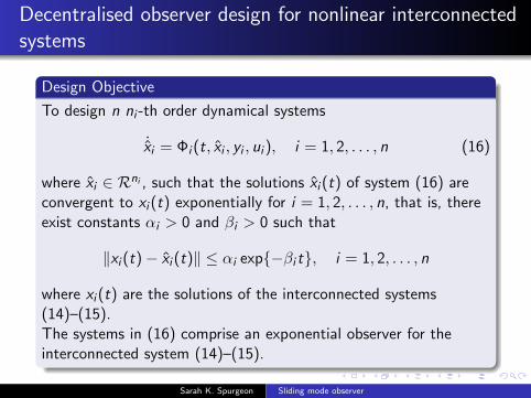
Decentralised observer design for nonlinear interconnectedsystems
Design Objective
To design n ni -th order dynamical systems
˙xi = Φi (t, xi , yi , ui ), i = 1, 2, . . . , n (16)
where xi ∈ Rni , such that the solutions xi (t) of system (16) areconvergent to xi (t) exponentially for i = 1, 2, . . . , n, that is, thereexist constants αi > 0 and βi > 0 such that
‖xi (t)− xi (t)‖ ≤ αi exp−βi t, i = 1, 2, . . . , n
where xi (t) are the solutions of the interconnected systems(14)–(15).The systems in (16) comprise an exponential observer for theinterconnected system (14)–(15).
Sarah K. Spurgeon Sliding mode observer
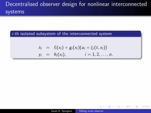
Decentralised observer design for nonlinear interconnectedsystems
i-th isolated subsystem of the interconnected system
xi = fi (xi ) + gi (xi )(ui + ξi (t, xi ))
yi = hi (xi ), i = 1, 2, . . . , n,
i-th nominal isolated subsystem of the interconnected system
xi = fi (xi ) + gi (xi )ui (17)
yi = hi (xi ), i = 1, 2, . . . , n, (18)
Sarah K. Spurgeon Sliding mode observer
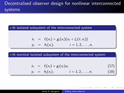
Decentralised observer design for nonlinear interconnectedsystems
i-th isolated subsystem of the interconnected system
xi = fi (xi ) + gi (xi )(ui + ξi (t, xi ))
yi = hi (xi ), i = 1, 2, . . . , n,
i-th nominal isolated subsystem of the interconnected system
xi = fi (xi ) + gi (xi )ui (17)
yi = hi (xi ), i = 1, 2, . . . , n, (18)
Sarah K. Spurgeon Sliding mode observer
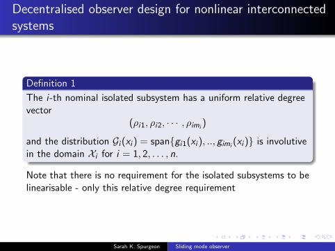
Decentralised observer design for nonlinear interconnectedsystems
Definition 1
The i-th nominal isolated subsystem has a uniform relative degreevector
(ρi1, ρi2, · · · , ρimi)
and the distribution Gi (xi ) = spangi1(xi ), .., gimi(xi ) is involutive
in the domain Xi for i = 1, 2, . . . , n.
Note that there is no requirement for the isolated subsystems to belinearisable - only this relative degree requirement
Sarah K. Spurgeon Sliding mode observer

Decentralised observer design for nonlinear interconnectedsystems
Exploiting structure - Canonical Form for Design 1
Let ρi :=∑mi
j=1 ρij for i = 1, 2, . . . n. From Assumption 1, the
differentials dhij(xi ), dLfihij(xi ), · · · , dLρij−1fi
hij(xi ) are linearlyindependent for j = 1, . . . ,mi and i = 1, . . . , n. Let
zij =
hij(xi )
Lfihij(xi )...
Lρij−1fi
hij(xi )
:= zij(xi ), j = 1, 2, . . . ρi (19)
for i = 1, . . . , n. Since the Gi (xi ) are involutive, there exist ni − ρifunctions wi1, · · · , wi(ni−ρi ) such that the Jacobian matrix of thefollowing mapping is nonsingular:
Ti : xi 7→ col(zi1, · · · , ziρi ,wi1, · · · ,wi(ni−ρi )) (20)Sarah K. Spurgeon Sliding mode observer

Decentralised observer design for nonlinear interconnectedsystems
Exploiting structure - Canonical Form for Design 2
The transformations col(zi ,wi ) = Ti (xi ) are diffeomorphisms. Let
T (x) :=
T1(x1)T2(x2)
...Tn(xn)
(21)
It is clear that T (x) defines a new coordinate system col(z1, w1,z2,w2, · · · , zn,wn).
Sarah K. Spurgeon Sliding mode observer
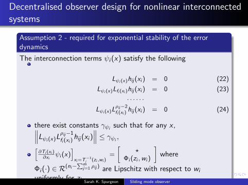
Decentralised observer design for nonlinear interconnectedsystems
Assumption 2 - required for exponential stability of the errordynamics
The interconnection terms ψi (x) satisfy the following
Lψi (x)hij(xi ) = 0 (22)
Lψi (x)Lfi (xi )hij(xi ) = 0 (23)
· · · · · ·Lψi (x)L
ρij−2fi (xi )
hij(xi ) = 0 (24)
there exist constants γψisuch that for any x ,∥∥∥Lψi (x)L
ρij−1
fi (xi )hij(xi )
∥∥∥ ≤ γψi,[
∂Ti (xi )∂xi
ψi (x)]xi=T−1
i (zi ,wi )=
[?
Φi (zi ,wi )
]where
Φi (·) ∈ R(ni−∑m
j=1 ρij ) are Lipschitz with respect to wi
uniformly for zi Sarah K. Spurgeon Sliding mode observer
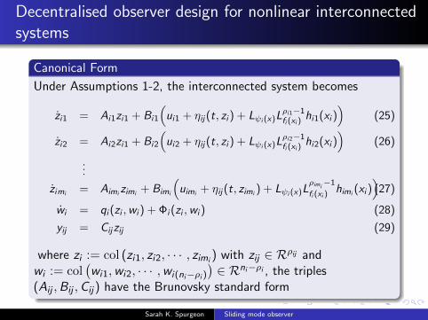
Decentralised observer design for nonlinear interconnectedsystems
Canonical Form
Under Assumptions 1-2, the interconnected system becomes
zi1 = Ai1zi1 + Bi1
(ui1 + ηij(t, zi ) + Lψi (x)L
ρi1−1fi (xi )
hi1(xi ))
(25)
zi2 = Ai2zi1 + Bi2
(ui2 + ηij(t, zi ) + Lψi (x)L
ρi2−1fi (xi )
hi2(xi ))
(26)
...
zimi = Aimi zimi + Bimi
(uimi + ηij(t, zimi ) + Lψi (x)L
ρimi−1
fi (xi )himi (xi )
)(27)
wi = qi (zi ,wi ) + Φi (zi ,wi ) (28)
yij = Cijzij (29)
where zi := col (zi1, zi2, · · · , zimi) with zij ∈ Rρij and
wi := col(wi1,wi2, · · · ,wi(ni−ρi )
)∈ Rni−ρi , the triples
(Aij ,Bij ,Cij) have the Brunovsky standard form
Sarah K. Spurgeon Sliding mode observer

Decentralised observer design for nonlinear interconnectedsystems
HOSM-based decentralised observer design
The i-th subsystem of (25)-(27) can be written as
zij = Aijzi + Bij
(uij + ηij(t, zi ) + Lψi (x)L
ρij−1fi (xi )
hij(xi )), (30)
yij(t) = zij1(t) := hij(xi (t)) (31)
Consider the higher order sliding surfaces defined by
sij = Lgi sij = L2gisij = · · · = L
ρijgi sij = 0
where sij(t) := zij1(t)− yij(t) and zij1 is determined by a HOSMdifferentiator scheme
Sarah K. Spurgeon Sliding mode observer

Decentralised observer design for nonlinear interconnectedsystems
HOSM Differentiator
˙zij1 = νij1 (32)
νij1 = −λij1 |sij |ρij−1
ρij sign(sij) + zij1 (33)
...˙zij(ρij−1) = νij(ρij−1) (34)
νij(ρij−1) = −λij(ρij−1) |zij(ρij−1) − νij(ρij−2)|12
sign(zij(ρij−1) − νij(ρij−2)) + zijρij (35)
˙zijρij = −λijρij sign(zijρij − νij(ρij−1)) (36)
where λijk are positive parameters for i = 1, 2, . . . , n,j = 1, 2, . . . ,mi and k = 1, 2, . . . , ρij .
Sarah K. Spurgeon Sliding mode observer
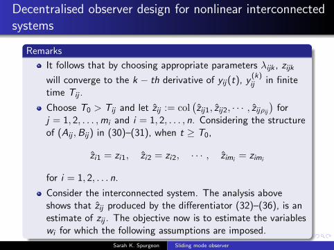
Decentralised observer design for nonlinear interconnectedsystems
Remarks
It follows that by choosing appropriate parameters λijk , zijk
will converge to the k − th derivative of yij(t), y(k)ij in finite
time Tij .
Choose T0 > Tij and let zij := col(zij1, zij2, · · · , zijρij
)for
j = 1, 2, . . . ,mi and i = 1, 2, . . . , n. Considering the structureof (Aij ,Bij) in (30)–(31), when t ≥ T0,
zi1 = zi1, zi2 = zi2, · · · , zimi= zimi
for i = 1, 2, . . . n.
Consider the interconnected system. The analysis aboveshows that zij produced by the differentiator (32)–(36), is anestimate of zij . The objective now is to estimate the variableswi for which the following assumptions are imposed.
Sarah K. Spurgeon Sliding mode observer
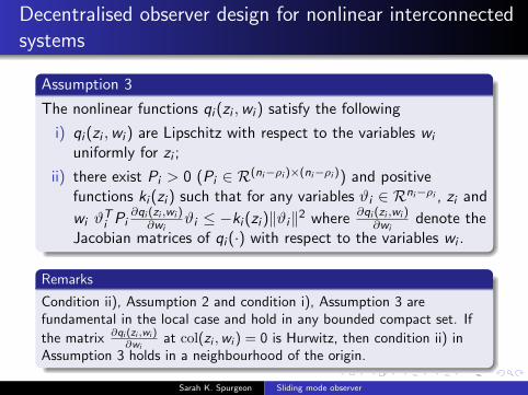
Decentralised observer design for nonlinear interconnectedsystems
Assumption 3
The nonlinear functions qi (zi ,wi ) satisfy the following
i) qi (zi ,wi ) are Lipschitz with respect to the variables wi
uniformly for zi ;
ii) there exist Pi > 0 (Pi ∈ R(ni−ρi )×(ni−ρi )) and positivefunctions ki (zi ) such that for any variables ϑi ∈ Rni−ρi , zi and
wi ϑTi Pi
∂qi (zi ,wi )∂wi
ϑi ≤ −ki (zi )‖ϑi‖2 where ∂qi (zi ,wi )∂wi
denote theJacobian matrices of qi (·) with respect to the variables wi .
Remarks
Condition ii), Assumption 2 and condition i), Assumption 3 arefundamental in the local case and hold in any bounded compact set. If
the matrix ∂qi (zi ,wi )∂wi
at col(zi ,wi ) = 0 is Hurwitz, then condition ii) inAssumption 3 holds in a neighbourhood of the origin.
Sarah K. Spurgeon Sliding mode observer
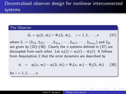
Decentralised observer design for nonlinear interconnectedsystems
The Observer
˙wi = qi (zi , wi ) + Φi (zi , wi ), i = 1, 2, · · · , n (37)
where zi := (zi11, zi12, · · · , zi1ρi1 , · · · , zimi1, · · · , zimiρi1) and zijkare given by (32)–(36). Clearly the n systems defined in (37) aredecoupled from each other. Let ei (t) = wi (t)− wi (t). It followsfrom Assumption 2 that the error dynamics are described by
ei = qi (zi ,wi )− qi (zi , wi ) + Φi (zi ,wi )− Φj(zi , wi ) (38)
for i = 1, 2, . . . , n.
Sarah K. Spurgeon Sliding mode observer

Decentralised observer design for nonlinear interconnectedsystems
Theorem
Under Assumptions 1–3, the error dynamical system (38) isexponentially stable if for i = 1, 2, . . . , n
infzi
ki (zi )− ‖Pi‖LΦi
(zi )
:= βi > 0 (39)
where Pi and ki (zi ) satisfy Assumption 3 and Φi (zi ) are given inAssumption 2.
Sarah K. Spurgeon Sliding mode observer
Decentralised observer design for nonlinear interconnectedsystems
Remarks
From Levant HOSM algorithm, the variables zi converge to ziin finite time. Theorem 1 shows that the variables wi
converges to w exponentially. The HOSM differentiator andthe designed dynamics together form the exponential observer.
From the structure of the designed dynamical system and thestructure of Levant differentiator, it is straightforward to seethat the designed dynamics are decoupled and thus thedesigned observers are decentralised.
Sarah K. Spurgeon Sliding mode observer

Sliding Mode Observers
Concluding Remarks
We have developed an exponential observer which exploitsstructure in the design including mismatched uncertainty
HOSM and sliding mode differentiators have been introduced
Demonstrated that the sliding mode observer paradigmtranslates to nonlinear and complex system scenarios
Sarah K. Spurgeon Sliding mode observer