reduced order observers
TRANSCRIPT
Reduced Order Observers for Linear Systems
SOLO HERMELIN
Updated: 08.12.08
Table of Content
SOLO Reduced Order Observers for Linear Systems
SOLO Reduced Order Observers for Linear Systems
∈∈∈+=∈∈∈∈+=
pxmpxnpx
nxmnxnmxnx
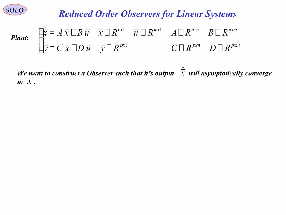
RDRCRyuDxCy
RBRARuRxuBxAx1
11Plant:
We want to construct a Observer such that it’s output will asymptotically convergeto .x
x̂
SOLO Reduced Order Observers for Linear Systems
∈∈∈+=∈∈∈∈+=
pxmpxnpx
nxmnxnmxnx
RDRCRyuDxCy
RBRARuRxuBxAx1
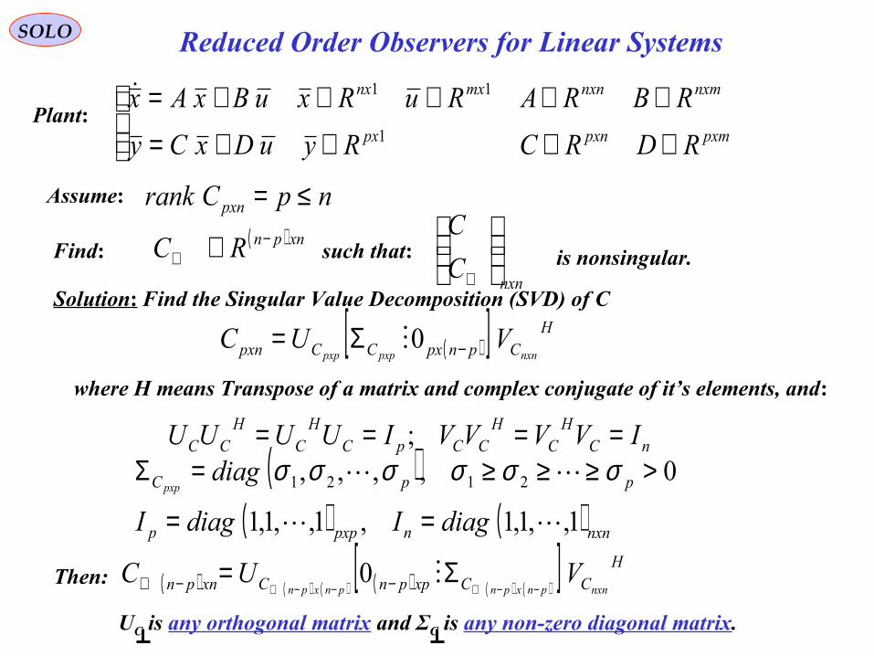
11Plant:
Assume: npCrank pxn ≤=
Find:( ) xnpnRC −
⊥ ∈ such that:
nxnC
C
⊥is nonsingular.
Solution: Find the Singular Value Decomposition (SVD) of C
( )[ ] HCpnpxCCpxn nxnpxppxpVUC −Σ= 0
where H means Transpose of a matrix and complex conjugate of it’s elements, and:
nCH
CH
CCpCH
CH
CC IVVVVIUUUU ==== ;( )
( ) ( ) nxnnpxpp
ppC
diagIdiagI
diagpxp
1,,1,1,1,,1,1
0,,,, 2121
==
>≥≥≥=Σ σσσσσσ
( ) ( ) ( ) ( ) ( ) ( )[ ] H
CCxppnCxnpn nxnpnxpnpnxpnVUC
−−⊥−−⊥Σ= −−⊥ 0Then:
UC is any orthogonal matrix and ΣC is any non-zero diagonal matrix.
SOLO Reduced Order Observers for Linear Systems
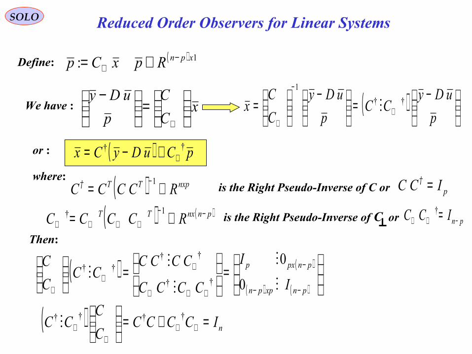
Define:
We have : xC
C
p
uDy
=
−
⊥
( ) 1: xpnRpxCp −⊥ ∈=
( )
−=
−
= ⊥
−
⊥ p
uDyCC
p
uDy
C
Cx ††
1
or : ( ) pCuDyCx ††⊥+−=
where: ( ) nxpTT RCCCC ∈= −1† is the Right Pseudo-Inverse of C or pICC =†
( ) ( )pnnxTT RCCCC −−⊥⊥⊥⊥ ∈= 1† is the Right Pseudo-Inverse of C or pnICC −⊥⊥ =†
Then:
( ) ( )
( ) ( )
=
=
−−
−
⊥⊥⊥
⊥⊥
⊥ pnxppn
pnpxp
I
I
CCCC
CCCCCC
C
C
0
0††
††††
( ) nICCCCC
CCC =+=
⊥⊥
⊥⊥
††††
SOLO Reduced Order Observers for Linear Systems
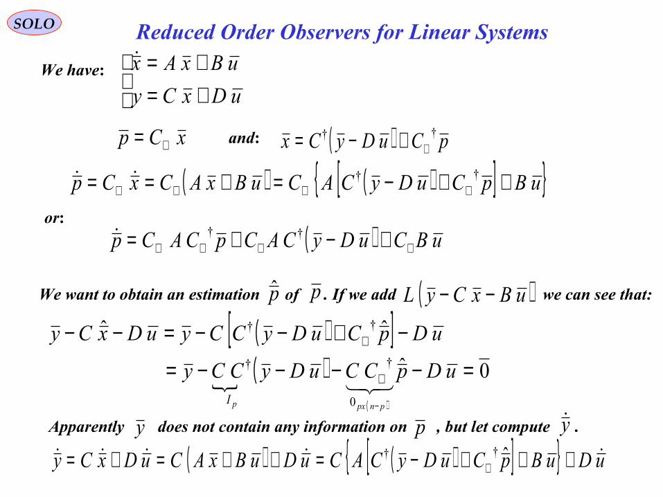
We have:
+=+=
uDxCy
uBxAx
( ) pCuDyCx ††⊥+−=and:xCp ⊥=
( ) ( )[ ]{ }uBpCuDyCACuBxACxCp ++−=+== ⊥⊥⊥⊥††
or:
( ) uBCuDyCACpCACp ⊥⊥⊥⊥ +−+= ††
We want to obtain an estimation of . If we add we can see that:pp̂ ( )uBxCyL −−
( )[ ] ( )
( )
0ˆ
ˆˆ
0
††
††
=−−−−=
−+−−=−−
−
⊥
⊥
uDpCCuDyCCy
uDpCuDyCCyuDxCy
pnpxpI
Apparently does not contain any information on , but let compute .py y
( ) ( )[ ]{ } uDuBpCuDyCACuDuBxACuDxCy +++−=++=+= ⊥ˆ††
SOLO Reduced Order Observers for Linear Systems
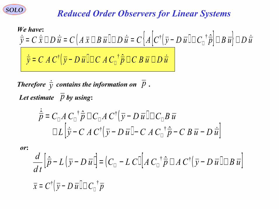
We have:
Therefore contains the information on .py
( ) ( )[ ]{ } uDuBpCuDyCACuDuBxACuDxCy +++−=++=+= ⊥ˆ††
( ) uDuBCpCACuDyCACy +++−= ⊥ˆ††
Let estimate by using:p
( )( )[ ]uDuBCpCACuDyCACyL
uBCuDyCACpCACp
−−−−−+
+−+=
⊥
⊥⊥⊥⊥
ˆ
ˆˆ
††
††
or:
( )[ ] ( ) ( )[ ]uBuDyCApCACLCuDyLptd
d +−+−=−− ⊥⊥†† ˆˆ
( ) pCuDyCx ††⊥+−=

SOLO Reduced Order Observers for Linear Systems
We have:
( )[ ] ( ) ( )[ ]uBuDyCApCACLCuDyLptd
d +−+−=−− ⊥⊥†† ˆˆ
( ) pCuDyCx ˆˆ ††⊥+−=
SOLO Reduced Order Observers for Linear Systems
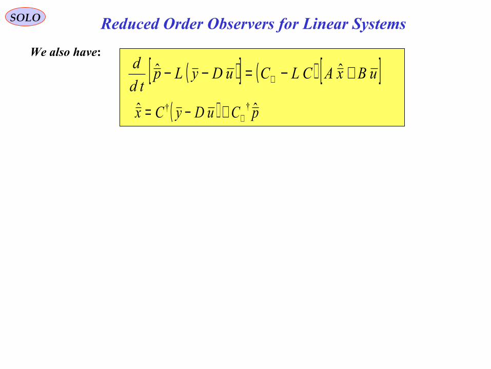
We also have:
( )[ ] ( ) [ ]uBxACLCuDyLptd
d +−=−− ⊥ˆˆ
( ) pCuDyCx ˆˆ ††⊥+−=
SOLO Reduced Order Observers for Linear Systems
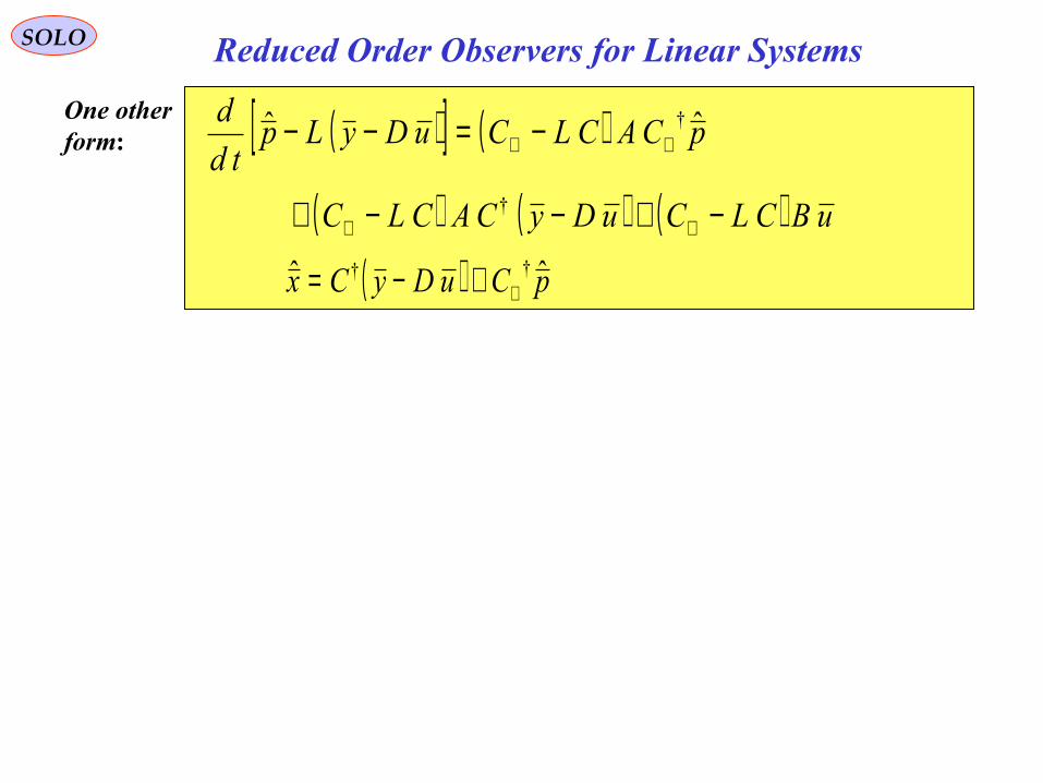
One otherform: ( )[ ] ( )
( ) ( ) ( ) uBCLCuDyCACLC
pCACLCuDyLptd
d
−+−−+
−=−−
⊥⊥
⊥⊥
†
† ˆˆ
( ) pCuDyCx ˆˆ ††⊥+−=
SOLO Reduced Order Observers for Linear Systems
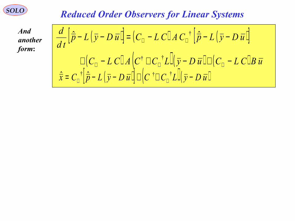
Andanotherform:
( )[ ] ( ) ( )[ ]( ) ( ) ( ) ( ) uBCLCuDyLCCACLC
uDyLpCACLCuDyLptd
d
−+−+−+
−−−=−−
⊥⊥⊥
⊥⊥
††
† ˆˆ
( )[ ] ( ) ( )uDyLCCuDyLpCx −++−−= ⊥⊥††† ˆˆ
SOLO Reduced Order Observers for Linear Systems
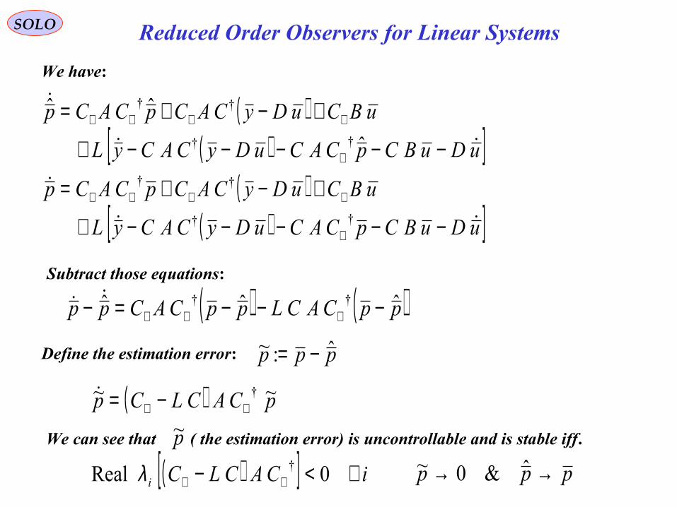
We have:
( )( )[ ]uDuBCpCACuDyCACyL
uBCuDyCACpCACp
−−−−−+
+−+=
⊥
⊥⊥⊥⊥
ˆ
ˆˆ
††
††
Subtract those equations:
Define the estimation error:
( )( )[ ]uDuBCpCACuDyCACyL
uBCuDyCACpCACp
−−−−−+
+−+=
⊥
⊥⊥⊥⊥††
††
( ) ( )ppCACLppCACpp ˆˆˆ †† −−−=− ⊥⊥⊥
ppp ˆ:~ −=
( ) pCACLCp ~~ †⊥⊥ −=
p~We can see that ( the estimation error) is uncontrollable and is stable iff.
( )[ ] iCACLCi ∀<− ⊥⊥ 0Real †λ ppp →→ ˆ&0~
SOLO Reduced Order Observers for Linear Systems
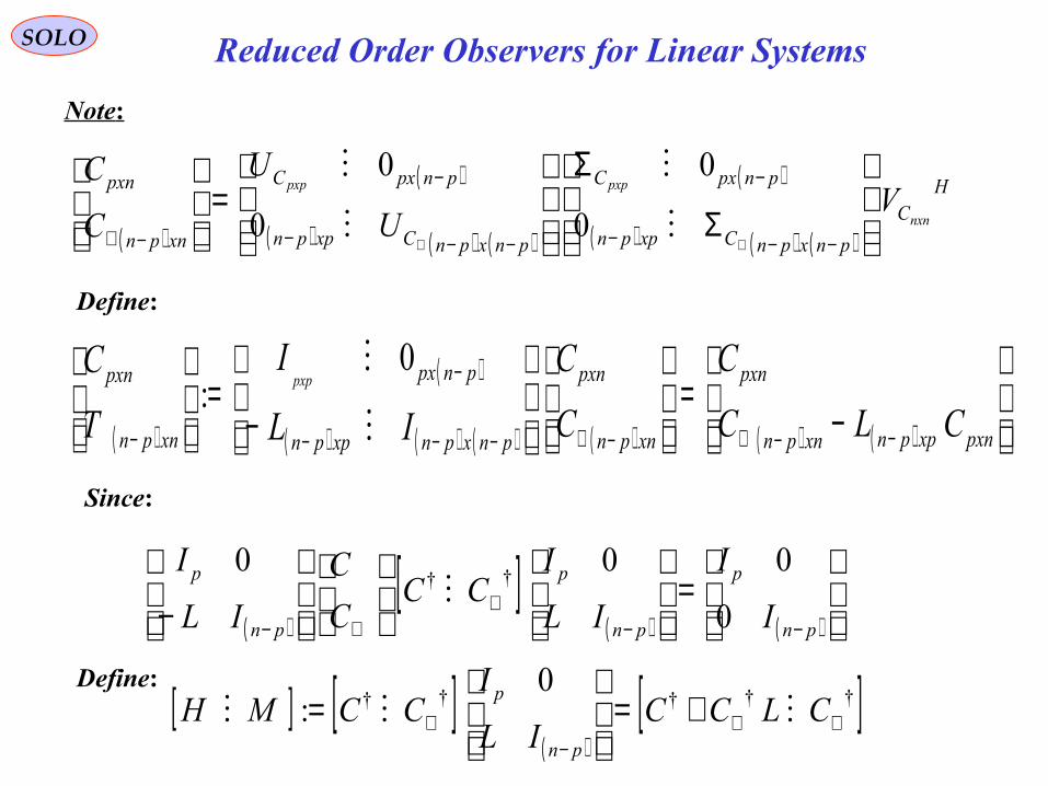
Note:
Define:
( )
( )
( ) ( ) ( )
( )
( ) ( ) ( )
HC
pnxpnCxppn
pnpxC
pnxpnCxppn
pnpxC
xnpn
pxn
nxn
pxppxp
VU
U
C
C
Σ
Σ
=
−−−
−
−−−
−
−⊥ ⊥⊥
0
0
0
0
( )
( )
( ) ( ) ( ) ( ) ( ) ( )
−
=
−=
−−⊥−⊥−−−
−
− pxnxppnxnpn
pxn
xnpn
pxn
pnxpnxppn
pnpx
xnpn
pxn
CLC
C
C
C
IL
I
T
Cpxp
0:
Since:
( )[ ]
( ) ( )
=
− −−
⊥⊥− pn
p
pn
p
pn
p
I
I
IL
ICC
C
C
IL
I
0
000††
Define:[ ] [ ]
( )[ ]†††††
0: ⊥⊥
−⊥ +=
= CLCC
IL
ICCMH
pn
p
SOLO Reduced Order Observers for Linear Systems
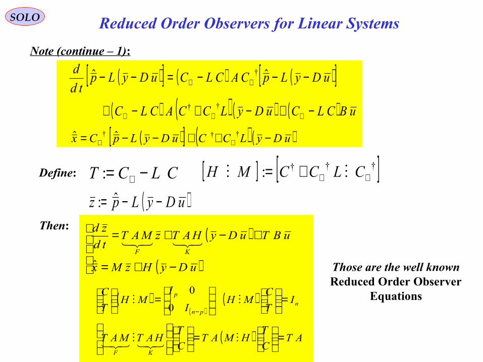
Note (continue – 1):
Define: CLCT −= ⊥:
Then:
( )[ ] ( ) ( )[ ]( ) ( ) ( ) ( ) uBCLCuDyLCCACLC
uDyLpCACLCuDyLptd
d
−+−+−+
−−−=−−
⊥⊥⊥
⊥⊥
††
† ˆˆ
( )[ ] ( ) ( )uDyLCCuDyLpCx −++−−= ⊥⊥††† ˆˆ
[ ] [ ]†††: ⊥⊥+= CLCCMH
( )uDyLpz −−= ˆ:
( )
( )
−+=
+−+=
uDyHzMx
uBTuDyHATzMATtd
zd
KF
ˆ
( )( )
( )
( ) ATC
THMAT
C
THATMAT
IT
CMH
I
IMH
T
C
KF
npn
p
=
=
=
=
−
0
0
Those are the well knownReduced Order Observer
Equations
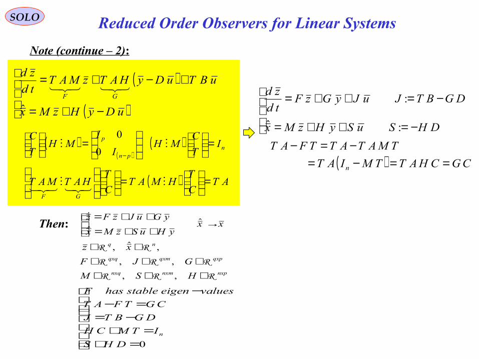
SOLO Reduced Order Observers for Linear Systems
Note (continue – 2):
Then:
( )
( )
−+=
+−+=
uDyHzMx
uBTuDyHATzMATtd
zd
GF
ˆ
( )( )
( )
( ) ATC
THMAT
C
THATMAT
IT
CMH
I
IMH
T
C
GF
npn
p
=
=
=
=
−
0
0
( ) CGCHATTMIAT
TMATATTFAT
DHSuSyHzMx
DGBTJuJyGzFtd
zd
n ==−=−=−
−=++=
−=++=
:ˆ
:
=+=+
−==−
−
0DHS
ITMCH
DGBTJ
CGTFAT
valueseigenstablehasF
n
nxpnxmnxq
qxpqxmqxq
nq
HSM
GJF
xz
xxyHuSzMx
yGuJzFz
RRR
RRR
RR
∈∈∈∈∈∈
∈∈
→
++=
++=
,,
,,
,ˆ,
ˆˆ
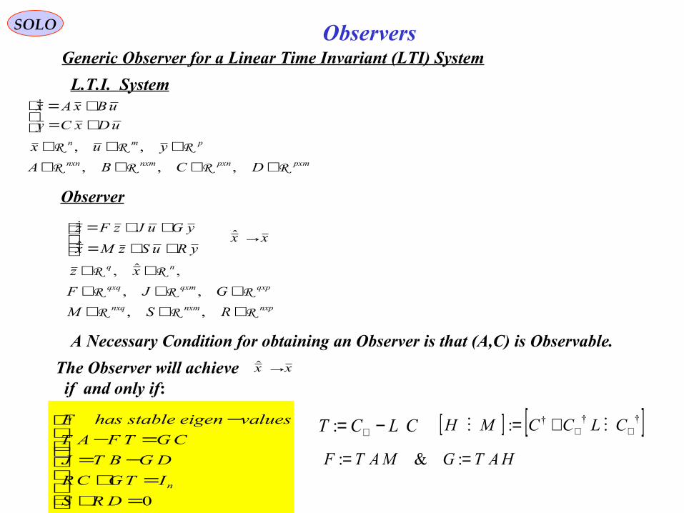
SOLO ObserversGeneric Observer for a Linear Time Invariant (LTI) System
pxmpxnnxmnxn
pmn
DCBA
yux
uDxCy
uBxAx
RRRR
RRR
∈∈∈∈∈∈∈
+=+=
,,,
,,
Observer
nxpnxmnxq
qxpqxmqxq
nq
RSM
GJF
xz
xxyRuSzMx
yGuJzFz
RRR
RRR
RR
∈∈∈∈∈∈
∈∈
→
++=
++=
,,
,,
,ˆ,
ˆˆ
A Necessary Condition for obtaining an Observer is that (A,C) is Observable.
The Observer will achieve if and only if:
xx →ˆ
=+=+
−==−
−
0DRS
ITGCR
DGBTJ
CGTFAT
valueseigenstablehasF
n
L.T.I. System
[ ] [ ]†††: ⊥⊥+= CLCCMH CLCT −= ⊥:
HATGMATF == :&:
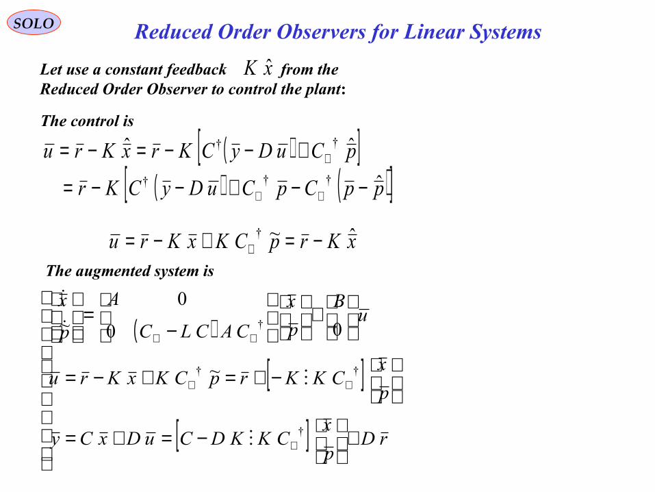
SOLO Reduced Order Observers for Linear Systems
Let use a constant feedback from theReduced Order Observer to control the plant:
xK ˆ
The control is
xKrpCKxKru ˆ~† −=+−= ⊥
( )[ ]( ) ( )[ ]ppCpCuDyCKr
pCuDyCKrxKru
ˆ
ˆˆ
†††
††
−−+−−=
+−−=−=
⊥⊥
⊥
The augmented system is
( )
[ ]
[ ]
+
−=+=
−+=+−=
+
−
=
⊥
⊥⊥
⊥⊥
rDp
xCKKDCuDxCy
p
xCKKrpCKxKru
uB
p
x
CACLC
A
p
x
†
††
†
~
00
0~
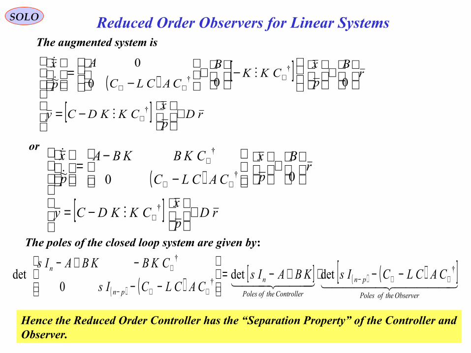
SOLO Reduced Order Observers for Linear SystemsThe augmented system is
( )[ ]
[ ]
+
−=
+
−
+
−=
⊥
⊥⊥⊥
rDp
xCKKDCy
rB
p
xCKK
B
CACLC
A
p
x
†
†
† 000
0~
or
The poles of the closed loop system are given by:
( )
[ ]
+
−=
+
−
−=
⊥
⊥⊥
⊥
rDp
xCKKDCy
rB
p
x
CACLC
CKBKBA
p
x
†
†
†
00~
( ) ( )[ ] ( ) ( )[ ]
ObservertheofPoles
pn
ControllertheofPoles
n
pn
nCACLCIsKBAIs
CACLCIs
CKBKBAIs †
†
†
detdet0
det ⊥⊥−⊥⊥−
⊥ −−⋅+−=
−−
−+−
Hence the Reduced Order Controller has the “Separation Property” of the Controller andObserver.
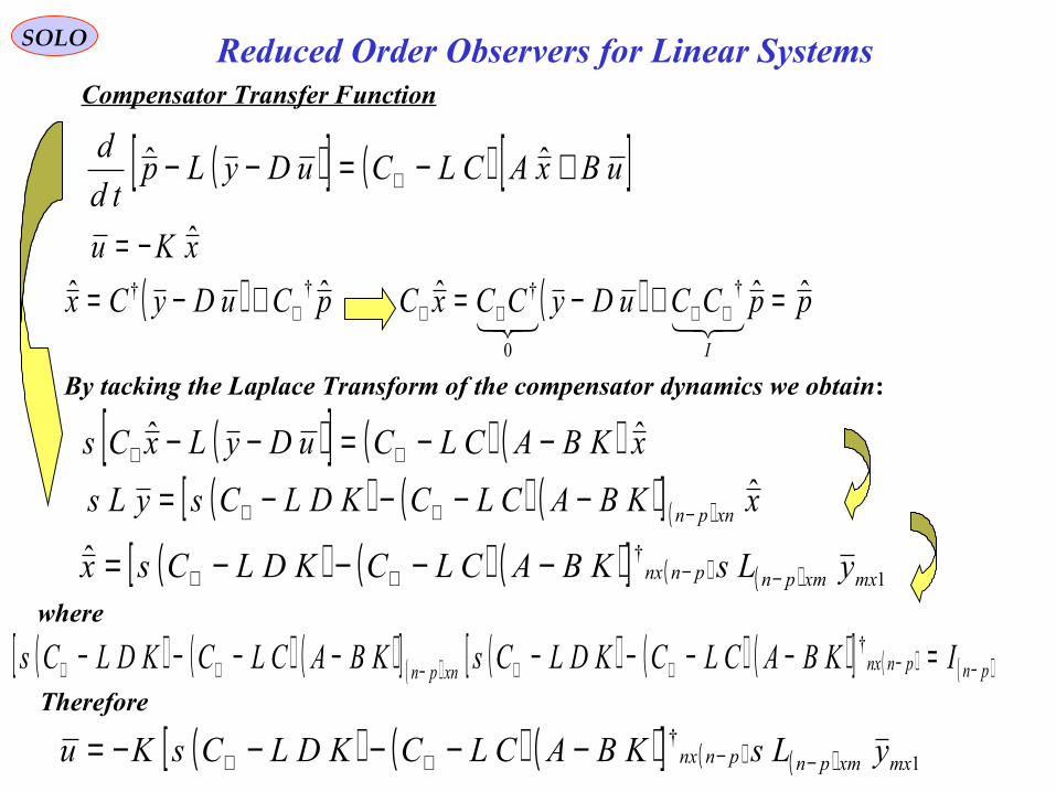
SOLO Reduced Order Observers for Linear SystemsCompensator Transfer Function
By tacking the Laplace Transform of the compensator dynamics we obtain:
( )[ ] ( ) [ ]uBxACLCuDyLptd
d +−=−− ⊥ˆˆ
( ) pCuDyCx ˆˆ ††⊥+−=
xKu ˆ−=( ) ppCCuDyCCxC
I
ˆˆˆ †
0
† =+−= ⊥⊥⊥⊥
( )[ ] ( ) ( ) xKBACLCuDyLxCs ˆˆ −−=−− ⊥⊥
( ) ( ) ( )[ ] ( ) xKBACLCKDLCsyLs xnpnˆ
−⊥⊥ −−−−=
( ) ( ) ( )[ ] ( ) ( ) 1†ˆ
mxxmpnpnnx yLsKBACLCKDLCsx −−⊥⊥ −−−−=where
Therefore
( ) ( ) ( )[ ] ( ) ( ) ( ) ( )[ ] ( ) ( )pnpnnxxnpn IKBACLCKDLCsKBACLCKDLCs −−⊥⊥−⊥⊥ =−−−−−−−− †
( ) ( ) ( )[ ] ( ) ( ) 1†
mxxmpnpnnx yLsKBACLCKDLCsKu −−⊥⊥ −−−−−=
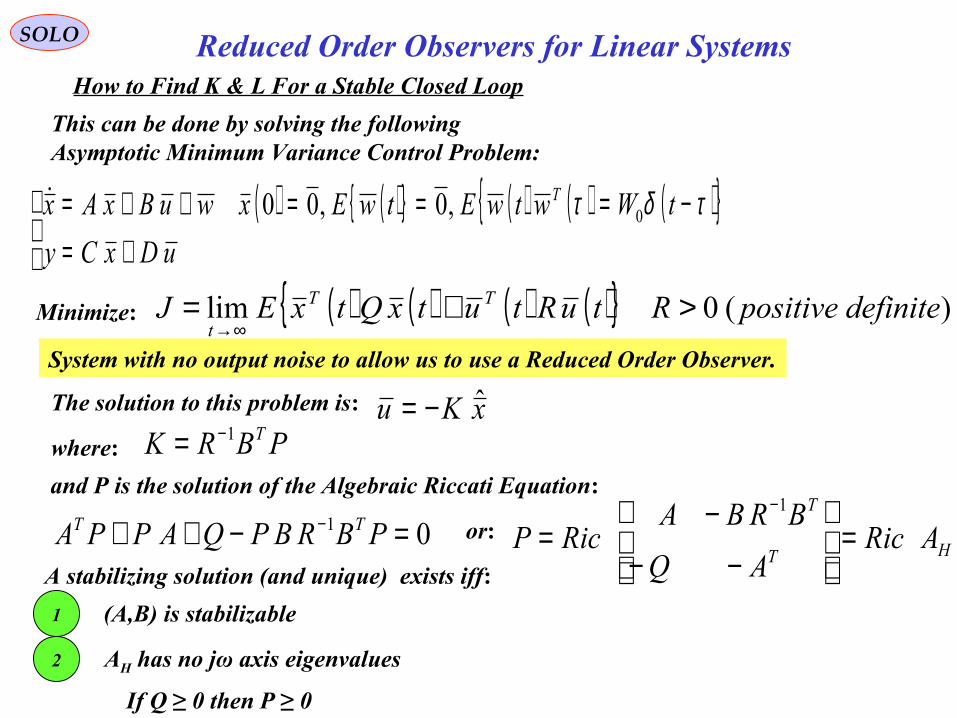
SOLO Reduced Order Observers for Linear SystemsHow to Find K & L For a Stable Closed Loop
This can be done by solving the followingAsymptotic Minimum Variance Control Problem:
xKu ˆ−=
( ) ( ){ } ( ) ( ) ( ){ }
+=−===++=
uDxCy
tWwtwEtwExwuBxAx T τδτ 0,0,00
( ) ( ) ( ) ( ){ } )(0lim definitepositiveRtuRtutxQtxEJ TT
t>+=
∞→
System with no output noise to allow us to use a Reduced Order Observer.
The solution to this problem is:
where: PBRK T1−=and P is the solution of the Algebraic Riccati Equation:
01 =−++ − PBRBPQAPPA TT or:HT
T
ARicAQ
BRBARicP =
−−−
=−1
Minimize:
A stabilizing solution (and unique) exists iff:
1 (A,B) is stabilizable
2 AH has no jω axis eigenvalues
If Q ≥ 0 then P ≥ 0
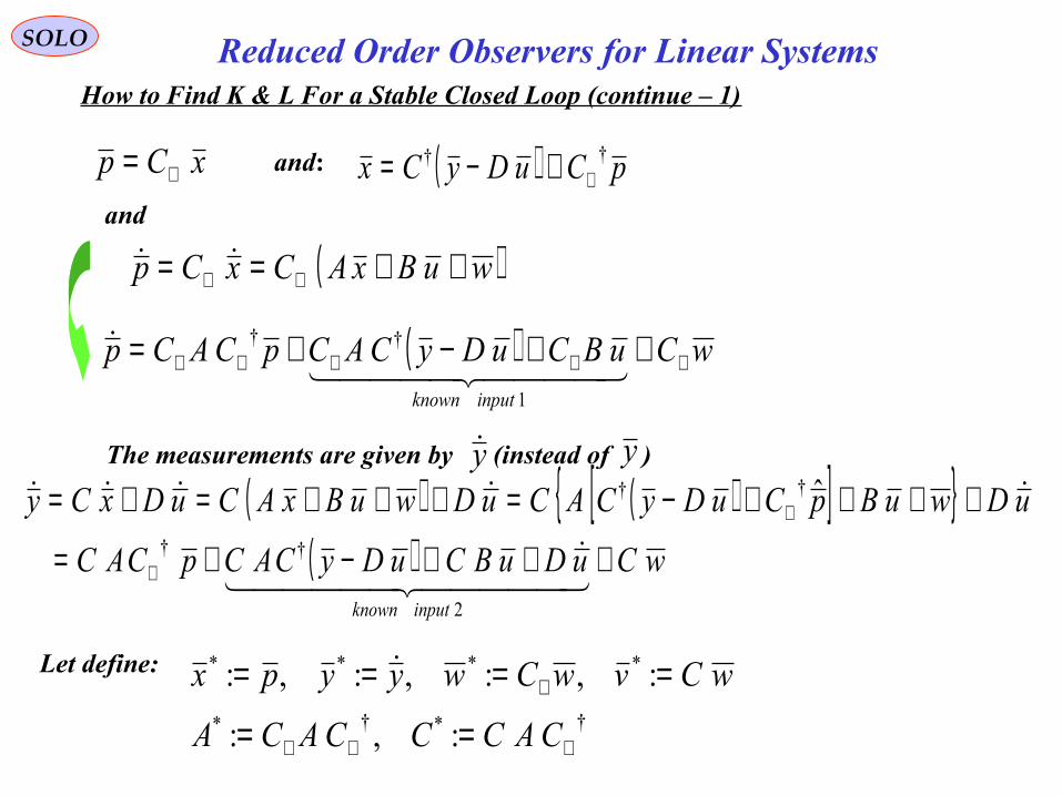
SOLO Reduced Order Observers for Linear SystemsHow to Find K & L For a Stable Closed Loop (continue – 1)
( ) wCuBCuDyCACpCACpinputknown
⊥⊥⊥⊥⊥ ++−+=
1
††
( ) pCuDyCx ††⊥+−=and:xCp ⊥=
and
( )wuBxACxCp ++== ⊥⊥
( ) ( )[ ]{ }( ) wCuDuBCuDyCACpCAC
uDwuBpCuDyCACuDwuBxACuDxCy
inputknown
+++−+=
++++−=+++=+=
⊥
⊥
2
††
†† ˆThe measurements are given by (instead of )y y
Let define:
†*†*
****
:,:
:,:,:,:
⊥⊥⊥
⊥
==
====
CACCCACA
wCvwCwyypx
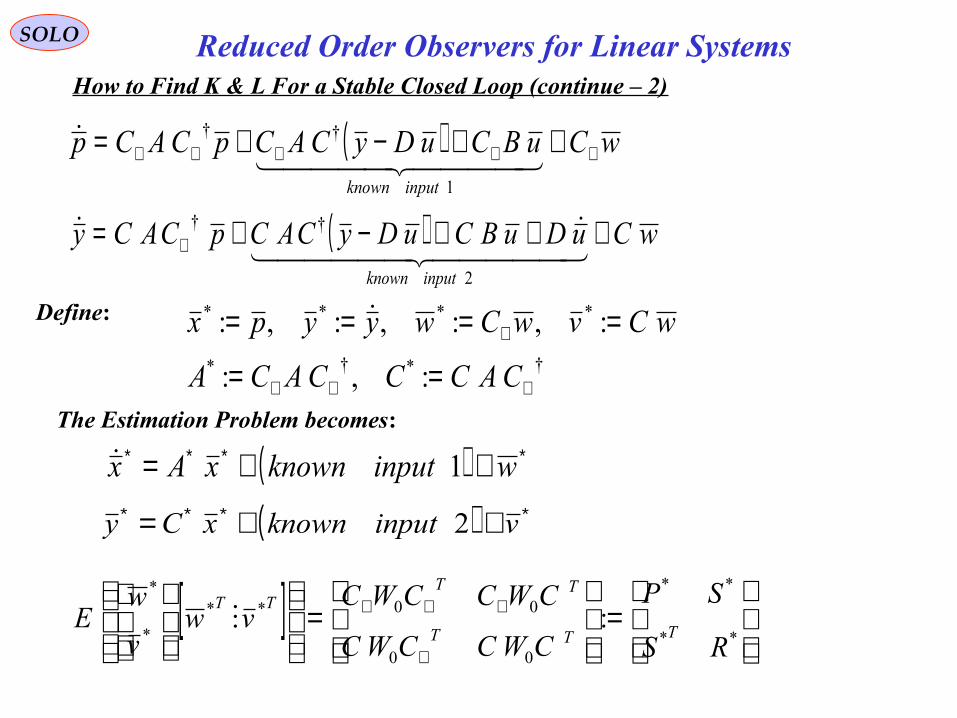
SOLO Reduced Order Observers for Linear SystemsHow to Find K & L For a Stable Closed Loop (continue – 2)
( ) wCuBCuDyCACpCACpinputknown
⊥⊥⊥⊥⊥ ++−+=
1
††
( ) wCuDuBCuDyCACpCACyinputknown
+++−+= ⊥
2
††
Define:
†*†*
****
:,:
:,:,:,:
⊥⊥⊥
⊥
==
====
CACCCACA
wCvwCwyypx
The Estimation Problem becomes:
( ) ∗∗∗∗ ++= winputknownxAx 1
( ) ∗∗∗∗ ++= vinputknownxCy 2
[ ]
=
=
⊥
⊥⊥⊥
**
**
00
00**
*
*
:RS
SP
CWCCWC
CWCCWCvw
v
wE
TTT
TTTT
SOLO Reduced Order Observers for Linear SystemsHow to Find K & L For a Stable Closed Loop (continue – 3)
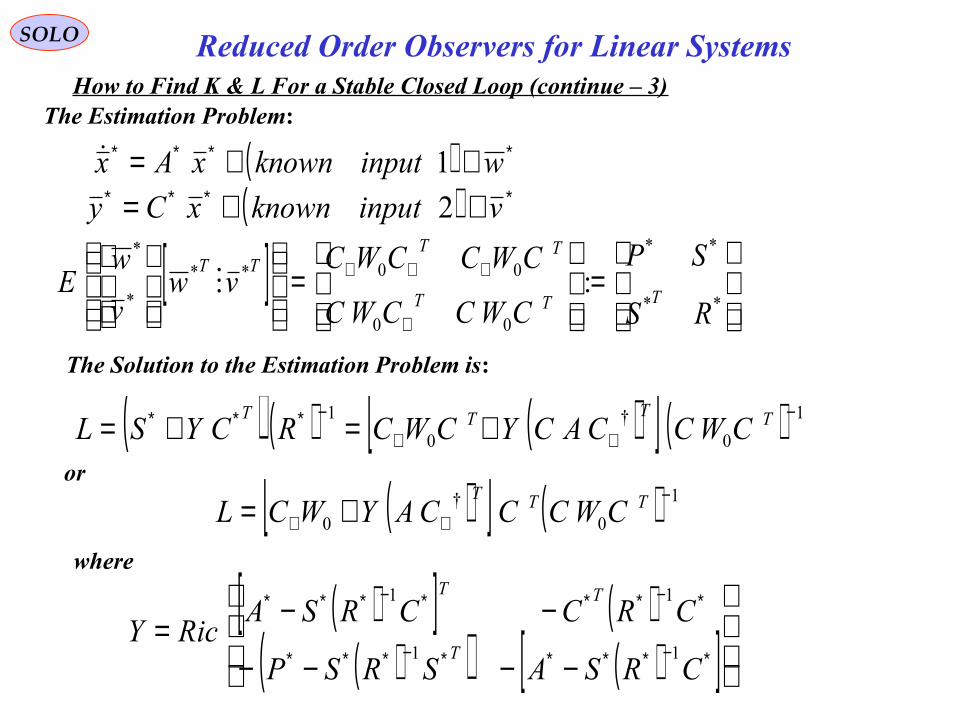
The Estimation Problem:
( ) ∗∗∗∗ ++= winputknownxAx 1
( ) ∗∗∗∗ ++= vinputknownxCy 2
[ ]
=
=
⊥
⊥⊥⊥
**
**
00
00**
*
*
:RS
SP
CWCCWC
CWCCWCvw
v
wE
TTT
TTTT
The Solution to the Estimation Problem is:
( ) ( ) ( )[ ] ( ) 10†
0
1 −⊥⊥
−∗∗∗ +=+= TTTTCWCCACYCWCRCYSL
or
( )[ ] ( ) 10†
0
−⊥⊥ += TTT
CWCCCAYWCL
where
( )[ ] ( )( )( ) ( )[ ]
−−−−
−−=∗−∗∗∗∗−∗∗∗
∗−∗∗∗−∗∗∗
CRSASRSP
CRCCRSARicY
T
TT
11
11
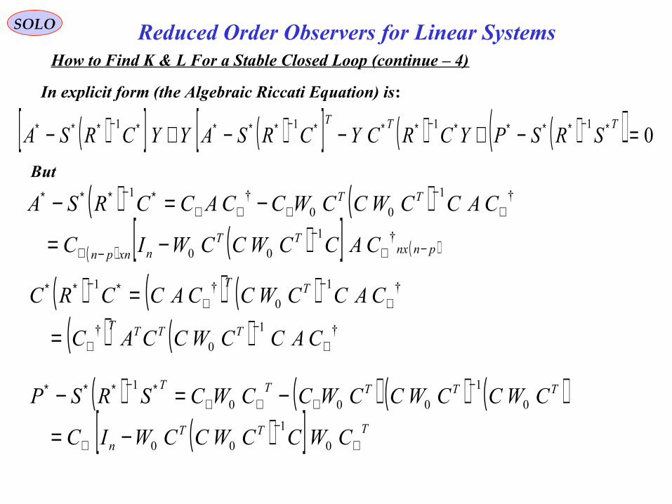
SOLO Reduced Order Observers for Linear SystemsHow to Find K & L For a Stable Closed Loop (continue – 4)
In explicit form (the Algebraic Riccati Equation) is:
But
( )[ ] ( )[ ] ( ) ( )( ) 01111 =−+−−+− ∗−∗∗∗∗−∗∗∗−∗∗∗∗−∗∗∗ TTT
SRSPYCRCYCRSAYYCRSA
( ) ( )( ) ( )[ ] ( )pnnx
TTnxnpn
TT
CACCWCCWIC
CACCWCCWCCACCRSA
−⊥−
−⊥
⊥−
⊥⊥⊥∗−∗∗∗
−=
−=−†1
00
†1
00†1
( ) ( ) ( )( ) ( ) †1
0†
†1
0†1
⊥−
⊥
⊥−
⊥∗−∗∗
=
=
CACCWCCAC
CACCWCCACCRC
TTTT
TT
( ) ( ) ( ) ( )( )[ ] TTT
n
TTTTT
CWCCWCCWIC
CWCCWCCWCCWCSRSP
⊥−
⊥
−⊥⊥⊥
∗−∗∗∗
−=
−=−
0
1
00
0
1
000
1
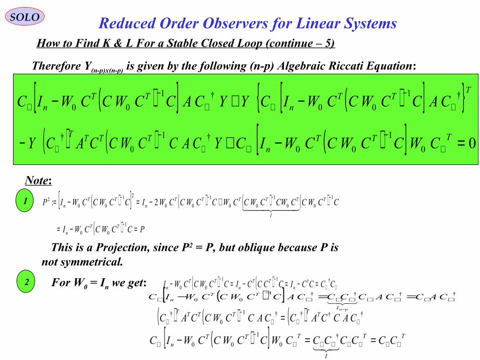
SOLO Reduced Order Observers for Linear SystemsHow to Find K & L For a Stable Closed Loop (continue – 5)
Therefore Y(n-p)x(n-p) is given by the following (n-p) Algebraic Riccati Equation:
( )[ ] ( )[ ]{ }TTTn
TTn CACCWCCWICYYCACCWCCWIC †1
00†1
00 ⊥−
⊥⊥−
⊥ −+−
( ) ( ) YCACCWCCACY TTTT †1
0†
⊥−
⊥− ( )[ ] 00
1
00 =−+ ⊥−
⊥TTT
n CWCCWCCWIC
Note:
1 ( )[ ] ( ) ( ) ( )
( ) PCCWCCWI
CCWCCCWCWCCWCCWCCWICCWCCWIP
TTn
T
I
TTTTTn
TTn
=−=
+−=−=
−
−−−−
1
00
1
00
1
00
1
00
21
002 2:
This is a Projection, since P2 = P, but oblique because P isnot symmetrical.
2 For W0 = In we get: ( ) ( ) ⊥⊥−−
=−=−=− CCCCICCCCICCWCCWI nTT
nTT
n††11
00
( ) ( ) ( ) ††††1
0†
⊥⊥⊥−
⊥ = CACCACCACCWCCAC TTTTTT
( )[ ] ††††1
00 ⊥⊥⊥⊥⊥⊥⊥−
⊥ ==−−
CACCACCCCACCWCCWIC
pnI
TTn
( )[ ] TT
I
TTTn CCCCCCCWCCWCCWIC ⊥⊥⊥⊥⊥⊥⊥
−⊥ ==−
†
0
1
00
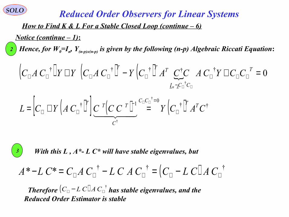
SOLO Reduced Order Observers for Linear SystemsHow to Find K & L For a Stable Closed Loop (continue – 6)
Hence, for W0=In, Y(n-p)x(n-p) is given by the following (n-p) Algebraic Riccati Equation:
Notice (continue – 1):
3 With this L , A*- L C* will have stable eigenvalues, but
2
( ) ( ) ( ) 0†††††
†
=+−+ ⊥⊥⊥−
⊥⊥⊥⊥⊥
⊥⊥
T
CCI
TTTCCYCACCACYCACYYCAC
n
( )[ ] ( ) ( ) ††0
1††
†
CACYCCCCAYCL TTCC
C
TTT
⊥
=−⊥⊥
⊥⊥
=+=
( ) †††** ⊥⊥⊥⊥⊥ −=−=− CACLCCACLCACCLA
Therefore has stable eigenvalues, and the Reduced Order Estimator is stable
( ) †⊥⊥ − CACLC
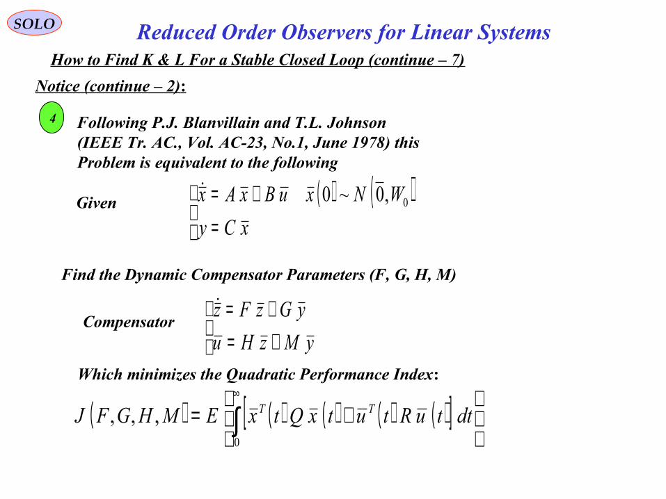
SOLO Reduced Order Observers for Linear SystemsHow to Find K & L For a Stable Closed Loop (continue – 7)
Notice (continue – 2):
4 Following P.J. Blanvillain and T.L. Johnson(IEEE Tr. AC., Vol. AC-23, No.1, June 1978) this Problem is equivalent to the following
( ) ( )
=+=xCy
WNxuBxAx 0,0~0Given
Find the Dynamic Compensator Parameters (F, G, H, M)
+=+=
yMzHu
yGzFzCompensator
Which minimizes the Quadratic Performance Index:
( ) ( ) ( ) ( ) ( )[ ]
+= ∫∞
0
,,, dttuRtutxQtxEMHGFJ TT
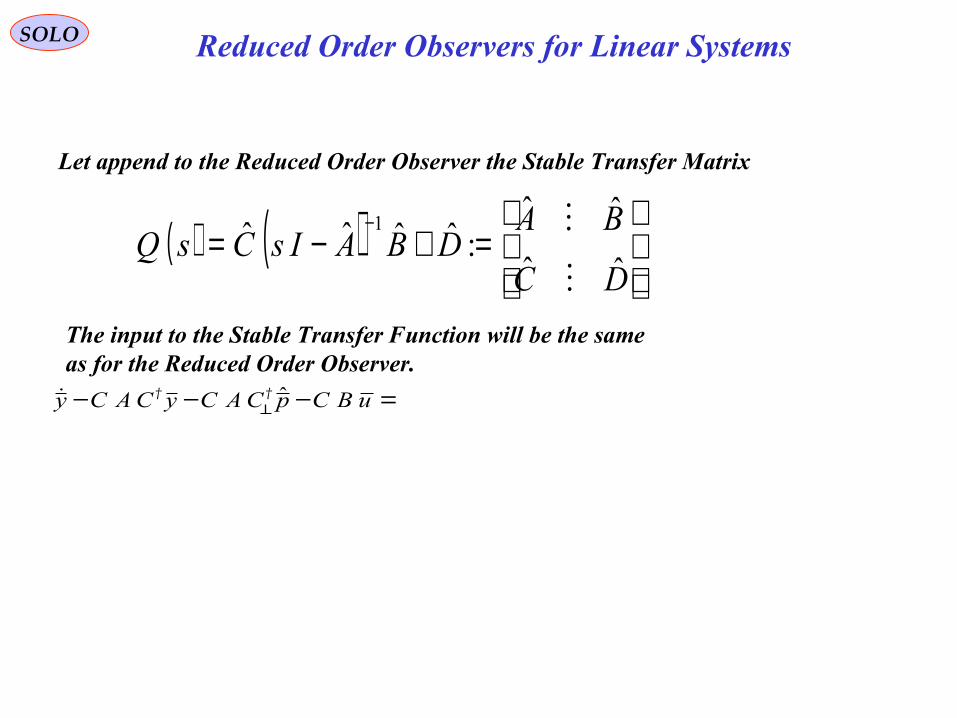
SOLO Reduced Order Observers for Linear Systems
Let append to the Reduced Order Observer the Stable Transfer Matrix
( ) ( )
=+−=
−
DC
BADBAIsCsQ
ˆˆ
ˆˆ:ˆˆˆˆ 1
=−−− uBCpCACyCACy ˆ††
The input to the Stable Transfer Function will be the same as for the Reduced Order Observer.
References
SOLO
Kwakernaak, H., Sivan, R., “Linear Optimal Control Systems”, Wiley Inter-science, 1972, pg.335
Reduced Order Observers for Linear Systems
Gelb A. Ed, “Applied Optimal Estimation”, The Analytic Science Corporation, 1974, pg.320

August 13, 2015 30
SOLO
TechnionIsraeli Institute of Technology
1964 – 1968 BSc EE1968 – 1971 MSc EE
Israeli Air Force1970 – 1974
RAFAELIsraeli Armament Development Authority
1974 –2013
Stanford University1983 – 1986 PhD AA