Reduced-order description of transient instabilities and computationof finite-time Lyapunov exponents

Hessam Babaee,1,2 Mohamad Farazmand,1 George Haller,3 and Themistoklis P. Sapsis1,a)

1Department of Mechanical Engineering, MIT Cambridge, Cambridge, Massachusetts 02139, USA2Department of Mechanical Engineering and Materials Science, University of Pittsburgh, Pittsburgh,Pennsylvania 15261, USA3Department of Mechanical and Process Engineering, ETH Zurich, 8092 Zurich, Switzerland

(Received 28 January 2017; accepted 1 May 2017; published online 6 June 2017)

High-dimensional chaotic dynamical systems can exhibit strongly transient features. These areoften associated with instabilities that have a finite-time duration. Because of the finite-time charac-ter of these transient events, their detection through infinite-time methods, e.g., long term averages,Lyapunov exponents or information about the statistical steady-state, is not possible. Here, we uti-lize a recently developed framework, the Optimally Time-Dependent (OTD) modes, to extract atime-dependent subspace that spans the modes associated with transient features associated withfinite-time instabilities. As the main result, we prove that the OTD modes, under appropriate condi-tions, converge exponentially fast to the eigendirections of the Cauchy–Green tensor associatedwith the most intense finite-time instabilities. Based on this observation, we develop a reduced-order method for the computation of finite-time Lyapunov exponents (FTLE) and vectors. In high-dimensional systems, the computational cost of the reduced-order method is orders of magnitudelower than the full FTLE computation. We demonstrate the validity of the theoretical findings ontwo numerical examples. Published by AIP Publishing. [http://dx.doi.org/10.1063/1.4984627]

For a plethora of dynamical systems transient phenom-ena—usually associated with finite-time instabilities—define the most important aspects of the response.Examples include rare chaotic bursts in turbulent sys-tems, extreme events in nonlinear waves, and strong tran-sients in complex networks. In such systems, the raretransient responses coexist with a high dimensional cha-otic attractor where the system spends most of its lifetime.Because of the rare character of the transient dynamics, itis particularly challenging to extract modes that capturethem using traditional methods for order reduction andbase selection. Here, we prove that a recently developedmethod, the optimally time-dependent (OTD) modes, pro-vides a time-dependent basis that spans the directionsassociated with the most intense instabilities, even if thesehave short-time character. Therefore, the derived modesencode the strongly time-dependent features of the associ-ated instabilities. We demonstrate the developed frame-work through the computation of finite-time Lyapunovexponents (FTLE) utilizing only the projected dynamicsalong the derived modes.

I. INTRODUCTION

For a plethora of dynamical systems transient phenom-ena—usually associated with finite-time instabilities—definethe most important aspects of the response. Examples includechaotic fluid systems,4,16,17 nonlinear waves,8,9 and net-works.7,38 For the analysis of such systems and the formulation

of prediction and control algorithms, it is critical to identifymodes associated with these strongly transient features. A firstimportant challenge towards identifying these modes is thehigh-dimensionality of the response. This high-dimensionalitydoes not necessarily imply that the transient features are alsohigh-dimensional. In fact, it is often the case that the modesassociated with transient features are very few. However,because of the broad spectrum of the response it is hard toidentify them using energy-based criteria. An additional chal-lenge is associated with the intrinsically time-dependent char-acter of these features which is, in general, non-periodic andmakes it essential to consider arbitrary time-dependence forthese modes as well.

In the context of dynamical systems, numerousapproaches have been developed to characterize the transientfeatures associated with non-periodic behavior. The notion ofLagrangian Coherent Structures (LCS) emerged from thefluid dynamics problem of mixing as a general method tocharacterize dynamical systems with arbitrary time-depen-dence.20,22,26 The method quantifies finite-time instabilitiesthrough the explicit computation of the maximum eigenvalueof the Cauchy–Green tensor on every location of the phasespace. For low-dimensional systems, it provides a completeand unambiguous description of the finite-time instabilitiesby identifying parts of the phase space associated with suchresponses. However, given the fast growth of the computa-tional cost with respect to the phase space dimensionality it isnot possible to apply it for very high- or infinite-dimensionalsystems in order to characterize finite-time instabilities.

For such problems, other approaches focusing more onthe description of the system attractor rather than the wholephase space have also been developed in the context of

a)Author to whom correspondence should be addressed: sapsis@mit.edu.Tel.: (617) 324-7508. Fax: (617) 253-8689.

1054-1500/2017/27(6)/063103/12/$30.00 Published by AIP Publishing.27, 063103-1

CHAOS 27, 063103 (2017)

uncertainty quantification and model order reduction.Specifically, the notion of dynamical orthogonality5,6,33,34

allows for the computation of time-dependent, dynamicallyorthogonal (DO) modes that lead to reduced-order descrip-tion of chaotic attractors with low-intrinsic dimensionalitybut with strong time-dependence.31,32 The same notion canbe combined with stochastic closures35,37 in order to quantifystatistics in time-dependent subspaces for turbulent dynamicssystems with very broad spectra (or high intrinsic dimension-ality) and strongly transient features.27,36 In all of these stud-ies, the effectiveness of the derived DO modes in capturingtransient responses was demonstrated numerically and veryfew theoretical studies related to this problem were con-strained in very specific setups. One such case is the study oflinear parabolic (stable) equations in Ref. 28 where it wasshown that the DO modes tend to capture the most energeticdirections. However, there is no general result indicatingwhere the DO modes converge for an arbitrary (nonlinear)dynamical system.

To circumvent this limitation, a minimization principlewas introduced in Ref. 2 that allows for the derivation ofequations that evolve a time-dependent set of modes, theOptimally Time Dependent (OTD) modes, along a given tra-jectory of the system. These modes are identical to thoseobtained from the DO equations in the deterministic limit,i.e., for the case where the stochastic energy goes to zero. Tothis end, the OTD modes can be seen as the deterministicanalog of DO modes. For sufficiently long times where thesystem reaches an equilibrium, it was proven in Ref. 2 thatthe OTD modes converge to the most unstable directions ofthe system in the asymptotic limit. Moreover, the samemodes were utilized in Ref. 16 to formulate predictors ofextreme events for Navier-Stokes equations and nonlinearwave problems.

Despite their success in numerically capturing transientphenomena associated with finite-time instabilities, the exactrelation between OTD modes (or DO modes) and finite-timeinstabilities remains an open problem. In this work, we pro-vide a rigorous link between the OTD modes and finite-timeinstabilities, by showing that under general conditions theOTD modes converge exponentially fast to the eigendirec-tions of the Cauchy–Green tensor associated with the largesteigenvalues, i.e., with the largest finite-time Lyapunov expo-nents. Thus, we prove that the OTD modes are able to extractover a finite-time interval the modes associated with themost intense finite-time instabilities or the most pronouncedtransient phenomena. Note, that such convergence does notdepend on the dimensionality of the system or the intrinsicdimensionality of the attractor.

Apart from the fundamental implications of this result onthe formulation of reduced-order algorithms for the predic-tion and control of transient phenomena, there is a directapplication on the computation of the maximum finite-timeLyapunov exponents for high- or infinite-dimensional sys-tems. Specifically, using the OTD modes we formulate areduced-order framework that allows, under mild conditions,the computation of finite-time Lyapunov Exponents for gen-eral dynamical systems without having to compute the fullCauchy–Green tensor. We demonstrate the derived algorithm

in two systems, the Arnold-Beltrami-Childress (ABC) flowand the Six-dimensional Charney-DeVore (CDV) model withregime transitions. In both cases, we examine the effective-ness of the reduced-order method and study limitations andapplicability.

II. PRELIMINARIES AND NOTATION

We consider the system of differential equations

_z ¼ f ðz; tÞ; z 2 Rn; t 2 I ¼ t0; t0 þ T½ &; (1)

where f : U ' I ! Rn is a sufficiently smooth vector field.Let Ft

t0with t 2 I denote the associated flow map,

Ftt0

: U ! U

z0 7! zðt; t0; z0Þ; (2)

where zðt; t0; z0Þ is a trajectory of system (1) with the initialcondition z0. The linearized system around the trajectoryzðtÞ ( zðt; t0; z0Þ satisfies the equation of variations,

_v ¼ LðzðtÞ; tÞv; vðtÞ 2 Rn; t 2 I ¼ t0; t0 þ T½ &; (3)

where Lðz; tÞ :¼ rzf ðz; tÞ. The deformation gradient rFtt0

isthe fundamental solution matrix for the linearized dynamicssuch that the solutions vðtÞ ( vðt; t0; v0Þ of the equation ofvariations satisfy

vðt; t0; z0Þ ¼ rFtt0ðz0Þv0; with t 2 I ¼ t0; t0 þ T½ &: (4)

A. Finite-time Lyapunov exponents

To measure the growth of infinitesimal perturbations inthe phase space, we use the right Cauchy–Green straintensor

Ctt0¼ ðrFt

t0ÞTrFt

t0;

and the left Cauchy–Green strain tensor

Btt0¼ rFt

t0ðrFt

t0ÞT ; (5)

where T denotes matrix transposition. Let nðt; t0; z0Þ 2 Rn

denote the eigenvectors of the right Cauchy–Green straintensor, so that

Ctt0ðz0Þniðt; t0; z0Þ ¼ kiðt; t0; z0Þniðt; t0; z0Þ; i ¼ 1;…; n;

where kiðt; t0; z0Þ are the corresponding eigenvalues.Similarly, denote the eigenvectors of the left Cauchy–Greenstrain tensor by giðt; t0; z0Þ 2 Rn and their correspondingeigenvalues by liðt; t0; z0Þ, so that

Btt0ðz0Þgiðt; t0; z0Þ ¼ liðt; t0; z0Þgiðt; t0; z0Þ; i ¼ 1;…; n:

When no confusion may arise, we omit the dependence ofthe eigenvalues and eigenvectors on ðt; t0; z0Þ for notationalsimplicity. Since the Cauchy–Green strain tensors are sym-metric and positive definite, their eigenvalues are real and

063103-2 Babaee et al. Chaos 27, 063103 (2017)

positive, ki; li 2 Rþ. Furthermore, the eigenvectors areorthogonal, i.e.,

hni; nji ¼ hgi; gji ¼ dij; i; j ¼ 1;…; n;

where h); )i denotes the Euclidean inner product.It is straightforward to show that the right and left ten-

sors have the same eigenvalues, ki ¼ li. Specifically, consid-ering the definition of the right Cauchy–Green tensoreigenvalues, ðrFt

t0ÞTrFt

t0ni ¼ kini, we multiply the equation

with rFtt0

from the left to obtain

Btt0ðrFt

t0niÞ ¼ kiðrFt

t0niÞ: (6)

Thus, the left and right Cauchy–Green strain tensors havethe same set of eigenvalues. Finally, using the singular valuedecomposition of the deformation gradient, one can showthe well-known relation that

rFtt0ni ¼

ffiffiffiffiki

pgi; i ¼ 1;…; n; (7)

(see, e.g., Ref. 23). In the following, we order theCauchy–Green eigenvalues in a descending order,

k1 > k2 > ) ) ) > kn > 0: (8)

The finite-time Lyapunov exponents (FTLEs) of system (1)corresponding to the trajectory zðt; t0; z0Þ and the time inter-val ½t0; t0 þ T& are defined as

Ki t0 þ T; t0; z0ð Þ ¼1

Tlog

ffiffiffiffiffiffiffiffiffiffiffiffiffiffiffiffiffiffiffiffiffiffiffiffiffiffiffiffiffiffiffiki t0 þ T; t0; z0ð Þ

p;

i ¼ 1; 2;…; n:(9)

Note that FTLEs are well-defined for any finite integra-tion time T. Under certain assumptions, the limit T !1also exists.30

B. Optimally time-dependent (OTD) modes

We give an overview of the OTD modes2 for generaldynamical systems. The OTD modes represent a reduced-order set of r time-dependent orthonormal modes, UðtÞ¼ ½u1ðtÞ; u2ðtÞ;…; urðtÞ&, that minimize the differencebetween the action of the infinitesimal propagator rFtþdt

t onuiðtÞ and its value at time tþ dt. More specifically, we seekto minimize the functional

F ¼ 1

dtð Þ2Xr

i¼1

jjui tþ dtð Þ *rFtþdtt ui tð Þjj2; dt! 0; (10)

with the constraint that the time-dependent basis satisfies theorthonormality conditions

huiðtÞ; ujðtÞi ¼ dij; i; j ¼ 1;…; r: (11)

Using Taylor series expansions, we have

uiðtþ dtÞ ¼ uiðtÞ þ dt _ui þOðdt2Þ; (12)

rFtþdtt ¼ I þ dt LðzðtÞ; tÞ þOðdt2Þ; (13)

where I is the identity matrix. Replacing the above equationsinto the functional (10) results in

F _u1; _u2;…; _urð Þ ¼Xr

i¼1

""""@ui tð Þ@t* L z tð Þ; tð Þui tð Þ

""""2

: (14)

We emphasize that the minimization of the function(14) is considered only with respect to the time-derivative(rate of change) of the basis, _UðtÞ; instead of the basis U(t)itself. This is because we do not want to optimize the sub-space that the operator is acting on, but rather find an optimalset of vectors, _UðtÞ; that best approximates the linearizeddynamics in the subspace U. We then solve the resultedequations and compute U(t). We will refer to these modes asthe optimally time-dependent (OTD) modes, and the spacethat these modes span as the OTD subspace. By utilizing theminimization principle and taking into account the orthonor-mality constraint, we obtain the following theorem (provedin Ref. 2.)

Theorem 2.1. A one parameter family of vectorsuiðtÞ 2 Rn; i ¼ 1; 2;…; r, minimizes the functional (14) andsatisfies the orthonormality condition (11) if and only if

@U

@t¼ LU * UUT LU; (15)

where U tð Þ ¼ u1 tð Þ; u2 tð Þ;…; ur tð Þ½ & 2 Rn'r:Equation (15) is the evolution equation for the OTD

modes. It was proven in Ref. 2 that for the case of a timeindependent operator, L, the subspace spanned by the col-umns of U(t) converges asymptotically to the modes associ-ated with the most unstable directions of the operator L.

The OTD modes were also used to capture the transientnon-normal growth of instabilities. In Fig. 1, we recall a sys-tem from Ref. 2 exhibiting a non-normal growth (cf. Ref. 2for the details). A typical trajectory of the system, shown inthe left panel, has an almost periodic behavior where eachcycle exhibits three distinct regimes: (A) an exponentialgrowth in the z3 direction, (B) a non-normal growth in thez1 * z2 plane with simultaneous decay in the z3 direction, and(C) exponential decay in the z1 * z2 plane to the origin. Thisconfiguration allows for the repeated occurrence of exponen-tial (regime A) and non-normal (regime B) instabilities.

Due to the exponential instability close to the origin, thesystem undergoes chaotic transitions between positive andnegative values of z3. We compute the instantaneous growthrate corresponding to the direction of a single OTD mode.The OTD mode initially captures the severe exponentialgrowth and subsequently captures the non-normal growth. Onthe other hand, the real part of the eigenvalues of the full line-arized operator can only capture the exponential growth, evenin regimes where it is not relevant, while they completelymiss the non-normal growth. The maximum largest singularvalue r of the matrix L exhibits a similar behavior.

The OTD modes share some fundamental characteristicsof other stability measures. In Sec. III, we show the relationbetween the OTD modes and the finite-time Lyapunovvectors. In Appendix A, we also discuss the connectionbetween them and the Dynamically Orthogonal (DO) modes

063103-3 Babaee et al. Chaos 27, 063103 (2017)

introduced in Ref. 33. Their connection with covariantLyapunov vectors18 remains to be explored.

III. ALIGNMENT OF THE OTD MODES WITH THEDOMINANT CAUCHY–GREEN STRAINEIGENVECTORS

Here, we prove that under proper assumptions, the OTDmodes not only capture the unstable directions of steady lin-ear operators, but also the transient instabilities associatedwith time-dependent operators. More specifically, we provethat the OTD subspace converges exponentially fast to theeigenspace associated with the dominant eigenvalues of theCauchy–Green strain tensor. The latter describes the finite-time growth of infinitesimal perturbations in the phase space.For what follows, we will need to measure the distancebetween two subspaces of the same dimensionality. To thisend, we need the following definitions.

Definition 3.1. Two r-dimensional linear subspaces ofRn spanned by the columns of U 2 Rn'r and V 2 Rn'r areequivalent if there is an invertible matrix R 2 Rr'r such thatU¼VR.

The next definition provides a quantity for measuringthe “angle” between two subspaces.

Definition 3.2. For two r-dimensional linear subspacesof Rn spanned by the columns of U ¼ ½u1; u2;…; ur& 2 Rn'r

and V ¼ ½v1; v2;…; vr& 2 Rn'r, we define the distancefunction

cU;V ¼jjUTVjj

r1=2; (16)

where jj ) jj denotes the Frobenius norm.Note that the entries of UTV are the inner products

between ui’s and vj’s, i.e., ðUTVÞij ¼ hui; vji. The followinglemma shows that the equivalence of two subspaces can bededuced from the distance cU;V .

Lemma 3.1. Given a subspace defined by the orthonor-mal columns of U 2 Rn'r, and a subspace defined by theunit-length (but not necessarily orthonormal) columns ofV 2 Rn'r, then we always have cU;V + 1. Moreover, the twosubspaces spanned by the columns of U and V are equivalentif and only if cU;V ¼ 1.

Proof. By the orthogonal projection theorem, there arehi 2 Rr and bi 2 Rn such that vi ¼ Uhi þ bi and UTbi ¼ 0for i ¼ 1; 2;…; r. Note that since vi are unit length, we have

1 ¼ jjvijj2 ¼ jjhijj2 þ jjbijj2; i ¼ 1; 2;…; r:

Defining H ¼ ½h1j ) ) ) jhr& and B ¼ ½b1j ) ) ) jbr&, we haveV ¼ UH þ B. This implies UTV ¼ H and hence

jjUTVjj2 ¼ jjHjj2 ¼Xr

i¼1

jjhijj2 ¼ r *Xr

i¼1

jjbijj2 ¼ r * jjBjj2:

Therefore, c2U;V ¼ 1* jjBjj2=r. Note that the subspaces colðUÞ

and colðVÞ are equal if and only if jjBjj ¼ 0. Therefore,colðUÞ ¼ colðVÞ if and only if cU;V ¼ 1. We also note that ifthe two subspaces are not equivalent cU;V < 1: !

To prove the main theorem, it is more convenient towork with the subspace spanned by the linearized flow (3),instead of the OTD subspace. The following result states thatthe two subspaces are equivalent.

Theorem 3.1. Let VðtÞ 2 Rn'r solve the equation ofvariations (3) and UðtÞ 2 Rn'r with UTU ¼ I solve the OTDequation (15). Assume that the two subspaces spanned by thecolumns of U and V are initially equivalent, i.e., there is aninvertible matrix T0 2 Rr'r such that V0 ¼ U0T0. Then,there exists a one-parameter family of linear transformationsT(t) such that VðtÞ ¼ UðtÞTðtÞ for all t and T(t) satisfies thedifferential equation

_T ¼ LrðtÞT; Tðt0Þ ¼ T0; (17)

where Lr ¼ UTLU is the orthogonal projection of L to thelinear subspace spanned by the columns of U.

Proof. See Theorem 2.4 in Ref. 2. !Based on this equivalence, it is sufficient to study the

behavior of the subspace evolved under the time-dependentlinearized dynamics (3) in order to understand the propertiesof the OTD subspace. Specifically, we use this lemma toprove the main result of this paper, namely, that under aspectral gap condition, the OTD subspace will converge tothe dominant directions of the Cauchy–Green strain tensor.

Theorem 3.2. Let niðt; t0; z0Þ and giðt; t0; z0Þ ði ¼ 1;2;…; nÞ denote the eigenvectors of the right and leftCauchy–Green strain tensors, respectively, with correspond-ing eigenvalues k1ðt; t0;z0Þ , k2ðt; t0;z0Þ , ) ) ) , knðt; t0; z0Þ.Moreover, let UðtÞ 2Rn'r solve the OTD equation (15)along the trajectory zðt; t0;z0Þ. Assume that

(i) The subspace U(t) is initiated so that each basis elementuiðt0Þ has a non-zero projection on at least one of theeigenvectors niðt; t0; z0Þ; i ¼ 1; 2;…; r for all times t.

FIG. 1. An example of the OTD modeson the analysis of transient instabil-ities. Left: A trajectory of the dynami-cal system colored according to thestate variable z3. The non-normal vec-tor field for z3 ¼ 0 is also shown.Right: The three eigenvalues of the lin-earized operator are plotted with bluedashed curves, while the growth rate ofthe single OTD mode is shown withorange color. The maximum eigen-value of the singular value decomposi-tion of the linearization along thetrajectory is also shown.

063103-4 Babaee et al. Chaos 27, 063103 (2017)

(ii) The trajectory zðt; t0; z0Þ is hyperbolic in the sense thatthere exist constants a1 , a2 , ) ) ) , ar > arþ1 ,) ) ) , an and Ki > 0 ði ¼ 1; 2;…; nÞ such that

limt!1

ki t; t0; z0ð Þeait

¼ Ki: (18)

Then, the subspace U(t) aligns with the r most domi-nant left Cauchy–Green strain eigenvectors, giðt; t0;z0Þ; i ¼ 1;…; r, exponentially fast as t!1.

Proof. Based on Lemma 3.1 the subspace spanned bythe OTD modes is equivalent to the subspace that we obtainif we evolve VðtÞ ¼ ½v1ðtÞ;…; vrðtÞ& using the linearizeddynamics (3). We represent the initial condition for theequation of variations (3) as Vðt0Þ ¼ ½v01

; v02;…; v0r & and

express it in terms of the orthonormal strain eigenbasisfniðt; t0; z0Þg as

v0j ¼Xn

i¼1

hv0j ; niðt; t0; z0Þiniðt; t0; z0Þ; j ¼ 1;…; r: (19)

Then, Eqs. (4) and (7) applied to Eq. (19) yield

vjðt; t0; z0Þ ¼Xn

i¼1

ffiffiffiffiffiffiffiffiffiffiffiffiffiffiffiffiffiffiffiffikiðt; t0; z0Þ

phv0j ; niðt; t0; z0Þigiðt; t0; z0Þ;

j ¼ 1;…; r:

We then have

hvjðt; t0; z0Þ; gkðt; t0; z0Þi ¼ffiffiffiffiffiffiffiffiffiffiffiffiffiffiffiffiffiffiffiffiffikkðt; t0; z0Þ

phv0j ; nkðt; t0; z0Þi;

j; k ¼ 1;…; r:

Moreover,

hvjðt; t0; z0Þ; vjðt; t0; z0Þi ¼Xn

i¼1

kiðt; t0; z0Þhv0j ; niðt; t0; z0Þi2;

j ¼ 1;…; r:

Based on this last equation, the cosine of the angleavj;gkðt; t0; z0Þ between the vector vjðt; t0; z0Þ and the eigen-

vector gkðt; t0; z0Þ of Btt0ðz0Þ obeys the relation

cos avj;gk¼hvj t; t0; z0ð Þ; gkijjvj t; t0; z0ð Þjj

¼ffiffiffiffiffikkphv0j ; nkiffiffiffiffiffiffiffiffiffiffiffiffiffiffiffiffiffiffiffiffiffiffiffiffiffiffiffiffiffiffiffiffiPn

i¼1 kihv0j ; nii2q : (20)

Identity (20) and Definition 3.2 yield

rc2v;g ¼

Xr

j¼1

Xr

k¼1

kkhv0j ; nki2Pni¼1 kihv0j ; nii2

¼Xr

j¼1

Prk¼1 kkhv0j ; nki2Pni¼1 kihv0j ; nii2

¼Xr

j¼1

Aj

Aj þ Bj: (21)

where

Aj ¼Xr

k¼1

kkhv0j ; nki2 , kr

Xr

k¼1

hv0j ; nki2;

Bj ¼Xn

i¼1

kihv0j ; nii2 + krþ1

Xn

i¼rþ1

:hv0j ; nii2

Note that assumption (ii) implies limt!1 krþ1ðt; t0; z0Þ=krðt; t0; z0Þ ¼ 0 since

limt!1

krþ1 t; t0; z0ð Þkr t; t0; z0ð Þ

¼ limt!1

krþ1 t; t0; z0ð Þ=earþ1t

kr t; t0; z0ð Þ=eart

earþ1t

eart;

¼ Krþ1

Krlimt!1

e arþ1*arð Þt:

As a consequence, we obtain from the last inequality theestimate

rc2v;g ¼

Xr

j¼1

1

1þBj

Aj

,Xr

j¼1

1

1þ krþ1

kr

Pni¼rþ1 hv0j ; nii2Prk¼1 hv0j ; nki2

:

(22)

Note thatPr

k¼1 hv0j ; nki2 > 0 from the first assumption.Therefore, for the asymptotic limit t!1, we have

c2v;g , 1:

Note that the way we have defined the two subspaces satisfythe assumptions of Lemma 3.1 and therefore we always havec2v;g + 1. Thus, c2

v;g ¼ 1 which implies that the two subspacesare equivalent. This completes the proof. !

We point out that the hyperbolicity condition (ii) is not anecessary condition. In fact, as long as the ratio krþ1ðtÞ=krðtÞtends to zero asymptotically, the alignment takes place [seeEq. (22)].

IV. EIGENVALUE CROSSING AND OTD MODES

Theorem 3.2 shows that under appropriate assumptionsthe OTD modes converge exponentially fast to the eigen-space of the left Cauchy–Green strain tensor associated withthe largest Lyapunov exponents. This convergence, however,may be interrupted when the smallest eigenvalue spanned bythe OTD modes crosses with the one that is not beingspanned. In Fig. 2, we illustrate this situation. The green

FIG. 2. Evolution of the principal eigenvector (red) of the Cauchy–Greentensor. When eigenvalue crossing occurs, the rate of change becomesunbounded. This is not a problem if all the eigenvectors are resolved but it isimportant if we evolve only the dominant eigenvectors as it is the case withthe OTD modes.

063103-5 Babaee et al. Chaos 27, 063103 (2017)

curve denotes the trajectory of the system, while the ellipsesindicate the principal axes of the left Cauchy–Green straintensor. Assuming that we are resolving only one OTD mode,after sufficient time this must have converged to the correctprincipal direction (red arrow). As we go through the criticaltime instant where the ellipsoid becomes a circle due toeigenvalue crossing, we observe that the principal directionsare instantaneously ill-defined. Immediately after the eigen-value crossing, the dominant principal direction undergoesa 90- internal rotation compared to immediately beforethe crossing. The OTD modes, on the other hand, evolvesmoothly and are unable to capture such an instantaneouslyunbounded transition.

In the context of shearless Lagrangian coherent struc-tures, these eigenvalue crossings are referred to as theCauchy–Green singularities and play an important role inthe computation of jet cores.12 In a more general application,the significance of these singularities is pointed out byLancaster24 who derived the rate of change of the eigenvec-tors of an arbitrary symmetric matrix, proving the followingtheorem.

Theorem 4.1. The rate of change of the eigenvectorsRðtÞ 2 Rn'n of a symmetric matrix GðtÞ 2 Rn'n is describedby the equation

_R ¼ RK; (23)

where K(t) is a skew-symmetric matrix given by

Kij tð Þ ¼~Gij tð Þ þ ~Gji tð Þ

2 kj tð Þ * ki tð Þ# $ ; i 6¼ j; (24)

with ~GðtÞ ¼ RTðtÞ _GðtÞRðtÞ and kiðtÞ being the eigenvalues ofG(t).

Proof. See Appendix B or Ref. 24. !As ki approaches kj, _R becomes unbounded, consistent

with the description given previously. This is not a problemif both of the eigen-directions corresponding to ki and kj arebeing spanned/resolved by the OTD subspace. The corre-sponding OTD subspace will just evolve smoothly in thiscase. However, if the eigenvalue crossing occurs with aneigendirection that is not being spanned by the OTD sub-space, the latter will have to instantaneously “steer” towardsa direction that is orthogonal to it.

This is not possible since it can be easily seen that forany bounded operator L, the rate of change of the corre-sponding OTD modes [Eq. (15)] is bounded

_U ¼ QLU ) jj _U jj + jjQjjjjLjjjjUjj; (25)

where Q is a projection operator (therefore bounded) and Uis also bounded. If the eigenvalue crossing involves modesalready contained in U, then there is no need for infiniterate of change of the modes, because existing modes justexchange roles (or indices). However, if there is eigen-value crossing between a mode that is contained in Uand another one that is not contained then it is essential tohave an evolution of the direction in U to an orthogonaldirection (not contained in U) and this cannot happeninstantaneously.

Therefore, we see that the convergence of the OTDmodes can be compromised if there are eigenvalue crossingsinvolving directions not spanned by the OTD subspace. Notehowever that such eigenvalue crossing will only influencethe convergence of the OTD mode associated with the small-est finite-time Lyapunov exponent captured within the OTDsubspace. Assuming that there are no subsequent eigenvaluecrossings with larger eigenvalues, one expects that the OTDsubspace would capture the directions associated with thelargest finite-time Lyapunov exponents.

Thus, for systems where eigenvalue crossing occurs, alarger OTD subspace guarantees that the principal axes asso-ciated with the largest Lyapunov exponents will be capturedby the OTD modes. Note that such convergence does notdepend on the physical dimension of the system or the intrin-sic dimension of the underlying attractor. This is particularlyimportant for systems where instabilities of isolated modesemerge out of high-dimensional stochastic backgrounds, suchas intermittent dissipation bursts in turbulence16 or focusinginstabilities occurring in nonlinear stochastic waves.9,16

As we demonstrate in Sec. V, for many practical appli-cations, it is sufficient to compute just the maximum finite-time Lyapunov exponent so what is important is to have themost dominant direction of the Cauchy–Green tensor cap-tured by the OTD subspace. The benefits of such an approachare, of course, more important as the dimension n of theunderlying system increases.

V. REDUCED-ORDER COMPUTATION OF FINITE-TIMELYAPUNOV EXPONENTS

As shown above, the OTD modes are able to extract thetransiently most unstable directions independent of theattractor dimensionality. Consequently, the OTD basis canbe used for the reduced-order approximation of finite-timeLyapunov exponents (FLTE) of high-dimensional systems.Specifically, we apply the following approximation schemefor the computation of a FTLE corresponding to a time inter-val of length T.

(1) Advect the trajectory zðt; t0; z0Þ for an interval t 2½t0; t0 þ T& where z0 is the initial point.

(2) Compute the r-dimensional OTD subspace U(t) corre-sponding to this trajectory.

(3) Compute the low-dimensional fundamental solutionmatrix Ut

t02 Rr'r using the reduced linear dynamical

system

d

dtUt

t0¼ Lr z tð Þ; tð ÞUt

t0; Ut0

t0¼ I; t 2 t0; t0 þ T½ &; (26)

where Lrðz; tÞ ¼ UðtÞTLðz; tÞUðtÞ is the projection of thefull linearized operator L onto the OTD subspace, whichcontains the most unstable directions.

(4) Compute the reduced-order finite-time Lyapunovexponents,

Ci t0 þ T; t0; z0ð Þ ¼1

Tlog

ffiffiffiffiffiffiffiffiffiffiffiffiffiffiffiffiffiffiffiffiffiffiffiffiffiffiffiffiffiffiffici t0 þ T; t0; z0ð Þ

p; i ¼ 1;…; r;

(27)

063103-6 Babaee et al. Chaos 27, 063103 (2017)

where ci denotes the eigenvalues of the reduced-orderright Cauchy–Green strain tensor ðUt0þT

t0Þ>Ut0þT

t0, ordered

such that c1 , c2 , ) ) ) , cn.

The described algorithm allows for the computation ofFTLE by solving for each initial point, z0, one n-dimensionalequation, as well as additional r equations which aren-dimensional for the OTD subspace. This cost has to besummed together with the solution of the reduced-order lin-ear system. To this end, we have the total cost for thereduced-order and full algorithms:

• Full-order calculation cost: ðnþ 1Þ ' n consisting of n þ 1equations of dimension n as follows:

_z ¼ f ðz; tÞ ðn equationsÞ; (28a)

d

dtrFt

t0z0ð Þ ¼ L z tð Þ; tð ÞrFt

t0z0ð Þ n' n equationsð Þ: (28b)

• Reduced-order calculation cost: n' ðr þ 1Þ þ r2 consist-ing of r þ 1 equations of dimension n and r equations ofdimension r as follows:

_z ¼ f ðz; tÞ ðn equationsÞ; (29a)

_U ¼ LðzðtÞ; tÞU * UðUTLðzðtÞ; tÞUÞ ðn' r equationsÞ;(29b)

d

dtUt

t0¼ Lr z tð Þ; tð ÞUt

t0r ' r equationsð Þ: (29c)

We observe that the cost of computing FTLE using thefull system is Oðn2Þ. The computational cost of the reduced-order FTLE, however, is OðnÞ for fixed r. In principle, thedimension r of the reduced system can be as low as 1. But,as we will see in what follows, a one-dimensional OTD sub-space may lead to false troughs in the FTLE field. A higherdimensional OTD subspace returns more accurate estimationof the FTLE field and often circumvents the false troughs.

Figure 3 shows the computational cost of the full FTLEcalculation versus the reduced-order FTLE calculation. Notethat for low-dimensional systems (small n) the reduction inthe computational cost is not significant. However, as thesystem dimension increases (n. r), the computational costof the reduced-order FTLE can be orders of magnitude lowerthan the full FTLE computations.

A. The ABC flow

As the first example, we consider the ABC(Arnold–Beltrami–Childress) flow with three dimensionalvelocity field

_z1 ¼ A sin ðz3Þ þ C cos ðz2Þ;_z2 ¼ B sin ðz1Þ þ A cos ðz3Þ;_z3 ¼ C sin ðz2Þ þ B cos ðz1Þ;

(30)

which is an exact solution of the Euler equation for the idealincompressible fluids.1 The ABC flow has served as a proto-type example for testing numerical methods for computingLagrangian coherent structures.14,15,19 Here, we set A ¼

ffiffiffi3p

;

B ¼ffiffiffi2p

, and C¼ 1 which allows for the existence of chaoticLagrangian trajectories.19

We compute the FTLE on a 251' 251 grid of initial con-ditions on each face of the cube ½0; 2p&3 with an integrationtime of length T¼ 8. We use finite differences to approximatethe deformation gradientrFt0þT

t0 . To increase the finite differ-ence accuracy, we use six auxiliary grids ðz0;16h; z0;26h; z0;3

6hÞ around each grid point z0 ¼ ðz0;1; z0;2; z0;3Þ. The parame-ter h controls the accuracy of the finite differences and is setto h ¼ 10*8 in the following. We refer to Refs. 13 and 25 forfurther details on the approximation of the deformation gradi-ent. Once the deformation gradient is approximated, comput-ing the Cauchy–Green strain tensor and consequently theFTLE is straightforward. Note that the deformation gradientcan also be obtained by numerically integrating the equationof variations (3).

To compute the reduced-order FTLE, we numericallyintegrate system (29) from the initial grid points z0 with anintegration time of length T. The initial condition U(0) forthe OTD equation (29b) is the r most dominant eigenvectorsof the symmetric linear operator at t¼ 0, i.e., Ls ¼ ðLðz0; 0ÞþLðz0; 0ÞTÞ=2. This choice of the OTD initial condition ismade since these eigenvectors are the instantaneously mostunstable directions.21

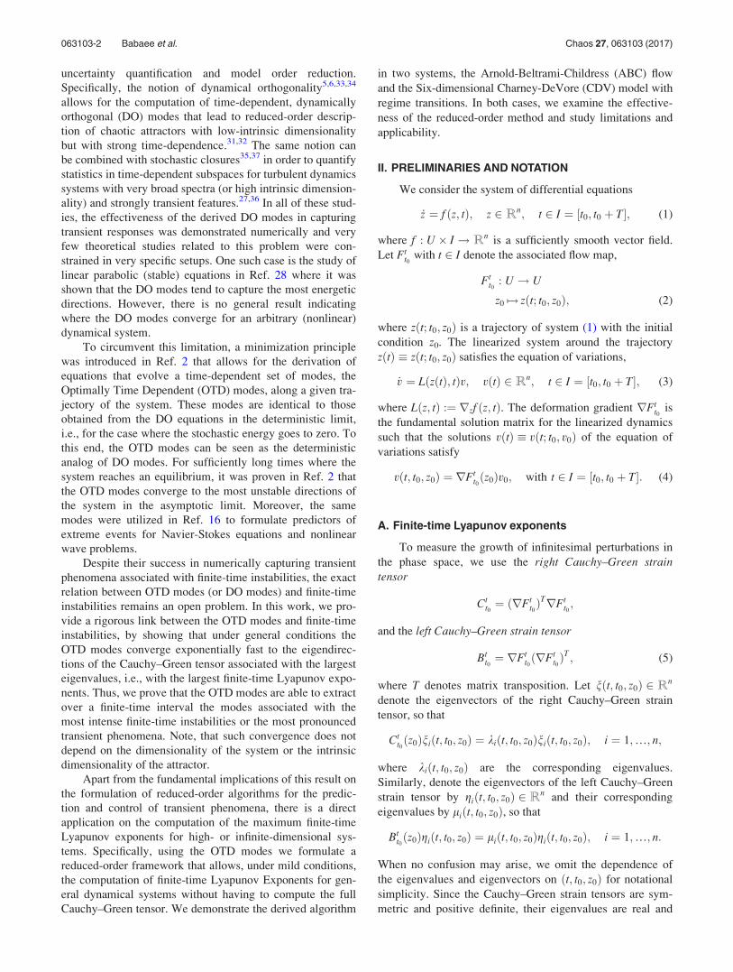
Figure 4 shows the reduced-order FTLE fields usingOTD reduction of sizes r¼ 1 (left column) and r¼ 2 (middlecolumn). The true FTLE field (right column) is also shownfor comparison. Each row of the figure shows a differentcross section of the field. For r¼ 2, the reduced-order FTLEis close to the true FTLE field. This is also true qualitativelyfor r¼ 1. However, for r¼ 1, the reduced FTLE exhibitsadditional troughs that do not exist in the true FTLE field.

We demonstrate in Fig. 5 that these false troughs occurwhen there is a crossing (or near crossing) between the first andsecond most dominant eigenvalues of the right Cauchy–Greentensor, i.e., k1 and k2. Recall that this eigenvalue crossing vio-lates condition (ii) of Theorem 3.2 and hence, the discrepancy

FIG. 3. The computational cost of the FTLE using the full system (28) (redcircles), and the reduced system (29) with r¼ 1 (black diamonds), r¼ 2(blue crosses), and r¼ 3 (green squares). The integer n is the system dimen-sion. The computational cost is measured as the number of scalar ODEs thatneed to be solved for each case.

063103-7 Babaee et al. Chaos 27, 063103 (2017)

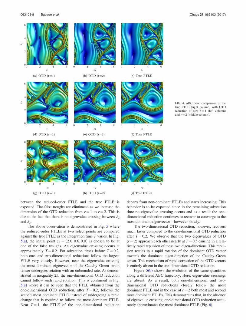
between the reduced-order FTLE and the true FTLE isexpected. The false troughs are eliminated as we increase thedimension of the OTD reduction from r¼ 1 to r¼ 2. This isdue to the fact that there is no eigenvalue crossing between k2

and k3.The above observation is demonstrated in Fig. 5 where

the reduced-order FTLEs at two select points are comparedagainst the true FTLE as the integration time T varies. In Fig.5(a), the initial point z0 ¼ ð2:0; 0:6; 0:0Þ is chosen to be atone of the false troughs. An eigenvalue crossing occurs atapproximately T¼ 0.2. For advection times before T¼ 0.2,both one- and two-dimensional reductions follow the largestFTLE very closely. However, near the eigenvalue crossingthe most dominant eigenvector of the Cauchy–Green straintensor undergoes rotation with an unbounded rate. As demon-strated in inequality 25, the one-dimensional OTD reductioncannot follow such rapid rotation. This is confirmed in Fig.5(a) where it can be seen that the FTLE obtained from theone-dimensional OTD reduction, after T¼ 0.2, follows thesecond most dominant FTLE instead of undergoing a rapidchange that is required to follow the most dominant FTLE.Near T¼ 1, the FTLE of the one-dimensional reduction

departs from non-dominant FTLEs and starts increasing. Thisbehavior is to be expected since in the remaining advectiontime no eignevalue crossing occurs and as a result the one-dimensional reduction continues to recover to converge to themost dominant eigenvector—however slowly.

The two-dimensional OTD reduction, however, recoversmuch faster compared to the one-dimensional OTD reductionafter T¼ 0.2. We observe that the two eigenvalues of OTD(r¼ 2) approach each other nearly at T¼ 0.5 causing in a rela-tively rapid repulsion of these two eigen-directions. This repul-sion results in a rapid rotation of the dominant OTD vectortowards the dominant eigen-direction of the Cauchy–Greentensor. This mechanism of rapid correction of the OTD vectorsis entirely absent in the one-dimensional OTD reduction.

Figure 5(b) shows the evolution of the same quantitiesalong a different ABC trajectory. Here, eigenvalue crossingsare absent. As a result, both one-dimensional and two-dimensional OTD reductions closely follow the mostdominant FTLE and in the case of r¼ 2 both most and secondmost dominant FTLEs. This demonstrates that, in the absenceof eigenvalue crossing, one-dimensional OTD reduction accu-rately approximates the most dominant FTLE (Fig. 6).

FIG. 4. ABC flow: comparison of thetrue FTLE (right column) with OTDreduction of size r¼ 1 (left column)and r¼ 2 (middle column).

063103-8 Babaee et al. Chaos 27, 063103 (2017)

FIG. 6. Six-dimensional Charney–DeVore model: comparison of the trueFTLE (rightmost column) with OTDreduction of size r¼ 1 (leftmost col-umn) and r¼ 2 middle column. Eachrow shows results of a section of thephase space.

FIG. 5. ABC flow: FTLE versus advection time calculated with full dynamics (solid blue), one-dimensional OTD reduction (dashed gray line with trianglesymbols) and two-dimensional OTD reduction (red line with circle symbols) with initial points of: (a) z0 ¼ ð2:0; 0:6; 0:0Þ, and (b) z0 ¼ ð4:0; 0:6; 0:0Þ. The ini-tial points are shown with a cross symbol in the z1 * z2 plane.

063103-9 Babaee et al. Chaos 27, 063103 (2017)

B. Charney–DeVore model with regime transitions

In this section, we apply the OTD reduction to the six-dimensional truncation of the equations for barotropic flowin a plane channel with orography that are known as theCharney–DeVore (CDV) model. The truncated system isgiven by

_z1 ¼ c/1z3 * Cðz1 * z/1Þ;_z2 ¼ *ða1z1 * b1Þz3 * Cz2 * d1z4z6;

_z3 ¼ ða1z1 * b1Þz2 * c1z1 * Cz3 þ d1z4z5;

_z4 ¼ c/2z6 * Cðc4 * z/4Þ þ !ðz2z6 * z3z5Þ;_z5 ¼ *ða2z1 * b2Þz6 * Cz5 * d2z4z3;

_z6 ¼ ða2z1 * b2Þz2 * c2z4 * Cz6 þ d2z4z2:

(31)

The model coefficients are given by

am ¼8ffiffiffi2p

pm2

4m2 * 1

b2 þ m2 * 1

b2 þ m2; bm ¼

bb2

b2 þ m2;

dm ¼64

ffiffiffi2p

15pb2 * m2 þ 1

b2 þ m2; c/m ¼ c

4m

4m2 * 1

ffiffiffi2p

b

p;

! ¼ 16ffiffiffi2p

5p; cm ¼ c

4m3

4m2 * 1

ffiffiffi2p

b

p b2 þ m2ð Þ :

(32)

Following Ref. 11, we set ðz/1; z/4;C; b; c; bÞ ¼ ð0:95;*0:76095; 0:1; 1:25; 0:2; 0:5Þ. For these parameters, theCDV model generates regime transitions due to the interac-tion of barotropic and topographic instabilities. It was shownin Ref. 10 that a Proper Orthogonal Decomposition (POD)reduction of this model to three leading POD modes resolves97% of cumulative variance but cannot capture the chaoticregime transitions present in the six-dimensional model.These highly transient instabilities render this model anappropriate test case for evaluating the performance of theOTD reduction in computing the FTLE. Moreover, usingthis model we assess the performance of the OTD reductionfor a higher dimensional problem.

We compute the true FTLE using the finite differencemethod analogous to the ABC flow problem. Similarly, theinitial condition U(0) for the OTD equation (29b) is the r mostdominant eigenvectors of the symmetric linearized operator.The fourth-order Runge-Kutta scheme with time step sizeDt ¼ 0:4 (days) is used for the numerical integration of Eqs.(28) and (29). Using the smaller time step Dt ¼ 0:2 (days) didnot change the numerical results.

Figure 6 shows the reduced FTLE fields obtained fromthe one-dimensional reduction (left column) and two-dimensional reduction (middle column) as well as the fullFTLE (right column). Each row shows a two-dimensionalcross section of the phase space. As in the ABC flow, thereduced FTLE fields agree qualitatively with the full FTLEfield. However, for r¼ 1 reduction, some false troughs areobserved. Away from the false troughs, the one-dimensionalreduction estimates the FTLE accurately. For r¼ 2 reduc-tion, there are no false troughs.

In Fig. 7, the FTLE values are plotted as a function ofthe integration time. These correspond to the pointz0 ¼ ð1:14; 0; 0;*0:91; 0; 0Þ, marked by a cross symbol in

the inset, which lies on a false trough in the z1 * z4 section.An eigenvalue crossing occurs at approximately T¼ 9.Analogous to the ABC flow, we observe that before T¼ 9both one- and two-dimensional OTD reductions capture themost dominant eigenvalues of the Cauchy–Green strain ten-sor. After T¼ 9, the one-dimensional OTD reduction contin-uously follows the second most dominant eigen-direction ofthe Cauchy–Green strain tensor. The inability of a singleOTD vector to undergo a dramatic rotation to follow themost dominant eigen-direction of the Cauchy–Green tensorleads to the false trough that is observed in Fig. 6(a). Thetwo-dimensional OTD subspace, however, converges to thesubspace spanned by the two most dominant eigenvectors ofthe Cauchy–Green strain tensor. This convergence is guaran-teed by Theorem 3.2 since the second and the thirdCauchy–Green eigenvalues ðk2; k3Þ do not cross (see Fig. 7).As a result, the two-dimensional (r¼ 2) OTD reductionclosely approximates the two large FTLEs for all times.

The above results demonstrate that, as long as k2 and k3

do not coincide, a reduced FTLE with two OTD modes reli-ably approximates the dominant FTLEs of the full systemregardless of the system’s dimension n. This amounts to asignificant reduction in the computational cost of the FTLEevaluations, and the gain in the computational speed is largeras the dimension of the dynamical system increases.Investigating the numerical performance of the OTD reduc-tion for infinite-dimensional systems is the subject of futurestudy.

VI. CONCLUSIONS

We have examined the properties of the optimally time-dependent (OTD) modes for general time-dependent dynam-ical systems. Specifically, we have shown that under mildconditions, related to the spectrum of the Cauchy–Green ten-sor, the OTD modes converge exponentially fast to the eigen-directions of the Cauchy–Green tensor associated with thedominant eigenvalues (largest finite-time Lyapunov expo-nents). Therefore, the OTD modes can be employed to

FIG. 7. Six-dimensional Charney–DeVore model: FTLE versus advectiontime calculated with full dynamics (solid blue), one-dimensional OTDreduction (dashed gray line with triangle symbols), and two-dimensionalOTD reduction (red line with circle symbols) with initial points of z0;1 ¼1:14; z0;4 ¼ *0:91 and other coordinates being zero. The initial point isshown with a cross symbol in the z1 * z4 plane.

063103-10 Babaee et al. Chaos 27, 063103 (2017)

extract time-dependent subspaces that encode informationassociated with the transient dynamics and accurately char-acterize the associated finite-time instabilities. This is animportant development relative to known shortcomings ofproper orthogonal decomposition models, which may changeor even invert stability characteristics.3,29

We have applied the derived result on the formulation ofa reduced order algorithm for the computation of the maxi-mum finite-time Lyapunov exponent, a measure that hasbeen used for the quantification of Lagrangian CoherentStructures. We demonstrated the derived results through twospecific examples, the three-dimensional ABC flow and thesix-dimensional Charney-DeVore model. In both cases, wethoroughly analyzed the limitations due to dimensionalityreduction in combination with eigenvalue crossing. Apartfrom its value as a computational method for finite-timeLyapunov exponents, the presented result paves the way forthe development of efficient control and prediction strategiesfor chaotic dynamical systems exhibiting transient features,such as extreme events and off-equilibrium dynamics.

ACKNOWLEDGMENTS

T.P.S. has been supported through the ARO Grant No.66710-EG-YIP, the AFOSR Grant No. FA9550-16-1-0231,the ONR Grant No. N00014-15-1-2381, and the DARPAGrant No. HR0011-14-1-0060. H.B. and M.F. have beensupported through the first, second, and fourth grants aspostdoctoral associates.

APPENDIX A: THE OTD MODES AND THEDYNAMICALLY ORTHOGONAL MODES

The set of OTD equations have the same form as theDynamically Orthogonal (DO) field equations.31,33 In fact,because the minimization of the function F is performed onlyover the rate of change of the basis elements, _uiðtÞ, [and not thebasis elements uiðtÞ] one can follow exactly the same steps asin Theorem 2.1 in Ref. 2 to show that the evolution equations(15) can be derived for the general case of a nonlinear operatorN ðUÞ. More specifically, by minimization of the functional

F _u1; _u2;…; _urð Þ ¼Xr

i¼1

""""@ui tð Þ@t*N z tð Þ;U tð Þ; tð Þ

""""2

; (A1)

we can obtain the evolution equations.

@U

@t¼ N Uð Þ * UUTN Uð Þ: (A2)

For the case of the DO equations, the nonlinear operatortakes the form

N ðUÞ ¼ Ex Lð!u þXr

i¼1

uiYiÞYj

" #C*1

YiYj; (A3)

where we have used the notation in Ref. 31, i.e., L is theright hand side of the stochastic partial differential equation(PDE), !u is the trajectory of the mean, YiðtÞ are the stochasticcoefficients and CYiYjðtÞ is their covariance matrix. The

operation Ex denotes the average with respect to an appro-priate probability measure. Conversely, one can obtain theOTD mode equations from the DO equations simply by con-sidering their deterministic limit, i.e., by taking the limitCYiYjðtÞ! 0.

APPENDIX B: PROOF OF THEOREM 4.1

We consider the rate of change of the eigenvectors of ageneral one-parameter family of symmetric matrices, GðtÞ2 Rn'n. For such a matrix, we have the eigenvalue problem

GðtÞRðtÞ ¼ RðtÞKðtÞ; (B1)

where the columns of RðtÞ 2 Rn'n are the eigenvectorsof G(t) and KðtÞ 2 Rn'n is the diagonal matrix of corre-sponding eigenvalues. Note that, since G is symmetric, itseigenvectors are orthogonal and therefore, RRT ¼ I.Differentiating with respect to time, we obtain

_GRþ G _R ¼ _RKþ R _K:

Multiplying the above equation by RT from the left yields

_K ¼ RT _GRþ K RT _R * RT _RK:

Since RTR ¼ I, we have:

_RTRþ RT _R ¼ 0:

Let K ¼ RT _R. From the above relation, we observe that K isa skew-symmetric matrix. Denoting ~G ¼ RT _GR, we have

_K ¼ ~G þ KK * KK:

For off-diagonal terms i 6¼ j, we have _Kij ¼ 0. Therefore,

~Gij ¼ kjKij * kiKij; i 6¼ j:

Transposing the above relation

~Gji ¼ kiKji * kjKji; i 6¼ j:

Using the skew-symmetric property of K, i.e., Kij ¼ *Kji,and summing up the above two equations yields

Kij ¼~Gij þ ~Gji

2 kj * ki# $ ; i 6¼ j: (B2)

This results in the following closed-form evolution equationsfor K and R,

_K ¼ diagð ~GÞ; (B3)

_R ¼ RK: (B4)

1V. I. Arnold and B. A. Khesin, Topological Methods in Hydrodynamics(Springer, 1998), Vol. 125.

2H. Babaee and T. P. Sapsis, “A minimization principle for the descriptionof modes associated with finite-time instabilities,” Proc. R. Soc. A 472,20150779 (2016).

3S. L. Brunton and B. R. Noack, “Closed-loop turbulence control: Progressand challenges,” Appl. Mech. Rev. 67, 050801 (2015).

063103-11 Babaee et al. Chaos 27, 063103 (2017)

4G. J. Chandler and R. R. Kerswell, “Invariant recurrent solutions embed-ded in a turbulent two-dimensional Kolmogorov flow,” J. Fluid Mech.722, 554–595 (2013).

5M. Cheng, T. Hou, and Z. Zhang, “A dynamically bi-orthogonal methodfor time-dependent stochastic PDEs I: Adaptivity and generalizations,”J. Comput. Phys. 242, 753–776 (2013).

6M. Cheng, T. Hou, and Z. Zhang, “A dynamically bi-orthogonal methodfor time-dependent stochastic PDEs I: Derivation and algorithms,”J. Comput. Phys. 242, 843–868 (2013).

7S. P. Cornelius, W. L. Kath, and A. E. Motter, “Realistic control of net-work dynamics,” Nat. Commun. 4, 1942 (2013).

8W. Cousins and T. P. Sapsis, “Quantification and prediction of extremeevents in a one-dimensional nonlinear dispersive wave model,” Physica D280, 48–58 (2014).

9W. Cousins and T. P. Sapsis, “Reduced order precursors of rare events inunidirectional nonlinear water waves,” J. Fluid Mech. 790, 368–388(2016).

10D. T. Crommelin and A. J. Majda, “Strategies for model reduction:Comparing different optimal bases,” J. Atmos. Sci. 61(17), 2206–2217(2004).

11D. T. Crommelin, J. D. Opsteegh, and F. Verhulst, “A mechanism foratmospheric regime behavior,” J. Atmos. Sci. 61(12), 1406–1419(2004).

12M. Farazmand, D. Blazevski, and G. Haller, “Shearless transport barriersin unsteady two-dimensional flows and maps,” Physica D 278–279, 44–57(2014).

13M. Farazmand and G. Haller, “Computing Lagrangian coherent structuresfrom their variational theory,” Chaos 22, 013128 (2012).

14M. Farazmand and G. Haller, “Attracting and repelling Lagrangian coher-ent structures from a single computation,” Chaos 4, 023101 (2013).

15M. Farazmand and G. Haller, “Polar rotation angle identifies ellipticislands in unsteady dynamical systems,” Physica D 315, 1–12 (2016).

16M. Farazmand and T. P. Sapsis, “Dynamical indicators for the predictionof bursting phenomena in high-dimensional systems,” Phys. Rev. E 94,032212 (2016).

17M. Farazmand and T. P. Sapsis, “Reduced-order prediction of rogue wavesin two-dimensional deep-water waves,” J. Comput. Phys. 340, 418–434(2017).

18F. Ginelli, P. Poggi, A. Turchi, H. Chat"e, R. Livi, and A. Politi,“Characterizing dynamics with covariant Lyapunov vectors,” Phys. Rev.Lett. 99(13), 130601 (2007).

19G. Haller, “Distinguished material surfaces and coherent structures in 3Dfluid flows,” Physica D 149, 248–277 (2001).

20G. Haller, “Lagrangian structures and the rate of strain in a partition oftwo-dimensional turbulence,” Phys. Fluids 13(11), 3365–3385 (2001).

21G. Haller and T. Sapsis, “Localized instability and attraction along invari-ant manifolds,” SIAM J. Appl. Dyn. Syst. 9(2), 611–633 (2010).

22G. Haller and G. Yuan, “Lagrangian coherent structures and mixing intwo-dimensional turbulence,” Physica D 147, 352–370 (2000).

23D. Karrasch, M. Farazmand, and G. Haller, “Attraction-based computationof hyperbolic Lagrangian coherent structures,” J. Comput. Dyn. 2(1),83–93 (2015).

24P. Lancaster, “On eigenvalues of matrices dependent on a parameter,”Numer. Math. 6, 377 (1964).

25F. Lekien and S. D. Ross, “The computation of finite-time Lyapunov expo-nents on unstructured meshes and for non-Euclidean manifolds,” Chaos20, 017505 (2010).

26F. Lekien, S. Shadden, and J. Marsden, “Lagrangian coherent structures inn-dimensional systems,” J. Math. Phys. 48, 065404 (2007).

27A. J. Majda, D. Qi, and T. P. Sapsis, “Blended particle filters for large-dimensional chaotic dynamical systems,” Proc. Natl. Acad. Sci. 111(21),7511–7516 (2014).

28E. Musharbash, F. Nobile, and T. Zhou, “Error analysis of the dynamicallyorthogonal approximation of time dependent random PDEs,” SIAM J. Sci.Comput. 37(2), A776–A810 (2015).

29B. R. Noack, K. Afanasiev, M. Morzynski, G. Tadmor, and F. Thiele, “Ahierarchy of low-dimensional models for the transient and post-transientcylinder wake,” J. Fluid Mech. 497, 335 (2003).

30W. Ott and J. A. Yorke, “When lyapunov exponents fail to exist,” Phys.Rev. E 78(5), 056203 (2008).

31T. P. Sapsis, “Attractor local dimensionality, nonlinear energy transfers,and finite-time instabilities in unstable dynamical systems with applica-tions to 2D fluid flows,” Proc. R. Soc. A 469(2153), 20120550 (2013).

32T. P. Sapsis and H. A. Dijkstra, “Interaction of noise and nonlinear dynam-ics in the double-gyre wind-driven ocean circulation,” J. Phys. Oceanogr.43, 366–381 (2013).

33T. P. Sapsis and P. F. J. Lermusiaux, “Dynamically orthogonal field equa-tions for continuous stochastic dynamical systems,” Physica D 238,2347–2360 (2009).

34T. P. Sapsis and P. F. J. Lermusiaux, “Dynamical criteria for the evolutionof the stochastic dimensionality in flows with uncertainty,” Physica D 241,60 (2012).

35T. P. Sapsis and A. J. Majda, “A statistically accurate modified quasilinearGaussian closure for uncertainty quantification in turbulent dynamical sys-tems,” Physica D 252, 34–45 (2013).

36T. P. Sapsis and A. J. Majda, “Blending modified Gaussian closure andnon-gaussian reduced subspace methods for turbulent dynamical systems,”J. Nonlinear Sci. 23, 1039 (2013).

37T. P. Sapsis and A. J. Majda, “Statistically accurate low order models foruncertainty quantification in turbulent,” Proc. Natl. Acad. Sci. 110,13705–13710 (2013).

38Y. Susuki, I. Mezic, and I. Mezic, “Nonlinear Koopman modes and a pre-cursor to power system swing instabilities,” IEEE Trans. Power Syst.27(3), 1182–1191 (2012).

063103-12 Babaee et al. Chaos 27, 063103 (2017)