sliding mode: basic theory and new perspectivesdelbuono/usai_talk_1.pdf · • regularization of...
TRANSCRIPT
SDS 2008 - Capitolo (BA) June 2008 1/54
Dept of Electrical and Electronic Eng.Dept of Electrical and Electronic Eng.University ofUniversity of CagliariCagliari
5th Workshop on
Structural Dynamical Systems: Computational Aspects
Capitolo (BA) – Italy
Sliding mode:
Basic theory and new perspectives
Elio USAI
SDS 2008 - Capitolo (BA) June 2008 2/54
Summary
• Switching systems
• Introductive examples
• Zeno behaviour
• Sliding modes in switching systems
• Regularization of sliding a mode trajectory
• Sliding modes in control systems
• Stability of a sliding mode control system
• Invariance of a sliding mode control system
• Recovering the uncertain dynamics
• Approximability
• Discrete time implementation
• Higher order sliding modes
SDS 2008 - Capitolo (BA) June 2008 3/54
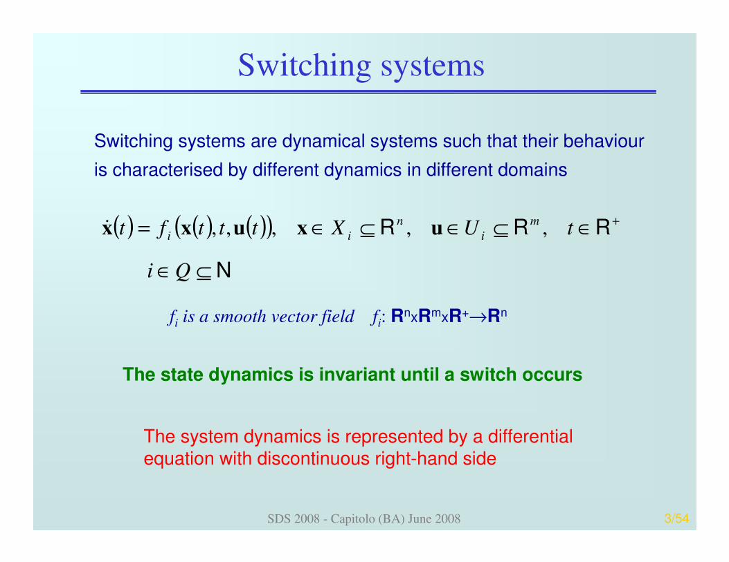
Switching systems
Switching systems are dynamical systems such that their behaviour
is characterised by different dynamics in different domains
( ) ( ) ( )( )
N
RRR
⊆∈
∈⊆∈⊆∈= +
Qi
tUXtttftm
i
n
ii ,,,,, uxuxx&
fi is a smooth vector field fi: RnxRmxR+→Rn
The state dynamics is invariant until a switch occurs
The system dynamics is represented by a differential equation with discontinuous right-hand side
SDS 2008 - Capitolo (BA) June 2008 4/54
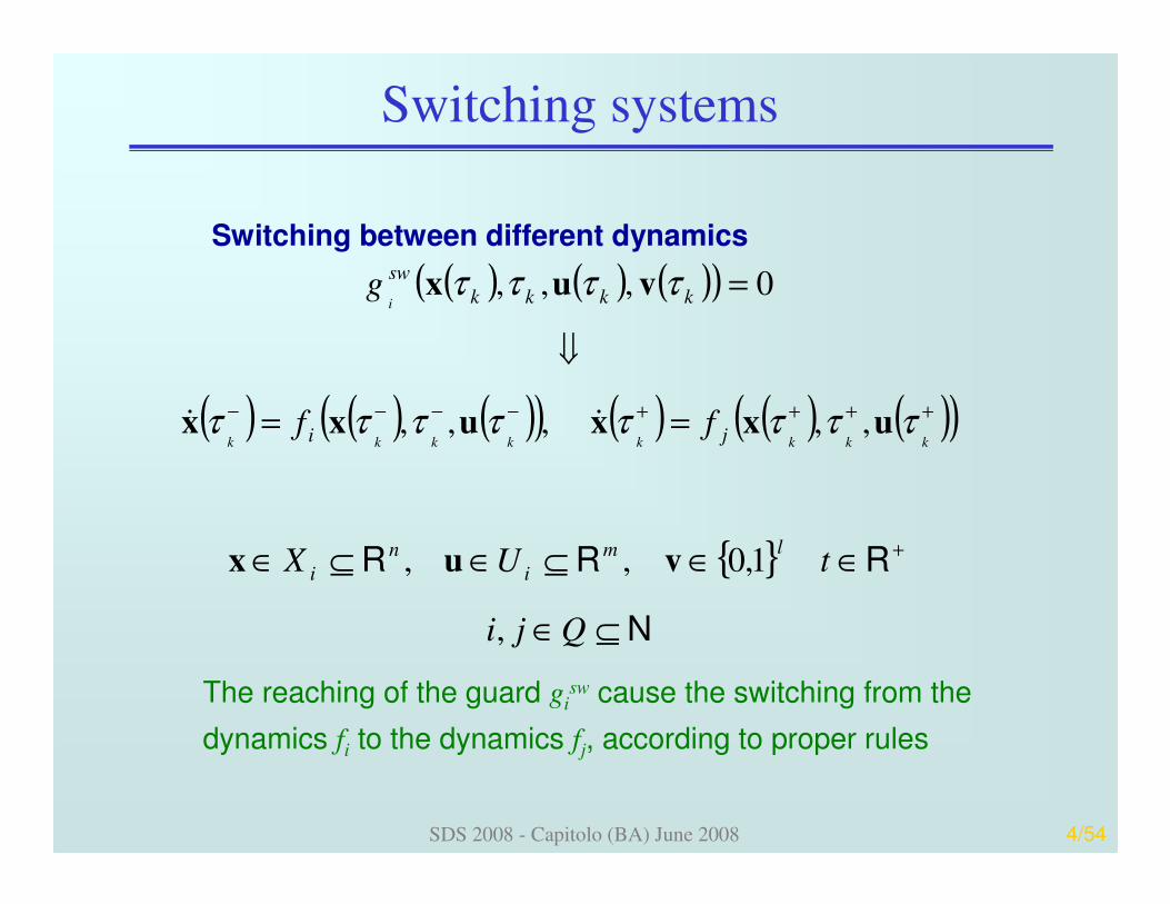
Switching systems
Switching between different dynamics
( ) ( ) ( )( )
( ) ( ) ( )( ) ( ) ( ) ( )( )
N
RRR
⊆∈
∈∈⊆∈⊆∈
==
⇓
=
+
++++−−−−
Qji
tUX
ff
g
lm
i
n
i
ji
kkkk
sw
kkkkkkkk
i
,
1,0,,
,, ,,,
0,,,
vux
uxxuxx
vux
ττττττττ
ττττ
&&
The reaching of the guard gisw cause the switching from the
dynamics fi to the dynamics fj, according to proper rules
SDS 2008 - Capitolo (BA) June 2008 5/54
Switching systems
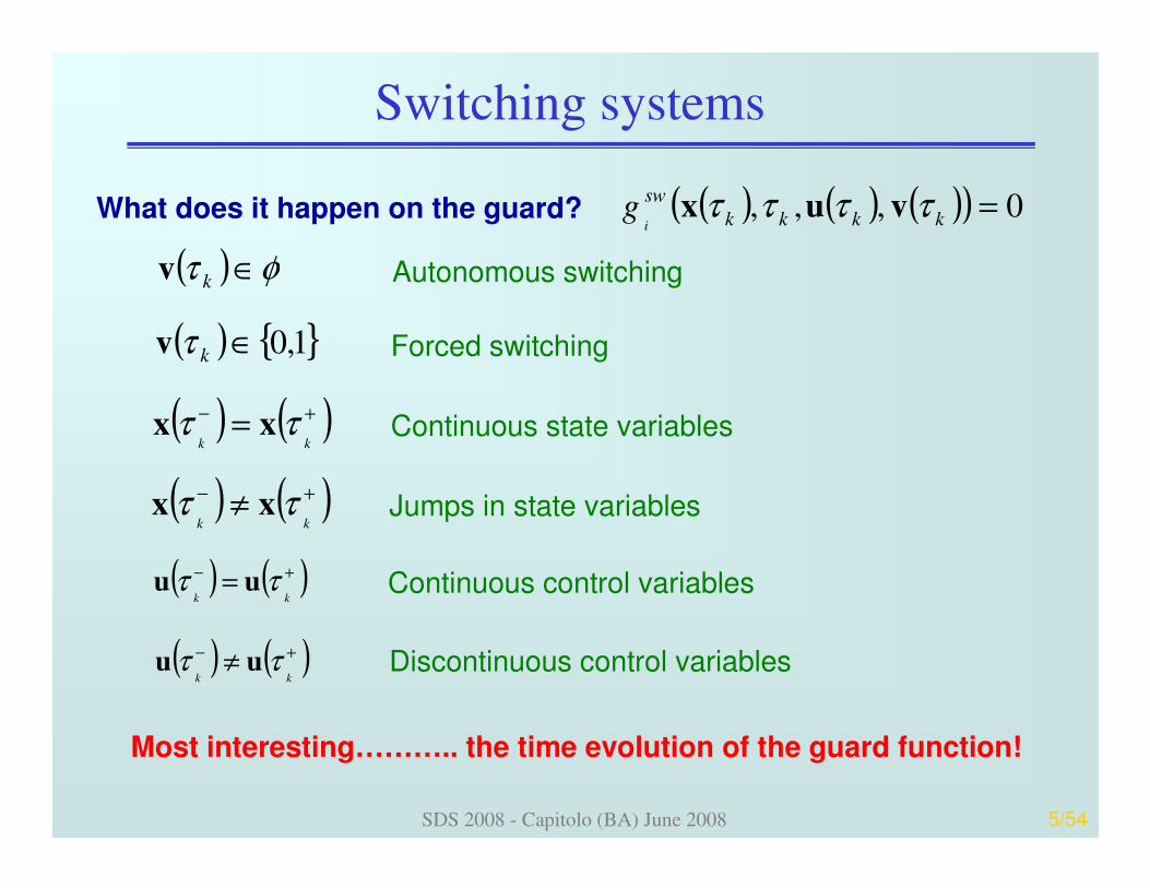
What does it happen on the guard? ( ) ( ) ( )( ) 0,,, =kkkk
sw
ig ττττ vux
( ) 1,0∈kτv Forced switching
( ) ( )+− =kk
ττ xx Continuous state variables
( ) ( )+− =kk
ττ uu Continuous control variables
( ) ( )+− ≠kk
ττ xx Jumps in state variables
( ) ( )+− ≠kk
ττ uu Discontinuous control variables
Most interesting……….. the time evolution of the guard function!
( ) φτ ∈kv Autonomous switching
SDS 2008 - Capitolo (BA) June 2008 6/54
Introductive examples
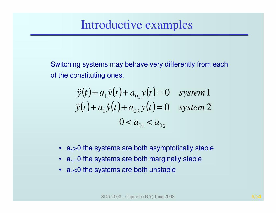
Switching systems may behave very differently from each
of the constituting ones.
( ) ( ) ( )( ) ( ) ( )
2010
201
101
0
20
10
aa
systemtyatyaty
systemtyatyaty
<<
=++
=++
&&&
&&&
• a1>0 the systems are both asymptotically stable
• a1=0 the systems are both marginally stable
• a1<0 the systems are both unstable
SDS 2008 - Capitolo (BA) June 2008 7/54
Introductive examples
-3 -2 -1 0 1 2 3
-3
-2
-1
0
1
2
3
y(t)
dy(t
)/dt
Phase plane
a0
1
=0.5
a0
2
=9.0
-10 -5 0 5 10-5
0
5
10
15
20Phase plane
y(t)
dy(t
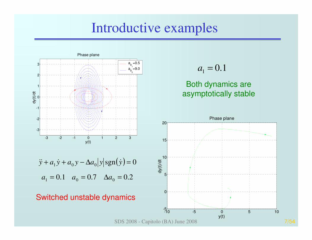
)/dt( )
2.07.01.0
0sgn
001
001
=∆==
=∆−++
aaa
yyayayay &&&&
1.01 =a
Switched unstable dynamics
Both dynamics are asymptotically stable
SDS 2008 - Capitolo (BA) June 2008 8/54
Introductive examples
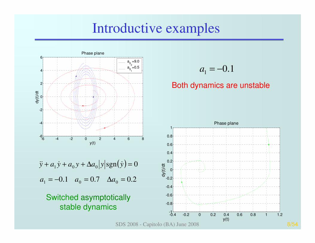
1.01 −=a
Switched asymptoticallystable dynamics
Both dynamics are unstable
-0.4 -0.2 0 0.2 0.4 0.6 0.8 1 1.2-1
-0.8
-0.6
-0.4
-0.2
0
0.2
0.4
0.6
0.8
1Phase plane
y(t)
dy(t
)/dt
-6 -4 -2 0 2 4 6 8-6
-4
-2
0
2
4
6
y(t)
dy(t
)/dt
Phase plane
a0
2
=9.0
a0
1
=0.5
( )
2.07.01.0
0sgn
001
001
=∆=−=
=∆+++
aaa
yyayayay &&&&
SDS 2008 - Capitolo (BA) June 2008 9/54
Introductive examples
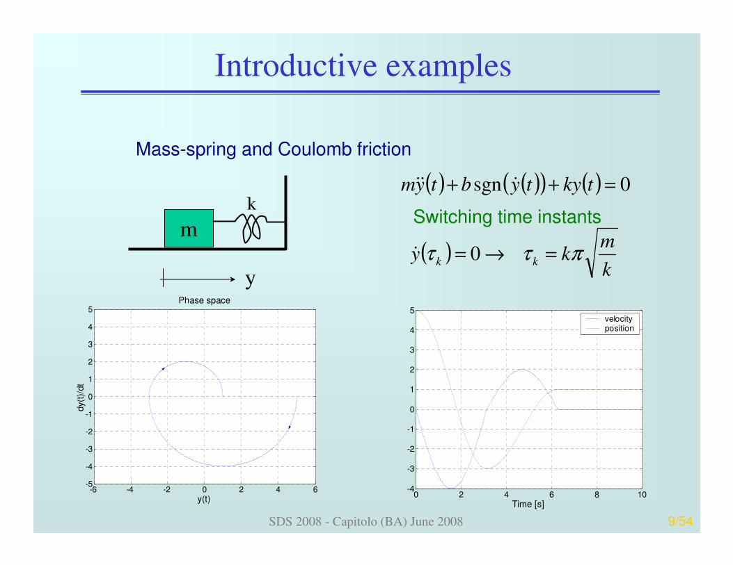
Mass-spring and Coulomb friction
( ) ( )( ) ( ) 0sgn =++ tkytybtym &&&
Switching time instantsm
k
y( )
k
mky kk πττ =→= 0&
-6 -4 -2 0 2 4 6-5
-4
-3
-2
-1
0
1
2
3
4
5Phase space
y(t)
dy(t
)/dt
0 2 4 6 8 10-4
-3
-2
-1
0
1
2
3
4
5
Time [s]
velocityposition
SDS 2008 - Capitolo (BA) June 2008 10/54
Introductive examples
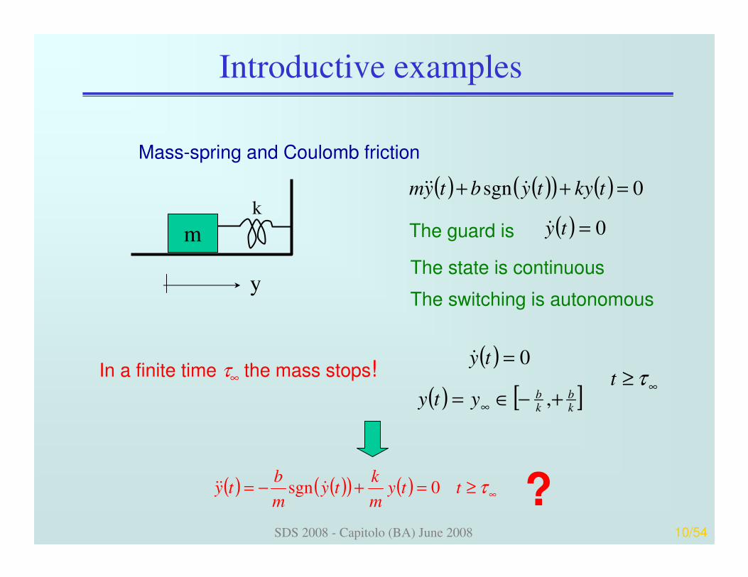
Mass-spring and Coulomb friction
( ) ( )( ) ( ) 0sgn =++ tkytybtym &&&
The guard is m
k
y
( ) 0=ty&
In a finite time τ∞ the mass stops!( )
( ) [ ]∞
∞
≥+−∈=
=τt
yty
ty
kb
kb
,
0&
The state is continuous
The switching is autonomous
( ) ( )( ) ( ) ∞≥=+−= τttym
kty
m
bty 0sgn &&& ?
SDS 2008 - Capitolo (BA) June 2008 11/54
Introductive examples
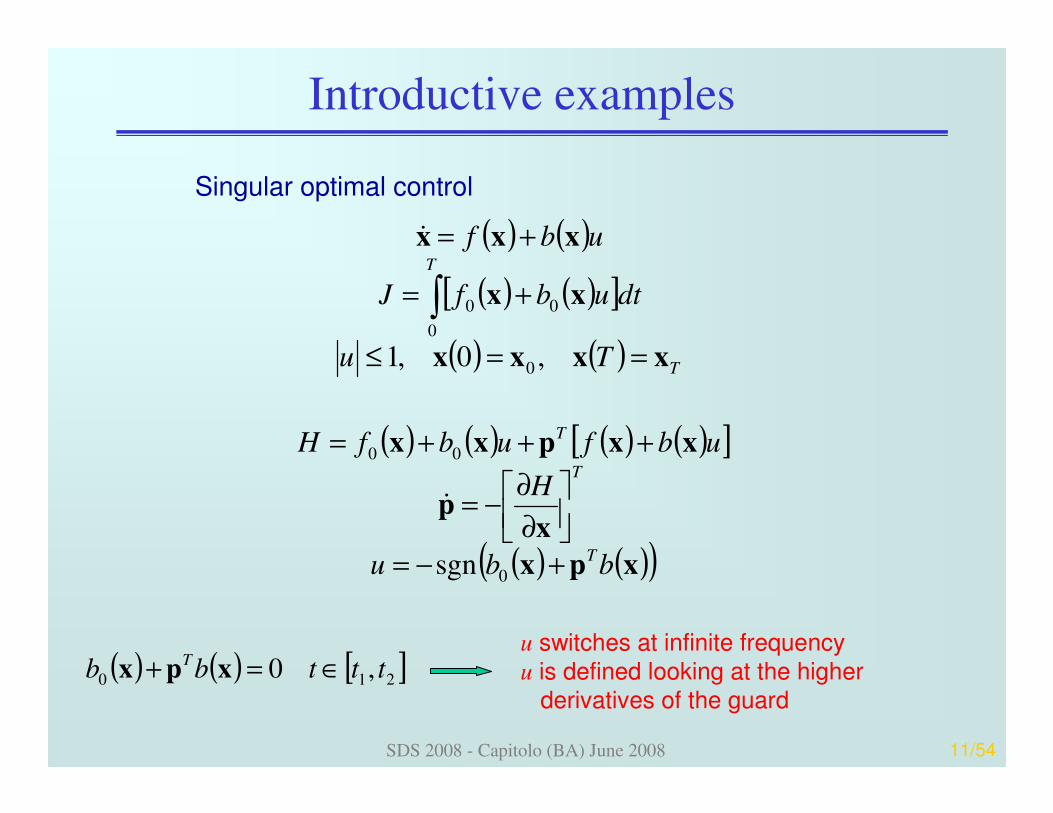
Singular optimal control
( ) ( )
( ) ( )[ ]
( ) ( ) T
T
Tu
dtubfJ
ubf
xxxx
xx
xxx
==≤
+=
+=
∫,0,1 0
0
00
&
( ) ( ) ( ) ( )[ ]
( ) ( )( )xpx
xp
xxpxx
bbu
H
ubfubfH
T
T
T
+−=
∂
∂−=
+++=
0
00
sgn
&
( ) ( ) [ ]210 ,0 tttbb T ∈=+ xpxu switches at infinite frequency
u is defined looking at the higher
derivatives of the guard
SDS 2008 - Capitolo (BA) June 2008 12/54
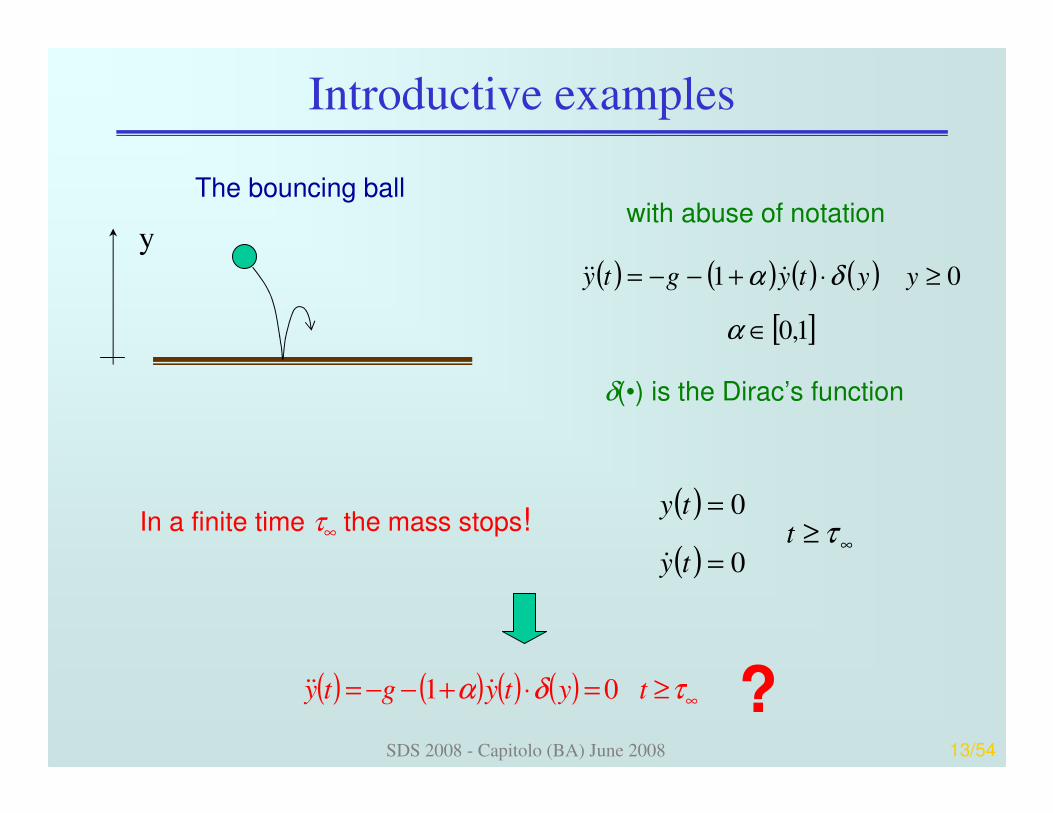
Introductive examples
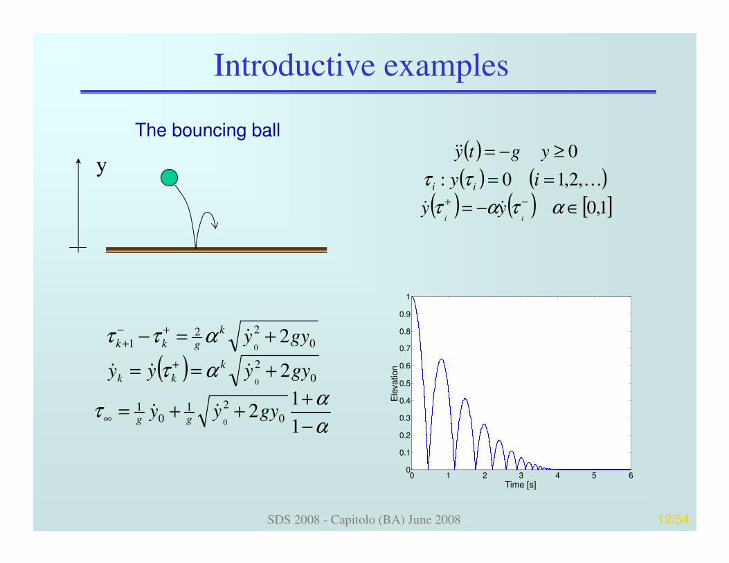
The bouncing ball( )( ) ( )
( ) ( ) [ ]1,0
,2,10:
0
∈−=
==
≥−=
−+ ατατ
ττ
iiyy
iy
ygty
ii
&&
K
&&y
0 1 2 3 4 5 60
0.1
0.2
0.3
0.4
0.5
0.6
0.7
0.8
0.9
1
Time [s]
Ele
vation( )
α
ατ
ατ
αττ
−
+++=
+==
+=−
∞
+
+−+
1
12
2
2
0
210
1
0
2
0
221
0
0
0
gyyy
gyyyy
gyy
gg
k
kk
k
gkk
&&
&&&
&
SDS 2008 - Capitolo (BA) June 2008 13/54
Introductive examples
The bouncing ball
( ) ( ) ( ) ( )
[ ]1,0
01
∈
≥⋅+−−=
α
δα yytygty &&&
ywith abuse of notation
δ(•) is the Dirac’s function
In a finite time τ∞ the mass stops!( )
( )∞≥
=
=τt
ty
ty
0
0
&
( ) ( ) ( ) ( ) ∞≥=⋅+−−= τδα tytygty 01 &&& ?
SDS 2008 - Capitolo (BA) June 2008 14/54
Zeno behaviour
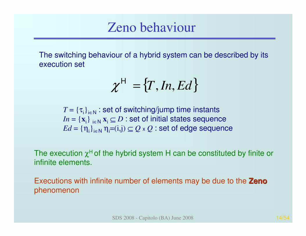
T = τii∈N : set of switching/jump time instantsIn = xi i∈N xi ⊆ D : set of initial states sequenceEd = ηii∈N ηi=(i,j) ⊆ Q x Q : set of edge sequence
EdInT ,,=Hχ
The execution χH of the hybrid system H can be constituted by finite or infinite elements.
Executions with infinite number of elements may be due to the ZenoZenophenomenon
The switching behaviour of a hybrid system can be described by its execution set

SDS 2008 - Capitolo (BA) June 2008 15/54
Zeno behaviour
The Zeno phenomenon appears when the execution χH of the
hybrid system is such that
( ) ∞<=−= ∞
∞
=+
∞→∑ ττττ
0
1limi
iiii
τ∞ (Zeno time) is a right accumulation point for the time instants sequence
( ) 01∞→
+ →−i
ii ττ The switching frequency tends to be infinite
In a Zeno condition the system evolves along a guard
( )( ) ( ) ∞≥∀=⋅∂
∂τtt
ttg0
,x
x
x&

SDS 2008 - Capitolo (BA) June 2008 16/54
Sliding modes in switching systems
The Zeno phenomenon is mainly related to the switching frequencyon a guard, but previous relationship shows the relation between the guard and the system dynamics
( )( ) 0, =ttg x( ) ( )( )ttft ,1 xx =&
( ) ( )( )ttft ,2 xx =&
( ) ( )( )ttft s ,xx =&
( )( )x
x
∂
∂ ttg ,
The motion of the system on a discontinuity surface is called sliding mode
SDS 2008 - Capitolo (BA) June 2008 17/54
Sliding modes in switching systems
Sliding modes are Zeno behaviours in switching
systems
The system is constrained onto a surface in the
state space, the sliding surface
When the system is constrained on the sliding
surface, the system modes differ from those of the original systems
The system is invariant when constrained on the sliding surface
Any system on the sliding surface behaves the same way
SDS 2008 - Capitolo (BA) June 2008 18/54
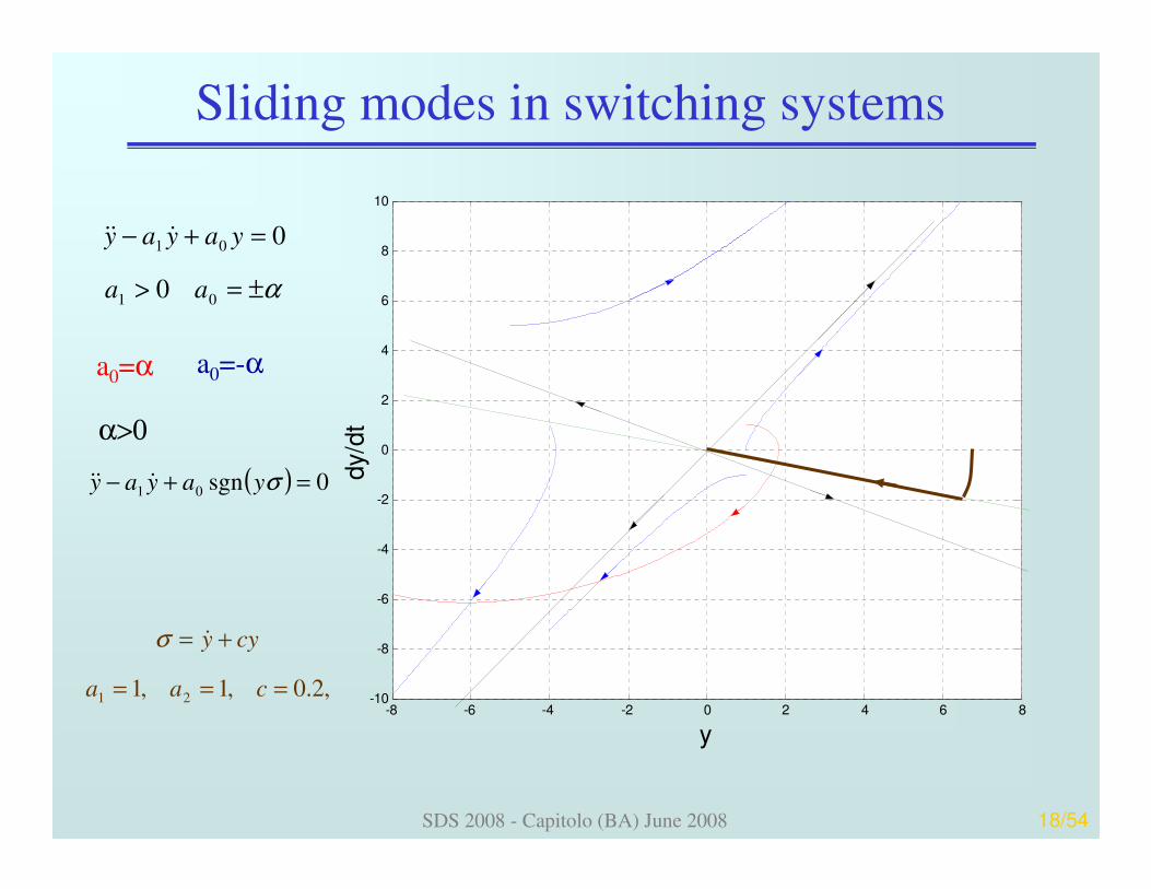
Sliding modes in switching systems
α±=>
=+−
01
01
0
0
aa
yayay &&&
a0=α a0=-α
α>0
( ) 0sgn01 =+− σyayay &&&
,2.0,1,1 21 ===
+=
caa
cyy&σ
-8 -6 -4 -2 0 2 4 6 8-10
-8
-6
-4
-2
0
2
4
6
8
10
y
dy/d
t
SDS 2008 - Capitolo (BA) June 2008 19/54
Sliding modes in switching systems
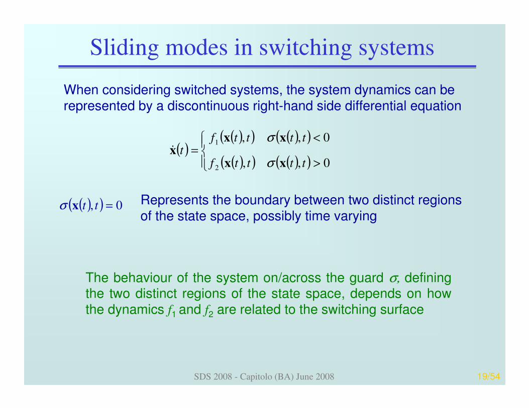
When considering switched systems, the system dynamics can be represented by a discontinuous right-hand side differential equation
( )( ) 0, =ttxσ
( )( )( ) ( )( )
( )( ) ( )( )
>
<=
0,,
0,,
2
1
ttttf
ttttft
xx
xxx
σ
σ&
Represents the boundary between two distinct regions of the state space, possibly time varying
The behaviour of the system on/across the guard σ, defining the two distinct regions of the state space, depends on how the dynamics f1 and f2 are related to the switching surface

SDS 2008 - Capitolo (BA) June 2008 20/54
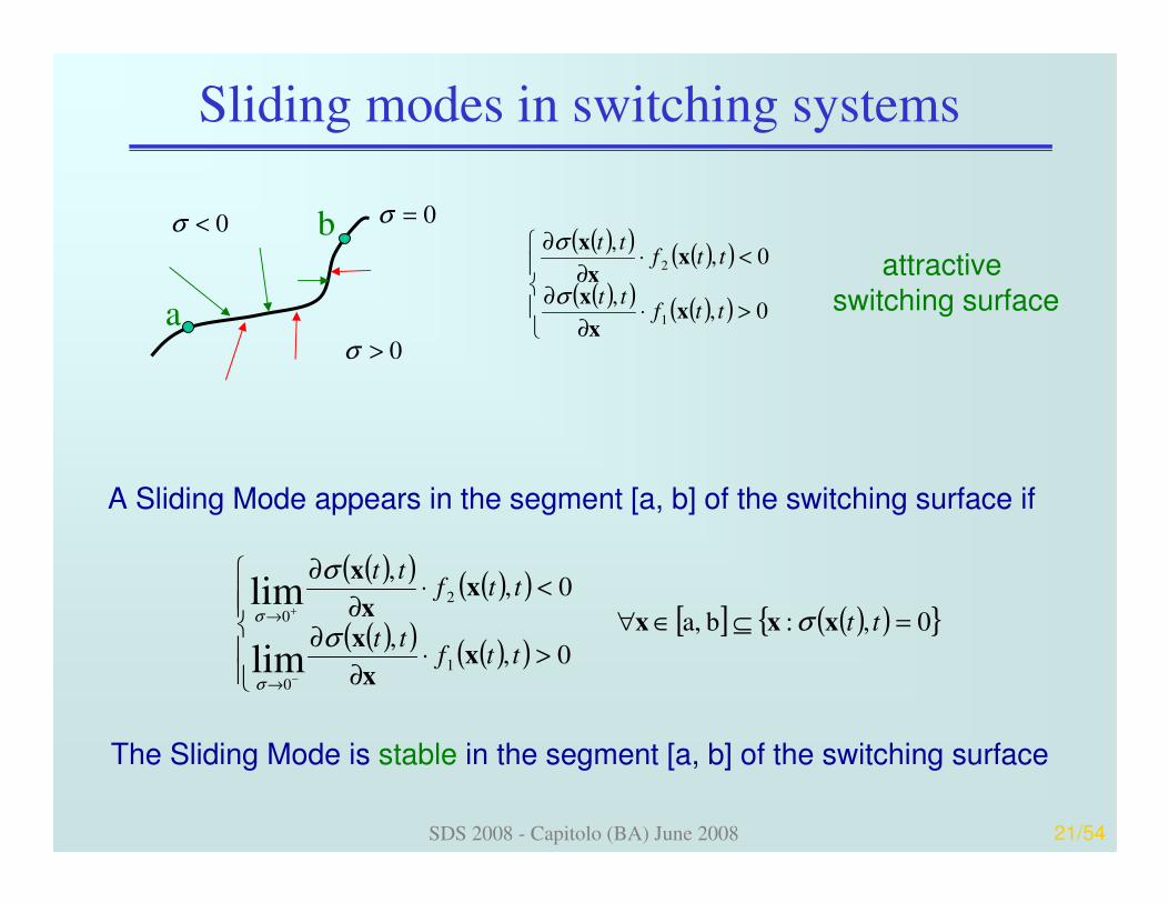
Sliding modes in switching systems
0>σ
0<σ 0=σ( )( ) ( )( )
( )( ) ( )( )
>⋅∂
∂
<⋅∂
∂
0,,
0,,
1
2
ttftt
ttftt
xx
x
xx
x
σ
σattractive
switching surface
0>σ
0<σ 0=σ( )( ) ( )( )
( )( ) ( )( )
<⋅∂
∂
>⋅∂
∂
0,,
0,,
1
2
ttftt
ttftt
xx
x
xx
x
σ
σrepulsive
switching surface
0>σ
0<σ 0=σ( )( ) ( )( )
( )( ) ( )( )
>⋅∂
∂
<⋅∂
∂
0,,
0,,
1
2
ttftt
ttftt
xx
x
xx
x
σ
σacross
switching surface
SDS 2008 - Capitolo (BA) June 2008 21/54
Sliding modes in switching systems
0>σ
0<σ 0=σ( )( ) ( )( )
( )( ) ( )( )
>⋅∂
∂
<⋅∂
∂
0,,
0,,
1
2
ttftt
ttftt
xx
x
xx
x
σ
σattractive
switching surface
A Sliding Mode appears in the segment [a, b] of the switching surface if
a
b
( )( ) ( )( )
( )( ) ( )( )[ ] ( )( ) 0,:b a,
0,,
0,,
1
0
2
0
lim
lim=⊆∈∀
>⋅∂
∂
<⋅∂
∂
−
+
→
→ tt
ttftt
ttftt
xxx
xx
x
xx
x
σσ
σ
σ
σ
The Sliding Mode is stable in the segment [a, b] of the switching surface

SDS 2008 - Capitolo (BA) June 2008 22/54
Regularization of a sliding mode trajectory
Considering the switched dynamics
( )
( )( ) ( )( )
( )( ) ( )( )
( )( ) ( )( )
>
=
<
=
0,,
0,,
0,,
2
1
ttttf
ttttf
ttttf
t s
xx
xx
xx
x
σ
σ
σ
&
Regularization of the sliding mode implies to find the continuous vector
function fs such that the state trajectory remains on the switching surface
Filippov’s continuation method
Equivalent dynamics method (“equivalent control”)
SDS 2008 - Capitolo (BA) June 2008 23/54
Regularization of a sliding mode trajectory
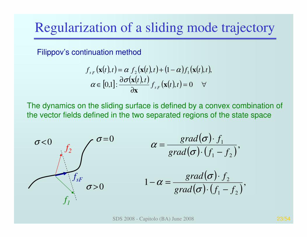
Filippov’s continuation method
( )( ) ( )( ) ( ) ( )( )
[ ] ( )( ) ( )( ) ∀=∂
∂∈
−+=
0,,
:1,0
,,1, , 12
ttftt
ttfttfttf
Fs
Fs
xx
x
xxx
σα
αα
The dynamics on the sliding surface is defined by a convex combination of the vector fields defined in the two separated regions of the state space
0>σ
0<σ 0=σ
f1
f2
fsF
( )( ) ( )
( )( ) ( )
,1
,
21
2
21
1
ffgrad
fgrad
ffgrad
fgrad
−⋅
⋅=−
−⋅
⋅=
σ
σα
σ
σα
SDS 2008 - Capitolo (BA) June 2008 24/54
Regularization of a sliding mode trajectory
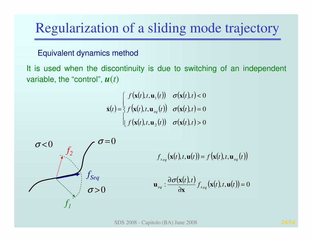
Equivalent dynamics method
( ) ( )( ) ( ) ( )( )
( )( ) ( ) ( )( ) 0,,,
:
,, ,,
=∂
∂
=
tttftt
tttftttf
eqseq
eqeqs
uxx
xu
uxux
σ
It is used when the discontinuity is due to switching of an independent
variable, the “control”, u(t)
0>σ
0<σ 0=σ
f1
f2
fSeq
( )
( ) ( )( ) ( )( )
( ) ( )( ) ( )( )
( ) ( )( ) ( )( )
>
=
<
=
0,,,
0,,,
0,,,
2
1
tttttf
tttttf
tttttf
t eq
xux
xux
xux
x
σ
σ
σ
&

SDS 2008 - Capitolo (BA) June 2008 25/54
Regularization of a sliding mode trajectory
Filippov’s continuation method and the equivalent control method can give different solutions in nonlinear systemsFilippov’s continuation method and the equivalent control method can give different solutions in nonlinear systems
Not uniqueness problems in finding the solution of the sliding mode dynamics
In real systems such motions appear in representing constrained systems, or in control systems in which a variable is forced to be zero
Presence of more than a single switching surface
In most cases the uniqueness problem does not arise
SDS 2008 - Capitolo (BA) June 2008 26/54
Sliding modes in control systems
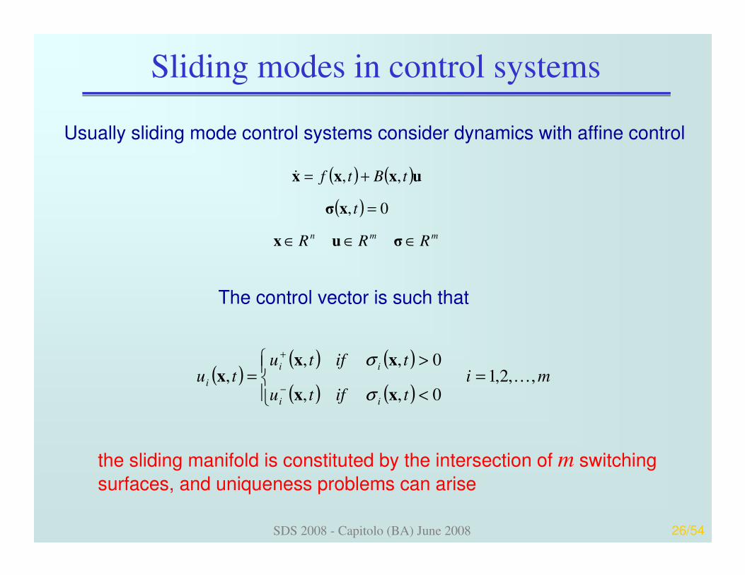
Usually sliding mode control systems consider dynamics with affine control
( ) ( )
( )mmn
RRR
t
tBtf
∈∈∈
=
+=
σux
xσ
uxxx
0,
,,&
The control vector is such that
( )( ) ( )
( ) ( )mi
tiftu
tiftutu
ii
ii
i ,,2,1 0,,
0,,, K=
<
>=
−
+
xx
xxx
σ
σ
the sliding manifold is constituted by the intersection of m switching
surfaces, and uniqueness problems can arise

SDS 2008 - Capitolo (BA) June 2008 27/54
Stability of a sliding mode control system
Local stability of a sliding mode on the domain
S(t)=σσσσ: σi=0; i=1,2,…,m
can be stated by the following Lyapunov-like theorem
The subspace S(t) is a sliding domain if a function V(σσσσ,x, t) exists in a
domain Ω of the space σ1, σ2, …, σm containing the origin such that:
• V(σσσσ,x, t) is positive definite with respect to σ,σ,σ,σ, for all x and any t
• On the sphere ||σσσσ||=R, for all x and any t, the function V(σσσσ,x, t) remains bounded
• The total time derivative of function V(σσσσ,x, t)
is negative everywhere except on the discontinuity surfaces where it is not defined
• On the sphere ||σσσσ||=R, for all x and any t, the total time derivative of
V(σσσσ,x, t) is upper bounded by a negative constant
( )t
VBf
VVV
∂
∂++
∂
∂+
∂
∂
∂
∂= u
xx
σ
σ
&
SDS 2008 - Capitolo (BA) June 2008 28/54
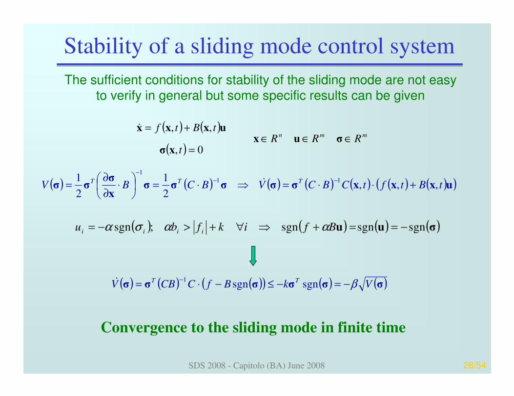
Stability of a sliding mode control system
The sufficient conditions for stability of the sliding mode are not easy to verify in general but some specific results can be given
( ) ( )
( )mmn
RRRt
tBtf∈∈∈
=
+=σux
xσ
uxxx
0,
,,&
( ) ( ) ( ) ( ) ( ) ( ) ( )( )uxxxσσσσσx
σσσ tBtftCBCVBCBV
TTT,,,
2
1
2
1 11
1
+⋅⋅=⇒⋅=
⋅
∂
∂=
−−
−
&
( ) ( ) ( ) ( )σuu sgnsgnsgn;sgn −==+⇒∀+>−= Bfikfbu iiii αασα
( ) ( ) ( )( ) ( ) ( )σσσσσσ VkBfCCBVTT β−=−≤−⋅=
−sgnsgn
1&
Convergence to the sliding mode in finite time
SDS 2008 - Capitolo (BA) June 2008 29/54
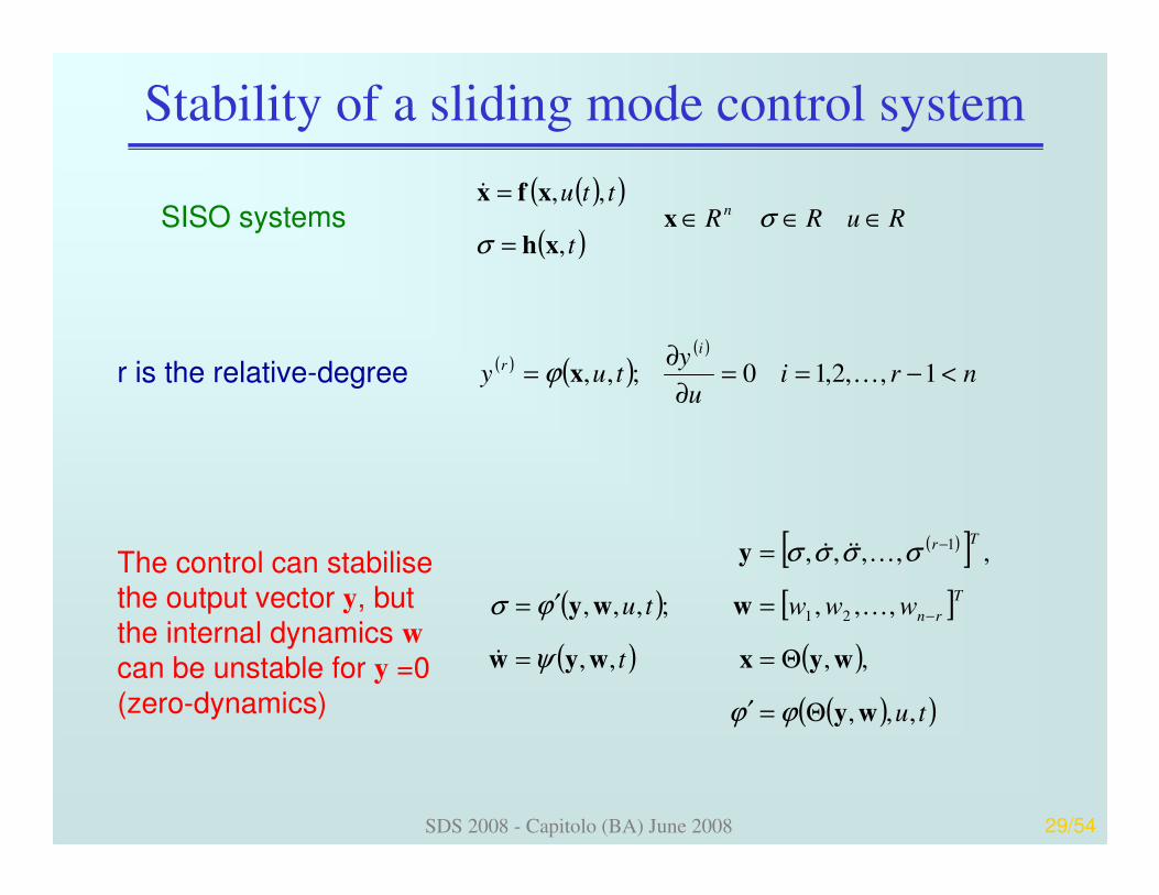
Stability of a sliding mode control system
SISO systems( )( )
( )RuRR
t
ttun ∈∈∈
=
=σ
σx
xh
xfx
,
,,&
( ) ( )( )
nriu
ytuy
ir <−==
∂
∂= 1,,2,10;,, Kxϕr is the relative-degree
( )[ ]( ) [ ]
( ) ( )
( )( )tu
t
wwwtuT
rn
Tr
,,,
,,,,
,,,;,,,
,,,,,
21
1
wy
wyxwyw
wwy
y
Θ=′
Θ==
=′=
=
−
−
ϕϕ
ψ
ϕσ
σσσσ
&
K
K&&&The control can stabilise the output vector y, but the internal dynamics wcan be unstable for y =0
(zero-dynamics)
SDS 2008 - Capitolo (BA) June 2008 30/54
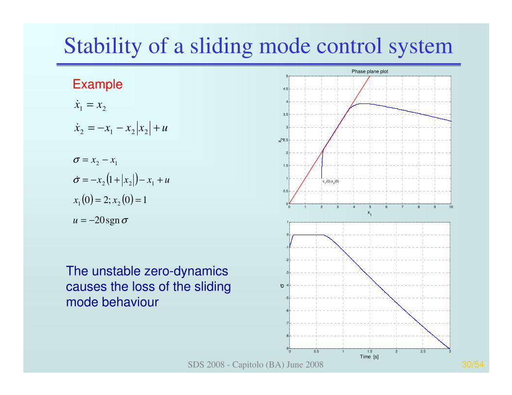
Stability of a sliding mode control system
2212
21
uxxxx
xx
+−−=
=
&
&
( )
( ) ( )
σ
σ
σ
sgn20
10;20
1
21
122
12
−=
==
+−+−=
−=
u
xx
uxxx
xx
&
Example
0 1 2 3 4 5 6 7 8 9 100
0.5
1
1.5
2
2.5
3
3.5
4
4.5
5
Phase plane plot
x1
x 2
x1(0);x
2(0)
0 0.5 1 1.5 2 2.5 3-9
-8
-7
-6
-5
-4
-3
-2
-1
0
1
Time [s]
σ
The unstable zero-dynamics causes the loss of the sliding mode behaviour
SDS 2008 - Capitolo (BA) June 2008 31/54
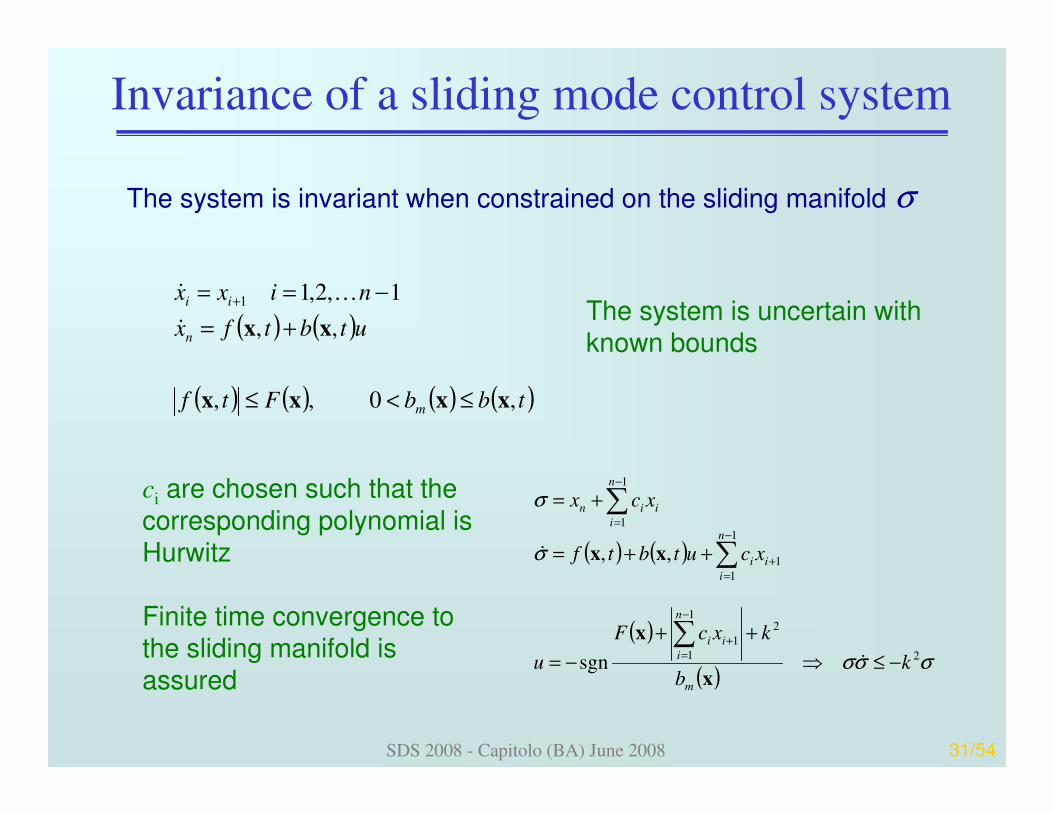
Invariance of a sliding mode control system
( ) ( )
( ) ( ) ( ) ( )tbbFtf
utbtfx
nixx
m
n
ii
,0,,
,,
1,2,11
xxxx
xx
≤<≤
+=
−== +
&
K&
The system is invariant when constrained on the sliding manifold σ
( ) ( )
( )
( )σσσ
σ
σ
2
21
1
1
1
1
1
1
1
sgn
,,
kb
kxcF
u
xcutbtf
xcx
m
n
i
ii
n
i
ii
n
i
iin
−≤⇒
++
−=
++=
+=
∑
∑
∑
−
=+
−
=+
−
=
&
&
x
x
xx
The system is uncertain with known bounds
ci are chosen such that the
corresponding polynomial is Hurwitz
Finite time convergence to the sliding manifold is assured

SDS 2008 - Capitolo (BA) June 2008 32/54
Invariance of a sliding mode control system
The system is invariant when constrained on the sliding manifold σ
∑
∑−
=
−
=−
+
+−=
+−=
−==
1
1
1
1
1
1 2,2,1
n
i
iin
n
i
iin
ii
xcx
xcx
nixx
σ
σ&
K&
The system behaves as a reduced order system with prescribed eigenvalues
Matching uncertainties, included in the uncertain function f, are
completely rejected
In the sliding mode it is not possible to “recover” the original system dynamics (semi-group property)
Take care of unstable zero-dynamics
SDS 2008 - Capitolo (BA) June 2008 33/54
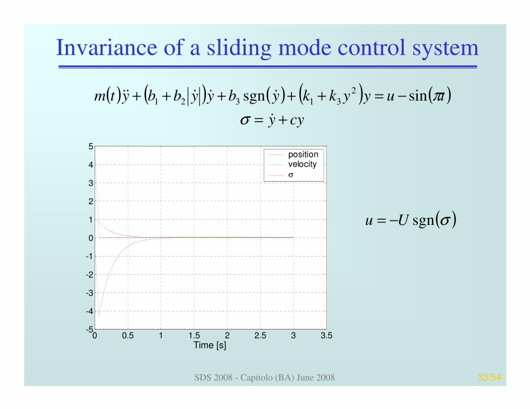
Invariance of a sliding mode control system
( ) ( ) ( ) ( ) ( )cyy
tuyykkybyybbytm
+=
−=+++++
&
&&&&&
σ
πsinsgn 2
31321
( )σsgnUu −=
0 0.5 1 1.5 2 2.5 3 3.5-5
-4
-3
-2
-1
0
1
2
3
4
5
Time [s]
positionvelocity
σ

SDS 2008 - Capitolo (BA) June 2008 34/54
Invariance of a sliding mode control system
SystemVSCref. +
_
σ u y
SystemInternal
Model
ueq yd
+ +d
+ +d
The invariance property during the sliding mode means that the “Internal Model Principle” is fulfilled

SDS 2008 - Capitolo (BA) June 2008 35/54
Invariance of a sliding mode control system
( ) ( )[ ]UUtbtf +−+=∈ ,,, xxx F&
The controlled system dynamics belongs to a differential inclusion
The sliding variable σ can be considered as a performance index to be nullified to find the “right” solution
( ) ( ) F∈+= equtbtf ,,* xxx&
SDS 2008 - Capitolo (BA) June 2008 36/54
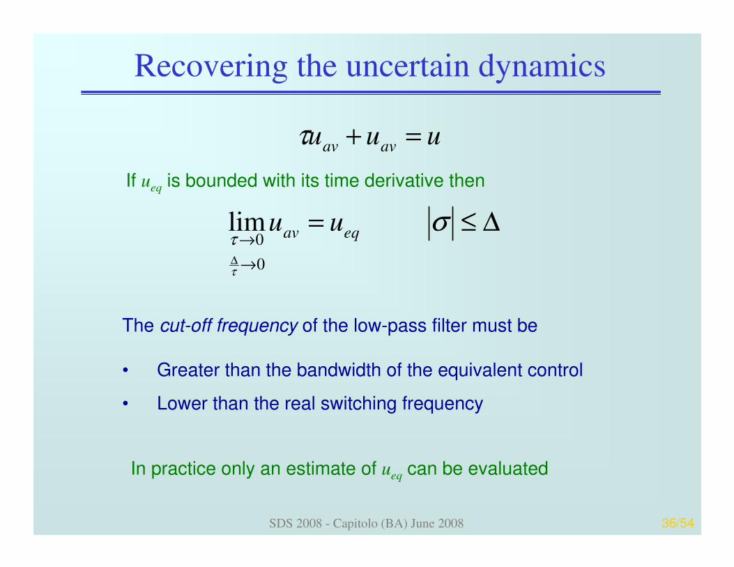
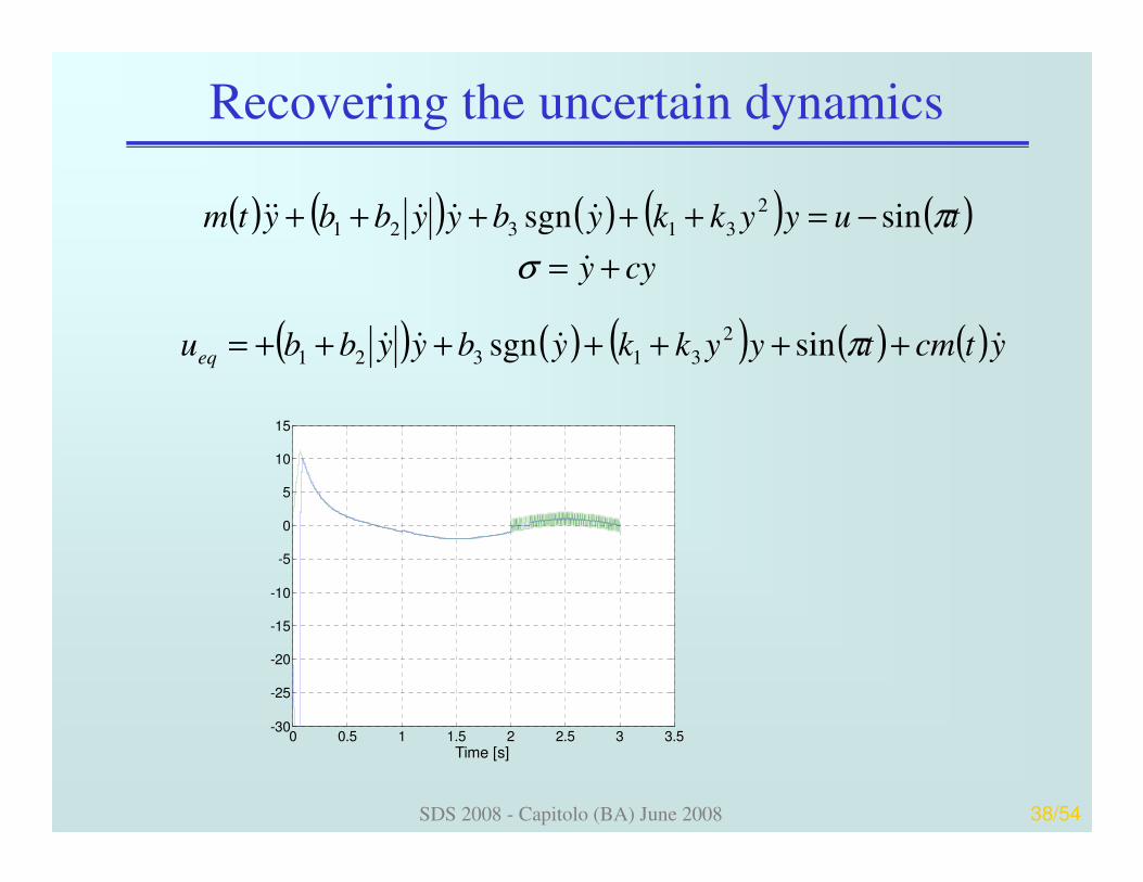
Recovering the uncertain dynamics
uuu avav =+τ
If ueq is bounded with its time derivative then
∆≤=
→
→∆
σ
τ
τ eqav uu
0
0lim
The cut-off frequency of the low-pass filter must be
• Greater than the bandwidth of the equivalent control
• Lower than the real switching frequency
In practice only an estimate of ueq can be evaluated
SDS 2008 - Capitolo (BA) June 2008 37/54
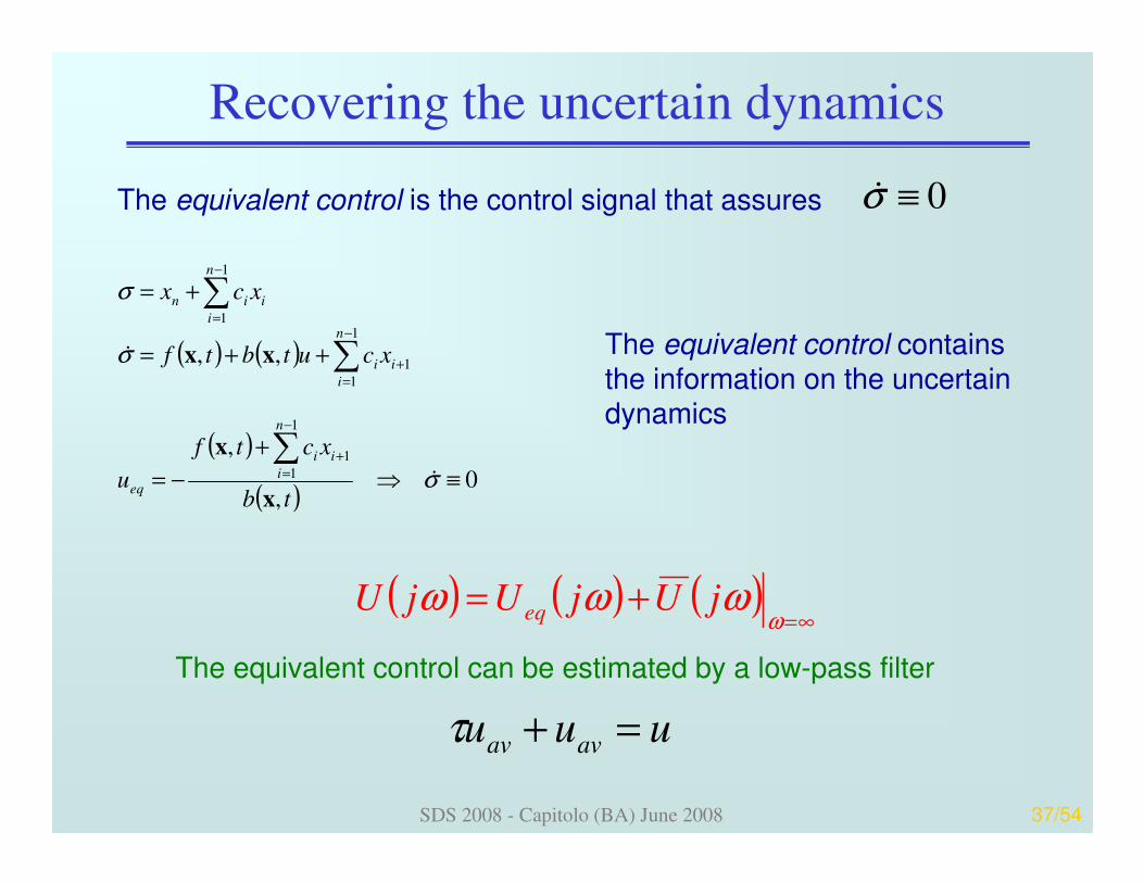
Recovering the uncertain dynamics
The equivalent control is the control signal that assures 0≡σ&
( ) ( )
( )
( )0
,
,
,,
1
1
1
1
1
1
1
1
≡⇒
+
−=
++=
+=
∑
∑
∑
−
=+
−
=+
−
=
σ
σ
σ
&
&
tb
xctf
u
xcutbtf
xcx
n
i
ii
eq
n
i
ii
n
i
iin
x
x
xx The equivalent control contains the information on the uncertain dynamics
( ) ( ) ( )∞=
+=ω
ωωω jUjUjU eq
The equivalent control can be estimated by a low-pass filter
uuu avav =+τ
SDS 2008 - Capitolo (BA) June 2008 38/54
Recovering the uncertain dynamics
( ) ( ) ( ) ( ) ( )cyy
tuyykkybyybbytm
+=
−=+++++
&
&&&&&
σ
πsinsgn 2
31321
( ) ( ) ( ) ( ) ( )ytcmtyykkybyybbueq&&&& +++++++= πsinsgn
2
31321
0 0.5 1 1.5 2 2.5 3 3.5-30
-25
-20
-15
-10
-5
0
5
10
15
Time [s]

SDS 2008 - Capitolo (BA) June 2008 39/54
Approximability
∑
∑−
=
−
=−
+
+−=
+−=
−==
1
1
1
1
1
1 2,2,1
n
i
iin
n
i
iin
ii
xcx
xcx
nixx
σ
σ&
K&
The dynamics of the original system can be reduced to
In the case of switching errors – the switching frequency is fs≤∞ –the real trajectory x(t) is near to the ideal one x*(t) and
( ) ( ) 0* →−→∞sf
tt xx
( ) ( )[ ]( ) ( ) ( ) xxxx
xxx
NMtutbtf
UUtbtf
+≤+
+−+=
,,,
,,,&Assuming that the dynamics of the original system is bounded
SDS 2008 - Capitolo (BA) June 2008 40/54
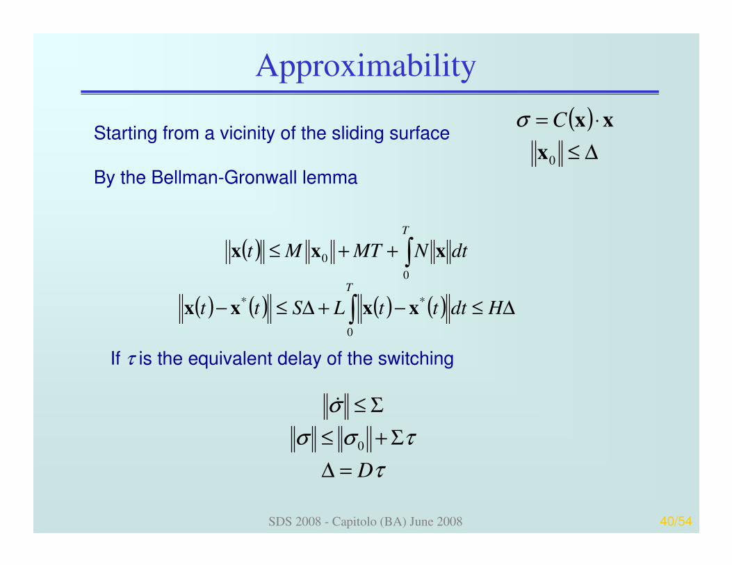
Approximability
( )∆≤
⋅=
0x
xxCσStarting from a vicinity of the sliding surface
By the Bellman-Gronwall lemma
( )
( ) ( ) ( ) ( ) ∆≤−+∆≤−
++≤
∫
∫
HdtttLStt
dtNMTMt
T
T
0
**
0
0
xxxx
xxx
τ
τσσ
σ
D=∆
Σ+≤
Σ≤
0
&
If τ is the equivalent delay of the switching
SDS 2008 - Capitolo (BA) June 2008 41/54
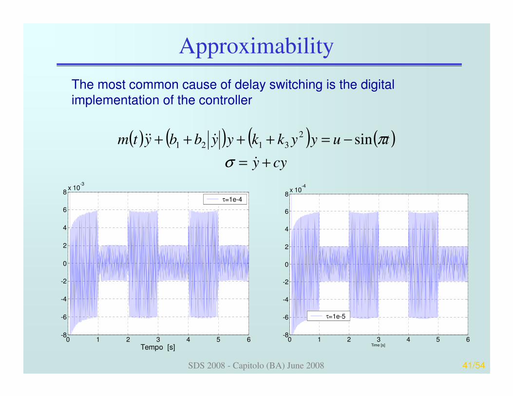
Approximability
The most common cause of delay switching is the digital implementation of the controller
0 1 2 3 4 5 6-8
-6
-4
-2
0
2
4
6
8x 10
-3
Tempo [s]
τ=1e-4
( ) ( ) ( ) ( )cyy
tuyykkyybbytm
+=
−=++++
&
&&&
σ
πsin2
3121
0 1 2 3 4 5 6-8
-6
-4
-2
0
2
4
6
8x 10
-4
Time [s]
τ=1e-5
SDS 2008 - Capitolo (BA) June 2008 42/54
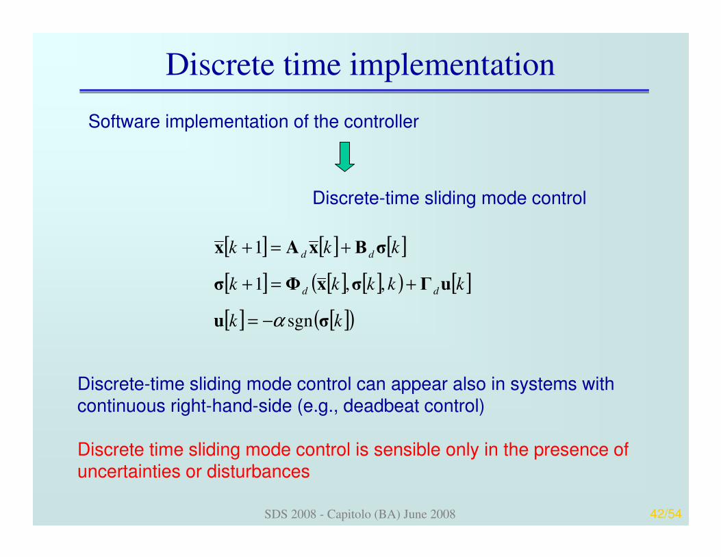
Discrete time implementation
Software implementation of the controller
Discrete-time sliding mode control
[ ] [ ] [ ]
[ ] [ ] [ ]( ) [ ]
[ ] [ ]( )kk
kkkkk
kkk
dd
dd
σu
uΓσxΦσ
σΒxAx
sgn
,,1
1
α−=
+=+
+=+
Discrete-time sliding mode control can appear also in systems with continuous right-hand-side (e.g., deadbeat control)
Discrete time sliding mode control is sensible only in the presence of uncertainties or disturbances
SDS 2008 - Capitolo (BA) June 2008 43/54
Discrete time implementation
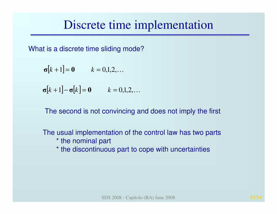
[ ] K,2,1,01 ==+ kk 0σ
What is a discrete time sliding mode?
[ ] [ ] K,2,1,01 ==−+ kkk 0σσ
The second is not convincing and does not imply the first
The usual implementation of the control law has two parts* the nominal part* the discontinuous part to cope with uncertainties
SDS 2008 - Capitolo (BA) June 2008 44/54
Discrete time implementation
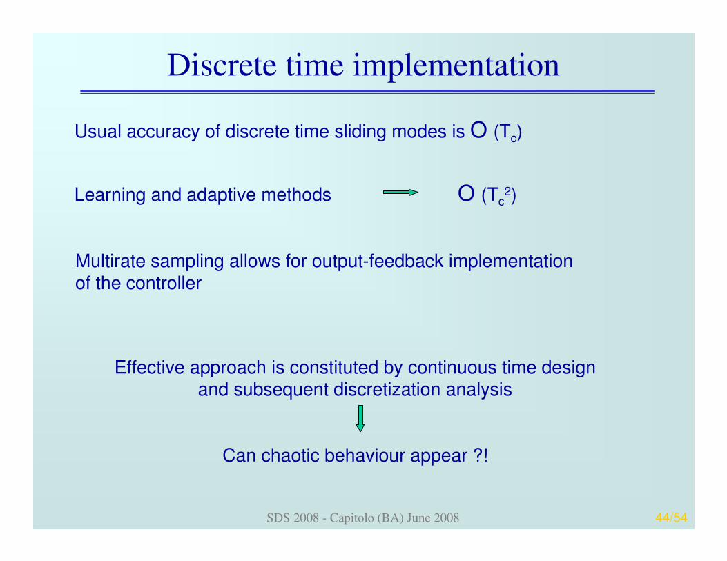
Usual accuracy of discrete time sliding modes is O (Tc)
Learning and adaptive methods O (Tc2)
Multirate sampling allows for output-feedback implementation of the controller
Effective approach is constituted by continuous time design and subsequent discretization analysis
Can chaotic behaviour appear ?!

SDS 2008 - Capitolo (BA) June 2008 45/54
Higher order sliding modes
The sliding mode concept can be extended to more complete integral manifolds
( ) 01 ===== −rσσσσ L&&&
r constraints are introduced in the system dynamics
The control acts on the r-th derivative of the sliding
variable σ
Accuracy is improved
( ) 1,,2,1,0, −== −riH
ir
i
iKτσ
Hi does not depend on τ

SDS 2008 - Capitolo (BA) June 2008 46/54
Higher order sliding modes
The internal dynamics has a reduced dimension n-r
The robustness properties are preserved
The approximability property is preserved
Allows for chattering attenuation
No general Lyapunov-like methods for the stability analysis are available (only very recent results for r=2 were presented)
Phase plane of homogeneity approaches to state the closed-loop stability
Derivatives of the sliding variable σ are needed
SDS 2008 - Capitolo (BA) June 2008 47/54
Higher order sliding modes
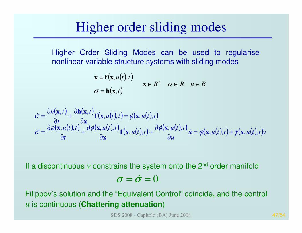
Higher Order Sliding Modes can be used to regularise nonlinear variable structure systems with sliding modes
( )( )
( )RuRR
t
ttun ∈∈∈
=
=σ
σx
xh
xfx
,
,,&
( ) ( ) ( )( ) ( )( )
( )( ) ( )( ) ( )( ) ( )( ) ( )( ) ( )( )vttuttuuu
ttuttu
ttu
t
ttu
ttuttut
t
th
,,,,,,
,,,,,,
,,,,,,
xxx
xfx
xx
xxfx
xhx
γϕφφφ
σ
φσ
+=∂
∂+
∂
∂+
∂
∂=
=∂
∂+
∂
∂=
&&&
&
If a discontinuous v constrains the system onto the 2nd order manifold
Filippov’s solution and the “Equivalent Control” coincide, and the control
u is continuous (Chattering attenuation)
0== σσ &
SDS 2008 - Capitolo (BA) June 2008 48/54
Higher order sliding modes
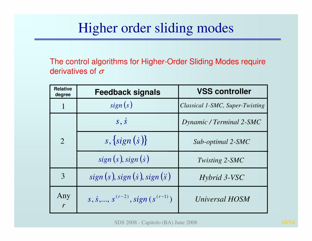
The control algorithms for Higher-Order Sliding Modes require
derivatives of σ
Relativedegree Feedback signals VSS controller
1 Classical 1-SMC, Super-Twisting( )ssign
2
( ) ( )ssignssign &, Twisting 2-SMC
( ) ssigns &, Sub-optimal 2-SMC
3
ss &,
Any
rUniversal HOSM )(,,...,, )1()2( −− rr ssignsss &
( ) ( ) ( )ssignssignssign &&& ,, Hybrid 3-VSC
Dynamic / Terminal 2-SMC
SDS 2008 - Capitolo (BA) June 2008 49/54
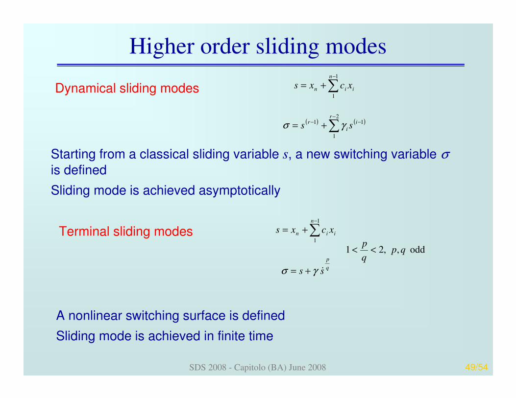
Higher order sliding modes
Dynamical sliding modes
( ) ( )∑
∑
−−−
−
+=
+=
2
1
11
1
1
ri
i
r
n
iin
ss
xcxs
γσ
Starting from a classical sliding variable s, a new switching variable σis defined
Sliding mode is achieved asymptotically
Terminal sliding modes
odd , ,21
1
1
qpq
p
ss
xcxs
q
p
n
iin
<<
+=
+= ∑−
&γσ
A nonlinear switching surface is defined
Sliding mode is achieved in finite time
SDS 2008 - Capitolo (BA) June 2008 50/54
Higher order sliding modes
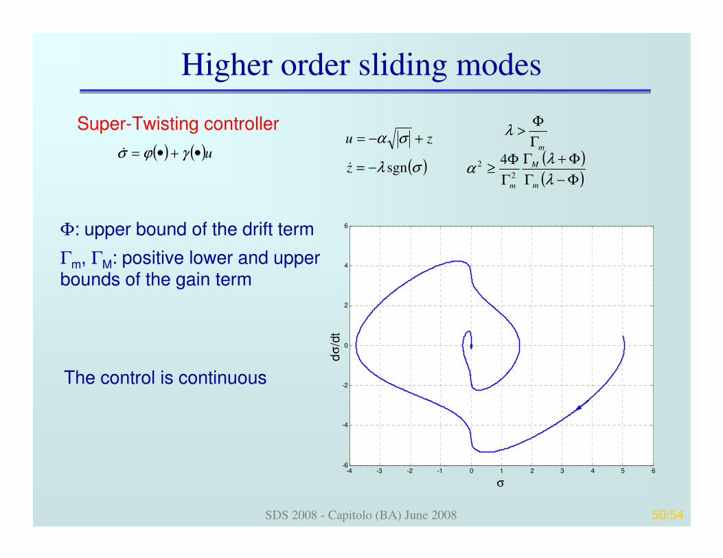
Super-Twisting controller
( ) ( )( )Φ−Γ
Φ+Γ
Γ
Φ≥
Γ
Φ>
−=
+−=
λ
λα
λ
σλ
σα
m
M
m
m
z
zu
2
2 4sgn&
Φ: upper bound of the drift term
Γm, ΓM: positive lower and upper bounds of the gain term
-4 -3 -2 -1 0 1 2 3 4 5 6-6
-4
-2
0
2
4
6
σ
dσ
/dt
The control is continuous
( ) ( )u•+•= γϕσ&
SDS 2008 - Capitolo (BA) June 2008 51/54
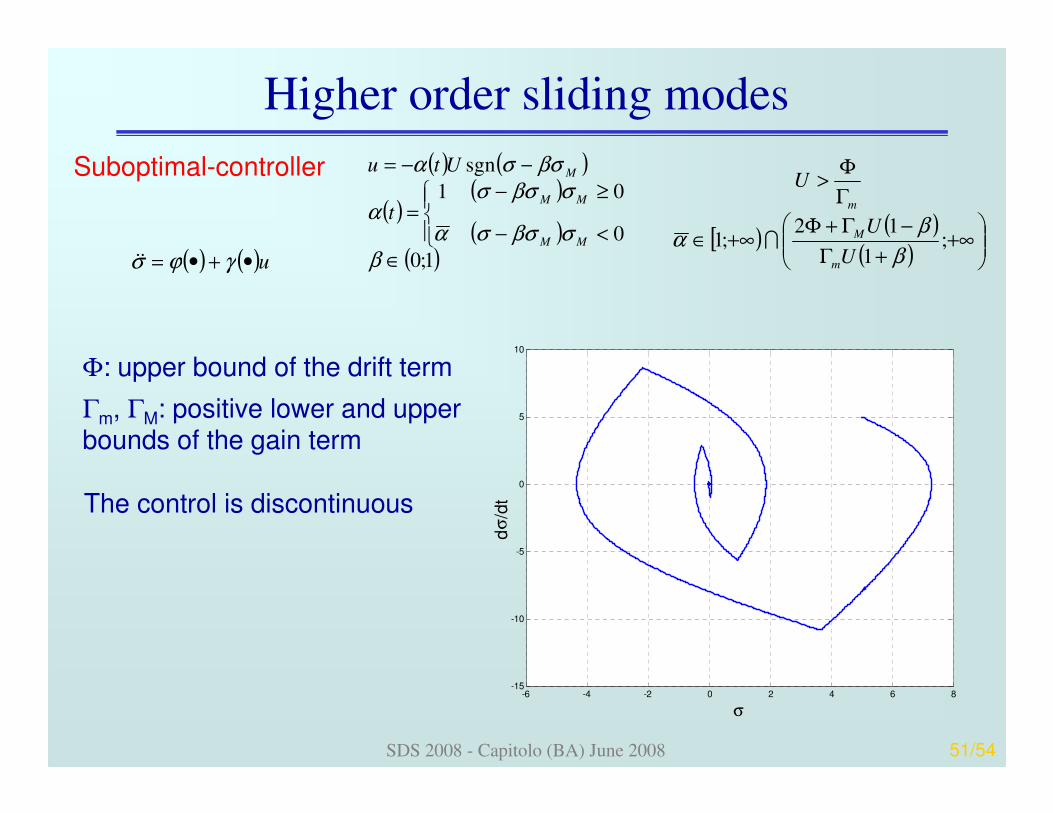
Higher order sliding modes
Suboptimal-controller ( ) ( )
( )( )
( )( )
[ )( )
( )
+∞
+Γ
−Γ+Φ+∞∈
Γ
Φ>
∈
<−
≥−=
−−=
;1
12;1
1;0
0
01
sgn
β
βα
βσβσσα
σβσσα
βσσα
U
U
U
t
Utu
m
M
m
MM
MM
M
I
Φ: upper bound of the drift term
Γm, ΓM: positive lower and upper bounds of the gain term
The control is discontinuous
( ) ( )u•+•= γϕσ&&
-6 -4 -2 0 2 4 6 8-15
-10
-5
0
5
10
σ
dσ
/dt
SDS 2008 - Capitolo (BA) June 2008 52/54
Higher order sliding modes
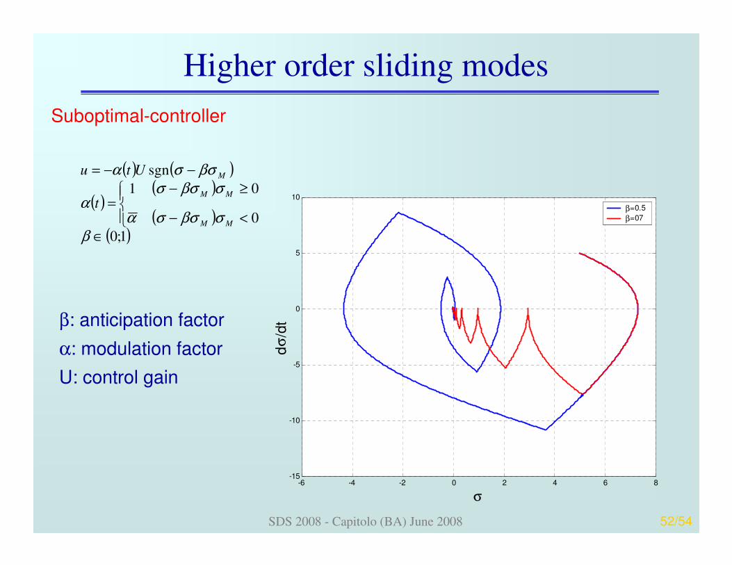
Suboptimal-controller
β: anticipation factor
α: modulation factor
U: control gain
-6 -4 -2 0 2 4 6 8-15
-10
-5
0
5
10
σ
dσ
/dt
β=0.5
β=07
( ) ( )
( )( )
( )( )1;0
0
01
sgn
∈
<−
≥−=
−−=
βσβσσα
σβσσα
βσσα
MM
MM
M
t
Utu
SDS 2008 - Capitolo (BA) June 2008 53/54
Higher order sliding modes
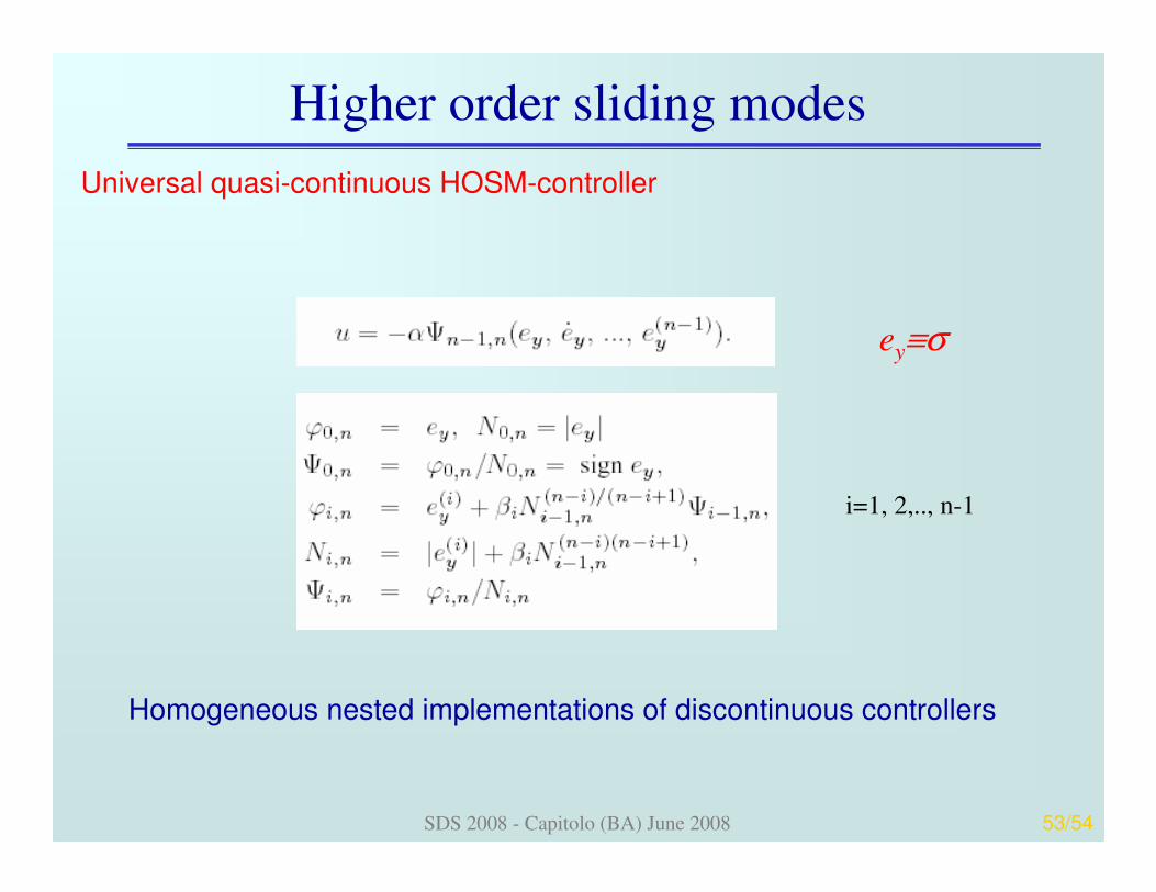
Universal quasi-continuous HOSM-controller
i=1, 2,.., n-1
Homogeneous nested implementations of discontinuous controllers
ey≡σ
SDS 2008 - Capitolo (BA) June 2008 54/54
Final remarks
Sliding Modes are a usual behaviour in switching systems
Sliding Modes are a useful tool for controlling uncertain dynamical systems
Switching control with Sliding Modes is a simple way of applying the Internal Model Principle
By resorting to the Equivalent Control definition it is possible to retrieve some information about an uncertain system by low-pass filters
Ideal Sliding Modes are not implemented in practice because theyrequire infinite frequency switching, and only an approximate sliding can be achieved
Higher Order Sliding Modes generalise the concept of sliding modes to integral manifolds
Real Higher Order Sliding Modes improve the accuracy and attenuate the chattering effect