slide 1 of 82 linear programming: transportation problem j. loucks, st. edward's university...
TRANSCRIPT

Slide 1 of 82 Slide 1 of 82
Linear Programming: Transportation Linear Programming: Transportation ProblemProblem
J. Loucks, St. Edward's University (Austin, TX, USA)
Chapter 2BChapter 2B

Slide 2 of 82 Slide 2 of 82
A A network modelnetwork model is one which can be is one which can be represented by a set of nodes, a set of arcs, represented by a set of nodes, a set of arcs, and functions (e.g. costs, supplies, demands, and functions (e.g. costs, supplies, demands, etc.) associated with the arcs and/or nodes.etc.) associated with the arcs and/or nodes.
Transportation problem (TP), as well as many Transportation problem (TP), as well as many other problems, are all examples of network other problems, are all examples of network problems.problems.
Efficient solution algorithms exist to solve Efficient solution algorithms exist to solve network problems. network problems.
Transportation ProblemTransportation Problem
Slide 3 of 82 Slide 3 of 82
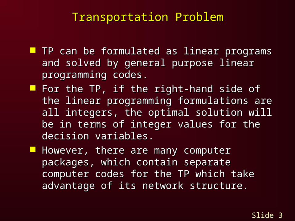
TP can be formulated as linear programs and TP can be formulated as linear programs and solved by general purpose linear programming solved by general purpose linear programming codes. codes.
For the TP, if the right-hand side of the linear For the TP, if the right-hand side of the linear programming formulations are all integers, the programming formulations are all integers, the optimal solution will be in terms of integer optimal solution will be in terms of integer values for the decision variables.values for the decision variables.
However, there are many computer packages, However, there are many computer packages, which contain separate computer codes for the which contain separate computer codes for the TP which take advantage of its network TP which take advantage of its network structure.structure.
Transportation ProblemTransportation Problem

Slide 4 of 82 Slide 4 of 82
Transportation ProblemTransportation Problem
The TP problem has the following characteristics:The TP problem has the following characteristics:• mm sources and sources and nn destinations destinations• number of variables is m x nnumber of variables is m x n• number of constraints is m + n (constraints number of constraints is m + n (constraints
are for source capacity and destination are for source capacity and destination demand)demand)
• costs appear only in objective function costs appear only in objective function (objective is to minimize total cost of shipping)(objective is to minimize total cost of shipping)
• coefficients of decision variables in the coefficients of decision variables in the constraints are either 0 or 1constraints are either 0 or 1

Slide 5 of 82 Slide 5 of 82
The The transportation problemtransportation problem seeks to minimize seeks to minimize the total shipping costs of transporting goods the total shipping costs of transporting goods from from mm origins (each with a supply origins (each with a supply ssii) to ) to nn destinations (each with a demand destinations (each with a demand ddjj), when ), when the unit shipping cost from an origin, the unit shipping cost from an origin, ii, to a , to a destination, destination, jj, is , is ccijij..
The The network representationnetwork representation for a for a transportation problem with two sources and transportation problem with two sources and three destinations is given on the next slide.three destinations is given on the next slide.
Transportation ProblemTransportation Problem

Slide 6 of 82 Slide 6 of 82
Transportation ProblemTransportation Problem
Network RepresentationNetwork Representation
11
22
33
11
22
cc1111
cc1212
cc1313
cc2121 cc2222
cc2323
dd11
dd22
dd33
ss11
s2
SOURCESSOURCES DESTINATIONSDESTINATIONS

Slide 7 of 82 Slide 7 of 82
The Relationship of TP to LPThe Relationship of TP to LP
TP is a special case of LPTP is a special case of LP How do we formulate TP as an LP?How do we formulate TP as an LP?
• Let xLet xijij = quantity of product shipped from = quantity of product shipped from source i to destination jsource i to destination j
• Let cLet cijij = per unit shipping cost from source i to = per unit shipping cost from source i to destination jdestination j
• Let sLet sii be the row i total supply be the row i total supply
• Let dLet djj be the column j total demand be the column j total demand The LP formulation of the TP problem is:The LP formulation of the TP problem is:

Slide 8 of 82 Slide 8 of 82
LP FormulationLP Formulation
The linear programming formulation in terms of The linear programming formulation in terms of the amounts shipped from the origins to the the amounts shipped from the origins to the destinations, destinations, xxijij, can be written as:, can be written as:
Min Min ccijijxxijij
i ji j
s.t. s.t. xxijij << ssii for each origin for each origin ii jj
xxijij >> ddjj for each destination for each destination jj ii
xxijij >> 0 for all 0 for all ii and and jj
The Relationship of TP to LPThe Relationship of TP to LP

Slide 9 of 82 Slide 9 of 82
Transportation ProblemTransportation Problem
LP Formulation Special CasesLP Formulation Special Cases
The following special-case modifications to the The following special-case modifications to the linear programming formulation can be made:linear programming formulation can be made:• Minimum shipping guarantees from Minimum shipping guarantees from ii to to jj: :
xxijij >> LLijij
• Maximum route capacity from Maximum route capacity from ii to to jj::
xxijij << LLijij
• Unacceptable routes: Unacceptable routes:
delete the variable (or put a very high cost, delete the variable (or put a very high cost, called the Big-M method, on a selected pair of called the Big-M method, on a selected pair of i and j)i and j)

Slide 10 of 82 Slide 10 of 82
To solve the transportation problem by its special To solve the transportation problem by its special purpose algorithm, it is required that the sum of purpose algorithm, it is required that the sum of the supplies at the origins equal the sum of the the supplies at the origins equal the sum of the demands at the destinations. If the total supply demands at the destinations. If the total supply is greater than the total demand, a dummy is greater than the total demand, a dummy destination is added with demand equal to the destination is added with demand equal to the excess supply, and shipping costs from all origins excess supply, and shipping costs from all origins are zero. Similarly, if total supply is less than are zero. Similarly, if total supply is less than total demand, a dummy origin is added. total demand, a dummy origin is added.
When solving a transportation problem by its When solving a transportation problem by its special purpose algorithm, unacceptable shipping special purpose algorithm, unacceptable shipping routes are given a cost of +routes are given a cost of +MM (a large number). (a large number).
Transportation ProblemTransportation Problem

Slide 11 of 82 Slide 11 of 82
The transportation problem is solved in two The transportation problem is solved in two phases: phases: • Phase I — Obtaining an initial feasible solutionPhase I — Obtaining an initial feasible solution• Phase II — Moving toward optimalityPhase II — Moving toward optimality
In Phase I, the Minimum-Cost Procedure can be In Phase I, the Minimum-Cost Procedure can be used to establish an initial basic feasible solution used to establish an initial basic feasible solution without doing numerous iterations of the simplex without doing numerous iterations of the simplex method.method.
In Phase II, the Stepping Stone Method, using the In Phase II, the Stepping Stone Method, using the MODI method for evaluating the reduced costs MODI method for evaluating the reduced costs may be used to move from the initial feasible may be used to move from the initial feasible solution to the optimal one.solution to the optimal one.
Transportation ProblemTransportation Problem

Slide 12 of 82 Slide 12 of 82
Phase I - Minimum-Cost Method (simple and Phase I - Minimum-Cost Method (simple and intuitive)intuitive)• Step 1: Step 1: Select the cell with the least cost. Select the cell with the least cost.
Assign to this cell the minimum of its remaining Assign to this cell the minimum of its remaining row supply or remaining column demand.row supply or remaining column demand.
• Step 2: Step 2: Decrease the row and column Decrease the row and column availabilities by this amount and remove from availabilities by this amount and remove from consideration all other cells in the row or consideration all other cells in the row or column with zero availability/demand. (If both column with zero availability/demand. (If both are simultaneously reduced to 0, assign an are simultaneously reduced to 0, assign an allocation of 0 to any other unoccupied cell in allocation of 0 to any other unoccupied cell in the row or column before deleting both.) GO TO the row or column before deleting both.) GO TO STEP 1.STEP 1.
Transportation AlgorithmTransportation Algorithm

Slide 13 of 82 Slide 13 of 82
Transportation AlgorithmTransportation Algorithm
Phase II - Stepping Stone MethodPhase II - Stepping Stone Method• Step 1: Step 1: For each unoccupied cell, calculate the For each unoccupied cell, calculate the
reduced cost by the MODI method described reduced cost by the MODI method described below. below. Select the unoccupied cell with Select the unoccupied cell with the most negative reduced cost. (For the most negative reduced cost. (For maximization problems select the unoccupied cell maximization problems select the unoccupied cell with the largest reduced cost.) If none, STOP.with the largest reduced cost.) If none, STOP.
• Step 2: Step 2: For this unoccupied cell generate a For this unoccupied cell generate a stepping stone path by forming a closed loop with stepping stone path by forming a closed loop with this cell and occupied cells by drawing connecting this cell and occupied cells by drawing connecting alternating horizontal and vertical lines between alternating horizontal and vertical lines between them. them.
Determine the minimum allocation Determine the minimum allocation where a subtraction is to be made along this path. where a subtraction is to be made along this path.

Slide 14 of 82 Slide 14 of 82
Transportation AlgorithmTransportation Algorithm
Phase II - Stepping Stone Method (continued)Phase II - Stepping Stone Method (continued)• Step 3: Step 3: Add this allocation to all cells where Add this allocation to all cells where
additions are to be made, and subtract this additions are to be made, and subtract this allocation to all cells where subtractions are to allocation to all cells where subtractions are to be made along the stepping stone path. be made along the stepping stone path. (Note: An occupied cell on the stepping stone (Note: An occupied cell on the stepping stone path now becomes 0 (unoccupied). path now becomes 0 (unoccupied).
If more than one cell becomes 0, If more than one cell becomes 0, make only one unoccupied; make the others make only one unoccupied; make the others occupied with 0's.) GO TO STEP 1.occupied with 0's.) GO TO STEP 1.

Slide 15 of 82 Slide 15 of 82
Transportation AlgorithmTransportation Algorithm
MODI Method (for obtaining reduced costs)MODI Method (for obtaining reduced costs)
Associate a number, Associate a number, uuii, with each row and , with each row and vvjj with each column. with each column.
• Step 1: Step 1: Set Set uu11 = 0. = 0.
• Step 2: Step 2: Calculate the remaining Calculate the remaining uuii's and 's and vvjj's 's by solving the relationship by solving the relationship ccijij = = uuii + + vvjj for for occupied cells.occupied cells.
• Step 3: Step 3: For unoccupied cells (For unoccupied cells (ii,,jj), the reduced ), the reduced cost = cost = ccijij - - uuii - - vvjj..

Slide 16 of 82 Slide 16 of 82
A A transportation tableautransportation tableau is given below. Each is given below. Each cell represents a shipping route (which is an cell represents a shipping route (which is an arc on the network and a decision variable in arc on the network and a decision variable in the LP formulation), and the unit shipping the LP formulation), and the unit shipping costs are given in an upper right hand box in costs are given in an upper right hand box in the cell. the cell.
SupplySupply
3030
5050
35353535
20202020
40404040
30303030
30303030
DemandDemand 101045452525
S1S1
S2S2
D3D3D2D2D1D1
15151515
Example 1: TPExample 1: TP

Slide 17 of 82 Slide 17 of 82
Example 1: TPExample 1: TP
Building Brick Company (BBC) has orders for Building Brick Company (BBC) has orders for 80 tons of bricks at three suburban locations as 80 tons of bricks at three suburban locations as follows: Northwood — 25 tons, Westwood — 45 follows: Northwood — 25 tons, Westwood — 45 tons, and Eastwood — 10 tons. BBC has two plants, tons, and Eastwood — 10 tons. BBC has two plants, each of which can produce 50 tons per week. each of which can produce 50 tons per week.
How should end of week shipments be made How should end of week shipments be made to fill the above orders given the following delivery to fill the above orders given the following delivery cost per ton:cost per ton:
NorthwoodNorthwood WestwoodWestwood EastwoodEastwood
Plant 1 24 Plant 1 24 30 30 4040
Plant 2 Plant 2 30 30 40 40 42 42

Slide 18 of 82 Slide 18 of 82
Example 1: TPExample 1: TP
Initial Transportation TableauInitial Transportation Tableau
Since total supply = 100 and total demand Since total supply = 100 and total demand = 80, a dummy destination is created with = 80, a dummy destination is created with demand of 20 and 0 unit costs.demand of 20 and 0 unit costs.
42424242
40404040 0000
000040404040
30303030
30303030
DemandDemand
SupplySupply
5050
5050
2020101045452525
DummyDummy
Plant 1Plant 1
Plant 2Plant 2
EastwoodEastwoodWestwoodWestwoodNorthwoodNorthwood
24242424

Slide 19 of 82 Slide 19 of 82
Example 1: TPExample 1: TP
Least Cost Starting ProcedureLeast Cost Starting Procedure• Iteration 1: Iteration 1: Tie for least cost (0), arbitrarily Tie for least cost (0), arbitrarily
select select xx1414. Allocate 20. Reduce . Allocate 20. Reduce ss11 by 20 to 30 by 20 to 30 and delete the Dummy column.and delete the Dummy column.
• Iteration 2: Iteration 2: Of the remaining cells the least Of the remaining cells the least cost is 24 for cost is 24 for xx1111. Allocate 25. Reduce . Allocate 25. Reduce ss11 by by 25 to 5 and eliminate the Northwood column.25 to 5 and eliminate the Northwood column.
• Iteration 3: Iteration 3: Of the remaining cells the least Of the remaining cells the least cost is 30 for cost is 30 for xx1212. Allocate 5. Reduce the . Allocate 5. Reduce the Westwood column to 40 and eliminate the Westwood column to 40 and eliminate the Plant 1 row.Plant 1 row.
• Iteration 4: Iteration 4: Since there is only one row with Since there is only one row with two cells left, make the final allocations of 40 two cells left, make the final allocations of 40 and 10 to and 10 to xx2222 and and xx2323, respectively., respectively.

Slide 20 of 82 Slide 20 of 82
Example 1: TPExample 1: TP
Iteration 1Iteration 1• MODI MethodMODI Method
1. Set 1. Set uu11 = 0 = 0
2. Since 2. Since uu11 + + vvjj = = cc11jj for occupied cells in for occupied cells in row 1, thenrow 1, then
vv11 = 24, = 24, vv22 = 30, = 30, vv44 = 0. = 0.
3. Since 3. Since uuii + + vv22 = = ccii22 for occupied cells in for occupied cells in column 2, column 2, then then uu22 + 30 = 40, hence + 30 = 40, hence uu22 = 10. = 10.
4. Since 4. Since uu22 + + vvjj = = cc22jj for occupied cells in for occupied cells in row 2, thenrow 2, then
10 + 10 + vv33 = 42, hence = 42, hence vv33 = 32. = 32.
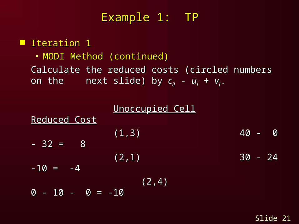
Slide 21 of 82 Slide 21 of 82
Example 1: TPExample 1: TP
Iteration 1Iteration 1• MODI Method (continued)MODI Method (continued)
Calculate the reduced costs (circled Calculate the reduced costs (circled numbers on the numbers on the next slide) by next slide) by ccijij - - uuii + + vvjj..
Unoccupied CellUnoccupied Cell Reduced CostReduced Cost
(1,3) 40 - 0 - 32 = (1,3) 40 - 0 - 32 = 88
(2,1) 30 - 24 -10 = -(2,1) 30 - 24 -10 = -44
(2,4) 0 - 10 - 0 = -(2,4) 0 - 10 - 0 = -1010

Slide 22 of 82 Slide 22 of 82
Example 1: TPExample 1: TP
Iteration 1 TableauIteration 1 Tableau
2525 2525 5 5 5 5
-4 -4 -4 -4
+8 +8 +8 +8 20 20 20 20
40 40 40 40 10 10 10 10 -10 -10 -10 -10 42424242
40404040 0000
000040404040
30303030
30303030
vvjj
uuii
1010
00
00323230302424
DummyDummy
Plant 1Plant 1
Plant 2Plant 2
EastwoodEastwoodWestwoodWestwoodNorthwoodNorthwood
24242424

Slide 23 of 82 Slide 23 of 82
Example 1: TPExample 1: TP
Iteration 1Iteration 1• Stepping Stone MethodStepping Stone Method
The stepping stone path for cell (2,4) is (2,4), The stepping stone path for cell (2,4) is (2,4), (1,4), (1,2), (2,2). The allocations in the subtraction (1,4), (1,2), (2,2). The allocations in the subtraction cells are 20 and 40, respectively. The minimum is cells are 20 and 40, respectively. The minimum is 20, and hence reallocate 20 along this path. Thus for 20, and hence reallocate 20 along this path. Thus for the next tableau:the next tableau:
xx2424 = 0 + 20 = 20 (0 is its current allocation) = 0 + 20 = 20 (0 is its current allocation)
xx1414 = 20 - 20 = 0 (blank for the next tableau) = 20 - 20 = 0 (blank for the next tableau)
xx1212 = 5 + 20 = 25 = 5 + 20 = 25
xx2222 = 40 - 20 = 20 = 40 - 20 = 20
The other occupied cells remain the same.The other occupied cells remain the same.

Slide 24 of 82 Slide 24 of 82
Example 1: TPExample 1: TP
Iteration 2Iteration 2• MODI MethodMODI Method
The reduced costs are found by calculating The reduced costs are found by calculating the the uuii's and 's and vvjj's for this tableau.'s for this tableau.
1. Set 1. Set uu11 = 0. = 0.
2. Since 2. Since uu11 + + vvjj = = ccijij for occupied cells in row 1, then for occupied cells in row 1, then
vv11 = 24, = 24, vv22 = 30. = 30.
3. Since 3. Since uuii + + vv22 = = ccii22 for occupied cells in column 2, for occupied cells in column 2, then then uu22 + 30 = 40, or + 30 = 40, or uu22 = 10. = 10.
4. Since 4. Since uu22 + + vvjj = = cc22jj for occupied cells in row 2, then for occupied cells in row 2, then
10 + 10 + vv33 = 42 or = 42 or vv33 = 32; and, 10 + = 32; and, 10 + vv44 = 0 or = 0 or vv44 = - = -10.10.
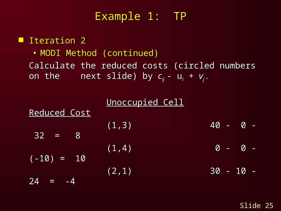
Slide 25 of 82 Slide 25 of 82
Example 1: TPExample 1: TP
Iteration 2Iteration 2• MODI Method (continued)MODI Method (continued)
Calculate the reduced costs (circled Calculate the reduced costs (circled numbers on the numbers on the next slide) by next slide) by ccijij - u- uii + + vvjj..
Unoccupied CellUnoccupied Cell Reduced CostReduced Cost
(1,3) (1,3) 40 - 0 - 32 = 840 - 0 - 32 = 8
(1,4) (1,4) 0 - 0 - (-10) 0 - 0 - (-10) = 10= 10
(2,1) (2,1) 30 - 10 - 24 = -430 - 10 - 24 = -4

Slide 26 of 82 Slide 26 of 82
Example 1: TPExample 1: TP
Iteration 2 TableauIteration 2 Tableau
2525 2525 25 25 25 25
-4 -4 -4 -4
+8 +8 +8 +8 +10 +10 +10 +10
20 20 20 20 10 10 10 10 20 20 20 20 42424242
40404040 0000
000040404040
30303030
30303030
vvjj
uuii
1010
00
-6-6363630302424
DummyDummy
Plant 1Plant 1
Plant 2Plant 2
EastwoodEastwoodWestwoodWestwoodNorthwoodNorthwood
24242424

Slide 27 of 82 Slide 27 of 82
Example 1: TPExample 1: TP
Iteration 2Iteration 2• Stepping Stone MethodStepping Stone Method
The most negative reduced cost is = -4 The most negative reduced cost is = -4 determined by determined by xx2121. The stepping stone path for this . The stepping stone path for this cell is (2,1),(1,1),(1,2),(2,2). The allocations in the cell is (2,1),(1,1),(1,2),(2,2). The allocations in the subtraction cells are 25 and 20 respectively. Thus subtraction cells are 25 and 20 respectively. Thus the new solution is obtained by reallocating 20 on the new solution is obtained by reallocating 20 on the stepping stone path. Thus for the next tableau:the stepping stone path. Thus for the next tableau:
xx2121 = 0 + 20 = 20 (0 is its current allocation) = 0 + 20 = 20 (0 is its current allocation)
xx1111 = 25 - 20 = 5 = 25 - 20 = 5
xx1212 = 25 + 20 = 45 = 25 + 20 = 45
xx2222 = 20 - 20 = 0 (blank for the next tableau) = 20 - 20 = 0 (blank for the next tableau) The other occupied cells remain the same.The other occupied cells remain the same.

Slide 28 of 82 Slide 28 of 82
Example 1: TPExample 1: TP
Iteration 3Iteration 3• MODI MethodMODI Method
The reduced costs are found by calculating The reduced costs are found by calculating the the uuii's and 's and vvjj's for this tableau.'s for this tableau.
1. Set 1. Set uu11 = 0 = 0
2. Since 2. Since uu11 + + vvjj = = cc11jj for occupied cells in row 1, for occupied cells in row 1, thenthen
vv11 = 24 and = 24 and vv22 = 30. = 30.
3. Since 3. Since uuii + + vv11 = = ccii11 for occupied cells in column 2, for occupied cells in column 2, then then uu22 + 24 = 30 or + 24 = 30 or uu22 = 6. = 6.
4. Since 4. Since uu22 + + vvjj = = cc22jj for occupied cells in row 2, for occupied cells in row 2, thenthen
6 + 6 + vv33 = 42 or = 42 or vv33 = 36, and 6 + = 36, and 6 + vv44 = 0 or = 0 or vv44 = -6. = -6.

Slide 29 of 82 Slide 29 of 82
Example 1: TPExample 1: TP
Iteration 3Iteration 3• MODI Method (continued)MODI Method (continued)
Calculate the reduced costs (circled Calculate the reduced costs (circled numbers on the numbers on the next slide) by next slide) by ccijij - - uuii + + vvjj..
Unoccupied CellUnoccupied Cell Reduced CostReduced Cost
(1,3) (1,3) 40 - 0 - 36 = 4 40 - 0 - 36 = 4
(1,4) (1,4) 0 - 0 - (-6) 0 - 0 - (-6) = 6= 6
(2,2) (2,2) 40 - 6 - 30 = 4 40 - 6 - 30 = 4

Slide 30 of 82 Slide 30 of 82
Example 1: TPExample 1: TP
Iteration 3 TableauIteration 3 Tableau
Since all the reduced costs are non-Since all the reduced costs are non-negative, this is the optimal tableau.negative, this is the optimal tableau.
55 55 45 45 45 45
20 20 20 20
+4 +4 +4 +4 +6 +6 +6 +6
+4 +4 +4 +4 10 10 10 10 20 20 20 20 42424242
40404040 0000
000040404040
30303030
30303030
vvjj
uuii
66
00
-6-6363630302424
DummyDummy
Plant 1Plant 1
Plant 2Plant 2
EastwoodEastwoodWestwoodWestwoodNorthwoodNorthwood
24242424

Slide 31 of 82 Slide 31 of 82
Example 1: TPExample 1: TP
Optimal SolutionOptimal Solution
FromFrom ToTo AmountAmount CostCost
Plant 1 Northwood 5 120Plant 1 Northwood 5 120
Plant 1 Westwood 45 1,350Plant 1 Westwood 45 1,350
Plant 2 Northwood 20 600Plant 2 Northwood 20 600
Plant 2 Eastwood 10 Plant 2 Eastwood 10 420420
Total Cost = $2,490Total Cost = $2,490

Slide 32 of 82 Slide 32 of 82
Example 2: TPExample 2: TP
Des MoinesDes Moines(100 units (100 units capacity)capacity)
ClevelandCleveland(200 units(200 unitsReq.)Req.)
Boston (200Boston (200units req.)units req.)
Fort LauderdaleFort Lauderdale(300 units capacity)(300 units capacity)
Albuquerque Albuquerque (300 units(300 unitsReq.)Req.) Evansville (300Evansville (300
units capacity)units capacity)

Slide 33 of 82 Slide 33 of 82
Example 2: TPExample 2: TP
To (Destination)
From(Sources)
Albuquerque Boston Cleveland
Des Moines $5 $4 $3
Evansville $8 $4 $3
FortLauderdale
$9 $7 $5

Slide 34 of 82 Slide 34 of 82
To Factory
From Albu-querque
Boston Cleve-land
capacity
Des 5 4 3 100MoinesEvansville 8 4 3 300
Fort 9 7 5 300LauderdaleWarehouserequirement
300 200 200 700
Example 2: TPExample 2: TP

Slide 35 of 82 Slide 35 of 82
Example 2: TPExample 2: TP
What is the initial solution?What is the initial solution?• Since we want to minimize the cost, it is Since we want to minimize the cost, it is
reasonable to “be greedy” and start at the reasonable to “be greedy” and start at the cheapest cell ($3/unit) while shipping as much cheapest cell ($3/unit) while shipping as much as possible. This method of getting the initial as possible. This method of getting the initial feasible solution is called the least-cost rulefeasible solution is called the least-cost rule
• Any ties are broken arbitrarily. Any ties are broken arbitrarily. (Des Moines to Cleveland - $3)(Des Moines to Cleveland - $3)(Evansville to Cleveland - $3)(Evansville to Cleveland - $3)Let’s start ad cell 1-3 (Des Moines to Cleveland)Let’s start ad cell 1-3 (Des Moines to Cleveland)
• In making the flow assignments make sure not In making the flow assignments make sure not to exceed the capacities and demands on the to exceed the capacities and demands on the margins!margins!

Slide 36 of 82 Slide 36 of 82
To Factory
From Albu-querque
Boston Cleve-land
capacity
Des 5 4 3 100MoinesEvansville 8 4 3 300
Fort 9 7 5 300LauderdaleWarehouserequirement
300 200 200 700
Example 2: TPExample 2: TP
StartStart +100+100 00
100100

Slide 37 of 82 Slide 37 of 82
To Factory
From Albu-querque
Boston Cleve-land
capacity
Des 5 4 3 100MoinesEvansville 8 4 3 300
Fort 9 7 5 300LauderdaleWarehouserequirement
300 200 200 700
Example 2: TPExample 2: TP
+100+100
+100+100
00
100100
200200
00

Slide 38 of 82 Slide 38 of 82
To Factory
From Albu-querque
Boston Cleve-land
capacity
Des 5 4 3 100MoinesEvansville 8 4 3 300
Fort 9 7 5 300LauderdaleWarehouserequirement
300 200 200 700
Example 2: TPExample 2: TP
+100+100
+200 +100+200 +100
00
100100
200200
0000
00

Slide 39 of 82 Slide 39 of 82
To Factory
From Albu-querque
Boston Cleve-land
capacity
Des 5 4 3 100MoinesEvansville 8 4 3 300
Fort 9 7 5 300LauderdaleWarehouserequirement
300 200 200 700
Example 2: TPExample 2: TP
+100+100
+200 +100+200 +100
+300+300
00
100100
200200
0000
00
00
00

Slide 40 of 82 Slide 40 of 82
Example 2: TPExample 2: TP
The initial feasible solution via the least-cost rule The initial feasible solution via the least-cost rule is:is:• Ship 100 units from Des Moines to ClevelandShip 100 units from Des Moines to Cleveland• Ship 100 units from Evansville to ClevelandShip 100 units from Evansville to Cleveland• Ship 200 units from Evansville to BostonShip 200 units from Evansville to Boston• Ship 300 units from Fort Lauderdale to Ship 300 units from Fort Lauderdale to
AlbuquerqueAlbuquerque The total cost of this solution is:The total cost of this solution is:
• 100(3) + 100(3) + 200(4) + 300(9) = $4,100100(3) + 100(3) + 200(4) + 300(9) = $4,100 Is the current solution optimal?Is the current solution optimal?
• Perhaps, but we are not sure. Hence, some Perhaps, but we are not sure. Hence, some more work is needed.more work is needed.

Slide 41 of 82 Slide 41 of 82
Example 2: TPExample 2: TP
The cells that have a number in them are The cells that have a number in them are referred to as basic cells (or referred to as basic cells (or basic variablesbasic variables))• In general, all basic variables are strictly In general, all basic variables are strictly
positivepositive• When at least one basic variable is equal to When at least one basic variable is equal to
zero, the corresponding solution is called zero, the corresponding solution is called degeneratedegenerate
• When a solution is degenerate, exercise When a solution is degenerate, exercise caution in using sensitivity reportscaution in using sensitivity reports

Slide 42 of 82 Slide 42 of 82
Example 2: TPExample 2: TP
How many basic variables (cells) should there be How many basic variables (cells) should there be in the transportation tableau?in the transportation tableau?• Answer: (R+C-1), where R = number of rows Answer: (R+C-1), where R = number of rows
and C = number of columns. Here, (R+C-1) = and C = number of columns. Here, (R+C-1) = 3+3-1 = 53+3-1 = 5
What are they (there are 4 of them)?What are they (there are 4 of them)?• Ship 100 units from Des Moines to ClevelandShip 100 units from Des Moines to Cleveland• Ship 100 units from Evansville to ClevelandShip 100 units from Evansville to Cleveland• Ship 200 units from Evansville to BostonShip 200 units from Evansville to Boston• Ship 300 units from Fort Lauderdale to Ship 300 units from Fort Lauderdale to
AlbuquerqueAlbuquerque

Slide 43 of 82 Slide 43 of 82
Example 2: TPExample 2: TP
Is this solution degenerate?Is this solution degenerate?• Answer: Yes, because (R+C-1) = 3+3-1 = 5 > Answer: Yes, because (R+C-1) = 3+3-1 = 5 >
44• Hence, we can arbitrarily make (5-4) = 1 Hence, we can arbitrarily make (5-4) = 1
variable which is at level zero basic. variable which is at level zero basic. • Let us make Des Moines to Albuquerque a Let us make Des Moines to Albuquerque a
basic variable at level zerobasic variable at level zero How do we determine if the current solution is How do we determine if the current solution is
optimal?optimal?• Let us price currently nonbasic variables Let us price currently nonbasic variables
(cells), which are all at level zero using the (cells), which are all at level zero using the stepping stonestepping stone algorithm algorithm

Slide 44 of 82 Slide 44 of 82
To Factory
From Albu-querque
Boston Cleve-land
capacity
Des 5 4 3 100MoinesEvansville 8 4 3 300
Fort 9 7 5 300LauderdaleWarehouserequirement
300 200 200 700
Example 2: TPExample 2: TP
0 0 +100 +100
+200 +100 +200 +100
+300+300

Slide 45 of 82 Slide 45 of 82
Example 2: TPExample 2: TP
Evansville – Albuquerque:Evansville – Albuquerque:• 8 – 3 + 3 – 5 = 3 > 08 – 3 + 3 – 5 = 3 > 0

Slide 46 of 82 Slide 46 of 82
To Factory
From Albu-querque
Boston Cleve-land
capacity
Des 5 4 3 100MoinesEvansville 8 4 3 300
Fort 9 7 5 300LauderdaleWarehouserequirement
300 200 200 700
Example 2: TPExample 2: TP
0 0 +100 +100
+200 +100 +200 +100
+300+300

Slide 47 of 82 Slide 47 of 82
Example 2: TPExample 2: TP
Des Moines - Boston:Des Moines - Boston:• 4 – 3 + 3 - 4 = 04 – 3 + 3 - 4 = 0

Slide 48 of 82 Slide 48 of 82
To Factory
From Albu-querque
Boston Cleve-land
capacity
Des 5 4 3 100MoinesEvansville 8 4 3 300
Fort 9 7 5 300LauderdaleWarehouserequirement
300 200 200 700
Example 2: TPExample 2: TP
0 0 +100 +100
+200 +100 +200 +100
+300+300

Slide 49 of 82 Slide 49 of 82
Example 2: TPExample 2: TP
Fort Lauderdale - Boston:Fort Lauderdale - Boston:• 7 – 9 + 5 - 3 + 3 – 4 = -1 < 07 – 9 + 5 - 3 + 3 – 4 = -1 < 0

Slide 50 of 82 Slide 50 of 82
To Factory
From Albu-querque
Boston Cleve-land
capacity
Des 5 4 3 100MoinesEvansville 8 4 3 300
Fort 9 7 5 300LauderdaleWarehouserequirement
300 200 200 700
Example 2: TPExample 2: TP
0 0 +100 +100
+200 +100 +200 +100
+300+300

Slide 51 of 82 Slide 51 of 82
Example 2: TPExample 2: TP
Fort Lauderdale - Cleveland:Fort Lauderdale - Cleveland:• 5 –29 + 5 - 3 = -2 < 05 –29 + 5 - 3 = -2 < 0

Slide 52 of 82 Slide 52 of 82
Example 1: TPExample 1: TP
The objective function improvement potentials The objective function improvement potentials for the nonbasic variables are:for the nonbasic variables are:• Evansville – Albuquerque: 3 > 0Evansville – Albuquerque: 3 > 0• Des Moines - Boston: 0 = 0Des Moines - Boston: 0 = 0• Fort Lauderdale - Boston: -1 < 0Fort Lauderdale - Boston: -1 < 0• Fort Lauderdale - Cleveland: Fort Lauderdale - Cleveland: -2 < 0-2 < 0
The largest improvement (here: reduction in The largest improvement (here: reduction in cost) in the objective function can be achieved cost) in the objective function can be achieved by increasing shipments from Fort Lauderdale to by increasing shipments from Fort Lauderdale to ClevelandCleveland
What i2 the limit on the increase?What i2 the limit on the increase?

Slide 53 of 82 Slide 53 of 82
To Factory
From Albu-querque
Boston Cleve-land
capacity
Des 5 4 3 100MoinesEvansville 8 4 3 300
Fort 9 7 5 300LauderdaleWarehouserequirement
300 200 200 700
Example 2 TPExample 2 TP
0 0 +K+K +100 +100 -K-K
+200 +100 +200 +100
+300 +300 -K-K +K+K

Slide 54 of 82 Slide 54 of 82
Example 2: TPExample 2: TP
If we increase shipments from Fort Lauderdale to If we increase shipments from Fort Lauderdale to Cleveland by K, we must reduce shipments in Cleveland by K, we must reduce shipments in the basic cells in the same row and column so the basic cells in the same row and column so that the totals on the margins remain the samethat the totals on the margins remain the same
Clearly, because negative quantities cannot be Clearly, because negative quantities cannot be shipped, we must impose that:shipped, we must impose that:• K >= 0 (no problem)K >= 0 (no problem)• 300 – K >= 0 (K <= 300)300 – K >= 0 (K <= 300)• 0 + K >= 0 (no problem)0 + K >= 0 (no problem)• 100 – K >=0 (K <=100)100 – K >=0 (K <=100)
Hence, let K = 100Hence, let K = 100 The new basis becomes:The new basis becomes:
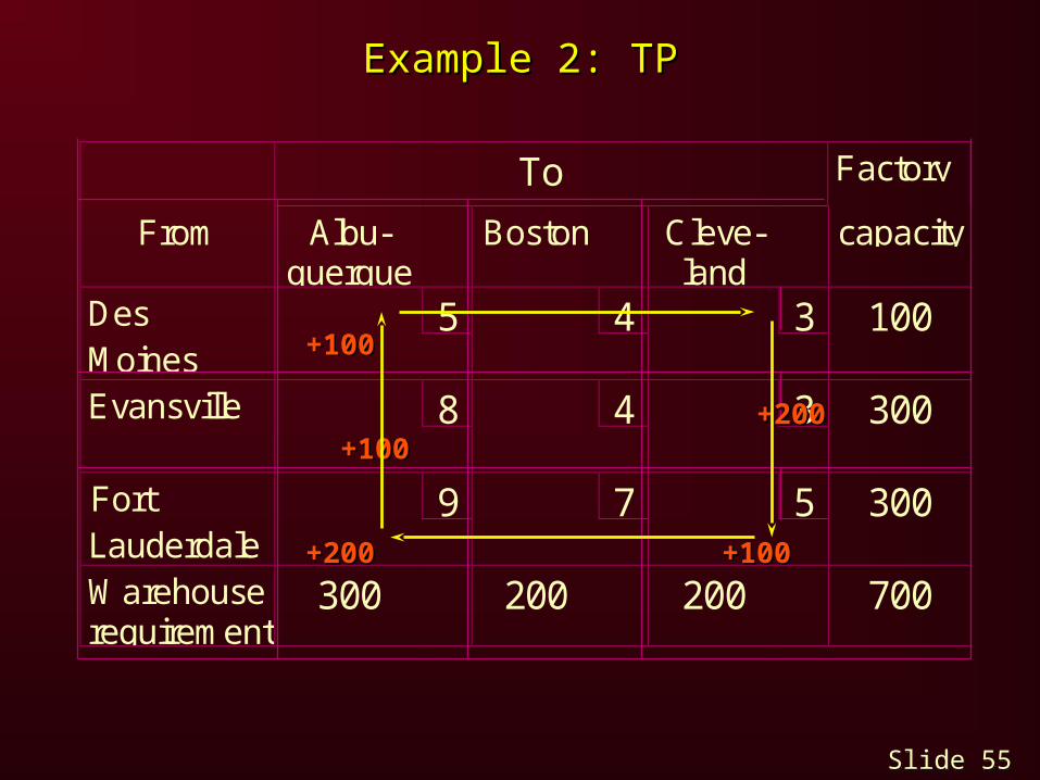
Slide 55 of 82 Slide 55 of 82
To Factory
From Albu-querque
Boston Cleve-land
capacity
Des 5 4 3 100MoinesEvansville 8 4 3 300
Fort 9 7 5 300LauderdaleWarehouserequirement
300 200 200 700
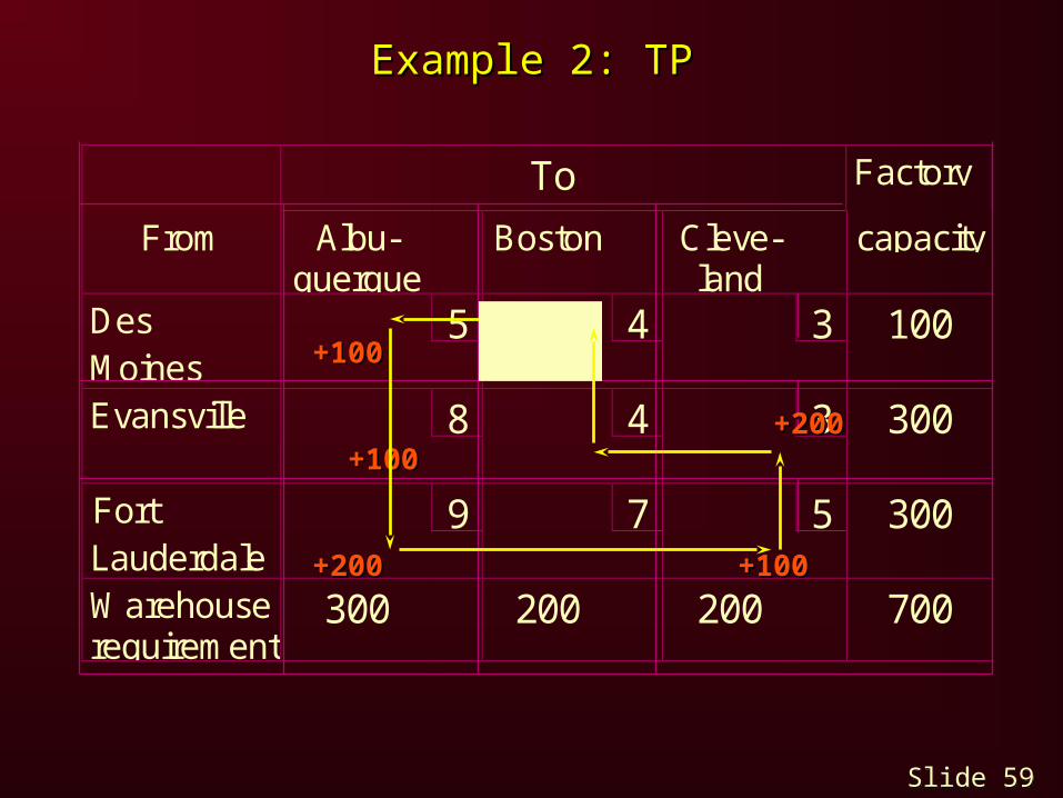
Example 2: TPExample 2: TP
+100+100
+200 +100 +200 +100
+200+200 +100 +100

Slide 56 of 82 Slide 56 of 82
Example 2: TPExample 2: TP
Observe that the number of basic variables Observe that the number of basic variables (cells) is equal to (R+C-1) = 5. Hence, the (cells) is equal to (R+C-1) = 5. Hence, the current basic solution is feasible and not current basic solution is feasible and not degeneratedegenerate
Also observe that Des Moines – Cleveland left the Also observe that Des Moines – Cleveland left the basis while Fort Lauderdale – Cleveland entered basis while Fort Lauderdale – Cleveland entered the basis (one for one interchange)the basis (one for one interchange)
Is the current solution optimal?Is the current solution optimal?• Let us price the non-basic variables (cells):Let us price the non-basic variables (cells):

Slide 57 of 82 Slide 57 of 82
To Factory
From Albu-querque
Boston Cleve-land
capacity
Des 5 4 3 100MoinesEvansville 8 4 3 300
Fort 9 7 5 300LauderdaleWarehouserequirement
300 200 200 700
Example 2: TPExample 2: TP
+100+100
+200 +100 +200 +100
+200+200 +100 +100
Slide 58 of 82 Slide 58 of 82
Example 2: TPExample 2: TP
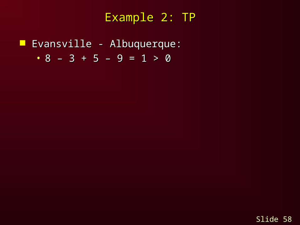
Evansville - Albuquerque:Evansville - Albuquerque:• 8 – 3 + 5 – 9 = 1 > 08 – 3 + 5 – 9 = 1 > 0
Slide 59 of 82 Slide 59 of 82
To Factory
From Albu-querque
Boston Cleve-land
capacity
Des 5 4 3 100MoinesEvansville 8 4 3 300
Fort 9 7 5 300LauderdaleWarehouserequirement
300 200 200 700
Example 2: TPExample 2: TP
+100+100
+200 +100 +200 +100
+200+200 +100 +100

Slide 60 of 82 Slide 60 of 82
Example 2: TPExample 2: TP
Des Moines - Boston:Des Moines - Boston:• 4 – 5 + 9 – 5 + 3 – 4 = 2 > 04 – 5 + 9 – 5 + 3 – 4 = 2 > 0

Slide 61 of 82 Slide 61 of 82
To Factory
From Albu-querque
Boston Cleve-land
capacity
Des 5 4 3 100MoinesEvansville 8 4 3 300
Fort 9 7 5 300LauderdaleWarehouserequirement
300 200 200 700
Example 2: TPExample 2: TP
+100+100
+200 +100 +200 +100
+200+200 +100 +100

Slide 62 of 82 Slide 62 of 82
Example 2: TPExample 2: TP
Fort Lauderdale - Boston:Fort Lauderdale - Boston:• 7 – 5 + 3 - 4 = 1 > 07 – 5 + 3 - 4 = 1 > 0

Slide 63 of 82 Slide 63 of 82
To Factory
From Albu-querque
Boston Cleve-land
capacity
Des 5 4 3 100MoinesEvansville 8 4 3 300
Fort 9 7 5 300LauderdaleWarehouserequirement
300 200 200 700
Example 2: TPExample 2: TP
+100+100
+200 +100 +200 +100
+200+200 +100 +100

Slide 64 of 82 Slide 64 of 82
Example 2: TPExample 2: TP
Des Moines - Cleveland:Des Moines - Cleveland:• 3 – 5 + 9 - 5 = 2 > 03 – 5 + 9 - 5 = 2 > 0

Slide 65 of 82 Slide 65 of 82
Example 2: TPExample 2: TP
The objective function improvement potentials The objective function improvement potentials for the nonbasic variables are:for the nonbasic variables are:• Evansville - Albuquerque: 1 > 0Evansville - Albuquerque: 1 > 0• Des Moines - Boston: 2 > 0Des Moines - Boston: 2 > 0• Fort Lauderdale - Boston: 1 > 0Fort Lauderdale - Boston: 1 > 0• Des Moines - Cleveland: 2 > 0Des Moines - Cleveland: 2 > 0
Since all improvement potentials are positive, it Since all improvement potentials are positive, it is not possible to achieve further improvement is not possible to achieve further improvement (here: reduction in cost) in the objective function (here: reduction in cost) in the objective function
Hence, the current solution is optimalHence, the current solution is optimal
Slide 66 of 82 Slide 66 of 82
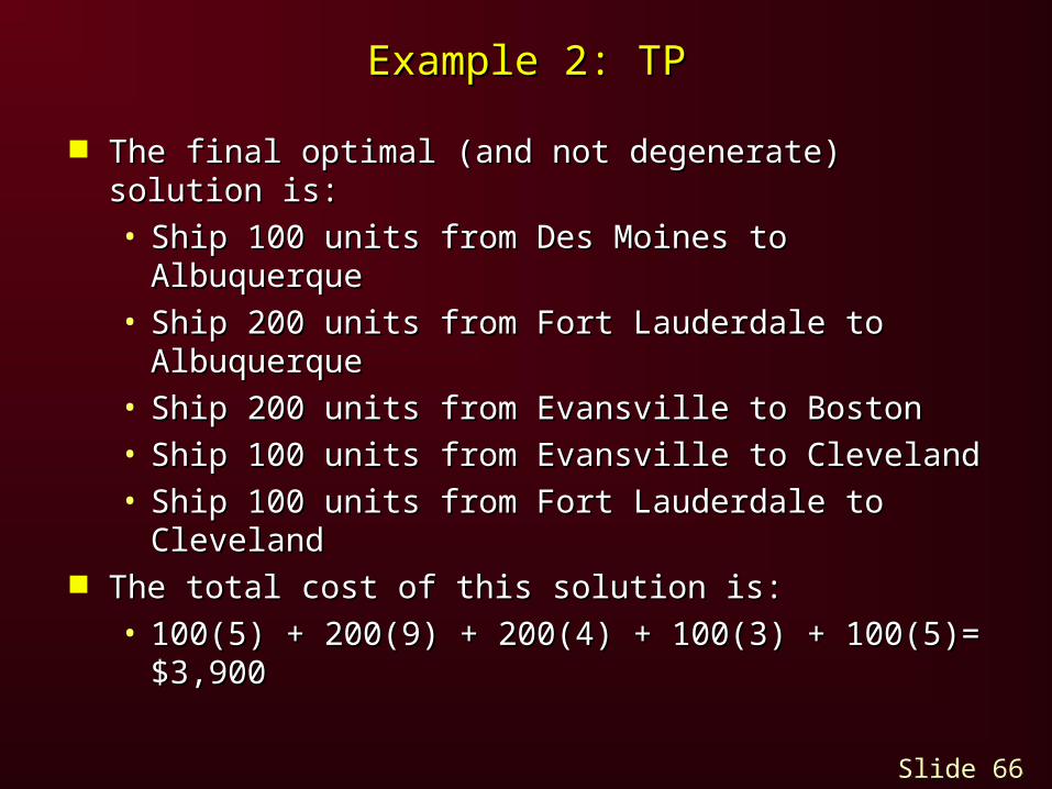
Example 2: TPExample 2: TP
The final optimal (and not degenerate) solution is:The final optimal (and not degenerate) solution is:• Ship 100 units from Des Moines to AlbuquerqueShip 100 units from Des Moines to Albuquerque• Ship 200 units from Fort Lauderdale to Ship 200 units from Fort Lauderdale to
AlbuquerqueAlbuquerque• Ship 200 units from Evansville to BostonShip 200 units from Evansville to Boston• Ship 100 units from Evansville to Cleveland Ship 100 units from Evansville to Cleveland • Ship 100 units from Fort Lauderdale to Ship 100 units from Fort Lauderdale to
ClevelandCleveland The total cost of this solution is:The total cost of this solution is:
• 100(5) + 200(9) + 200(4) + 100(3) + 100(5)= 100(5) + 200(9) + 200(4) + 100(3) + 100(5)= $3,900$3,900
Slide 67 of 82 Slide 67 of 82
Example 2: TP via LPExample 2: TP via LP
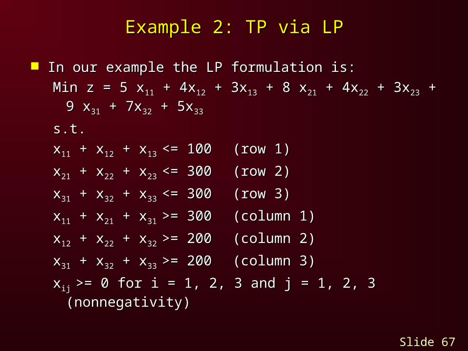
In our example the LP formulation is:In our example the LP formulation is:
Min z = 5 xMin z = 5 x1111 + 4x + 4x1212 + 3x + 3x1313 + 8 x + 8 x2121 + 4x + 4x2222 + 3x + 3x2323 + 9 + 9 xx3131 + 7x + 7x3232 + 5x + 5x3333
s.t.s.t.
xx1111 + x + x1212 + x + x13 13 <= 100<= 100 (row 1)(row 1)
xx2121 + x + x2222 + x + x23 23 <= 300<= 300 (row 2)(row 2)
xx3131 + x + x3232 + x + x33 33 <= 300<= 300 (row 3)(row 3)
xx1111 + x + x2121 + x + x31 31 >= 300>= 300 (column 1)(column 1)
xx1212 + x + x2222 + x + x32 32 >= 200>= 200 (column 2)(column 2)
xx3131 + x + x3232 + x + x33 33 >= 200>= 200 (column 3)(column 3)
xxij ij >= 0 for i = 1, 2, 3 and j = 1, 2, 3 (nonnegativity)>= 0 for i = 1, 2, 3 and j = 1, 2, 3 (nonnegativity)
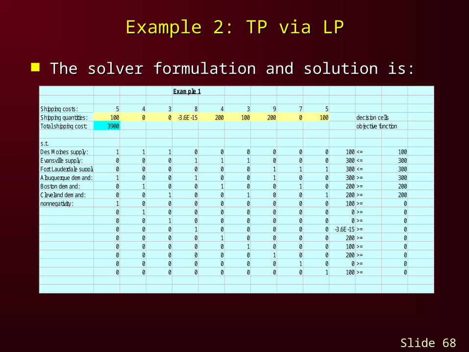
Slide 68 of 82 Slide 68 of 82
Example 2: TP via LPExample 2: TP via LP
The solver formulation and solution is:The solver formulation and solution is:Example 1
Shipping costs: 5 4 3 8 4 3 9 7 5Shipping quantities: 100 0 0 -3.6E-15 200 100 200 0 100 decision cellsTotal shipping cost: 3900 objective function
s.t.Des Moines supply: 1 1 1 0 0 0 0 0 0 100 <= 100Evansville supply: 0 0 0 1 1 1 0 0 0 300 <= 300Fort Lauderdale supply: 0 0 0 0 0 0 1 1 1 300 <= 300Albuquerque demand: 1 0 0 1 0 0 1 0 0 300 >= 300Boston demand: 0 1 0 0 1 0 0 1 0 200 >= 200Cleveland demand: 0 0 1 0 0 1 0 0 1 200 >= 200nonnegativity: 1 0 0 0 0 0 0 0 0 100 >= 0
0 1 0 0 0 0 0 0 0 0 >= 00 0 1 0 0 0 0 0 0 0 >= 00 0 0 1 0 0 0 0 0 -3.6E-15 >= 00 0 0 0 1 0 0 0 0 200 >= 00 0 0 0 0 1 0 0 0 100 >= 00 0 0 0 0 0 1 0 0 200 >= 00 0 0 0 0 0 0 1 0 0 >= 00 0 0 0 0 0 0 0 1 100 >= 0

Slide 69 of 82 Slide 69 of 82
Example 2: TP via LPExample 2: TP via LP
The solver answer report is:The solver answer report is:Microsoft Excel 9.0 Answer ReportWorksheet: [Example 1 - TP via LP.xls]Sheet1Report Created: 2/9/00 12:12:55 PM
Target Cell (Min)Cell Name Original Value Final Value
$B$5 WBMIN 3900 3900
Adjustable CellsCell Name Original Value Final Value
$B$4 Shipping quantities: 100 100$C$4 Shipping quantities: 0 0$D$4 Shipping quantities: 0 0$E$4 Shipping quantities: Example 1 -3.55271E-15 -3.55271E-15$F$4 Shipping quantities: 200 200$G$4 Shipping quantities: 100 100$H$4 Shipping quantities: 200 200$I$4 Shipping quantities: 0 0$J$4 Shipping quantities: 100 100
ConstraintsCell Name Cell Value Formula Status Slack
$K$10 Fort Lauderdale supply: 300 $K$10<=$M$10 Binding 0$K$8 Des Moines supply: 100 $K$8<=$M$8 Binding 0$K$12 Boston demand: 200 $K$12>=$M$12 Binding 0$K$9 Evansville supply: 300 $K$9<=$M$9 Binding 0$K$11 Albuquerque demand: 300 $K$11>=$M$11 Binding 0$K$13 Cleveland demand: 200 $K$13>=$M$13 Binding 0$K$14 nonnegativity: 100 $K$14>=$M$14 Not Binding 100$K$15 0 $K$15>=$M$15 Binding 0$K$16 0 $K$16>=$M$16 Binding 0$K$17 -3.55271E-15 $K$17>=$M$17 Binding 0$K$18 200 $K$18>=$M$18 Not Binding 200$K$20 200 $K$20>=$M$20 Not Binding 200$K$21 0 $K$21>=$M$21 Binding 0$K$22 100 $K$22>=$M$22 Not Binding 100$K$19 100 $K$19>=$M$19 Not Binding 100

Slide 70 of 82 Slide 70 of 82
Example 2: TP via LPExample 2: TP via LP
The solver sensitivity report is:The solver sensitivity report is:Microsoft Excel 9.0 Sensitivity ReportWorksheet: [Example 1 - TP via LP.xls]Sheet1Report Created: 2/9/00 12:12:55 PM
Adjustable CellsFinal Reduced
Cell Name Value Gradient$B$4 Shipping quantities: 100 0$C$4 Shipping quantities: 0 0$D$4 Shipping quantities: 0 0$E$4 Shipping quantities: Example 1 -3.55271E-15 0$F$4 Shipping quantities: 200 0$G$4 Shipping quantities: 100 0$H$4 Shipping quantities: 200 0$I$4 Shipping quantities: 0 0$J$4 Shipping quantities: 100 0
ConstraintsFinal Lagrange
Cell Name Value Multiplier$K$10 Fort Lauderdale supply: 300 0$K$8 Des Moines supply: 100 -4$K$12 Boston demand: 200 6$K$9 Evansville supply: 300 -2$K$11 Albuquerque demand: 300 9$K$13 Cleveland demand: 200 5$K$14 nonnegativity: 100 0$K$15 0 1.999998689$K$16 0 2.00000006$K$17 -3.55271E-15 0.999999642$K$18 200 0$K$20 200 0$K$21 0 0.999998927$K$22 100 0$K$19 100 0

Slide 71 of 82 Slide 71 of 82
Example 2: TP via LPExample 2: TP via LP
The solver limits report is:The solver limits report is:Microsoft Excel 9.0 Limits ReportWorksheet: [Example 1 - TP via LP.xls]Sheet1Report Created: 2/9/00 12:12:55 PM
TargetCell Name Value
$B$5 WBMIN 3900
Adjustable Lower Target Upper TargetCell Name Value Limit Result Limit Result
$B$4 Shipping quantities: 100 100 3900 100 3900$C$4 Shipping quantities: 0 0 3900 0 3900$D$4 Shipping quantities: 0 0 3900 0 3900$E$4 Shipping quantities: Example 1 -3.55271E-15 -3.55271E-15 3900 -3.55271E-15 3900$F$4 Shipping quantities: 200 200 3900 200 3900$G$4 Shipping quantities: 100 100 3900 100 3900$H$4 Shipping quantities: 200 200 3900 200 3900$I$4 Shipping quantities: 0 0 3900 0 3900$J$4 Shipping quantities: 100 100 3900 100 3900
Slide 72 of 82 Slide 72 of 82
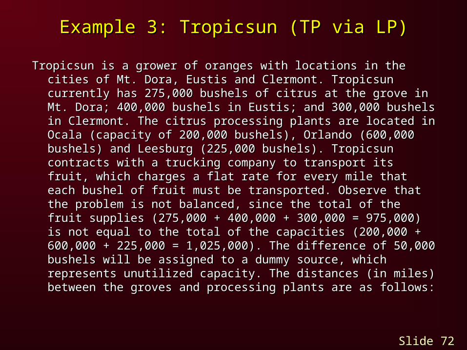
Example 3: Tropicsun (TP via LP)Example 3: Tropicsun (TP via LP)
Tropicsun is a grower of oranges with locations in the cities of Tropicsun is a grower of oranges with locations in the cities of Mt. Dora, Eustis and Clermont. Tropicsun currently has Mt. Dora, Eustis and Clermont. Tropicsun currently has 275,000 bushels of citrus at the grove in Mt. Dora; 400,000 275,000 bushels of citrus at the grove in Mt. Dora; 400,000 bushels in Eustis; and 300,000 bushels in Clermont. The bushels in Eustis; and 300,000 bushels in Clermont. The citrus processing plants are located in Ocala (capacity of citrus processing plants are located in Ocala (capacity of 200,000 bushels), Orlando (600,000 bushels) and Leesburg 200,000 bushels), Orlando (600,000 bushels) and Leesburg (225,000 bushels). Tropicsun contracts with a trucking (225,000 bushels). Tropicsun contracts with a trucking company to transport its fruit, which charges a flat rate for company to transport its fruit, which charges a flat rate for every mile that each bushel of fruit must be transported. every mile that each bushel of fruit must be transported. Observe that the problem is not balanced, since the total of Observe that the problem is not balanced, since the total of the fruit supplies (275,000 + 400,000 + 300,000 = the fruit supplies (275,000 + 400,000 + 300,000 = 975,000) is not equal to the total of the capacities (200,000 975,000) is not equal to the total of the capacities (200,000 + 600,000 + 225,000 = 1,025,000). The difference of + 600,000 + 225,000 = 1,025,000). The difference of 50,000 bushels will be assigned to a dummy source, which 50,000 bushels will be assigned to a dummy source, which represents unutilized capacity. The distances (in miles) represents unutilized capacity. The distances (in miles) between the groves and processing plants are as follows:between the groves and processing plants are as follows:

Slide 73 of 82 Slide 73 of 82
Example 3: Tropicsun (TP via LP)Example 3: Tropicsun (TP via LP)
Distances (in miles) between groves and plantsDistances (in miles) between groves and plantsGroveGrove OcalaOcala OrlandoOrlando LeesburgLeesburg
Mt. DoraMt. Dora 2121 5050 4040
EustisEustis 3535 3030 2222
ClermontClermont 5555 2020 2525

Slide 74 of 82 Slide 74 of 82
Example 3: TP via LPExample 3: TP via LP : :TropicsunTropicsun
Mt. Dora
1
Eustis
2
Clermont
3
Ocala
4
Orlando
5
Leesburg
6
Distances (in miles)CapacitySupply
275,000
400,000
300,000 225,000
600,000
200,000
GrovesProcessing Plants
21
50
40
3530
22
55
25
20

Slide 75 of 82 Slide 75 of 82
Example 3: Defining the Decision VariablesExample 3: Defining the Decision Variables
Xij = # of bushels shipped from node i to node j
Specifically, the nine decision variables are:
X14 = # of bushels shipped from Mt. Dora (node 1) to Ocala (node 4)
X15 = # of bushels shipped from Mt. Dora (node 1) to Orlando (node 5)
X16 = # of bushels shipped from Mt. Dora (node 1) to Leesburg (node 6)
X24 = # of bushels shipped from Eustis (node 2) to Ocala (node 4)
X25 = # of bushels shipped from Eustis (node 2) to Orlando (node 5)
X26 = # of bushels shipped from Eustis (node 2) to Leesburg (node 6)
X34 = # of bushels shipped from Clermont (node 3) to Ocala (node 4)
X35 = # of bushels shipped from Clermont (node 3) to Orlando (node 5)
X36 = # of bushels shipped from Clermont (node 3) to Leesburg (node 6)

Slide 76 of 82 Slide 76 of 82
Example 3: Defining the Objective FunctionExample 3: Defining the Objective Function
Minimize the total number of bushel-miles.
MIN: 21X14 + 50X15 + 40X16 +
35X24 + 30X25 + 22X26 +
55X34 + 20X35 + 25X36

Slide 77 of 82 Slide 77 of 82
Example 3: Defining the ConstraintsExample 3: Defining the Constraints
Capacity constraintsCapacity constraints
XX1414 + X + X2424 + X + X3434 <= 200,000 <= 200,000 } Ocala} Ocala
XX1515 + X + X2525 + X + X3535 <= 600,000 <= 600,000 } Orlando} Orlando
XX1616 + X + X2626 + X + X3636 <= 225,000 <= 225,000 } Leesburg} Leesburg
Supply constraintsSupply constraints
XX1414 + X + X1515 + X + X1616 = 275,000 = 275,000 } Mt. Dora} Mt. Dora
XX2424 + X + X2525 + X + X2626 = 400,000 = 400,000 } Eustis} Eustis
XX3434 + X + X3535 + X + X3636 = 300,000 = 300,000 } Clermont} Clermont
Nonnegativity conditionsNonnegativity conditionsXXijij >= 0 for all >= 0 for all i i andand j j

Slide 78 of 82 Slide 78 of 82
Example 3: Solver FormulationExample 3: Solver Formulation
Distances FromGroves to Plant at:
Grove Ocala Orlando LeesburgMt. Dora 21 50 40Eustis 35 30 22Clermont 55 20 25
Bushels Shipped FromGroves to Plant at: Bushels Bushels
Grove Ocala Orlando Leesburg Shipped AvailableMt. Dora 0 0 0 0 275,000Eustis 0 0 0 0 400,000Clermont 0 0 0 0 300,000Received 0 0 0Capacity 200,000 600,000 225,000
Total Distance (in bushel-miles): 0
Tropicsun

Slide 79 of 82 Slide 79 of 82
Example 3: Solver SolutionExample 3: Solver Solution
Distances FromGroves to Plant at:
Grove Ocala Orlando LeesburgMt. Dora 21 50 40Eustis 35 30 22Clermont 55 20 25
Bushels Shipped FromGroves to Plant at: Bushels Bushels
Grove Ocala Orlando Leesburg Shipped AvailableMt. Dora 200,000 0 75,000 275,000 275,000Eustis 0 250,000 150,000 400,000 400,000Clermont 0 300,000 0 300,000 300,000Received 200,000 550,000 225,000Capacity 200,000 600,000 225,000
Total Distance (in bushel-miles): 24,000,000
Tropicsun

Slide 80 of 82 Slide 80 of 82
Example 4: The Sentry Lock CorporationExample 4: The Sentry Lock Corporation

Slide 81 of 82 Slide 81 of 82
Example 4: Solver FormulationExample 4: Solver Formulation
Unit Shipping Costs to UnitDistribution Center in: Production
Plants Tacoma San Diego Dallas Denver St. Louis Tampa Baltimore CostMacon $2.50 $2.75 $1.75 $2.00 $2.10 $1.80 $1.65 $35.50Louisville $1.85 $1.90 $1.50 $1.60 $1.00 $1.90 $1.85 $37.50Detroit $2.30 $2.25 $1.85 $1.25 $1.50 $2.25 $2.00 $39.00Phoenix $1.90 $0.90 $1.60 $1.75 $2.00 $2.50 $2.65 $36.25
Quantity Shipped toDistribution Center in: Total
Plants Tacoma San Diego Dallas Denver St. Louis Tampa Baltimore Produced CapacityMacon 0 0 0 0 0 12000 6000 18000 18000Louisville 600 0 0 0 14400 0 0 15000 15000Detroit 400 0 10800 12600 0 0 1200 25000 25000Phoenix 5800 14200 0 0 0 0 0 20000 20000Total Shipped 6800 14200 10800 12600 14400 12000 7200Demand 8500 14500 13500 12600 18000 15000 9000Min Shipped 6800 11600 10800 10080 14400 12000 7200
Total Cost $3,011,360
Sentry Lock Corp.
Minimize: B23By chaning: B15:H18Subject to: I15:I18=J15:J18 B19:H19<=B20:H20 B19:H19>=B21:H21 B15:H18>=0

Slide 82 of 82 Slide 82 of 82
The End of Chapter 2BThe End of Chapter 2B