skp engineering college · 2018-08-28 · s.k.p. engineering college, tiruvannamalai vii sem...
TRANSCRIPT

S.K.P. Engineering College, Tiruvannamalai VII SEM
Electronics and Communication Engineering Department 1 Digital Image Processing
SKP Engineering College
Tiruvannamalai – 606611
A Course Material
on Digital Image Processing
By
S.Nagarajan
Assistant Professor
Electronics and Communication Engineering Department

S.K.P. Engineering College, Tiruvannamalai VII SEM
Electronics and Communication Engineering Department 2 Digital Image Processing
Quality Certificate
This is to Certify that the Electronic Study Material
Subject Code:IT6005
Subject Name:Digital Image Processing
Year/Sem:IV/VII
Being prepared by me and it meets the knowledge requirement of the University curriculum.
Signature of the Author
Name: S.Nagarajan
Designation: Assistant Professor
This is to certify that the course material being prepared by Mr.S.Nagarajan is of the adequate quality. He has referred more than five books and one among them is from abroad author.
Signature of HD Signature of the Principal
Name: Name: Dr.V.Subramania Bharathi
Seal: Seal:

S.K.P. Engineering College, Tiruvannamalai VII SEM
Electronics and Communication Engineering Department 3 Digital Image Processing
IT6005 DIGITAL IMAGE PROCESSING L T P C 3 0 0 3
OBJECTIVES:
The student should be made to: -- Learn digital image fundamentals.
-- Be exposed to simple image processing techniques. -- Be familiar with image compression and segmentation techniques. -- Learn to represent image in form of features.
UNIT I DIGITAL IMAGE FUNDAMENTALS 8 Introduction – Origin – Steps in Digital Image Processing – Components – Elements of Visual Perception – Image Sensing and Acquisition – Image Sampling and Quantization – Relationships between pixels - color models.
UNIT II IMAGE ENHANCEMENT 10
Spatial Domain: Gray level transformations – Histogram processing – Basics of Spatial Filtering–Smoothing and Sharpening Spatial Filtering – Frequency Domain: Introduction to Fourier Transform– Smoothing and Sharpening frequency domain filters – Ideal, Butterworth and Gaussian filters. UNIT III IMAGE RESTORATION AND SEGMENTATION 9 Noise models – Mean Filters – Order Statistics – Adaptive filters – Band reject Filters – Band pass Filters – Notch Filters – Optimum Notch Filtering – Inverse Filtering – Wiener filtering Segmentation:Detection of Discontinuities–Edge Linking and Boundary detection – Region based segmentationMorphological processing-erosion and dilation. UNIT IV WAVELETS AND IMAGE COMPRESSION 9 Wavelets – Subband coding - Multiresolution expansions - Compression: Fundamentals – Image Compression models – Error Free Compression – Variable Length Coding – Bit-Plane Coding – Lossless Predictive Coding – Lossy Compression – Lossy Predictive Coding – Compression Standards. UNIT V IMAGE REPRESENTATION AND RECOGNITION 9 Boundary representation – Chain Code – Polygonal approximation, signature, boundary segments –Boundary description – Shape number – Fourier Descriptor, moments- Regional Descriptors –Topological feature, Texture - Patterns and Pattern classes - Recognition based on matching.
TOTAL: 45 PERIODS TEXT BOOK: 1. Rafael C. Gonzales, Richard E. Woods, “Digital Image Processing”, Third Edition, PearsonEducation, 2010.

S.K.P. Engineering College, Tiruvannamalai VII SEM
Electronics and Communication Engineering Department 4 Digital Image Processing
2. Deitel and Deitel and Nieto, “Internet and World Wide Web - How to Program”, Prentice Hall, 5th Edition, 2011. 3. Herbert Schildt, “Java-The Complete Reference”, Eighth Edition, Mc Graw Hill Professional, 2011. REFERENCES: 1. Rafael C. Gonzalez, Richard E. Woods, Steven L. Eddins, “Digital Image Processing Using MATLAB”, Third Edition Tata Mc Graw Hill Pvt. Ltd., 2011. 2. Anil Jain K. “Fundamentals of Digital Image Processing”, PHI Learning Pvt. Ltd. 2011. 3. Willliam K Pratt, “Digital Image Processing”, John Willey, 2002. 4. Malay K. Pakhira, “Digital Image Processing and Pattern Recognition”, First Edition, PHI Learning Pvt. Ltd., 2011. 5. http://eeweb.poly.edu/~onur/lectures/lectures.html. 6. http://www.caen.uiowa.edu/~dip/LECTURE/lecture.html

S.K.P. Engineering College, Tiruvannamalai VII SEM
Electronics and Communication Engineering Department 5 Digital Image Processing
CONTENTS
S.No Particulars Page
1 Unit – I 6
2 Unit – II 28
3 Unit – III 92
4 Unit – IV 118
5 Unit – V 151

S.K.P. Engineering College, Tiruvannamalai VII SEM
Electronics and Communication Engineering Department 6 Digital Image Processing
UNIT-1
Digital Image Fundamentals
Part-A
1. Define Image[CO1-L1] An image may be defined as two dimensional light intensity function f(x, y) where x and y denote spatial co-ordinate and the amplitude or value of f at any point (x, y) is called intensity or grayscale or brightness of the image at that point. 2. What is Dynamic Range? [CO1-L1] The range of values spanned by the gray scale is called dynamic range of an image. Image will have high contrast, if the dynamic range is high and image will have dull washed out gray look if the dynamic range is low. 3. Define Brightness. [CO1-L1-May/June 2015] [CO1-L2-Nov/Dec 2012] Brightness of an object is the perceived luminance of the surround. Two objects with different surroundings would have identical luminance but different brightness. 4. Define Contrast [CO1-L1-May/June 2015] [CO1-L2-Nov/Dec 2012] It is defined as the difference in intensity between the highest and lowest intensity levels in an image 5. What do you mean by Gray level? [CO1-L1] Gray level refers to a scalar measure of intensity that ranges from black to grays and finally to white. 6. What do you meant by Color model? [CO1-L1] A Color model is a specification of 3D-coordinates system and a subspace within that system where each color is represented by a single point. 7. List the hardware oriented color models. [CO1-L1] 1. RGB model 2. CMY model 3. YIQ model 4. HSI model 8. What is Hue & saturation? [CO1-L1-May/June 2014] Hue is a color attribute that describes a pure color where saturation gives a measure of the degree to which a pure color is diluted by white light. 9. List the applications of color models. [CO1-L1] 1. RGB model--- used for color monitor & color video camera 2. CMY model---used for color printing 3. HIS model----used for color image processing 4. YIQ model---used for color picture transmission

S.K.P. Engineering College, Tiruvannamalai VII SEM
Electronics and Communication Engineering Department 7 Digital Image Processing
10. Define Resolution[CO1-L1] Resolution is defined as the smallest number of discernible detail in an image. Spatial resolution is the smallest discernible detail in an image and gray level resolution refers to the smallest discernible change is gray level. 11. What is meant by pixel? [CO1-L1] A digital image is composed of a finite number of elements each of which has a particular location or value. These elements are referred to as pixels or image elements or picture elements or pels elements. 12. Define Digital image? What is gray scale image? [CO1-L1] When x, y and the amplitude values of f all are finite discrete quantities, we call the image as digital image. 13. What are the steps involved in DIP? [CO1-L1] 1. Image Acquisition 2. Preprocessing 3. Segmentation 4. Representation and Description 5. Recognition and Interpretation 14. What is recognition and Interpretation? [CO1-L1] Recognition means is a process that assigns a label to an object based on the information provided by its descriptors. Interpretation means assigning meaning to a recognized object. 15. Specify the elements of DIP system[CO1-L1] 1. Image Acquisition 2. Storage 3. Processing 4. Display 16. Explain the categories of digital storage? [CO1-L1] 1. Short term storage for use during processing. 2. Online storage for relatively fast recall. 3. Archival storage for infrequent access. 17. What are the types of light receptors? [CO1-L1] The two types of light receptors are Cones and Rods 18. How cones and rods are distributed in retina? [CO1-L1] In each eye, cones are in the range 6-7 million and rods are in the range 75-150 million. 19. Define subjective brightness and brightness adaptation [CO1-L1-May/June 2014] Subjective brightness means intensity as preserved by the human visual system.Brightness adaptation means the human visual system can operate only from scotopic to glare limit. It cannot operate over the range simultaneously. It accomplishes this large variation by changes in its overall intensity.
S.K.P. Engineering College, Tiruvannamalai VII SEM
Electronics and Communication Engineering Department 8 Digital Image Processing
20. Differentiate photopic and scotopic vision[CO1-L2]
Photopic vision Scotopic vision 1. The human being can resolve the fine details with these cones because each one is connected to its own nerve end. 2. This is also known as bright light vision
Several rods are connected to one nerve end. So it gives the overall picture of the image. This is also known as thin light vision.
21. Define weber ratio[CO1-L1] The ratio of increment of illumination to background of illumination is called as weber ratio.(ie) ∆i/i If the ratio (∆i/i) is small, then small percentage of change in intensity is needed (ie) good brightness adaptation. If the ratio (∆i/i) is large, then large percentage of change in intensity is needed (ie) poor brightness adaptation. 22. What is simultaneous contrast? [CO1-L1-May/June 2015] [CO1-L1-Nov/Dec 2012] The region reserved brightness not depend on its intensity but also on its background. All centre square have same intensity. However they appear to the eye to become darker as the background becomes lighter. 23. What is meant by illumination and reflectance? [CO1-L1] Illumination is the amount of source light incident on the scene. It is represented as i(x, y). Reflectance is the amount of light reflected by the object in the scene. It is represented by r(x, y). 24. Define sampling and quantization[CO1-L1] Sampling means digitizing the co-ordinate value (x, y). Quantization means digitizing the amplitude value. 25. Find the number of bits required to store a 256 X 256 image with 32 gray levels[CO1-L1] 32 gray levels = 25 No of bits for one gray level = 5; 256 * 256 * 5 = 327680 bits. 26. Write the expression to find the number of bits to store a digital image? [CO1-L1] The number of bits required to store a digital image is b=M X N X k where k is number bits required to represent one pixel When M=N, this equation becomes b=N2k 27. What do you meant by Zooming and shrinking of digital images? [CO1-L1] Zooming may be viewed as over sampling. It involves the creation of new pixel locations and the assignment of gray levels to those new locations. Shrinking may be viewed as under sampling. To shrink an image by one half, we

S.K.P. Engineering College, Tiruvannamalai VII SEM
Electronics and Communication Engineering Department 9 Digital Image Processing
delete every row and column. To reduce possible aliasing effect, it is a good idea to blue an image slightly before shrinking it.
28. Write short notes on neighbors of a pixel[CO1-L1]. The pixel p at co-ordinates (x, y) has 4 neighbors (ie) 2 horizontal and 2 vertical neighbors whose co-ordinates is given by (x+1, y), (x-1,y), (x,y-1), (x, y+1). This is called as direct neighbors. It is denoted by N4(P) Four diagonal neighbors of p have co-ordinates (x+1, y+1), (x+1,y-1), (x-1, y-1), (x-1, y+1). It is denoted by ND(4). Eight neighbors of p denoted by N8(P) is a combination of 4 direct neighbors and 4 diagonal neighbors. 29. Define the term Luminance[CO1-L1] Luminance measured in lumens (lm), gives a measure of the amount of energy an observer perceiver from a light source. 30. What is monochrome image and gray image? [CO1-L1-Nov/Dec 2012] Monochrome image is an single color image with neutral background. Gray image is an image with black and white levels which has gray levels in between black and white. 8-bit gray image has 256 gray levels. 31. What is meant by path? [CO1-L1] Path from pixel p with co-ordinates (x, y) to pixel q with co-ordinates (s,t) is a sequence of distinct pixels with co-ordinates. 32. Define checker board effect and false contouring. [CO1-L1-Nov/Dec 2012] Checker board effect is observed by leaving unchanged the number of grey levels and varying the spatial resolution while keeping the display area unchanged. The checkerboard effect is caused by pixel replication, that is, lower resolution images were duplicated in order to fill the display area.The insufficient number of intensity levels in smooth areas of digital image gives false contouring. 33.Define Mach band effect. [CO1-L2-Nov/Dec 2013] [CO1-L2-May/June 2013] The spatial interaction of luminances from an object and its surround creates a phenomenon called the Mach band effect. This effect shows that brightness in not the monotonic function of luminance. 34.Define Optical illusion[CO1-L1] Optical illusions are characteristics of the human visual system which imply that” the eye fills in nonexisting information or wrongly perceives geometrical properties of objects.” 35. Explain the types of connectivity. [CO1-L1] 4 connectivity, 8 connectivity and M connectivity (mixed connectivity)

S.K.P. Engineering College, Tiruvannamalai VII SEM
Electronics and Communication Engineering Department 10 Digital Image Processing
36. Compare RGB and HIS color image models[CO1-L2-May/June 2013]
RGB model HSI model • RGB means red, green and blue
color. • It represents colors of the image. • It is formed by either additive or
subtractive model. • It is subjective process
• HSI represents hue, saturation and intensity of colors.
• It decides the type of the color. • It numerically represents the
average of the equivalent RGB value.
37. Give the formula for calculating D4 and D8 distance. D4 distance (city block distance) is defined by D4(p, q) = |x-s| + |y-t| D8 distance(chess board distance) is defined by D8(p, q) = max(|x-s|, |y-t|). PART-B
1.What are the fundamental steps in Digital Image Processing? [CO1-L1-May/June 2014] [CO1-L1-Nov/Dec 2011]
Fundamental Steps in Digital Image Processing: Image acquisition is the first process shown in Fig.1.1. Note that acquisition could be as simple as being given an image that is already in digital form. Generally, the image acquisition stage involves preprocessing, such as scaling. Image enhancement is among the simplest and most appealing areas of digital image processing. Basically, the idea behind enhancement techniques is to bring out detail that is obscured, or simply to highlight certain features of interest in an image. A familiar example of enhancement is when we increase the contrast of an image because ―it looks better. It is important to keep in mind that enhancement is a very subjective area of image processing. Image restoration is an area that also deals with improving the appearance of an image. However, unlike enhancement, which is subjective, image restoration is objective, in the sense that restoration techniques tend to be based on mathematical or probabilistic models of image degradation. Enhancement, on the other hand, is based on human subjective preferences regarding what constitutes a ―good enhancement result. Color image processing is an area that has been gaining in importance because of the significant increase in the use of digital images over the Internet.

S.K.P. Engineering College, Tiruvannamalai VII SEM
Electronics and Communication Engineering Department 11 Digital Image Processing
Fig 1.1 fundamental steps in Digital Image Processing Wavelets are the foundation for representing images in various degrees of resolution.Compression, as the name implies, deals with techniques for reducing the storage required to save an image, or the bandwidth required to transmit it. Although storage technology has improved significantly over the past decade, the same cannot be said for transmission capacity. This is true particularly in uses of the Internet, which are characterized by significant pictorial content. Image compression is familiar (perhaps inadvertently) to most users of computers in the form of image file extensions, such as the jpg file extension used in the JPEG (Joint Photographic Experts Group) image compression standard.Morphological processing deals with tools for extracting image components that are useful in the representation and description of shape. Segmentation procedures partition an image into its constituent parts or objects. In general, autonomous segmentation is one of the most difficult tasks in digital image processing. A rugged segmentation procedure brings the process a long way to ward successful solution of imaging problems that require objects to be identified individually. On the other hand, weak or erratic segmentation algorithms almost always guarantee eventual failure. In general, the more accurate the segmentation, the more likely recognition is to succeed. 2.Briefly discuss about the elements of Digital image Processing system [CO1-L1-May/June 2015] [CO1-L1-Nov/Dec 2011]
Components of an Image Processing System: As recently as the mid-1980s, numerous models of image processing systems being sold throughout the world were rather substantial peripheral devices that attached to equally substantial host computers. Late in the 1980s and early in the 1990s, the market shifted to image processing hardware in the form of single boards

S.K.P. Engineering College, Tiruvannamalai VII SEM
Electronics and Communication Engineering Department 12 Digital Image Processing
designed to be compatible with industry standard buses and to fit into engineering workstation cabinets and personal computers. In addition to lowering costs, this market shift also served as a catalyst for a significant number of new companies whose specialty is the development of software written specifically for image processing. Although large-scale image processing systems still are being sold for massive imaging applications, such as processing of satellite images, the trend continues toward miniaturizing and blending of general-purpose small computers with specialized image processing hardware. Figure 1.2 shows the basic components comprising a typical generalpurpose system used for digital image processing. The function of each component is discussed in the following paragraphs, starting with image sensing.
Fig 1.2 components of image processing system With reference to sensing, two elements are required to acquire digital images. The first is a physical device that is sensitive to the energy radiated by the object we wish to image. The second, called a digitizer, is a device for converting the output of the physical sensing device into digital form. For instance, in a digital video camera, the sensors produce an electrical output proportional to light intensity. The digitizer converts these outputs to digital data. Specialized image processing hardware usually consists of the digitizer just mentioned, plus hardware that performs other primitive operations, such as an arithmetic logic unit (ALU), which performs arithmetic and logical operations in parallel on entire images. One example of how an

S.K.P. Engineering College, Tiruvannamalai VII SEM
Electronics and Communication Engineering Department 13 Digital Image Processing
ALU is used is in averaging images as quickly as they are digitized, for the purpose of noise reduction. This type of hardware sometimes is called a front-end subsystem, and its most distinguishing characteristic is speed. In other words, this unit performs functions that require fast data throughputs (e.g., digitizing and averaging video images at 30 framess) that the typical main computer cannot handle. The computer in an image processing system is a general-purpose computer and can range from a PC to a supercomputer. In dedicated applications, some times specially designed computers are used to achieve a required level of performance, but our interest here is on general-purpose image processing systems. In these systems, almost any well-equipped PC type machine is suitable for offline image processing tasks. Software for image processing consists of specialized modules that perform specific tasks. A well-designed package also includes the capability for the user to write code that, as a minimum, utilizes the specialized modules. More sophisticated software packages allow the integration of those modules and general-purpose software commands from at least one computer language. Mass storage capability is a must in image processing applications. An image of size 1024*1024 pixels, in which the intensity of each pixel is an 8-bit quantity, requires one megabyte of storage space if the image is not compressed. When dealing with thousands or even millions, of images, providing adequate storage in an image processing system can be a challenge. Digital storage for image processing applications falls into three principal categories: (1) short-term storage for use during processing, (2) on-line storage for relatively fast re-call, and (3) archival storage, characterized by infrequent access. Image displays in use today are mainly color (preferably flat screen) TV monitors.Monitors are driven by the outputs of image and graphics display cards that are an integral part of the computer system. Seldom are there requirements for image display applications that cannot be met by display cards available commercially as part of the computer system. In some cases, it is necessary to have stereo displays, and these are implemented in the form of headgear containing two small displays embedded in goggles worn by the user. Hardcopy devices for recording images include laser printers, film cameras and heat sensitive devices, inkjet units, and digital units, such as optical and CD-ROM disks. Film provides the highest possible resolution, but paper is the obvious medium of choice for written material. For presentations, images are displayed on film transparencies or in a digital medium if image projection equipment is used. The latter approach is gaining acceptance as the standard for image presentations. Networking is almost a default function in any computer system in use today. Because of the large amount of data inherent in image processing applications, the key consideration in image transmission is bandwidth. In dedicated networks, this typically is not a problem, but communications with remote sites via the Internet are not always as efficient.

S.K.P. Engineering College, Tiruvannamalai VII SEM
Electronics and Communication Engineering Department 14 Digital Image Processing
Fortunately, this situation is improving quickly as a result of optical fiber and other broadband technologies. 3.What is visual perception model and explain. How this is analogous to Digital Image Processing system[CO1-L1-May/June 2014] [CO1-L1-Nov/Dec 2016] Elements of Visual Perception: Although the digital image processing field is built on a foundation of mathematical and probabilistic formulations, human intuition and analysis play a central role in the choice of one technique versus another, and this choice often is made based on subjective, visual judgments.
(1) Structure of the Human Eye:
Figure 1.3 shows a simplified horizontal cross section of the human eye. The eye is nearly a sphere, with an average diameter of approximately 20 mm. Three membranes enclose the eye: the cornea and sclera outer cover; the choroid; and the retina. The cornea is a tough, transparent tissue that covers the anterior surface of the eye. Continuous with the cornea, the sclera is an opaque membrane that encloses the remainder of the optic globe. The choroid lies directly below the sclera. This membrane contains a network of blood vessels that serve as the major source of nutrition to the eye. Even superficial injury to the choroid,often not deemed serious, can lead to severe eye damage as a result of inflammation that restricts blood flow. The choroid coat is heavily pigmented and hence helps to reduce the amount of extraneous light entering the eye and the backscatter within the optical globe. At its anterior extreme, the choroid is divided into the ciliary body and the iris diaphragm. The latter contracts or expands to control the amount of light that enters the eye. The central opening of the iris (the pupil) varies in diameter from approximately 2 to 8 mm. The front of the iris contains the visible pigment of the eye, whereas the back contains a black pigment.The lens is made up of concentric layers of fibrous cells and is suspended by fibers that attach to the ciliary body. It contains 60 to 70%water, about 6%fat, and more protein than any other tissue in the eye. The innermost membrane of the eye is the retina, which lines the inside of the wall’s entire posterior portion. When the eye is properly focused, light from an object outside the eye is imaged on the retina. Pattern vision is afforded by the distribution of discrete light receptors over the surface of the retina. There are two classes of receptors: cones and rods. The cones in each eye number between 6 and 7 million. They are located primarily in the central portion of the retina, called the fovea, and are highly sensitive to color. Humans can resolve fine details with these cones largely because each one is connected to its own nerve end. Muscles controlling the eye rotate the eyeball until the image of an object of interest falls on the fovea. Cone vision is called photopic or bright-light vision. The number of rods is much larger: Some 75 to 150 million are distributed over the retinal surface. The larger area of distribution and the fact that several rods are connected to a single nerve end reduce the amount of detail discernible by these receptors. Rods serve to give a general, overall picture of the field of view. They are not involved in color vision and are sensitive to low levels of illumination. For example, objects that appear brightly colored in daylight when seen by moonlight appear as

S.K.P. Engineering College, Tiruvannamalai VII SEM
Electronics and Communication Engineering Department 15 Digital Image Processing
colorless forms because only the rods are stimulated. This phenomenon is known as scotopic or dim-light vision
Fig 1.3 Simplified diagram of a cross section of the human eye. (2) Image Formation in the Eye: The principal difference between the lens of the eye and an ordinary optical lens is that the former is flexible. As illustrated in Fig. 1.4, the radius of curvature of the anterior surface of the lens is greater than the radius of its posterior surface. The shape of the lens is controlled by tension in the fibers of the ciliary body. To focus on distant objects, the controlling muscles cause the lens to be relatively flattened. Similarly, these muscles allow the lens to become thicker in order to focus on objects near the eye. The distance between the center of the lens and the retina (called the focal length) varies from approximately 17 mm to about 14 mm, as the refractive power of the lens increases from its minimum to its maximum.
Fig 1.4 Graphical representation of the eye looking at a palm tree Point C is the optical center of the lens. When the eye focuses on an object farther away than about 3 m, the lens exhibits its lowestrefractive power. When the eye focuses on a nearby object, the lens is most strongly refractive. This information makes it easy to calculate the size of the retinal image of any object , for example, the observer is looking at a tree 15 m high at a

S.K.P. Engineering College, Tiruvannamalai VII SEM
Electronics and Communication Engineering Department 16 Digital Image Processing
distance of 100 m. If h is the height in mm of that object in the retinal image, the geometry of Fig.1.4 yields 15/100=h/17 or h=2.55mm. The retinal image is reflected primarily in the area of the fovea.Perception then takes place by the relative excitation of light receptors, which transform radiant energy into electrical impulses that are ultimately decoded by the brain. (3)Brightness Adaptation and Discrimination: Because digital images are displayed as a discrete set of intensities, the eye’s ability to discriminate between different intensity levels is an important consideration in presenting imageprocessing results. The range of light intensity levels to which the human visual system can adapt is enormous—on the order of 1010—from the scotopic threshold to the glare limit. Experimental evidence indicates that subjective brightness (intensity as perceived by the human visual system) is a logarithmic function of the light intensity incident on the eye. Figure 1.5, a plot of light intensity versus subjective brightness, illustrates this characteristic.The long solid curve represents the range of intensities to which the visual system can adapt.In photopic vision alone, the range is about 106. The transition from scotopic to photopic vision is gradual over the approximate range from 0.001 to 0.1 millilambert (–3 to –1 mL in the log scale), as the double branches of the adaptation curve in this range show.
Fig 1.5 Brightness Adaptation and Discrimination The essential point in interpreting the impressive dynamic range depicted is that the visual system cannot operate over such a range simultaneously. Rather, it accomplishes this large variation by changes in its overall sensitivity, a phenomenon known as brightness adaptation. The total range of distinct intensity levels it can discriminate simultaneously is rather small when compared with the total adaptation

S.K.P. Engineering College, Tiruvannamalai VII SEM
Electronics and Communication Engineering Department 17 Digital Image Processing
range. For any given set of conditions, the current sensitivity level of the visual system is called the brightness adaptation level, which may correspond, for example, to brightness Ba in Fig. 1.5. The short intersecting curve represents the range of subjective brightness that the eye can perceive when adapted to this level. This range is rather restricted, having a level Bb at and below which all stimuli are perceived as indistinguishable blacks. The upper (dashed) portion of the curve is not actually restricted but, if extended too far, loses its meaning because much higher intensities would simply raise the adaptation level higher than Ba. 4.Explainin detail about image sensing and acquisition process. Most of the images in which we are interested are generated by the combination of an “illumination” source and the reflection or absorption of energy from that source by the elements of the “scene” being imaged. We enclose illumination and scene in quotes to emphasize the fact that they are considerably more general than the familiar situation in which a visible light source illuminates a common everyday 3-D (three-dimensional) scene. For example,the illumination may originate from a source of electromagnetic energy such as radar, infrared, or X-ray system. But, as noted earlier, it could originate from less traditional sources, such as ultrasound or even a computer-generated illumination pattern. Similarly, the scene elements could be familiar objects,but they can just as easily be molecules, buried rock formations, or a human brain. Depending on the nature of the source, illumination energy is reflected from, or transmitted through, objects. An example in the first category is light reflected from a planar surface. An example in the second category is when X-rays pass through a patient’s body for the purpose of generating a diagnostic X-ray film. In some applications, the reflected or transmitted energy is focused onto a photoconverter (e.g., a phosphor screen), which converts the energy into visible light. Electron microscopy and some applications of gamma imaging use this approach. Figure 1.6 shows the three principal sensor arrangements used to transform illumination energy into digital images.The idea is simple: Incoming energy is transformed into a voltage by the combination of input electrical power and sensor material that is responsive to the particular type of energy being detected.The output voltage waveform is the response of the sensor(s), and a digital quantity is obtained from each sensor by digitizing its response. In this section, we look at the principal modalities for image sensing and generation.

S.K.P. Engineering College, Tiruvannamalai VII SEM
Electronics and Communication Engineering Department 18 Digital Image Processing
Fig 1.6 image sensing process Image Acquisition Using Sensor Strips: A geometry that is used much more frequently than single sensors consists of an in-line arrangement of sensors in the form of a sensor strip, as Fig1.7 shows The strip provides imaging elements in one direction. Motion perpendicular to the strip provides imaging in the other direction.This is the type of arrangement used in most flat bed scanners. Sensing devices with 4000 or more in-line sensors are possible. In-line sensors are used routinely in airborne imaging applications, in which the imaging system is mounted on an aircraft that Sensor Linear motion One image line out per increment of rotation and full linear displacement of sensor from left to right Film Rotation.

S.K.P. Engineering College, Tiruvannamalai VII SEM
Electronics and Communication Engineering Department 19 Digital Image Processing
Fig 1.7 (a) Image acquisition using a linear sensor strip. (b) Image acquisition using a circular sensor strip Sensor strips mounted in a ring configuration are used in medical and industrial imaging to obtain cross-sectional (“slice”) images of 3-D objects, as Fig. 1.7(a) shows. A rotating X-ray source provides illumination and the sensors opposite the source collect the X-ray energy that passes through the object (the sensors obviously have to be sensitive to X-ray energy). It is important to note that the output of the sensors must be processed by reconstruction algorithms whose objective is to transform the sensed data into meaningful cross-sectional images In other words, images are not obtained directly from the sensors by motion alone; they require extensive processing. A 3-D digital volume consisting of stacked images is generated as the object is moved in a direction perpendicular to the sensor ring. Other modalities of imaging based on the CAT principle include magnetic resonance imaging (MRI) and positron emission tomography (PET). 5.Explain the basic concepts of image sampling and quantization [CO1-L1-May/June 2012] [CO1-L1-Nov/Dec 2014]
The output of most sensors is a continuous voltage waveform whose amplitude and spatial behavior are related to the physical phenomenon being sensed. To create a digital image, we need to convert the continuous sensed data into digital form. This involves two processes: sampling and quantization.The basic idea behind sampling and quantization is illustrated in Fig.1.8 . shows a continuous image, f(x, y), that we want to convert to digital form. An image may be continuous with respect to the x- and y-coordinates, and also in amplitude. To convert it to digital form, we have to sample the function in both coordinates and in amplitude. Digitizing the coordinate values is called sampling. Digitizing the amplitude values is called quantization. The one-dimensional function shown in Fig.1.8 (b) is a plot of amplitude (gray level) values of the continuous image along the line segment AB in Fig. 1.8(a).The random variations are due to image noise. To sample this function, we take equally spaced samples along line AB, as shown in Fig.1.8 (c).The location of each sample is given by a vertical tick mark in the bottom part of the figure. The samples are shown as small white squares superimposed on the function. The set of these discrete locations gives the sampled function. However, the values of the samples still span (vertically) a continuous range of gray-level values. In order to form a digital function, the gray-level values also must be converted (quantized) into discrete quantities. The right side of Fig. 1 (c) shows the gray-level scale divided into eight discrete levels, ranging from black to white. The vertical tick marks indicate the specific value assigned to each of the eight gray levels. The continuous gray levels are quantized simply by assigning one of the eight discrete gray levels to each sample. The assignment is made depending on the vertical proximity of a sample to a vertical tick mark. The digital samples resulting from both sampling and quantization are shown in Fig.1.8 (d). Starting at the top of the image and carrying out this procedure line by line produces a two-dimensional digital image.
Sampling in the manner just described assumes that we have a continuous

S.K.P. Engineering College, Tiruvannamalai VII SEM
Electronics and Communication Engineering Department 20 Digital Image Processing
image in both coordinate directions as well as in amplitude. In practice, the method of sampling is determined by the sensor arrangement used to generate the image. When an image is generated by a single sensing element combined with mechanical motion, as in Fig. 1.9, the output of the sensor is quantized in the manner described above. However, sampling is accomplished by selecting the number of individual mechanical increments at which we activate the sensor to collect data. Mechanical motion can be made very exact so, in principle; there is almost no limit as to how fine we can sample an image. However, practical limits are established by imperfections in the optics used to focus on the sensor an illumination spot that is inconsistent with the fine resolution achievable with mechanical displacements. When a sensing strip is used for image acquisition, the number of sensors in the strip establishes the sampling limitations in one image direction. Mechanical motion in the other direction can be controlled more accurately, but it makes little sense to try to achieve sampling density in one direction that exceeds the sampling limits established by the number of sensors in the other. Quantization of the sensor outputs completes the process of generating a digital image.
When a sensing array is used for image acquisition, there is no motion and
the number of sensors in the array establishes the limits of sampling in both directions. Figure 1.9(a) shows a continuous image projected onto the plane of an array sensor. Figure 1.9 (b) shows the image after sampling and quantization. Clearly, the quality of a digital image is determined to a large degree by the number of samples and discrete gray levels used in sampling and quantization.
Fig.1.8 Generating a digital image (a) Continuous image (b) A scan line from A to Bin the continuous image, used to illustrate the concepts of sampling and quantization (c) Sampling and quantization. (d) Digital scan line

S.K.P. Engineering College, Tiruvannamalai VII SEM
Electronics and Communication Engineering Department 21 Digital Image Processing
Fig.1.9. (a) Continuos image projected onto a sensor array (b) Result of image sampling and quantization. 6. Explain about color fundamentals. [CO1-L1-May/June 2010]
Color of an object is determined by the nature of the light reflected from it. When a beam of sunlight passes through a glass prism, the emerging beam of light is not white but consists instead of a continuous spectrum of colors ranging from violet at one end to red at the other. As Fig. 1.10 shows, the color spectrum may be divided into six broad regions: violet, blue, green, yellow, orange, and red. When viewed in full color (Fig.1.11), no color in the spectrum ends abruptly, but rather each color blends smoothly into the next.
Fig. 1.10 Color spectrum seen by passing white light through a prism.
Fig. 1.11 Wavelengths comprising the visible range of the electromagnetic spectrum.
As illustrated in Fig.1.11, visible light is composed of a relatively narrow band of frequencies in the electromagnetic spectrum. A body that reflects light that is

S.K.P. Engineering College, Tiruvannamalai VII SEM
Electronics and Communication Engineering Department 22 Digital Image Processing
balanced in all visible wavelengths appears white to the observer. However, a body that favors reflectance in a limited range of the visible spectrum exhibits some shades of color. For example, green objects reflect light with wavelengths primarily in the 500 to 570 nm range while absorbing most of the energy at other wavelengths.
Characterization of light is central to the science of color. If the light is
achromatic (void of color), its only attribute is its intensity, or amount. Achromatic light is what viewers see on a black and white television set.Three basic quantities are used to describe the quality of a chromatic light source:radiance, luminance, and brightness. Radiance:
Radiance is the total amount of energy that flows from the light source, and it is usually measured in watts (W).
Luminance:
Luminance, measured in lumens (lm), gives a measure of the amount of energy an observer perceives from a light source. For example, light emitted from a source operating in the far infrared region of the spectrum could have significant energy (radiance), but an observer would hardly perceive it; its luminance would be almost zero.
Brightness:
Brightness is a subjective descriptor that is practically impossible to measure. It embodies the achromatic notion of intensity and is one of the key factors in describing color sensation.
Fig. .1.12 Absorption of light by the red, green, and blue cones in the human eye as a function of wavelength.
Cones are the sensors in the eye responsible for color vision. Detailed
S.K.P. Engineering College, Tiruvannamalai VII SEM
Electronics and Communication Engineering Department 23 Digital Image Processing
experimental evidence has established that the 6 to 7 million cones in the human eye can be divided into three principal sensing categories, corresponding roughly to red, green, and blue. Approximately 65% of all cones are sensitive to red light, 33% are sensitive to green light, and only about 2% are sensitive to blue (but the blue cones are the most sensitive). Figure 1.12 shows average experimental curves detailing the absorption of light by the red, green, and blue cones in the eye. Due to these absorption characteristics of the human eye, colors arc seen as variable combinations of the so- called primary colors red (R), green (G), and blue (B).
The primary colors can be added to produce the secondary colors of light –magenta (red plus blue), cyan (green plus blue), and yellow (red plus green). Mixing the three primaries, or a secondary with its opposite primary color, in the right intensities produces white light.
The characteristics generally used to distinguish one color from another are brightness, hue, and saturation. Brightness embodies the chromatic notion of intensity. Hue is an attribute associated with the dominant wavelength in a mixture of light waves. Hue represents dominant color as perceived by an observer. Saturation refers to the relative purity or the amount of white light mixed with a hue. The pure spectrum colors are fully saturated. Colors such as pink (red and white) and lavender (violet and white) are less saturated, with the degree of saturation being inversely proportional to the amount of white light-added.Hue and saturation taken together are called chromaticity, and. therefore, a color may be characterized by its brightness and chromaticity.
7. Explain RGB color model [CO1-L1-Nov/Dec 2011]
The purpose of a color model (also called color space or color system) is to facilitate the specification of colors in some standard, generally accepted way. In essence, a color model is a specification of a coordinate system and a subspace within that system where each color is represented by a single point.
The RGB Color Model:
In the RGB model, each color appears in its primary spectral
components of red, green, and blue. This model is based on a Cartesian coordinate system. The color subspace of interest is the cube shown in Fig. 1.13, in which RGB values are at three corners; cyan, magenta, and yellow are at three other corners; black is at the origin; and white is at the corner farthest from the origin. In this model, the gray scale (points of equal RGB values) extends from black to white along the line joining these two points. The different colors in this model arc points on or inside the cube, and are defined by vectors extending from the origin. For convenience, the assumption is that all color values have been normalized so that the cube shown in Fig. 1.13 is the unit cube.That is, all values of R, G. and B are assumed to be in the range [0, 1].

S.K.P. Engineering College, Tiruvannamalai VII SEM
Electronics and Communication Engineering Department 24 Digital Image Processing
Fig. 1.13 Schematic of the RGB color cube.
Consider an RGB image in which each of the red, green, and blue images is an 8-bit image. Under these conditions each RGB color pixel [that is, a triplet of values (R, G, B)] is said to have a depth of 24 bits C image planes times the number of bits per plane). The term full-color image is used often to denote a 24-bit RGB color image. The total number of colors in a 24-bit RGB image is (28)3 = 16,777,216.
RGB is ideal for image color generation (as in image capture by a color
camera or image display in a monitor screen), but its use for color description is much more limited.
8. Explain CMY color model. [CO1-L1]
Cyan, magenta, and yellow are the secondary colors of light or,
alternatively, the primary colors of pigments. For example, when a surface coated with cyan pigment is illuminated with white light, no red light is reflected from the surface. That is, cyan subtracts red light from reflected white light, which itself is composed of equal amounts of red, green, and blue light.
Most devices that deposit colored pigments on paper, such as color
printers and copiers, require CMY data input or perform an RGB to CMY conversion internally. This conversion is performed using the simple operation (1) where, again, the assumption is that all color values have been normalized to the range [0, 1]. Equation (1) demonstrates that light reflected from a surface coated with pure cyan does not contain red (that is, C = 1 — R in the equation).

S.K.P. Engineering College, Tiruvannamalai VII SEM
Electronics and Communication Engineering Department 25 Digital Image Processing
Similarly, pure magenta does not reflect green, and pure yellow does not
reflect blue. Equation (1) also reveals that RGB values can be obtained easily from a set of CMY values by subtracting the individual CMY values from 1. As indicated earlier, in image processing this color model is used in connection with generating hardcopy output, so the inverse operation from CMY to RGB generally is of little practical interest.
Equal amounts of the pigment primaries, cyan, magenta, and
yellow should produce black. In practice, combining these colors for printing produces a muddy-looking black.
9. Explain HSI color Model. [CO1-L1]
When humans view a color object, we describe it by its hue, saturation, and brightness. Hue is a color attribute that describes a pure color (pure yellow, orange, or red), whereas saturation gives a measure of the degree to which a pure color is diluted by white light. Brightness is a subjective descriptor that is practically impossible to measure. It embodies the achromatic notion of intensity and is one of the key factors in describing color sensation. Intensity (gray level) is a most useful descriptor of monochromatic images. This quantity definitely is measurable and easily interpretable. The HSI (hue, saturation, intensity) color model, decouples the intensity component from the color-carrying information (hue and saturation) in a color image. As a result, the HSI model is an ideal tool for developing image processing algorithms based on color descriptions that are natural and intuitive to humans.
In Fig 1.15 the primary colors are separated by 120°. The secondary colors are 60° from the primaries, which means that the angle between secondaries is also 120°. Figure 5.4(b) shows the same hexagonal shape and an arbitrary color point (shown as a dot).The hue of the point is determined by an angle from some reference point. Usually (but not always) an angle of 0° from the red axis designates 0 hue, and the hue increases counterclockwise from there. The saturation (distance from the vertical axis) is the length of the vector from the origin to the point. Note that the origin is defined by the intersection of the color plane with the vertical intensity axis. The important components of the HSI color space are the vertical intensity axis, the length of the /vector to a color point, and the angle this vector makes with the red axis.

S.K.P. Engineering College, Tiruvannamalai VII SEM
Electronics and Communication Engineering Department 26 Digital Image Processing
Fig 1.15 Hue and saturation in the HSI color model.
10. Discuss the basic relationship between pixels [CO1-L1-Nov/Dec 2011] 2-D Mathematical preliminaries · Neighbours of a pixel · Adjacency, Connectivity, Regions and Boundaries · Distance measures Neighbours of a pixel A pixel p at coordinates (x,y) has four horizontal and vertical neighbours whose coordinates are given by (x+1,y), (x-1,y), (x,y+1), (x,y-1). This set of pixels, called the 4-neighbours of p, is denoted by N4(p). Each pixel is a unit distance from (x,y) and some of the neighbours of p lie outside the digital image if (x,y) is on the border of the image.The four diagonal neighbours of p have coordinates (x+1,y+1), (x+1,y-1), (x-1,y+1), (x-1,y-1) and are denoted by ND(p). These points together with the 4-neighbours are called the 8-neighbours of p, denoted by N8(p). Three types of adjacency: 4-adjacency: Two pixels p and q with values from V are 4-adjacent if q is in the set N4(p). 8-adjacency:Two pixels p and q with values from V are 8-adjacent if q is in the set N8(p). M-adjacency: Two pixels p and q with values from V are m-adjacent if q is in N4(p), or q is in ND(p) and the set N4(p) N4(q) has no pixels whose values are from V. A (digital) path (or curve) from pixel p with coordinates (x,y) to pixel q with Coordinates (s,t) is a sequence of distinct pixels with coordinates

S.K.P. Engineering College, Tiruvannamalai VII SEM
Electronics and Communication Engineering Department 27 Digital Image Processing
(x0,y0), (x1,y1),................(xn,yn) Where (x0,y0)= (x,y), (xn,yn)=(s,t) and pixels (xi,yi) and (xi-1,yi-1) are adjacent for 1<=i<=n. N is the length of the path. Distance measures · For pixels p,q and z with coordinates (x,y), (s,t) and (v,w) respectively, D is a distance function or metric if (i) D(p,q)>=0 (D(p,q)=0 iff p=q), (ii) D(p,q) = D(q,p) and (iii) D(p,z) <= D(p,q) + D(q,z) The Euclidean distance between p and q is defined as,
De(p,q) = [(x-s)2+(y-t)2] The D4 distance (also called city-block distance) between p and q is defined as D4(p,q) = |x-s|+|y-t| The D8 distance (also called chessboard distance) between p and q is defined as D8(p,q) = max( |x-s|+|y-t|)

S.K.P. Engineering College, Tiruvannamalai VII SEM
Electronics and Communication Engineering Department 28 Digital Image Processing
Unit II
Image Enhancement
Part-A
1. Specify the objective of image enhancement technique. [CO1-L1] The objective of enhancement technique is to process an image so that the result is more suitable than the original image for a particular application. 2. Explain the 2 categories of image enhancement[CO1-L1-May/June 2012] i) Spatial domain refers to image plane itself & approaches in this category are based on direct manipulation of picture image. ii) Frequency domain methods based on modifying the image by fourier transform. 3. What is contrast stretching? [CO1-L1-May/June 2013] Contrast stretching reduces an image of higher contrast than the original by darkening the levels below m and brightening the levels above m in the image. 4. What is grey level slicing? [CO1-L1] Highlighting a specific range of grey levels in an image often is desired. Applications include enhancing features such as masses of water in satellite imagery and enhancing flaws in x-ray images. 5. Define image subtraction. [CO1-L1] The difference between 2 images f(x,y) and h(x,y) expressed as g(x,y)=f(x,y)-h(x,y) is obtained by computing the difference between all pairs of corresponding pixels from f and h. 6. What is the purpose of image averaging? [CO1-L1] An important application of image averaging is in the field of astronomy, where imaging with very low light levels is routine, causing sensor noise frequently to render single images virtually useless for analysis. 7. Give the formula for negative and log transformation. [CO1-L1] Negative: S=L-1-r Log: S = c log(1+r) Where c-constant 8. What is meant by bit plane slicing? [CO1-L1] Instead of highlighting gray level ranges, highlighting the contribution made to total image appearance by specific bits might be desired. Suppose that each pixel in an image is represented by 8 bits. Imagine that the image is composed of eight 1-bit planes, ranging from bit plane 0 for LSB to bit plane-7 for MSB 9. What is meant by masking? [CO1-L1] Mask is the small 2-D array in which the values of mask co-efficient determines the nature of process. The enhancement technique based on this type of approach is referred to as mask processing.

S.K.P. Engineering College, Tiruvannamalai VII SEM
Electronics and Communication Engineering Department 29 Digital Image Processing
10. Define histogram. [CO1-L1] The histogram of a digital image with gray levels in the range [0, L-1] is a discrete function h(rk)=nk. rk-kth gray level; nk-number of pixels in the image having gray level rk. 11. What is meant by histogram equalization? [CO1-L1-May/June 2012] [CO1-L1-Nov/Dec 2015]
; where k=0, 1,2,…, L-1 This transformation is called histogram equalization. 12. What do you mean by Point processing? [CO1-L1] Image enhancement at any Point in an image depends only on the gray level at that point is often referred to as Point processing. 13. What is Image Negatives? [CO1-L1] The negative of an image with gray levels in the range [0, L-1] is obtained by using the negative transformation, which is given by the expression. s = L-1-r Where s is output pixel r is input pixel. 14. Define Derivative filter[CO1-L1] For a function f (x, y), the gradient ∆f at co-ordinate (x, y) is defined as the vector
; mag (∆f) = {[(∂f/∂x) 2 +(∂f/∂y) 2 ]} 1/2
15. What is a Median filter? [CO1-L1] The median filter replaces the value of a pixel by the median of the gray levels in the neighborhood of that pixel. 16. Explain spatial filtering[CO1-L1] Spatial filtering is the process of moving the filter mask from point to point in an image. For linear spatial filter, the response is given by a sum of products of the filter coefficients, and the corresponding image pixels in the area spanned by the filter mask 17. Give the mask used for high boost filtering. [CO1-L1]
18. What is maximum filter and minimum filter? [CO1-L1] The 100th percentile is maximum filter is used in finding brightest points in an image. The 0th percentile filter is minimum filter used for finding darkest points in an image. 19. Write the application of sharpening filters[CO1-L1] 1. Electronic printing and medical imaging to industrial application 2. Autonomous target detection in smart weapons.

S.K.P. Engineering College, Tiruvannamalai VII SEM
Electronics and Communication Engineering Department 30 Digital Image Processing
20. Name the different types of derivative filters[CO1-L1] 1. Perwitt operators 2. Roberts cross gradient operators 3. Sobel operators 21. Define spatial averaging. [CO1-L1-May/June 2014] Spatial averaing is the process of finding out average of a center pixel and its neighbours. For linear spatial averaging, the response is given by a sum of products of the average filter mask, and the corresponding image pixels in the area spanned by the filter mask. 22.What is the need for transform? [CO1-L1] 1. Certain mathematical operations can easily be implemented in frequency domain. 2. Transforms are very useful in gaining valuable insight into concepts such as sampling 3. Image transforms help to design faster algorithms 4. Transforms result in energy compaction over few co-efficient 23.What is Image Transform? [CO1-L1] An image can be expanded in terms of a discrete set of basis arrays called basis images. These basis images can be generated by unitary matrices. Alternatively, a given NxN image can be viewed as an N^2x1 vectors. An image transform provides a set of coordinates or basis vectors for vector space. 24. What are the applications of transform? [CO1-L1] 1) To reduce band width 2) To reduce redundancy 3) To extract feature. 25. Give the Conditions for perfect transform. [CO1-L1] 1. Transpose of matrix = Inverse of a matrix. 2. Orthoganality. 26. What are the properties of unitary transform? [CO1-L1-Nov/Dec 2013] 1) Determinant and the Eigen values of a unitary matrix have unity magnitude 2) The entropy of a random vector is preserved under a unitary Transformation 3) Since the entropy is a measure of average information, this means information is preserved under a unitary transformation. 27. Write the steps involved in frequency domain filtering. [CO1-L1] 1. Multiply the input image by (-1) to center the transform. 2. Compute F(u,v), the DFT of the image from (1). 3. Multiply F(u,v) by a filter function H(u,v). 4. Compute the inverse DFT of the result in (3). 5. Obtain the real part of the result in (4). x+y 6. Multiply the result in (5) by (-1) 28. Give the formula for transform function of a Butterworth low pass filter. [CO1-L1] The transfer function of a Butterworth low pass filter of order n and with cut off frequency at distance D0 from the origin is, Where D(u,v) = [(u – M/2) + (v-N/2) ] 29. Give the properties of the first and second derivative around an edge[CO1-L1]
• First-order derivative is nonzero at the onset and along the entire intensity ramp, producing thick edges

S.K.P. Engineering College, Tiruvannamalai VII SEM
Electronics and Communication Engineering Department 31 Digital Image Processing
• The sign of the second derivative can be used to determine whether an edge pixel lies on the dark or light side of an edge.
• It produces two values for every edge in an image. • An imaginary straight line joining the extreme positive and negative values of
the second derivative would cross zero near the midpoint of the edge.
30. Define directional smoothing filter[CO1-L1-Nov/Dec 2015]
*Compute spatial average along several directions. *Take the result from the direction giving the smallest changes before and after filtering.
31. Distinguish between image enhancement and image restoration[CO1-L1-Nov/Dec 2015] Enhancement technique is based primarily on the pleasing aspects it might present to the viewer. For example: Contrast Stretching. Whereas Removal of image blur by applying a deblurrings function is considered a restoration technique. PART-B 1. What is meant by image enhancement by point processing? Discuss any two methods in it. [CO1-L1]
Basic Gray Level Transformations:
The study of image enhancement techniques is done by discussing gray-level transformation functions. These are among the simplest of all image enhancement techniques. The values of pixels, before and after processing, will be denoted by r and s, respectively. As indicated in the previous section, these values are related by an expression of the form s=T(r), where T is a transformation that maps a pixel value r into a pixel values. Fig. 2.1, shows three basic types of functions used frequently for image enhancement: linear (negative and identity transformations), logarithmic (log and inverse- log transformations), and power-law (nth power and nth root transformations).
Image Negatives:
The negative of an image with gray levels in the range [0, L-1] is obtained by using the negative transformation shown in Fig.2.1, which is given by the expression
s = L - 1 -
r. Reversing the intensity levels of an image in this manner produces the equivalent of a photographic negative. This type of processing is particularly suited for enhancing white or gray detail embedded in dark regions of an image, especially when the black areas are dominant in size.

S.K.P. Engineering College, Tiruvannamalai VII SEM
Electronics and Communication Engineering Department 32 Digital Image Processing
Fig.2.1 Some basic gray-level transformation functions used for image enhancement
Log Transformations: The general form of the log transformation shown in Fig.2.1 is S=C log (1+ r )
where c is a constant, and it is assumed that r ≥ 0.The shape of the log curve in Fig. 2.1 shows that this transformation maps a narrow range of low gray-level values in the input image into a wider range of output levels.The opposite is true of higher values of input levels.We would use a transformation of this type to expand the values of dark pixels in an image while compressing the higher-level values.The opposite is true of the inverse log transformation.
Power-Law Transformations: Power-law transformations have the basic form s=crᵧ
where c and g are positive constants. To account for an offset (that is, a measurable output when the input is zero).However, offsets typically are an issue of display calibration and as a result they are normally ignored in Eq. Plots of s versus r for various values of g are shown in Fig. 2.2. As in the case of the log transformation, power-law curves with fractional values of g map a narrow range of dark input values into a wider range of output values,with the opposite being true for high-er values of input levels. Unlike the log function, however, we notice here a family of possible transformation curves obtained simply by varying γ. As expected, we see in Fig.2.2 that curves generated with values of g>1 have exactly the opposite effect as those generated with values of g<1. Finally,

S.K.P. Engineering College, Tiruvannamalai VII SEM
Electronics and Communication Engineering Department 33 Digital Image Processing
we note that Eq. reduces to the identity transformation when c = γ = 1. A variety of devices used for image capture, printing, and display respond according to a power law.By convention, the exponent in the power-law equation is referred to as gamma. For example, cathode ray tube (CRT) devices have an intensity-to-voltage response that is a power function, with exponents varying from approximately 1.8 to 2.5.With reference to the curve for g=2.5 in Fig.2.1, we see that such display systems would tend to produce images that are darker than intended.
Fig.2.2 Plots of the input gray level to output gray level.
The principal advantage of piecewise linear functions over the types of functions we have discussed above is that the form of piecewise functions can be arbitrarily complex. In fact, as we will see shortly, a practical implementation of some important transformations can be formulated only as piecewise functions. The principal disadvantage of piecewise functions is that their specification requires considerably more user input.
Contrast stretching:
One of the simplest piecewise linear functions is a contrast-stretching transformation. Low- contrast images can result from poor illumination, lack of dynamic range in the imaging sensor, or even wrong setting of a lens aperture during image acquisition.The idea behind contrast stretching is to increase the dynamic range of the gray levels in the image being processed.
Figure 2.3 (a) shows a typical transformation used for contrast stretching.The locations of points (r1 , s1) and (r2 , s2) control the shape of the transformation

S.K.P. Engineering College, Tiruvannamalai VII SEM
Electronics and Communication Engineering Department 34 Digital Image Processing
Fig.2.3 Contrast Stretching (a) Form of Transformation function (b) A low-contrast image (c) Result of contrast stretching (d) Result of thresholding.
function. If r1=s1 and r2=s2, the transformation is a linear function that produces no changes in gray levels. If r1=r2,s1=0 and s2=L-1, the transformation becomes a thresholding function that creates a binary image, as illustrated in Fig. 2.3 (b). Intermediate values of (r1 , s1) and (r2 , s2) produce various degrees of spread in the gray levels of the output image, thus affecting its contrast. In general, r1 ≤ r2 and s1 ≤ s2 is assumed so that the function is single valued and monotonically increasing.This condition preserves the order of gray levels, thus preventing the creation of intensity artifacts in the processed image Figure 2.3 (b) shows an 8-bit image with low contrast. Fig. 2.3(c) shows the result of contrast stretching, obtained by setting (r1 , s1) = (rmin , 0) and (r2 , s2) = (rmax , L-1) where rmin and rmax denote the minimum and maximum gray levels in the image, respectively.Thus, the transformation function stretched the levels linearly from their original range to the full range [0, L-1]. Finally, Fig. 2.3 (d) shows the result of using the thresholding function defined previously,with r1 = r2 = m, the mean gray level in the image.The original image on which these results are based is a scanning electron microscope image of pollen,magnified approximately 700 times.
Gray-level slicing: Highlighting a specific range of gray levels in an image often is desired. Applications include enhancing features such as masses of water in satellite imagery and enhancing flaws in X-ray images.There are several ways of doing level slicing, but most of them are variations of two basic themes..This transformation, shown in Fig. 2.4 (a), produces a binary image.The second approach, based on the transformation shown in Fig. 2.4 (b), brightens the desired range of gray levels but preserves the background and gray-level tonalities in the image. Figure 2.4(c)

S.K.P. Engineering College, Tiruvannamalai VII SEM
Electronics and Communication Engineering Department 35 Digital Image Processing
shows a gray-scale image, and Fig. 2.4 (d) shows the result of using the transformation in Fig. 2.4 (a).Variations of the two transformations shown in Fig. 2.4 are easy to formulate.
Fig.4 (a) This transformation highlights range [A, B] of gray levels and reduce all others to a constant level (b) This transformation highlights range [A, B] but preserves all other levels (c) An image (d) Result of using the transformation in (a).

S.K.P. Engineering College, Tiruvannamalai VII SEM
Electronics and Communication Engineering Department 36 Digital Image Processing
Bit-plane slicing: Instead of highlighting gray-level ranges, highlighting the contributionmade to total image appearance by specific bits might be desired. Suppose that each pixel in an image is represented by 8 bits. Imagine that the image is composed of eight 1-bit planes, ranging from bit-plane 0 for the least significant bit to bit plane 7 for the most significant bit. In terms of 8-bit bytes, plane 0 contains all the lowest order bits in the bytes comprising the pixels in the image and plane 7 contains all the high-order bits.Figure2.5 illustrates these ideas, Note that the higher-order bits (especially the top four) contain themajority of the visually significant data.The other bit planes contribute tomore subtle details in the image. Separating a digital image into its bit planes is useful for analyzing the relative importance played by each bit of the image, a process that aids in determining the adequacy of the number of bits used to quantize each pixel.
Fig.2.5 Bit-plane representation of an 8-bit image. In terms of bit-plane extraction for an 8-bit image, it is not difficult to show that the (binary) image for bit-plane 7 can be obtained by processing the input image with a thresholding gray-level transformation function that (1) maps all levels in the image between 0 and 127 to one level (for example, 0); and (2) maps all levels between 129 and 255 to another (for example, 255). 2. What is the objective of image enhancement? Define spatial domain. Define point processing. [CO1-L1] The term spatial domain refers to the aggregate of pixels composing an image. Spatial domain methods are procedures that operate directly on these pixels. Spatial domain processes will be denoted by the expression g(x,y)=T[f(x,y)] where f(x, y) is the input image, g(x, y) is the processed image, and T is an operator on f, defined over some neighborhood of (x, y). In addition,T can operate on a set of input images, such as performing the pixel-by-pixel sum of K images for noise reduction.

S.K.P. Engineering College, Tiruvannamalai VII SEM
Electronics and Communication Engineering Department 37 Digital Image Processing
The principal approach in defining a neighborhood about a point (x, y) is to use a square or rectangular subimage area centered at (x, y), as Fig.2.6shows. The center of the subimage is moved from pixel to pixel starting, say, at the top left corner. The operator T is applied at each location (x, y) to yield the output, g, at that location.The process utilizes only the pixels in the area of the image spanned by the neighborhood.
Fig.2.6(a) A 3*3 neighborhood about a point (x, y) in an image.
Although other neighborhood shapes, such as approximations to a circle, sometimes are used, square and rectangular arrays are by far the most predominant because of their ease of implementation. The simplest form of T is when the neighborhood is of size 1*1 (that is, a single pixel). In this case, g depends only on the value of f at (x, y), and T becomes a gray-level (also called an intensity or mapping) transformation function of the form s=T(r).where, for simplicity in notation, r and s are variables denoting, respectively, the gray level of f(x, y) and g(x, y) at any point (x, y). For example, if T(r) has the form shown in Fig. 2.7(a), the effect of this transformation would be to produce an image of higher contrast than the original by darkening the levels below m and brightening the levels above m in the original image. In this technique, known as contrast stretching, the values of r below m are compressed by the transformation function into a narrow range of s, toward black.The opposite effect takes place for values of r above m. In the limiting case shown in Fig. 2.7(b), T(r) produces a two-level (binary) image. A mapping of this form is called a thresholding function. Some fairly simple, yet powerful, processing approaches can be formulated with gray-level transformations. Because enhancement at any point in an image depends only on the gray level at that point, techniques in this category often are referred to as point processing.

S.K.P. Engineering College, Tiruvannamalai VII SEM
Electronics and Communication Engineering Department 38 Digital Image Processing
Fig.2.6 (b) Graylevel transformation functions for contrast enhancement.
Larger neighborhoods allow considerably more flexibility. The general approach is to use a function of the values of f in a predefined neighborhood of (x, y) to determine the value of g at (x, y).One of the principal approaches in this formulation is based on the use of so-called masks also referred to as filters, kernels, templates, or windows
3. Define histogram of a digital image. Explain how histogram is useful in image enhancement? (Nov- 2012,2014)
Histogram Processing:
The histogram of a digital image with gray levels in the range [0, L-1] is a discrete function h(rk)= (nk), where r k is the kth gray level and nk is the number of pixels in the image having gray level rk. It is common practice to normalize a histogram by dividing each of its values by the total number of pixels in the image, denoted by n. Thus, a normalized histogram is given by
for k=0,1,…… .,L-1. Loosely speaking, p(rk) gives an estimate of the probability of occurrence of gray level rk. Note that the sum of all components of a normalized histogram is equal to 1. Histograms are the basis for numerous spatial domain processing techniques.Histogram manipulation can be used effectively for image enhancement. Histograms are simple to calculate in software and also lend themselves to economic hardware implementations, thus making them a popular tool for real-time image processing.
S.K.P. Engineering College, Tiruvannamalai VII SEM
Electronics and Communication Engineering Department 39 Digital Image Processing
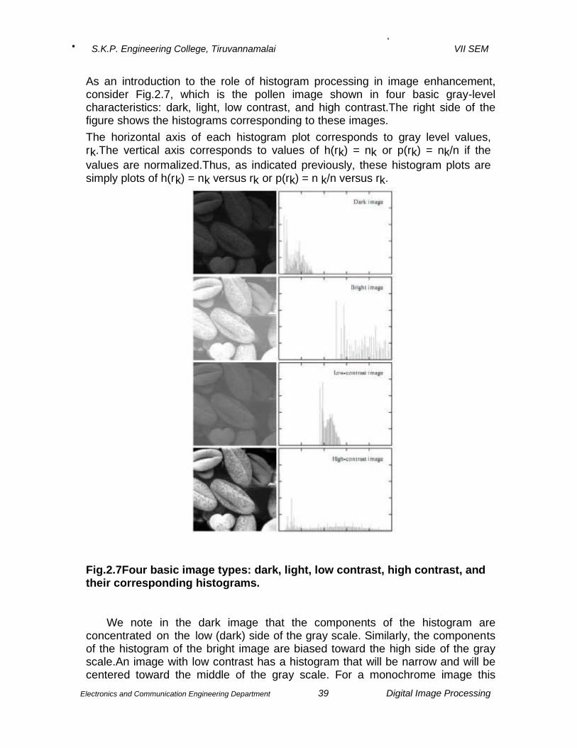
As an introduction to the role of histogram processing in image enhancement, consider Fig.2.7, which is the pollen image shown in four basic gray-level characteristics: dark, light, low contrast, and high contrast.The right side of the figure shows the histograms corresponding to these images. The horizontal axis of each histogram plot corresponds to gray level values, rk.The vertical axis corresponds to values of h(rk) = nk or p(rk) = nk/n if the values are normalized.Thus, as indicated previously, these histogram plots are simply plots of h(rk) = nk versus rk or p(rk) = n k/n versus rk.
Fig.2.7Four basic image types: dark, light, low contrast, high contrast, and their corresponding histograms.
We note in the dark image that the components of the histogram are concentrated on the low (dark) side of the gray scale. Similarly, the components of the histogram of the bright image are biased toward the high side of the gray scale.An image with low contrast has a histogram that will be narrow and will be centered toward the middle of the gray scale. For a monochrome image this
S.K.P. Engineering College, Tiruvannamalai VII SEM
Electronics and Communication Engineering Department 40 Digital Image Processing
implies a dull,washed-out gray look. Finally,we see that the components of the histogram in the high-contrast image cover a broad range of the gray scale and, further, that the distribution of pixels is not too far from uniform,with very few vertical lines being much higher than the others. Intuitively, it is reasonable to conclude that an image whose pixels tend to occupy the entire range of possible gray levels and, in addition, tend to be distributed uniformly,will have an appearance of high contrast and will exhibit a large variety of gray tones. The net effect will be an image that shows a great deal of gray-level detail and has high dynamic range. It will be shown shortly that it is possible to develop a transformation function that can automatically achieve this effect, based only on information available in the histogram of the input image. 4. Write about histogram equalization and specification. [CO1-L1-May/June 2014] [CO1-L1-Nov/Dec 2013]
Histrogram Equalization
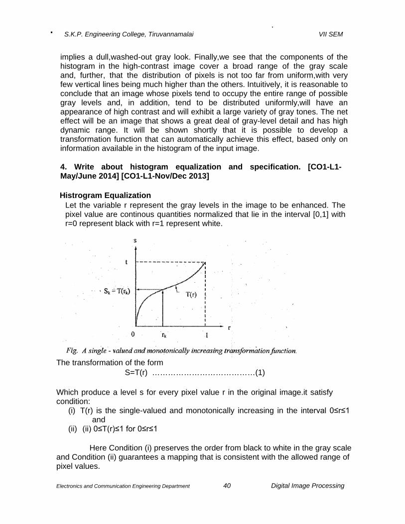
Let the variable r represent the gray levels in the image to be enhanced. The pixel value are continous quantities normalized that lie in the interval [0,1] with r=0 represent black with r=1 represent white.
The transformation of the form S=T(r) …………………………………(1)
Which produce a level s for every pixel value r in the original image.it satisfy condition:
(i) T(r) is the single-valued and monotonically increasing in the interval 0≤r≤1 and
(ii) (ii) 0≤T(r)≤1 for 0≤r≤1
Here Condition (i) preserves the order from black to white in the gray scale and Condition (ii) guarantees a mapping that is consistent with the allowed range of pixel values.

S.K.P. Engineering College, Tiruvannamalai VII SEM
Electronics and Communication Engineering Department 41 Digital Image Processing
R=T-¹(s) 0≤s≤1 ………………………..(2)
The probability density function of the transformed graylevel is Ps(s)=[pr(r)dr/ds] r=T-¹(s) …………….(3)
Consider the transformation function S=T(r)= ∫Pr(w)dw 0≤r≤1 …… (4)
Where w is the dummy variable of integration . From Eqn(4) the derivative of s with respect to r is
ds/dr=pr(r) Substituting dr/ds into eqn(3) yields
Ps(s)=[1] 0≤s≤1 Histogram Specfication
Histogram equalization method does not lent itself to interactive application . Let Pr(r) and Pz(z) be the original and desired probability function. Suppose the histogram equalization is utilized on the original image
S=T(r)=∫Pr(w) dw ………………………………….(5)
Desired image levels could be equalized using the transformation function V=G(z)=∫Pr(w)dw ……………………………..(6)
The inverse process is, z=G-¹(v). Here Ps(s) and Pv(v) are identical uniform densities
Z=G-¹(s) Assume that G-¹(s) is single-valued, the procedure can be summarized as follow
1. Equalize the level of the original image using eqn(4) 2. Specify the desired density function and obtain the transformation function G(z)
using eqn(6) 3. Apply the inverse transformation function Z=G-¹(s) to the level obtained in step
1. we can obtain result in combined transformation function
z=G-¹[T(r)] ……………………………..(7) Histogram specification for digital image is limited one
1. First specify a particular histogram by digitizing the given function. 2. Specifying a histogram shape by means of a graphic device whose
output is fed into the processor executing the histogram specification algorithm.

S.K.P. Engineering College, Tiruvannamalai VII SEM
Electronics and Communication Engineering Department 42 Digital Image Processing
5. Explain Sharpening of spatial filters [CO1-L1] The principle objective of sharpening is to (i)highlight fine detail in an image (ii) enhance detail that has been blurred, either in error or as a natural effect - Since averaging is analogous to integration, it is logical to conclude that sharpening could be accomplished by spatial differentiation. Requirements of Second order derivatives are i) Must be zero in flat areas ii) Must be non zero at the onset and end of a gray level step or ramp iii) Must be zero along ramps of constant slope.
Second order derivatives can be defined as the difference as,
Adding the image to the Laplacian restored the overall gray level variations in the image, with the Laplacian increasing the contrast at the locations of gray-level discontinuities.A process used for many years in the publishing industry to sharpen images consists of subtracting a blurred version of an image from the image itself. Unsharp masking and High-boost filtering: A slight further generalization of unsharp masking is called high-boost filtering. A high-boost filtered image, fhb, is defined at any point (x, y) as
Adding and subtracting f(x,y),
Fig.2.9 3*3 masks used for high boost filtering

S.K.P. Engineering College, Tiruvannamalai VII SEM
Electronics and Communication Engineering Department 43 Digital Image Processing
When A=1, high-boost filtering becomes “standard” Laplacian sharpening.
As the value of A increases past 1, the contribution of the sharpening process becomes less and less important. Eventually, if A is large enough, the high-boost image will be approximately equal to the original image multiplied by a constant. Use of First Derivatives for Enhancement—the Gradient First derivatives in image processing are implemented using the magnitude of the gradient. For a function f(x, y), the gradient of f at coordinates (x, y) is defined as the two-dimensional column vector.
Two important operators to compute the gradient are 1. Roberts cross-gradient operators. 2. Sobel operators Roberts cross-gradient operators Uses cross differences
Sobel operators uses rows and columns operation

S.K.P. Engineering College, Tiruvannamalai VII SEM
Electronics and Communication Engineering Department 44 Digital Image Processing
6. Discuss about the mechanics of filtering in spatial domain. Mention the points to be considered in implementation neighbourhood operations for spatial filtering. [CO1-L1]
Basics of Spatial Filtering: Some neighborhood operations work with the values of the image pixels in the neighborhood and the corresponding values of a subimage that has the same dimensions as the neighborhood.The subimage is called a filter,mask, kernel, template, or window,with the first three terms being the most prevalent terminology.The values in a filter subimage are referred to as coefficients, rather than pixels. The concept of filtering has its roots in the use of the Fourier transform for signal processing in the so-called frequency domain. We use the term spatial filtering to differentiate this type of process from the more traditional frequency domain filtering.
The use of spatial mask for the image processing usually called spatial filtering and spatial mask are spatial filters.
The linear filter classified into o Low pass o High pass o Band pass filtering

S.K.P. Engineering College, Tiruvannamalai VII SEM
Electronics and Communication Engineering Department 45 Digital Image Processing
1 1 1 1 1 1 1 1 1
-1 -1 -1 -1 8 -1 -1 -1 -1
Consider 3*3 mask
W1 W2 W3
W4 W5 W6
W7 W8 W9
Denoting the gray level of pixels under the mask at any location by z1,z2,z3……,z9, the response of a linear mask is
R=w1z1+ w2z2 +………..+w9z9
Smoothing Filters Lowpass Spatial filtering:
The filter has to have positive coefficient. The response would be the sum of gray levels of nine pixels
which could cause R to be out of the gray level range. The solution is to scale the sum by dividing R by 9.The use
of the form of mask are called neighborhood averaging
1/9
Median filtering: To achive noise reduction rather than blurring. The gray level of each pixel is replaced by the median of
the gray level in the neighbourhood of that pixel Sharpening Filters
Basic highpass spatial filtering: The filter should be positive ecoefficient near the center and negative in the outer periphery.(i) The sum of the coefficient are 0.(ii) This eliminate the zero- frequency term reducing significantly the global contrast of the image
1/9*
High_boost filtering: The definition is
High-boost=(A)(Original)-Lowpass =(A-1) (Original)+ Original –Lowpass =(A-1) (Original)+Hignpass
Derivative Filters:Averaging is anlog to integration , differentiation can be expected

S.K.P. Engineering College, Tiruvannamalai VII SEM
Electronics and Communication Engineering Department 46 Digital Image Processing
to have opposite effect and thus sharpen the image 7. Write about Smoothing Spatial filters. [CO1-L1-Nov/Dec 2014]
Smoothing Spatial Filters:
Smoothing filters are used for blurring and for noise reduction. Blurring is used in preprocessing steps, such as removal of small details from an image prior to (large) object extraction, and bridging of small gaps in lines or curves. Noise reduction can be accomplished by blurring with a linear filter and also by non-linear filtering.
((i) Smoothing Linear Filters:
The output (response) of a smoothing, linear spatial filter is simply the average of the pixels contained in the neighborhood of the filter mask. These filters sometimes are called averaging filters. The idea behind smoothing filters is straight forward.By replacing the value of every pixel in an image by the average of the gray levels in the neighborhood defined by the filter mask, this process results in an image with reduced ―sharp‖ transitions in gray levels. Because random noise typically consists of sharp transitions in gray levels, the most obvious application of smoothing is noise reduction.However, edges (which almost always are desirable features of an image) also are characterized by sharp transitions in gray levels, so averaging filters have the undesirable side effect that they blur edges. Another application of this type of process includes the smoothing of false contours that result from using an insufficient number of gray levels.
Fig.2.9 Two 3 x 3 smoothing (averaging) filter masks.The constant multiplier in front of each mask is equal to the sum of the values of its coefficients, as is required to compute an average. Figure 2.9 shows two 3 x 3 smoothing filters. Use of the first filter yields the standard average of the pixels under the mask.This can best be seen by substituting the coefficients of the mask in

S.K.P. Engineering College, Tiruvannamalai VII SEM
Electronics and Communication Engineering Department 47 Digital Image Processing
∑∑
∑∑−= −=
++= a b
a
as
b
bt
tsw
tysxftswyxg
),(
),(),(),(
∑∑
∑∑−= −=
++= a b
a
as
b
bt
tsw
tysxftswyxg
),(
),(),(),(
which is the average of the gray levels of the pixels in the 3 x 3 neighborhood defined by the mask.Note that, instead of being 1/9, the coefficients of the filter are all 1’s.The idea here is that it is computationally more efficient to have coefficients valued 1. At the end of the filtering proce ss the entire image is divided by 9. An m x n mask would have a normalizing constant equal to 1/mn.
A spatial averaging filter in which all coefficients are equal is sometimes called a box filter.The second mask shown in Fig.2.9 is a little more interesting. This mask yields a so-called weighted average, terminology used to indicate that pixels are multiplied by different coefficients, thus giving more importance (weight) to some pixels at the expense of others. The general implementation for filtering an M x N image with a weighted averaging filter of size m x n (m and n odd) is given by the expression
(2) Order-Statistics Filters:
Order-statistics filters are nonlinear spatial filters whose response is based on ordering (ranking) the pixels contained in the image area encompassed by the filter, and then replacing the value of the center pixel with the value determined by the ranking result. The best-known example in this category is the median filter, which, as its name implies, replaces the value of a pixel by the median of the gray levels in the neighborhood of that pixel (the original value of the pixel is included in the computation of the median). Median filters are quite popular because, for certain types of random noise, they provide excellent noise-reduction capabilities, with considerably less blurring than linear smoothing filters of similar size. Median filters are particularly effective in the presence of impulse noise, also called salt-and-pepper noise because of its appearance as white and black dots superimposed on an image.
8. Write short notes on ideal Butterworth and Gaussian Filters[CO1-L1] Smoothing Frequency Domain Filters: Edges and other sharp transition of the gray levels of an image contribute significantly to the high frequency contents of its Fourier transformation. Hence smoothing is achieved in the frequency domain by attenuation a specified range of high frequency components in the transform of a given image. Basic model of filtering in the frequency domain is G(u,v) = H(u,v)F(u,v)

S.K.P. Engineering College, Tiruvannamalai VII SEM
Electronics and Communication Engineering Department 48 Digital Image Processing
F(u,v) - Fourier transform of the image to be smoothed Objective is to find out a filter function H (u,v) that yields G (u,v) by attenuating the high frequency component of F (u,v) There are three types of low pass filters 1. Ideal 2. Butterworth 3. Gaussian IDEAL LOW PASS FILTER It is the simplest of all the three filters.It cuts of all high frequency component of the Fourier transform that are at a distance greater that a specified distance D0 form the origin of the transform. it is called a two –dimensional ideal low pass filter (ILPF) and has the transfer function
Where D0 is a specified nonnegative quantity and D(u,v) is the distance from point (u,v) to the center of frequency rectangle.If the size of image is M*N , filter will also be of the same size so center of the frequency rectangle (u,v) = (M/2, N/2) because of center transform
Because it is ideal case. So all frequency inside the circle are passed without any attenuation whereas all frequency outside the circle are completely attenuated.For an ideal low pass filter cross section, the point of transition between H(u,v) =1 and H(u,v)=0 is called of the “ cut of frequency” BUTTERWORTH LOW PASS FILTER It has a parameter called the filter order.For high values of filter order it approaches the form of the ideal filter whereas for low filter order values it reach Gaussian filter. It may be viewed as a transition between two extremes. The transfer function of a Butterworth low pass filter (BLPF) of order n with cut off frequency at distance Do from the origin is defined as

S.K.P. Engineering College, Tiruvannamalai VII SEM
Electronics and Communication Engineering Department 49 Digital Image Processing
It does not have sharp discontinuity unlike ILPF that establishes a clear cutoff between passed and filtered frequencies.Defining a cutoff frequency is a main concern in these filters. This filter gives a smooth transition in blurring as a function of increasing cutoff frequency. A Butterworth filter of order 1 has no ringing. Ringing increases as a function of filter order. (Higher order leads to negative values)
Fig. ideal Butterworth low pass filter
GAUSSIAN LOW P ASS FILTER:
The transfer function of a Gaussian low pass filter is
Where: D(u,v)- the distance of point (u,v) from the center of the transform σ = D0- specified cut off frequency The filter has an important characteristic that the inverse of it is also Gaussian.

S.K.P. Engineering College, Tiruvannamalai VII SEM
Electronics and communication Engineering Department 92 Digital Image Processing
Unit III
Image Restoration And Segmentation
Part-A
1. Give the relation/PDF for Gaussian noise and Rayleigh noise[CO1-L1-May/June 2013] Gaussian noise: The PDF Gaussian random variable Z is given by
,
Where Z--Gray level value;σ-standard deviation;σ2-variance of Z;
µ-mean of the gray level value Z.
Rayleigh noise: The PDF is
Here ,Mean µ=a+√πb/4; Standard deviation σ2=b(4-π)/4
2. Give the relation for Gamma noise, Exponential noise. [CO1-L1] Gamma noise: The PDF is
Here,Mean µ=b/a; Standard deviation σ2=b/a2
Exponential noise : The PDF is
Here, Mean µ=1/a; Standard deviation σ2=1/a2
3. Give the relation for Uniform noise and Impulse noise[CO1-L1-May/June 2013] Uniform noise:The PDF is

S.K.P. Engineering College, Tiruvannamalai VII SEM
Electronics and communication Engineering Department 93 Digital Image Processing
Mean µ=a+b/2 ; Standard deviation σ2=(b-a)2/12
Impulse noise:The PDF is
4. What are possible ways for adding noise in images? [CO1-L1-Nov/Dec 2013] Image sensors, scanners, image acquisition, modify the pixel values, changing the background or foreground of an image, addition of two images, arithmetic operations between two images and image processing algorithms are the possible ways for adding noise in images. 5. What is meant by Image Restoration? [CO1-L1] Restoration attempts to reconstruct or recover an image that has been degraded by using a clear knowledge of the degrading phenomenon.
6. What is Local threshold and dynamic or adaptive threshold, global thresholding? [CO1- L1-May/June 2013]
If Threshold T depends both on f(x,y) and p(x,y) is called local. If Threshold T depends on the spatial coordinates x and y the threshold is called dynamic or adaptive where f(x,y) is the original image.
7. How a degradation process is modeled? Or Define degradation model and sketch it. [CO1-L1-May/June 2015] [CO1-L1-Nov/Dec 2012]
A system operator H, which together with an additive white noise term η(x,y) operates on an input image f(x,y) to produce a degraded image g(x,y).
8. Define Gray-level interpolation[CO1-L1] Gray-level interpolation deals with the assignment of gray levels to pixels in the spatially transformed image

S.K.P. Engineering College, Tiruvannamalai VII SEM
Electronics and communication Engineering Department 94 Digital Image Processing
9. What is meant by Noise probability density function? [CO1-L1] The spatial noise descriptor is the statistical behavior of gray level values in the noise component of the model. 10. What is geometric transformation? [CO1-L1-May/June 2012] [CO1-L1-Nov/Dec 2015] Transformation is used to alter the co-ordinate description of image. The basic geometric transformations are 1. Image translation 2. Scaling 3. Image rotation
11. What is image translation and scaling? [CO1-L1] Image translation means reposition the image from one co-ordinate location to another along straight line path. Scaling is used to alter the size of the object or image (ie) a co-ordinate system is scaled by a factor.
12. Which is the most frequent method to overcome the difficulty to formulate the spatial relocation of pixels? [CO1-L1]
The point is the most frequent method, which are subsets of pixels whose location in the input (distorted) and output (corrected) imaged is known precisely.
13. What are the three methods of estimating the degradation function? [CO1-L1] 1. Observation 2. Experimentation 3. Mathematical modeling. The simplest approach to restoration is direct inverse filtering, an estimate F^(u,v) of the transform of the original image simply by dividing the transform of the degraded image G^(u,v) by the degradation function.
14. What is pseudo inverse filter? [CO1-L1-Nov/Dec 2013] It is the stabilized version of the inverse filter. For a linear shift invariant system with frequency response H(u,v) the pseudo inverse filter is defined as H-(u,v)=1/(H(u,v) H#0
0 H=0
15. What is meant by least mean square filter or wiener filter? [CO1-L1-Nov/Dec 2012] The limitation of inverse and pseudo inverse filter is very sensitive noise. The wiener filtering is a method of restoring images in the presence of blur as well as noise. 16. What is meant by blind image restoration? What are the two approaches for blind image restoration? [CO1-L1]
S.K.P. Engineering College, Tiruvannamalai VII SEM
Electronics and communication Engineering Department 95 Digital Image Processing
An information about the degradation must be extracted from the observed image either explicitly or implicitly. This task is called as blind image restoration. The two approaches for blind image restoration are 1.Direct measurement 2. Indirect estimation 17. Give the difference between Enhancement and Restoration[CO1-L1] Enhancement technique is based primarily on the pleasing aspects it might present to the viewer. For example: Contrast Stretching. Whereas Removal of image blur by applying a deblurrings function is considered a restoration technique. 18. What do you mean by Point processing? [CO1-L1] Image enhancement at any Point in an image depends only on the gray level at that point is often referred to as Point processing. 19. What is Image Negatives? Give the formula for negative and log transformation. [CO1-L1] The negative of an image with gray levels in the range [0, L-1] is obtained by using the negative transformation, which is given by the expression. S=L-1-r; Log Transformation: S = c log(1+r) Where c-constant and ≥0
20.What is meant by bit plane slicing? [CO1-L1-Nov/Dec 2013] Instead of highlighting gray level ranges, highlighting the contribution made to total image appearance by specific bits might be desired. Suppose that each pixel in an image is represented by 8 bits. Imagine that the image is composed of eight 1-bit planes, ranging from bit plane 0 for LSB to bit plane-7 for MSB.
21. Why blur is to be removed from images? [CO1-L1-Nov/Dec 2014]
The blur is caused by lens that is improper manner, relative motion between camera and scene and atmospheric turbulence. It will introduce bandwidth reduction and make the image analysis as complex. To prevent the issues, blur is removed from the images.
22. What is Lagrange multiplier? Where it is used? [CO1-L1-Nov/Dec 2014]
The Lagrange multiplier is a strategy for finding the local minima and maxima of a function subject to equality constraints. This is mainly used in the image restoration process like image acquisition, image storage and transmission.

S.K.P. Engineering College, Tiruvannamalai VII SEM
Electronics and communication Engineering Department 96 Digital Image Processing
23. Compare constrained and unconstrained restoration[CO1-L2-May/June 2014]
Constrained Restoration Unconstrained Restoration
In the absence of any knowledge about the noise ‘n’, based on Lagrange multiplier and linear operator, a meaningful criterion function is to
seek an such that H approximates of in a least square sense by assuming the noise term is as small as possible. Where H = system operator.
= estimated input image.
g = degraded image.
In the absence of any knowledge about the noise ‘n’, a meaningful
criterion function is to seek an such
that H approximates of in a least square sense by assuming the noise term is as small as possible. Where H
= system operator. = estimated input image.
g = degraded image.
24.What is the principle of inverse filtering? [CO1-L1-May/June 2014]
Inverse filtering is given by
-restored image. G(u,v) – Degraded image H(u,v)-Filter transfer function
25. Define rubber sheet transformation[CO1-L1-May/June 2013] Geometric transformations may be viewed as the process of printing an image on a rubber sheet and then stretching the sheet according to some predefined set of rules .Therefore they are also called as rubber sheet transformations. 26. What is segmentation? Write the applications of segmentation. [CO1-L1-Nov/Dec 2013] Segmentation is the process of portioning an image into its constitute regions or objects based on certain criteria. Image segmentation algorithms are based on either discontinuity principle or similarity principle.
* Detection of isolated points. * Detection of lines and edges in an image.

S.K.P. Engineering College, Tiruvannamalai VII SEM
Electronics and communication Engineering Department 97 Digital Image Processing
27. What is edge? What are the two properties used for establishing similarity of edge pixels? [CO1-L1-Nov/Dec 2013] An edge is a set of connected pixels that lie on the boundary between two regions edges are more closely modeled as having a ramp like profile. The slope of the ramp is inversely proportional to the degree of blurring in the edge. Properties used for establishing similarity of edge pixels :(1) The strength of the response of the gradient operator used to produce the edge pixel. (2) The direction of the gradient
28. Define region growing .Give the principle of region growing[CO1-L1-Nov/Dec 2015] Region growing is a procedure that groups pixels or subregions in to layer regions based on predefined criteria. The basic approach is to start with a set of seed points and from there grow regions by appending to each seed these neighboring pixels that have properties similar to the seed.
29. State the problems in region splitting and merging based image segmentation. [CO1-L1-Nov/Dec 2014]
• Initial seed points – different set of initial seed point cause different segmented result.
• Time consuming problem • This method is not suitable for color images and produce fault colors sometime. • Region growth may stop at any time when no more pixels satisfy the criteria.
30. What are factors affecting the accuracy of region growing? [CO1-L1-May/June 2014]
The factors affecting the accuracy of region growing are like lightning variations, pixel’s intensity value.
31. Write sobel horizontal and vertical edge detection masks. [CO1-L1-May/June 2014]

S.K.P. Engineering College, Tiruvannamalai VII SEM
Electronics and communication Engineering Department 98 Digital Image Processing
Horizontal masking Vertical masking
32. Define region splitting and merging. Specify the steps involved in splitting and merging
[CO1-L1-May/June 2014] [CO1-L1-May/June 2014]
Region splitting and merging is a segmentation process in which an image is initially subdivided into a set of arbitrary ,disjoint regions and then the regions are merger and /or splitted to satisfy the basic conditions.
Split into 4 disjoint quadrants any region Ri for which P(Ri)=FALSE. Merge any adjacent regions Rj and Rk for which P(RjURk)=TRUE. Stop when no further merging or splitting is positive.
33. Define and give the transfer function of mean and geometric mean filter[CO1-L1-May/June 2015]
The arithmetic mean filter is a very simple one and is calculated as follows:
The transfer function of Geometric mean filter is
Each restored pixel value given by the product of all the pixel values in the filter window, raised to the power 1/mn. Achieving smoothing comparable to the arithmetic mean filter, but tending to lose less image detail in the process
-1 0 1
-2 0 2
-1 0 1
-1 -2 -1
0 0 0
1 2 2
mn
Sts xy
tsgyxf
1
),(
),(),(ˆ
= ∏
∈
∑∈
=xySts
tsgmn
yxf),(
),(1),(ˆ

S.K.P. Engineering College, Tiruvannamalai VII SEM
Electronics and communication Engineering Department 99 Digital Image Processing
PART-B
1.Write about various Noise Probability Density Functions. [CO1-L1-May/June 2010] The following are among the most common PDFs found in image processing applications. Gaussian noise Because of its mathematical tractability in both the spatial and frequency domains, Gaussian (also called normal) noise models are used frequently in practice. In fact, this tractability is so convenient that it often results in Gaussian models being used in situations in which they are marginally applicable at best.
The PDF Gaussian random variable Z is given by
where z represents gray level, μ is the mean of average value of z, and a σ is its standard deviation. The standard deviation squared, σ2, is called the variance of z. A plot of this function is shown in Fig. 3.1. When z is described by Eq. (1), approximately 70% of its values will be in the range [(μ - σ), (μ +σ)], and about 95% will be in the range [(μ - 2σ), (μ + 2σ)].
Fig.3.1 A plot of this function of Gaussian noise
Rayleigh noise
The PDF of Rayleigh noise is given by
Here ,Mean µ=a+√πb/4; Standard deviation σ2=b(4-π)/4

S.K.P. Engineering College, Tiruvannamalai VII SEM
Electronics and communication Engineering Department 100 Digital Image Processing
Figure3.2 shows a plot of the Rayleigh density. Note the displacement from the origin and the fact that the basic shape of this density is skewed to the right. The Rayleigh density can be quite useful for approximating skewed histograms.
Fig.3.2 A plot of this function of Rayleigh noise
Erlang (Gamma) noise
The PDF of Erlang noise is given by
Here,Mean µ=b/a; Standard deviation σ2=b/a2
Exponential noise
The PDF of exponential noise is given by

S.K.P. Engineering College, Tiruvannamalai VII SEM
Electronics and communication Engineering Department 101 Digital Image Processing
Here, Mean µ=1/a; Standard deviation σ2=1/a2
This PDF is a special case of the Erlang PDF, with b = 1.
Uniform noise
The PDF of uniform noise is given by
Here, Mean µ=a+b/2 ; Standard deviation σ2=(b-a)2/12
Impulse (salt-and-pepper) noise
The PDF of (bipolar) impulse noise is given by
If b > a, gray-level b will appear as a light dot in the image. Conversely, level a will appear like a dark dot.If either Pa or Pb is zero, the impulse noise is called unipolar. If neither probability is zero, and especially if they are approximately equal, impulse noise values will resemble salt-and-pepper granules randomly distributed over the image. For this reason, bipolar impulse noise also is called salt-and-pepper noise. Shot and spike noise also are terms used to refer to this type of noise.Fig 3.3 shows different plot function of different types of noise.

S.K.P. Engineering College, Tiruvannamalai VII SEM
Electronics and communication Engineering Department 102 Digital Image Processing
Fig.3.3 plot function of Gamma, Exponential, Uniform, Impulse noise.
2.Explain various Mean filters. [CO1-L1]
There are four types of mean filters. They are
(i) Arithmetic mean filter
This is the simplest of the mean filters. Let Sxy represent the set of coordinates in a rectangular subimage window of size m X n, centered at point (x, y).The arithmetic mean filtering process computes the average value of the corrupted image g(x, y) in the area defined by Sxy. The value of the restored image f at any point (x, y) is simply the arithmetic mean computed using the pixels in the region defined by Sxy.

S.K.P. Engineering College, Tiruvannamalai VII SEM
Electronics and communication Engineering Department 103 Digital Image Processing
This operation can be implemented using a convolution mask in which all coefficients have value 1/mn.
(ii) Geometric mean filter
An image restored using a geometric mean filter is given by the expression
Here, each restored pixel is given by the product of the pixels in the subimage window, raised to the power 1/mn. A geometric mean filter achieves smoothing comparable to the arithmetic mean filter, but it tends to lose less image detail in the process.
(iii) Harmonic mean filter (Nov 2014)
The harmonic mean filter works well for salt noise, but fails for pepper noise. It does well also with other types of noise like Gaussian noise.
(iv) Contra harmonic mean filter
This filter is well suited for reducing or virtually eliminating the effects of salt-and-pepper noise. For positive values of Q, the filter eliminates pepper noise. For negative values of Q it eliminates salt noise. It cannot do both simultaneously.
Note that the contra harmonic filter reduces to the arithmetic mean filter if Q = 0, and to the harmonic mean filter if Q = -1.
3. Explain the Order-Statistic Filters. [CO1-L1]
There are four types of Order-Statistic filters. They are
(i) Median filter The best-known order-statistics filter is the median filter, which, as its name implies, replaces the
value of a pixel by the median of the gray levels in the neighborhood of that pixel:
Median {g(s,t)}
The original value of the pixel is included in the computation of the median. Median filters are quite popular because, for certain types of random noise, they provide

S.K.P. Engineering College, Tiruvannamalai VII SEM
Electronics and communication Engineering Department 104 Digital Image Processing
excellent noise-reduction capabilities, with considerably less blurring than linear smoothing filters of similar size. Median filters are particularly effective in the presence of both bipolar and unipolar impulse noise.
(ii) Max and min filters
Although the median filter is by far the order-statistics filler most used in image processing, it is by no means the only one. The median represents the 50th percentile of a ranked set of numbers, but the reader will recall from basic statistics that ranking lends itself to many other possibilities. For example, using the 100th percentile results in the so-called max filter, given by
max{g(s,t)}
This filter is useful for finding the brightest points in an image. Also, because pepper noise has very low values, it is reduced by this filter as a result of the max selection process in the subimage area Sxy.
(iii) Alpha - trimmed mean filter
It is a filter formed by deleting the d/2 lowest and the d/2 highest gray-level values of g(s, t) in the neighborhood Sxy. Let gr (s, t) represent the remaining mn - d pixels. A filter formed by averaging these remaining pixels is called an alpha-trimmed mean filter:
where the value of d can range from 0 to mn - 1. When d = 0, the alpha- trimmed filter reduces to the arithmetic mean filter. If d = (mn - l)/2, the filter becomes a median filter. For other values of d, the alpha-trimmed filter is useful in situations involving multiple types of noise, such as a combination of salt-and-pepper and Gaussian noise.

S.K.P. Engineering College, Tiruvannamalai VII SEM
Electronics and communication Engineering Department 105 Digital Image Processing
4. Explain the Adaptive Filters. [CO1-L1]
Adaptive filters are filters whose behavior changes based on statistical characteristics of the image inside the filter region defined by the m X n rectangular window Sxy.
Adaptive, local noise reduction filter:
The simplest statistical measures of a random variable are its mean and variance. These are reasonable parameters on which to base an adaptive filler because they are quantities closely related to the appearance of an image. The mean gives a measure of average gray level in the region over which the mean is computed, and the variance gives a measure of average contrast in that region.This filter is to operate on a local region, Sxy. The response of the filter at any point (x, y) on which the region is centered is to be based on four quantities: (a) g(x, y), the value of the noisy image at (x, y); (b) a2, the variance of the noise corrupting (x, y) to form g(x, y); (c) ray,the local mean of the pixels in Sxy; and (d) σ2 L , the local variance of the pixels in Sxy.The behavior of the filter to be as follows:
1. If σ2 η is zero, the filler should return simply the value of g (x, y). This is the trivial, zero-noise case in which g(x, y) is equal to f (x, y).
2. If the local variance is high relative to σ2η the filter should return a value close to g (x, y). A high local variance typically is associated with edges, and these should be preserved.
3. If the two variances are equal, we want the filter to return the arithmetic mean value of the pixels in Sxy.This condition occurs when the local area has the same properties as the overall image, and local noise is to be reduced simply by averaging.
Adaptive local noise filter is given by,
The only quantity that needs to be known or estimated is the variance of the overall noise, a2. The other parameters are computed from the pixels in Sxy at each location (x, y) on which the filter window is centered.
Adaptive median filter:
The median filter performs well as long as the spatial density of the impulse noise is not large (as a rule of thumb, Pa and Pb less than 0.2). The adaptive median

S.K.P. Engineering College, Tiruvannamalai VII SEM
Electronics and communication Engineering Department 106 Digital Image Processing
filtering can handle impulse noise with probabilities even larger than these. An additional benefit of the adaptive median filter is that it seeks to preserve detail while smoothing nonimpulse noise, something that the "traditional" median filter does not do. The adaptive median filter also works in a rectangular window area Sxy. Unlike those filters, however, the adaptive median filter changes (increases) the size of Sxy during filter operation, depending on certain conditions. The output of the filter is a single value used to replace the value of the pixel at (x, y), the particular point on which the window Sxy is centered at a given time.
Consider the following notation:
zmin = minimum gray level value in Sxy
zmax = maximum gray level value in Sxy
zmcd = median of gray levels in Sxy
zxy = gray level at coordinates (x, y)
Smax = maximum allowed size of Sxy.
The adaptive median filtering algorithm works in two levels, denoted level A and level B, as
follows:
Level A: A1 = zmed - zmin
A2 = zmed - zmax If A1 > 0 AND A2 < 0,
Go to level B Else increase the window size
If window size ≤ Smax repeat level A
Else output zxy
Level B: B1 = zxy - zmin
B2 = zxy - zmax
If B1> 0 AND B2 < 0, output zxy
Else output zmed
S.K.P. Engineering College, Tiruvannamalai VII SEM
Electronics and communication Engineering Department 107 Digital Image Processing
5. Write brief notes on inverse filtering. [CO1-L1-May/June 2010] [CO1-L1-Nov/Dec 2012]
The simplest approach to restoration is direct inverse filtering, where F (u, v), the transform of the original image is computed simply by dividing the transform of the degraded image, G (u,v), by the degradation function
The divisions are between individual elements of the functions. But G (u,v) is given by
G (u, v) = F (u, v) + N (u, v)
It tells that even if the degradation function is known the undegraded image cannot be recovered [the inverse Fourier transform of F( u, v)] exactly because N(u, v) is a random function whose Fourier transform is not known.If the degradation has zero or very small values, then the ratio N(u, v)/H(u, v) could easily dominate the estimate F(u, v).One approach to get around the zero or small-value problem is to limit the filter frequencies to values near the origin. H (0, 0) is equal to the average value of h(x, y) and that this is usually the highest value of H (u, v) in the frequency domain. Thus, by limiting the analysis to frequencies near the origin, the probability of encountering zero values is reduced.
6. Explain the various noise reduction filters. [CO1-L1]
The basic idea is that periodic noise appears as concentrated bursts of energy in the Fourier transform, at locations corresponding to the frequencies of the periodic interference. The approach is to use a selective filter to isolate the noise.The three types of selective filters bandreject, bandpass, and notch are used for basic periodic noise reduction. Band reject Filters One of the principal applications of bandreject filtering is for noise removal in applications where the general location of the noise component(s) in the frequency domain is approximately known. A good example is an image corrupted by additive periodic noise that can be approximated as two-dimensional sinusoidal functions. It is not difficult to show that the Fourier transform of a sine consists of two impulses that are mirror images of each other about the origin of the transform.The impulses are both
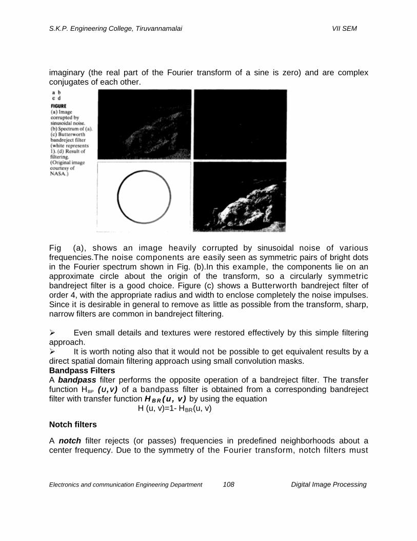
S.K.P. Engineering College, Tiruvannamalai VII SEM
Electronics and communication Engineering Department 108 Digital Image Processing
imaginary (the real part of the Fourier transform of a sine is zero) and are complex conjugates of each other.
Fig (a), shows an image heavily corrupted by sinusoidal noise of various frequencies.The noise components are easily seen as symmetric pairs of bright dots in the Fourier spectrum shown in Fig. (b).In this example, the components lie on an approximate circle about the origin of the transform, so a circularly symmetric bandreject filter is a good choice. Figure (c) shows a Butterworth bandreject filter of order 4, with the appropriate radius and width to enclose completely the noise impulses. Since it is desirable in general to remove as little as possible from the transform, sharp, narrow filters are common in bandreject filtering. Even small details and textures were restored effectively by this simple filtering approach. It is worth noting also that it would not be possible to get equivalent results by a direct spatial domain filtering approach using small convolution masks. Bandpass Filters A bandpass filter performs the opposite operation of a bandreject filter. The transfer function HBP (U,V) of a bandpass filter is obtained from a corresponding bandreject filter with transfer function H B R (u , v ) by using the equation H (u, v)=1- HBR(u, v)
Notch filters
A notch filter rejects (or passes) frequencies in predefined neighborhoods about a center frequency. Due to the symmetry of the Fourier transform, notch filters must

S.K.P. Engineering College, Tiruvannamalai VII SEM
Electronics and communication Engineering Department 109 Digital Image Processing
appear in symmetric pairs about the origin in order to obtain meaningful results. The one exception to this rule is if the notch filter is located at the origin, in which case it appears by itself.Although we show only one pair for illustrative purposes, the number of pairs of notch filters that can be implemented is arbitrary. The shape of the notch areas also can be arbitrary (e.g., rectangular). We can obtain notch filters that pass, rather than suppress, the frequencies contained in the notch areas.Since these filters perform exactly the opposite function as the notch reject filters.where HNP(u,v) is the transfer function of the notch pass filter corresponding to the notch reject filter with transfer function HNR(u, v ) . Optimum Notch Filtering
Alternative filtering methods that reduce the effect of these degradations are quite useful in many applications. The method discussed here is optimum, in the sense that it minimizes local variances of the restored estimate f (x , y ) .The procedure consists of first isolating the principal contributions of the interference pattern and then subtracting a variable, weighted portion of the pattern from the corrupted image. Although we develop the procedure in the context of a specific application, the basic approach is quite general and can be applied to other restoration tasks in which multiple periodic interference is a problem.The first step is to extract the principal frequency components of the interference pattern. As before, this can be done by placing a notch pass filter. H N P (u , v ) , at the location of each spike. If the filter is constructed to pass only-components associated with the interference pattern, then the Fourier transform of the interference noise pattern is given by the expression N (u, v)= HNP (u, v) G(u, v) where, as usual, G(u, v), denotes the Fourier transform of the corrupted image. Formation of H NP (u,v ) requires considerable judgment about what is or is not an interference spike.For this reason, the notch pass filter generally is constructed interactively by observing the spectrum of G (u,v ) on a display. Because the corrupted image is assumed to be formed by the addition of the uncorrupted image f ( x , y) and the interference, if ŋ(x, y) were known completely, subtracting (he pattern from g(x , y) to obtain f(x, y) would be a simple matter. The problem, of course, is that (his filtering procedure usually yields only an approximation of the true pattern.

S.K.P. Engineering College, Tiruvannamalai VII SEM
Electronics and communication Engineering Department 110 Digital Image Processing
7.What is Wiener filter? Mention its importance. [CO1-L1-May/June 2011] [CO1-L1-Nov/Dec 2012]
The most important technique for removal of blur in images due to linear motion or unfocussed optics is the Wiener filter. From a signal processing standpoint, blurring due to linear motion in a photograph is the result of poor sampling. Each pixel in a digital representation of the photograph should represent the intensity of a single stationary point in front of the camera. Unfortunately, if the shutter speed is too slow and the camera is in motion, a given pixel will be an amalgram of intensities from points along the line of the camera's motion. This is a two-dimensional analogy to
G(u,v)=F(u,v).H(u,v)
where F is the fourier transform of an "ideal" version of a given image, and H is the blurring function. In this case H is a sinc function: if three pixels in a line contain info from the same point on an image, the digital image will seem to have been convolved with a three-point boxcar in the time domain. Ideally one could reverse-engineer a Fest, or F estimate, if G and H are known. This technique is inverse fitering.
It should be noted that the image restoration tools described here work in a similar manner for cases with blur due to incorrect focus. In this case the only difference is in the selection of H. The 2-d Fourier transform of H for motion is a series of sinc functions in parallel on a line perpendicular to the direction of motion; and the 2-d Fourier transform of H for focus blurring is the sombrero function, described elsewhere.
In the real world, however, there are two problems with this method. First, H is not known precisely. Engineers can guess at the blurring function for a given circumstance, but determination of a good blurring function requires lots of trial and error. Second, inverse filtering fails in some circumstances because the sinc function goes to 0 at some values of x and y. Real pictures contain noise which becomes amplified to the point of destroying all attempts at reconstruction of an Fest.
The best method to solve the second problem is to use Wiener filtering. This tool solves an estimate for F according to the following equation:

S.K.P. Engineering College, Tiruvannamalai VII SEM
Electronics and communication Engineering Department 111 Digital Image Processing
Advantages of Wiener filtering over inverse filtering:
(i). Wiener filtering has no zero or small value problem.
(ii). The results obtained in Wiener filtering are more closer to the original image than inverse filtering.
Disadvantages: It requires power spectrum of ungraded image of noise to be known which makes the implementation more difficult.
8.Explain in detail about the process of edge linking and boundary detection? (May/June-2013)
Linking the edges of an image is done by edge linking and boundary detection.
The following techniques are used for edge linking and boundary detection. 1). Local processing. 2). Global processing using Hough transform. 3). Global processing using graph theoretic approach. 1) Local processing:- One method for linking edges is to analyze the characteristic pixel in small neighborhood about every point in an image.Two properties in this analysis are: (i). the strength of the response of gradient operator used to produce the edge pixel. (ii). the direction of gradient vector. 2) Global processing via Hough transform[CO1-L1-May/June 2015] Edge linking via hough transform: In this method, global relationship between pixel are considered and the points are linked by first determined whether they lie on a curve (or) a specified shape Let there are n-points in an image if the subset of points that lie on the straight line are to be found.Consider a point xi, yi the general equation of straight line.yi = axi + b.now the number of lines passed through the xi and yi for different values of a and b. let to consider a second point xi, yi also has a line. Let this line intercept the line (xi, yi ).There are ‘n’ points in an image. We have to find the subsets of points that lie on standard lines.

S.K.P. Engineering College, Tiruvannamalai VII SEM
Electronics and communication Engineering Department 112 Digital Image Processing
One possible solution is to first find all lines. Consider a point (xi, yi) and general equation of a standard line in slope – intercept form. yi = axi + b Infinitely many lines past through (xi, yi) but all satisfy the equation yi = axi + b For varying a & b. However writing this equation as b= -axi + yi and considering ab plane yields the equation of a single line for fixed pair (x i, y i). Further a second point (x i , y i ) also has a lines in parameter space associated with it and this line intersects the line associated with (x i , y i ) at (a’, b’)
The computational bmin attractiveness bmax of the Hough transform arises from subdividing the parameter space into Accumulator cells.
y b’
S.K.P. Engineering College, Tiruvannamalai VII SEM
Electronics and communication Engineering Department 113 Digital Image Processing
9. Explain the principle of Region splitting and merging in details. [CO1-L1-May/June 2013] [CO1-L1-Nov/Dec 2010]
Region-Based Segmentation:
The objective of segmentation is to partition an image into regions. We approached this problemby finding boundaries between regions based on discontinuities in gray levels, whereas segmentation was accomplished via thresholds based on the distribution of pixel properties, such as gray-level values or color.
Basic Formulation:
Let R represent the entire image region. We may view segmentation as a process that partitions R into n subregions, R1, R 2..., Rn, such that The predicate P(Ri) is used to check the condition. In any region, if P(Ri)= true, then image is subdivided into various subimages. If P(Ri) = false, then divide the image into quadrants. If P(Ri) = false, then further divide the quadrants into sub quadrants
Region Growing:
As its name implies, region growing is a procedure that groups pixels or subregions into larger regions based on predefined criteria. The basic approach is to start with a set of "seed" points and from these grow regions by appending to each seed those neighboring pixels that have properties similar to the seed (such as specific ranges of gray level or color). When a priori information is not available, the procedure is to compute at every pixel the same set of properties that ultimately will be used to assign pixels to regions during the growing process. If the result of these computations shows clusters of values, the pixels whose properties place them near the centroid of these clusters can be used as seeds.
The selection of similarity criteria depends not only on the problem under consideration, but also on the type of image data available. For example, the analysis of land-use satellite imagerydepends heavily on the use of color. This problem would be significantly more difficult, or even impossible, to handle without the inherent information available in color images. When the images are monochrome, region analysis must be carried out with a set of descriptors based on gray levels and spatial properties (such as moments or texture).
Basically, growing a region should stop when no more pixels satisfy the criteria for inclusion in that region. Criteria such as gray level, texture, and color, are local in nature and do not take into account the "history" of region growth. Additional criteria that increase the power of a region growing algorithm utilize the concept of size, likeness between a candidate pixel and the pixels grown so far (such as a comparison of the gray level of a candidate and the average gray level of the grown region), and the shape

S.K.P. Engineering College, Tiruvannamalai VII SEM
Electronics and communication Engineering Department 114 Digital Image Processing
of the region being grown. The use of these types of descriptors is based on the assumption that a model of expected results is at least partially available.
Region Splitting and Merging:
The procedure just discussed grows regions from a set of seed points. An alternative is to subdivide an image initially into a set of arbitrary, disjointed regions and then merge and/or split the regions in an attempt to satisfy the conditions. A split and merge algorithm that iteratively works toward satisfying these constraints is developed.
Let R represent the entire image region and select a predicate P. One approach for segmenting R is to subdivide it successively into smaller and smaller quadrant regions so that, for any region Ri, P(Ri) = TRUE. We start with the entire region. If P(R) = FALSE, we divide the image into quadrants. If P is FALSE for any quadrant, we subdivide that quadrant into subquadrants, and so on. This particular splitting technique has a convenient representation in the form of a so-called quadtree (that is, a tree in which nodes have exactly four descendantsNote that the root of the tree corresponds to the entire image and that each node corresponds to a
subdivision. In this case, only R4 was subdivided further.
If only splitting were used, the final partition likely would contain adjacent regions with identical properties. This drawback may be remedied by allowing merging, as well as splitting. Satisfying the constraints, requires merging only adjacent regions whose
S.K.P. Engineering College, Tiruvannamalai VII SEM
Electronics and communication Engineering Department 115 Digital Image Processing
combined pixels satisfy the predicate P. That is, two adjacent regions Rj and R k are merged only if P (Rj U Rk) = RUE.
The preceding discussion may be summarized by the following procedure, in which, at any step we
1. Split into four disjoint quadrants any region Ri, for which P (Ri) = FALSE.
2. Merge any adjacent regions Rj and Rk for which P (Rj U Rk) = TRUE.
3. Stop when no further merging or splitting is possible.
Several variations of the preceding basic theme are possible. For example, one possibility is to split the image initially into a set of blocks. Further splitting is carried out as described previously, but merging is initially limited to groups of four blocks that are descendants in the quadtree representation and that satisfy the predicate P. When no further mergings of this type are possible, the procedure is terminated by one final merging of regions satisfying step 2. At this point, the merged regions may be of different sizes. The principal advantage of this approach is that it uses the same quadtree for splitting and merging, until the final merging step.
10. Explain Erosion and Dilation in morphological processing. [CO1-L1] These operations are fundamental to morphological processing. (i) Erosion: With A and B as sets in Z2, the erosion of A by B, denoted A Ɵ B, is defined as
In words, this equation indicates that the erosion of A by B is the set of all points z such that B, translated by z , is contained in A. In the following discussion, set B is assumed to be a structuring element. The statement that B has to be contained in A is equivalent to B not sharing any common elements with the background; we can express erosion in the following equivalent form:
where, Ac is the complement of A and Ø is the empty set.

S.K.P. Engineering College, Tiruvannamalai VII SEM
Electronics and communication Engineering Department 116 Digital Image Processing
The elements of A and B are shown shaded and the background is white. The solid boundary in Fig. (c) is the limit beyond which further displacements of the origin of B would cause the structuring element to cease being completely contained in A.Thus, the locus of points (locations of the origin of B) within (and including) this boundary, constitutes the erosion of A by B. We show the erosion shaded in Fig. (c).The boundary of set A is shown dashed in Figs. (c) and (e) only as a reference; it is not part of the erosion operation. Figure (d) shows an elongated structuring element, and Fig. (e) shows the erosion of A by this element. Note that the original set was eroded to a line.However, these equations have the distinct advantage over other formulations in that they are more intuitive when the structuring element B is viewed as a spatial mask
Thus erosion shrinks or thins objects in a binary image. In fact, we can view erosion as a morphological filtering operation in which image details smaller than the structuring element are filtered (re-moved) from the image. (ii) Dilation However, the preceding definitions have a distinct advantage over other formulations in that they are more intuitive when the structuring element B is viewed as a convolution mask. The basic process of flipping (rotating) B about its origin and then successively displacing it so that it slides over set (image) A is analogous to spatial convolution.Keep in mind, however, that dilation is based on set operations and

S.K.P. Engineering College, Tiruvannamalai VII SEM
Electronics and communication Engineering Department 117 Digital Image Processing
therefore is a nonlinear operation, whereas convolution is a linear operation.Unlike erosion, which is a shrinking or thinning operation, dilation "grows" or "thickens" objects in a binary image. The specific manner and extent of this thickening is controlled by the shape of the structuring element used. In the following Figure (b) shows a structuring element (in this case B = B because the SE is symmetric about its origin). The dashed line in Fig. (c) shows the original set for reference, and the solid line shows the limit beyond which any further displacements of the origin of B by z would cause the intersection of B and A to be empty. Therefore, all points on and inside this boundary constitute the dilation of A by B.Figure (d) shows a structuring element designed to achieve more dilation vertically than horizontally, and Fig. (e) shows the dilation achieved with this element

S.K.P. Engineering College, Tiruvannamalai VII SEM
Electronics and communication Engineering Department 118 Digital Image Processing
Unit IV
Wavelets And Image Compression
Part-A
1. What is image compression? [CO1-L1] Image compression refers to the process of redundancy amount of data required to represent the given quantity of information for digital image. The basis of reduction process is removal of redundant data.
2. What is Data Compression? [CO1-L1]
Data compression requires the identification and extraction of source redundancy. In other words, data compression seeks to reduce the number of bits used to store or transmit information.
3.What are two main types of Data compression? [CO1-L1]
Lossless compression can recover the exact original data after compression. It is used mainly for compressing database records, spreadsheets or word processing files, where exact replication of the original is essential. 1. Lossy compression will result in a certain loss of accuracy in exchange for a
substantial increase in compression. Lossy compression is more effective when used to compress graphic images and digitized voice where losses outside visual or aural perception can be tolerated 4. What are different Compression Methods? [CO1-L1]
Run Length Encoding (RLE) Arithmetic coding Huffman coding and Transform coding 5. Define coding redundancy[CO1-L1-Nov/Dec 2015] If the gray level of an image is coded in a way that uses more code words than necessary to represent each gray level, then the resulting image is said to contain coding redundancy. 6. Define interpixel redundancy. [CO1-L1] The value of any given pixel can be predicted from the values of its neighbors. The information carried by is small. Therefore the visual contribution of a single pixel to an

S.K.P. Engineering College, Tiruvannamalai VII SEM
Electronics and communication Engineering Department 119 Digital Image Processing
image is redundant. Otherwise called as spatial redundant geometric redundant or interpixel redundant. Eg: Run length coding 7. What is run length coding? [CO1-L1-May/June 2015] [CO1-L1-Nov/Dec 2012] Run-length Encoding or RLE is a technique used to reduce the size of a repeating string of characters. This repeating string is called a run; typically RLE encodes a run of symbols into two bytes, a count and a symbol. RLE can compress any type of data regardless of its information content, but the content of data to be compressed affects the compression ratio. Compression is normally measured with the compression ratio: 8. Define compression ratio. [CO1-L1-May/June 2012] Compression Ratio = original size / compressed size 9. Define psycho visual redundancy. [CO1-L1] In normal visual processing certain information has less importance than other information. So this information is said to be psycho visual redundant.
10. Compare lossy and lossless compression technique [CO1-L1-May/June 2014]
In terms of storage, the capacity of a storage device can be effectively increased with methods that compress a body of data on its way to a storage device and decompress it when it is retrieved.
1. In terms of communications, the bandwidth of a digital communication link can be effectively increased by compressing data at the sending end and decompressing data at the receiving end.
2. At any given time, the ability of the Internet to transfer data is fixed. Thus, if data can effectively be compressed wherever possible, significant improvements of data throughput can be achieved. Many files can be combined into one compressed document making sending easier.
Lossless compression technique Lossy compression technique
*In lossless data compression, the integrity of the data is preserved. The original data and the data after compression and decompression are exactly the same because, in these methods, the compression and decompression algorithms are exact inverses of each other: no part of the
*Our eyes and ears cannot distinguish subtle changes. In such cases, we can use a lossy data compression method.
*These methods are cheaper—they take less time and space when it comes to sending millions of bits per

S.K.P. Engineering College, Tiruvannamalai VII SEM
Electronics and communication Engineering Department 120 Digital Image Processing
data is lost in the process. *Redundant data is removed in compression and added during decompression.
*Lossless compression methods are normally used when we cannot afford to lose any data.
*Some techniques are run-length encoding, Huffman coding, Lempel Ziv encoding
second for images and video.
*Several lossy compression techniques are JPEG (Joint Photographic Experts Group) encoding is used to compress pictures and graphics, MPEG (Moving Picture Experts Group) encoding is used to compress video, and MP3 (MPEG audio layer 3) for audio compression
11. Define encoder[CO1-L1] Source encoder is responsible for removing the coding and interpixel redundancy and psycho visual redundancy. There are two components A) Source Encoder B) Channel Encoder
12. Define channel encoder. [CO1-L1]
The channel encoder reduces the impact of the channel noise by inserting redundant bits into the source encoded data. Eg: Hamming code
13. What are the operations performed by error free compression? [CO1-L1] 1) Devising an alternative representation of the image in which its interpixel redundant are reduced. 2) Coding the representation to eliminate coding redundancy
14. What is Variable Length Coding? [CO1-L1] Variable Length Coding is the simplest approach to error free compression. It reduces only the coding redundancy. It assigns the shortest possible codeword to the most probable gray levels. 15. Define Huffman coding and mention its limitation [CO1-L1-May/June 2012] [CO1-L1-Nov/Dec 2013] 1. Huffman coding is a popular technique for removing coding redundancy. 2. When coding the symbols of an information source the Huffman code yields

S.K.P. Engineering College, Tiruvannamalai VII SEM
Electronics and communication Engineering Department 121 Digital Image Processing
the smallest possible number of code words, code symbols per source symbol. Limitation: For equiprobable symbols, Huffman coding produces variable code words.
16. Define Block code. [CO1-L1] Each source symbol is mapped into fixed sequence of code symbols or code words. So it is called as block code. 17. Define B2 code. [CO1-L1] Each code word is made up of continuation bit c and information bit which are binary numbers. This is called B2 code or B code. This is called B2 code because two information bits are used for continuation bits
18. Define the procedure for Huffman shift coding [CO1-L1-May/June 2013] [CO1-L1-Nov/Dec 2012] List all the source symbols along with its probabilities in descending order. Divide the total number of symbols into block of equal size. Sum the probabilities of all the source symbols outside the reference block. Now apply the procedure for reference block, including the prefix source symbol. The code words for the remaining symbols can be constructed by means of one or more prefix code followed by the reference block as in the case of binary shift code. 19. Define arithmetic coding. [CO1-L1] In arithmetic coding one to one corresponds between source symbols and code word doesn’t exist where as the single arithmetic code word assigned for a sequence of source symbols. A code word defines an interval of number between 0 and 1. 20. What is bit plane Decomposition? [CO1-L1] An effective technique for reducing an image’s interpixel redundancies is to process the image’s bit plane individually. This technique is based on the concept of decomposing multilevel images into a series of binary images and compressing each binary image via one of several well-known binary compression methods.
21. Draw the block diagram of transform coding system. [CO1-L1]

S.K.P. Engineering College, Tiruvannamalai VII SEM
Electronics and communication Engineering Department 122 Digital Image Processing
22. How effectiveness of quantization can be improved? [CO1-L1] 1. Introducing an enlarged quantization interval around zero, called a dead zero. 2. Adapting the size of the quantization intervals from scale to scale. In either case, the
selected quantization intervals must be transmitted to the decoder with the encoded image bit stream.
23. What are the coding systems in JPEG? [CO1-L1-Nov/Dec 2013] 1. A lossy baseline coding system, which is based on the DCT and is adequate for most compression application. 2.An extended coding system for greater compression, higher precision or progressive reconstruction applications. 3. A lossless independent coding system for reversible compression. 24. What is JPEG? [CO1-L1] The acronym is expanded as "Joint Photographic Expert Group". It is an international standard in 1992. It perfectly Works with color and grayscale images, Many applications e.g., satellite, medical. 25. What is MPEG? [CO1-L1] The acronym is expanded as "Moving Picture Expert Group". It is an international standard in 1992. It perfectly Works with video and also used in teleconferencing 26. Define I-frame[CO1-L1] I-frame is Intraframe or Independent frame. An I-frame is compressed independently of all frames. It resembles a JPEG encoded image. It is the reference point for the motion estimation needed to generate subsequent P and P-frame. 27. Define P-frame[CO1-L1] P-frame is called predictive frame. A P-frame is the compressed difference between the current frame and a prediction of it based on the previous I or P-frame 28. Define B-frame[CO1-L1] B-frame is the bidirectional frame. A B-frame is the compressed difference between the current frame and a prediction of it based on the previous I or P-frame or next P-frame. Accordingly the decoder must have access to both past and future reference frames.
29. What is shift code? [CO1-L1-Nov/Dec 2014]
The two variable length codes (Binary shift, Huffman Shift) are referred to as shift codes.
A shift code is generated by

S.K.P. Engineering College, Tiruvannamalai VII SEM
Electronics and communication Engineering Department 123 Digital Image Processing
i) Arranging probabilities of the source symbols are monotonically decreasing.
ii) Dividing the total number of symbols into symbol blocks of equal size.
iii) Coding the individual elements within all blocks identically.
iv) Adding special shift up/down symbols to identify each block.
30. List the advantages of transform coding. [CO1-L1-May/June 2013]
Very efficient multiplier less implementation, to provide high quality digitization . Transform Coding may also be used for the efficient encoding of sequences which are not successive samples of a waveform, but samples of N correlated sources. PART-B 1.Explain in detail about subband coding. [CO1-L1] In subband coding, an image is decomposed into a set of bandlimited components called subbands. The decomposition is performed so that the subbands can be reassembled to reconstruct the original image without error. Because the decomposition and reconstruction are performed by means of digital filters. Consider the simple digital filter in Fig. and note that it is constructed from three basic components —unit delays, multipliers, and adders. Along the top of the filter, unit delays are connected in series to create K- 1 delayed (i.e., right shifted) versions of the input sequence f(n).
Delayed sequence f (n - 2), for example,is as the grayed annotations in Fig. indicates, input sequence f(n) = f(n-0) and the K – 1 delayed sequences at the outputs of the unit delays, denoted f(n – 1),f(n – 2),……,f(n – K +1),are multiplied by constants h(0),h(1),……..h(K –1),respectively, and summed to produce the filtered output sequence.

S.K.P. Engineering College, Tiruvannamalai VII SEM
Electronics and communication Engineering Department 124 Digital Image Processing
Where * denotes convolution. The K multiplication constants in fig (a) and eqn(1) are called filter coefficients. Each coefficient defines a filter tap, which can be thought of as the components needed to compute one term of the sum in Eq. (1), and the filter is said to be of order K. If the input to the filter of Fig.(a) is the unit discrete impulse of Fig. (b) and Eq. (1) becomes That is, by substituting δ(n) for input f(n) in Eq. (1) and making use of the shifting property of the unit discrete impulse as defined in Eq. (2), we find that the impulse response of the filter in Fig.(a) is the K-element sequence of filter coefficients that define the filter.

S.K.P. Engineering College, Tiruvannamalai VII SEM
Electronics and communication Engineering Department 125 Digital Image Processing
Physically, the unit impulse is shifted from left to right across the top of the filter'(from one unit delay to the next), producing an output that assumes the value of the coefficient at the location of the delayed impulse. Because there are K coefficients, the impulse response is of length K and the filter is called a finite impulse response (FIR) filter. 2. Explain in detail about Multiresolution Expansions. [CO1-L1]
In MRA, a scaling function is used to create a series of approximations of a function or image, each differing by a factor of 2 in resolution from its nearest neighboring approximations. Additional functions, called wavelets, are then used to encode the difference in information between adjacent approximations. here, k is an integer index of a finite or infinite sum, the 𝛼𝛼𝐾𝐾 are real-valued expansion coefficients, and the 𝜑𝜑𝐾𝐾(x) are real-valued expansion functions. If the expansion is unique—that is, there is only one set of 𝛼𝛼𝐾𝐾 for any given f (x) — the 𝜑𝜑𝐾𝐾 (x) are called basis functions, and the expansion set, {𝜑𝜑𝐾𝐾 (x)}, is called a basis for the class of functions that can be so expressed. The expressible functions form a function space that is referred to as the closed span of the expansion set, denoted To say that f(x)€ V means that f(x) is in the closed span of {𝜑𝜑𝐾𝐾 (x)} and can be written in the form of Eq. (1). For any function space V and corresponding expansion set {𝜑𝜑𝐾𝐾 (x)}, there is a set of dual functions denoted { ̂(x)} that can be used to compute the 𝜑𝜑𝐾𝐾 coeffi-cients of Eq. (1) for any f (x) €V. These coefficients are computed by taking the integral inner productst of the dual 𝜑𝜑𝐾𝐾 ̂(x) and function f (x). Now, Consider the set of expansion functions composed of integer

S.K.P. Engineering College, Tiruvannamalai VII SEM
Electronics and communication Engineering Department 126 Digital Image Processing
translations and binary scalings of the real, square-integrable function φ(x); this is the set {𝜑𝜑𝑗𝑗,(x)}, where
Here, k determines the position of , 𝜑𝜑𝑗𝑗,𝑘𝑘(x) along the x-axis, and j determines the width of 𝜑𝜑𝑗𝑗,𝑘𝑘(x) — that is, how broad or narrow it is along the x-axis. The term 2j/2 controls the amplitude of the function. Because the shape of (𝜑𝜑𝑗𝑗,(x)) changes with j, φ(x) is called a scaling function. By choosing φ(x) properly, { ,𝑘𝑘(x)} can be made to span L2 (R), which is the set of all measurable, square-integrable functions . we can define that subspace as As will be seen in the following example, increasing j increases the size of Vj ,allowing functions with smaller variations or finer detail to be included in the subspace. This is a consequence of the fact that, as j increases, the (𝜑𝜑𝑗𝑗,𝐾𝐾(𝑥𝑥) that are used to represent the subspace functions become narrower and separated by smaller changes in x. Consider the unit height, unit-width scaling function
3.Explain with neat block diagram of JPEG Encoder and decoder [CO1-L1-May/June 2015] [CO1-L1-Nov/Dec 2012] Three different coding systems are:- 1). Lossy baseline coding system which is based on DCT. 2). Extended coding system for greater compression, higher precision. 3). Lossless independent coding system for Reversible compression.

S.K.P. Engineering College, Tiruvannamalai VII SEM
Electronics and communication Engineering Department 127 Digital Image Processing
Compression procedure: 1) DCT on image block:
--Transform RGB to YIQ (or) YUV --DCT is basically to reduce high frequency contents and then efficiently code the result into a bit string. -- Image divide into 8x8 blocks and f(i, j) image applied to DCT (F(u, v) – DCT co -efficient) --All sub image s are processed from left to right and top to bottom.
2) Quantization:-
It is reducing the total number of bits needed for compression image.
F(u, v) - DCT co – efficient Q(u, v) – Quantization matrix
- Quantized DCT coefficient
If Q(u, v) – larger than - smaller The quantixzed coefficients are reordered in the zigzag patternto form a 1 D sequence of quantized coefficients.
3)variable length code assignment: The reordered array will have been arranged according to increasing spatial frequency.
a) Run length on AC – coefficient:-
Many zeros in after quantization is applied Zig –Zag scan turns 8x8 matrix. into 64 vectors. Example {32, 6, -1, -1, 0, -1, 000, -1} (Run length value)
Next non zero coefficient (0, 6) (0, -1) (0, -1) (1, -1) (3, -1)
b)DPCM on dc coefficient:-
8x8 image has only one DC coefficient. The values of DC coefficient for varies

S.K.P. Engineering College, Tiruvannamalai VII SEM
Electronics and communication Engineering Department 128 Digital Image Processing
blocks could be large and different because DC values reflects the average intensity of each block.
4) Entropy coding:- a) Huffman DC –coefficient:-(Size, Amplitude) For negative numbers, 1’s complement is used. 150, 5, -6, 3, -8 (8, 10010110), (3, 101), (3, 001), (2, 11),(4, 0111) b) AC coefficient:-Run lengths coded and are represented by pair of numbers. (Run length, size) JPEG Modes:-
1). Sequential mode: Gray level (or) color image compound is encoded in a single left to right, top to bottom.
2). Progressive mode: It delivers low quality version of image. In this mode few scenes carry only a few bits and deliver a rough picture of what it to follow.
3). Hierarchical mode: Encoded image at lowest resolution compressed low pass
filtered image and highest resolution provide additional details. 4). Lossless mode: No loss in its image quality.
Advantages of JPEG:- The Quantized co – efficient have long runs of zeros. This makes the computation easier. Instead of default coding tables and quantizing arrays,the user is allowed to construct tables/arrays according to the image characteristics. Recently proposed standard: JPEG 2000 standard:-
The standard based on wavelet coding. Advantages:- 1) To improve the subjective image quality. 2) Provide lossless and lossy compression 3) Provide improved error resilience for transmission in noisy environments. 4) Supports region of interest coding. 5) It is able to handle upto 256 channels of information. 6) It supports computer generated imaginary.

S.K.P. Engineering College, Tiruvannamalai VII SEM
Electronics and communication Engineering Department 129 Digital Image Processing
4.Explain MPEG standard (Video compression standard) for monochrome and color compression? [CO1-L1-Nov/Dec 2014]
Lossy compression methods are:- JPEG, MPEG, Vector Quantization.
Video compression standard.
1) Video teleconferencing standard. H.261, H.262, H.263, H.320
2) Multimedia standard. MPEG – 1, MPEG 2, MPEG 4
MPEG –Motion Picture Experts Group. (Video compression standard)
MPEG - 1:- 1) Entertainment quality coding standard. 2) Storage and retrieval of video on digital media like CD. 3) Supports bit rate 1.5 Mbit/s. 4) Used in video players for multimedia and WWW. MPEG 2:- 1) Video quality between NTSC/PAL. 2) Bit rate of 2 to 10 Mbit/s 3) Suitable for cable TV distribution, HDTV and satellite broadcasting. MPEG -4:- 1) Improved video compression efficiency and used in small frame full motion compression. 2) Content based interactivity. 3) Universal access. 4) Ability to add or drop AV (audio& video) objects.
Bit rate between 5 – 64K bits/sec in mobile and PSTN. 4 Mbits/sec - TV and mobile application.
MPEG Encoder (or) DPCM/DCT coder:

S.K.P. Engineering College, Tiruvannamalai VII SEM
Electronics and communication Engineering Department 130 Digital Image Processing
It uses the following properties: Redundancies within and between adjacent video frames Motion uniformity between frames. Psychovisual properties of human visual system Input:
The input of encoder is 8x8 arrays of pixels, called as image block. The standards define macro block as 2x2 arrays of image blocks.The macro blocks composed 4 luminance blocks denoted by Y1 through Y4 and two chrominance blocks Cb & Cr
Cb = blue = luminance Cr = ed = luminance Sampling ration: - 4: 1: 1
1 : Cb : Cr Operation:
The path having the DCT quantizer and variable length coding block is known as the primary input-to output path.the encoder performs simultaneous transformation, quantization and coding operations on the input with the use of those blocks.
Encoded output frames: 1) Intra frames or independent frame:- I frame compressed independently of all previous and future video frames. Provides highest degree of random access, easy editing and greatest resistance of transmission error. 2) Predictive frame (P-frame):- It is the difference between current frame and a prediction of it based on previous I or P –frame. The difference is generated in the summer marked as difference block. The motion estimation here is done in macroblock level. Motion compensated is performed by following steps:- 1) Compute the correlation between pixels using decoded block. 2) Do variable length coding. 3) Transmit the result with encoded data stream. 3) Bidirectional frame:- It is compressed difference between the current frame and prediction of it based on the previous I from (or) P – frame and next P- frame. The decoder access to both the past and future reference frames. The encoded frames are therefore recorded before transmission. Rate controllers:-

S.K.P. Engineering College, Tiruvannamalai VII SEM
Electronics and communication Engineering Department 131 Digital Image Processing
Quantization parameters are adjusted by the rate controllers. The buffer becomes fuller, the quantization is made coarser, so that fewer bit stream into buffer.
Decoding:-
The encoder frames are recorded before transmission, so that the decoder will be able to reconstruct and display them in proper sequence.
5. Explain the arithmetic coding process in variable length coding with an example[CO1-L1-May/June 2014] [CO1-L1-Nov/Dec 2014] This is one of the variable length coding methods, which is used to reduce the coding redundancies present in an image. The entire sequence of source symbols are assigned to a single code word.the code word itself defines a interval of real numbers between 0 and 1. It generate non block codes.it does not have one to one correspondence between source and code symbol.
Example. A B C D E F $
0.2 0.1 0.2 0.05 0.3 0.05 0.1 low = 0.0; high = 1.0; range = 1.0 While (symbol! = terminator) { Get (symbol) Low = old low + range * range – low (symbol); High = old high +range * range – high (symbol); Range = high – low; }
Symbol probability range A 0.2 (0 - 0.2) B 0.1 (0.2 – 0.3) C 0.2 (0.3 – 0.5) D 0.05 (0.5 – 0.05) E 0.3 (0.55- 0.85)
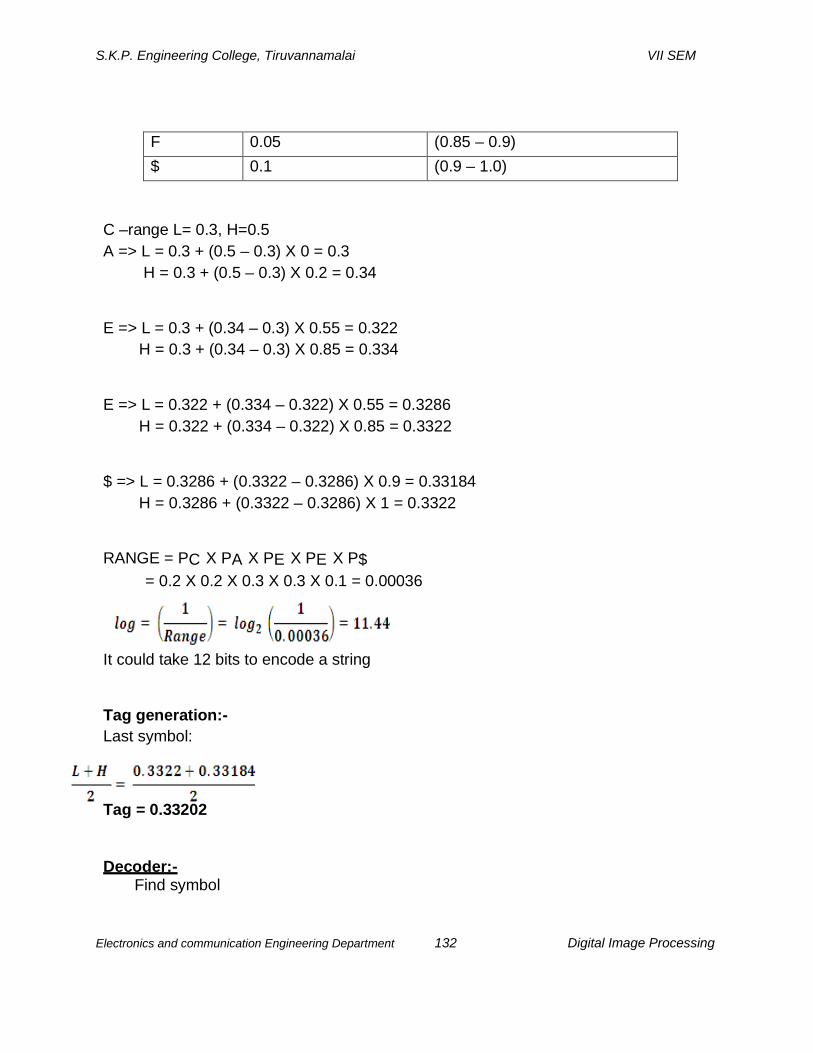
S.K.P. Engineering College, Tiruvannamalai VII SEM
Electronics and communication Engineering Department 132 Digital Image Processing
F 0.05 (0.85 – 0.9) $ 0.1 (0.9 – 1.0)
C –range L= 0.3, H=0.5 A => L = 0.3 + (0.5 – 0.3) X 0 = 0.3
H = 0.3 + (0.5 – 0.3) X 0.2 = 0.34 E => L = 0.3 + (0.34 – 0.3) X 0.55 = 0.322
H = 0.3 + (0.34 – 0.3) X 0.85 = 0.334 E => L = 0.322 + (0.334 – 0.322) X 0.55 = 0.3286
H = 0.322 + (0.334 – 0.322) X 0.85 = 0.3322 $ => L = 0.3286 + (0.3322 – 0.3286) X 0.9 = 0.33184
H = 0.3286 + (0.3322 – 0.3286) X 1 = 0.3322 RANGE = PC X PA X PE X PE X P$
= 0.2 X 0.2 X 0.3 X 0.3 X 0.1 = 0.00036
It could take 12 bits to encode a string
Tag generation:- Last symbol:
Tag = 0.33202
Decoder:-
Find symbol

S.K.P. Engineering College, Tiruvannamalai VII SEM
Electronics and communication Engineering Department 133 Digital Image Processing
Range – Low (s) < = value < range – high (S); Output (S);
Low = range – low (S);
High = range – high (S); Range = high – low; Value = (value - low) / Range;
}
Value output symbol low high Range 0.33202 C 0.3 0.5 0.2 0.1601 A 0.0 0.2 0.2 0.8005 E 0.55 0.85 0.3 0.8350 E 0.55 0.85 0.3 0.9500 $ 0.9 1.0 0.1
Value = (Tag value - low) / Range
= (0.33202 – 0.3) / 0.2 0.1601
Advantages of arithmetic coding:-
It achieves better performance then Huffman coding because the former treats the entire sequence of symbols as one unit. But the Huffman has the restriction of assigning an integral number of bits to each symbol.
Procedure:- 1) Encoder divides the numeric range from 0 to 1 into n number of segments. Where n is the number of different characters present in the message. 2) Determine the width of each segment which is equal to the probability of the related character. 3) Divide the segment of the first character in the string into n number of smaller segments.

S.K.P. Engineering College, Tiruvannamalai VII SEM
Electronics and communication Engineering Department 134 Digital Image Processing
Width of smaller segment = Base of segment + Range * low probability Range
Repeat the procedure until the termination of character.
Features: This coding statisfies noiseless coding thorem. An interval between 0 and 1 is defined by the code words for each sequence of source symbols. Arithmetic coding can treat the whole message as one unit. In practice, the input data is usually broken up into chunks to avoid error propagation.
Limitations: There are two practical factors affect the performance efficiency. i)The addition of the end –of –message indicator which is required to separate two messages. ii) The use of finite precision arithmetic. This problem can be handled by scaling strategy and rounding strategy.
6. Explain variable length coding with Huffman coding with one example.[April 2010] (or) Design a Huffman code for the source of a set character, A = { a1, a2, a3, a4, a5 } with the probabilities P = {0.2, 0.4, 0.2, 0.1, 0.1} Find Huffman code and calculate the average length of the code and redundancy[CO1-L1-May/June 2013]
Variable length coding:
It is the simplest lossless compression approach to reduce coding redundancy that is present in any natural binary coding of gray levels. This method assigns shortest possible code words to the most probable gray levels and longest code words to the least probable gray levels.
Types: Huffman code, arithmetic code
1. To order the probabilities of the given symbols in descending order 2. Next, source reduction is created by adding the lowest bottom two probability into a single symbol. This symbol is called as compound symbol which is replaced in next stage (they ordered in the descending order) 3. In this step each reduced source is coded.it starts from the smallest source

S.K.P. Engineering College, Tiruvannamalai VII SEM
Electronics and communication Engineering Department 135 Digital Image Processing
obtained from the previous step and goes back to the original source.
Step 1 and 2 repeated until a source with only two symbols is obtained.
Given data: A = {a1, a2, a3, a4, a5 } Probability P(a1 ) = 0.2, P(a2) = 0.4, P(a3) = 0.2, P(a4) = 0.1, P(a5) = 0.1
Letter Probability code word codeword length a2 0.4 00 2 a1 0.2 10 2 a3 0.2 11 2 a4 0.1 010 3 a5 0.1 011 3
Entropy:
In Huffman coding, each source symbol is mapped into a fixed sequence of code symbols. Also ,each symbol can be instantaneously decoded without referring the succeeding symbols in only one unique way.
The string of code symbols: 010 10 11 00 a4 a1 a3 a2
Advantages:
It provides the smallest number of code symbols per source symbol. It creates optimal code for set of symbols.

S.K.P. Engineering College, Tiruvannamalai VII SEM
Electronics and communication Engineering Department 136 Digital Image Processing
Coding/decoding is simple.
Disadvantages: It has the limitation that only one symbol can be coded at a time. Therefore, this coding is difficult when large number of symbols is to be coded. For J source symbols, it requires J-2 source reductions and J-2 code assignments. therefore computational complexity is more.
7. A source emits three symbols A, B, C with probabilities {0.5, 0.25, 0.25}respectively.construct an arithmetic code to encode the word ‘C A B’ [CO1-H1-Nov/Dec 2015]
Symbol probability range A 0.5 (0 - 0.5) B 0.25 (0.5– 0.75) C 0.25 (0.75 – 1)
C –range L= 0.75 ,H=1 A => L = 0.75 + (1 – 0.75) X 0 = 0.75
H = 0.75 + (1 – 0.75) X 0.5 = 0.875 B => L = 0.75 + (0.875 – 0.75) X 0.5 = 0.8125
H = 0.75 + (0.875 – 0.75) X 0.75 = 0.84375

S.K.P. Engineering College, Tiruvannamalai VII SEM
Electronics and communication Engineering Department 137 Digital Image Processing
The code word ‘CAB’can be assigned value between 0.8125-0.84375
8. What is the need for data compression? [CO1-L1-May/June 2014]
It is a process of reducing an amount of data required to represent the given quantity of information. Need for compression: Easy of processing and storage. To reduce the transmission bandwidth needed To reduce the required storage capacity Thus ,to achieve siginificant improvements of data throughput. Types of image compression technique Image compression
Lossless compression lossy compression
Loss less compression:
It provides image without any loss in information. Lossy compression:-
It provides higher level of data reduction but does not give perfect reproduction. Example - video conferencing.
Data redundancy:-
Various amount of data used to give the same amount of information.

S.K.P. Engineering College, Tiruvannamalai VII SEM
Electronics and communication Engineering Department 138 Digital Image Processing
Data redundancy is given by
Case 1:
If n1 = n, Cratio = 1, Rdata = 0 No redundant data
Case 2:
If n1 >> n2 Cratio = ∞, Rdata = 1 High redundant data
Case 3:
If n1 << n2 Cratio = 0, Rdata = ∞ n2 contains more data then its original information.
9. Explain about image compression models. [CO1-L1] A compression system consists of two distinct structural blocks: an encoder and a decoder. An input image f(x, y) is fed into the encoder, which creates a set of symbols from the input data. After transmission over the channel, the encoded representation is fed to the decoder,where a reconstructed output image f^(x, y) is generated. In general, f^(x, y) may or may not be an exact replica of f(x, y). If it is, the system is error free or information preserving; if not, some level of distortion is present in the reconstructed image. Both the encoder and decoder consist of two relatively independent functions or subblocks. The encoder is made up of a source encoder, which removes input redundancies, and a channel encoder, which increases the noise immunity of the source encoder's output. As would be expected, the decoder includes a channel decoder followed by a source decoder. If the channel between the encoder and decoder is noise free (not prone to error), the channel encoder and decoder are omitted, and the general encoderand decoder become the source encoder and decoder, respectively.

S.K.P. Engineering College, Tiruvannamalai VII SEM
Electronics and communication Engineering Department 139 Digital Image Processing
The Source Encoder and Decoder: The source encoder is responsible for reducing or eliminating any coding, interpixel, or psychovisual redundancies in the input image. The specific application and associated fidelity requirements dictate the best encoding approach to use in any given situation. Normally, the approach can be modeled by a series of three independent operations. Each operation is designed to reduce one of the three redundancies. The figure shown below depicts the corresponding source decoder. In the first stage of the source encoding process, the mapper transforms the input data into a (usually nonvisual) format designed to reduce interpixel redundancies in the input image. This operation generally is reversible and may or may not reduce directly the amount of data required to represent the image.

S.K.P. Engineering College, Tiruvannamalai VII SEM
Electronics and communication Engineering Department 140 Digital Image Processing
Run-length coding is an example of a mapping that directly results in data compression in this initial stage of the overall source encoding process. The representation of an image by a set of transform coefficients is an example of the opposite case. Here, the mapper transforms the image into an array of coefficients, making its interpixel redundancies more accessible for compression in later stages of the encoding process. The second stage, or quantizer block in Fig. (a), reduces the accuracy of the mapper's output in accordance with some preestablished fidelity criterion. This stage reduces the psychovisual redundancies of the input image. This operation is irreversible. Thus it must be omitted when error-free compression is desired. In the third and final stage of the source encoding process, the symbol coder creates a fixed- or variable-length code to represent the quantizer output and maps the output in accordance with the code. The term symbol coder distinguishes this coding operation from the overall source encoding process. In most cases, a variable-length code is used to represent the mapped and quantized data set. It assigns the shortest code words to the most frequently occurring output values and thus reduces coding redundancy. The operation, of course, is reversible. Upon completion of the symbol coding step, the input image has been processed to remove each of the three redundancies. 10. Explain lossless or Error-free compression. [CO1-L1]
LOSSLESS (OR) ERROR-FREE COMPRESSION • Error-free compression is the acceptable data reduction method since there is no loss of data •This lossless method is applicable to both binary and gray-scale images. • It provides compression ratios ranging from 2 to 10
Operations: All the lossless compression techniques are formed by two basic independent operations. They are: (i) Forming an alternative representation for the given image by which its interpixel
redundancies are reduced. (ii) Coding the representation to remove its coding redundancies.
Applications: Some important applications of lossless compression include the following: (i) Digital radiography

S.K.P. Engineering College, Tiruvannamalai VII SEM
Electronics and communication Engineering Department 141 Digital Image Processing
(ii) Processing of satellite imagery (iii) Archival of medical or business documents. Methods:
Four important methods to achieve lossless or error - free compression are:
Variable-Length Coding — Reduce Coding Redundancies LZW Coding Bit-Plane Coding Lossless Predicitive Coding
8. Explain Bit-Plane coding. [CO1-L1] BIT — PLANE CODING: Bit — plane coding is another method to reduce "interpixel redundancies" present in an image. • It works on the bit planes of an image individually.It can be applied to both monochrome and color images. This technique decomposes a multilevel image into a series of binary images or bit planes. Then, each binary image is compressed using any one binary compression method. Thus, it has 2 steps: (1) Bit plane decomposition (2) Compression of bit - planes
In gray code representation successive code words differ in only one bit position. These changes have very less effect on the m bit planes. Thus the effect due to small gray - level variations is reduced.
Example: The gray codes of 127 and 128 are 11000000 and 01000000. If they are adjacent gray levels, only the 7th bit plane will have a 0 to 1 transition.
Compression of Bit Planes: In order to reduce interpixel redundancies, a binary image or bit plane can be compressed using four coding techniques, known as (1) Constant Area Coding CAC) (2) One-Dimensional Run-Length Coding

S.K.P. Engineering College, Tiruvannamalai VII SEM
Electronics and communication Engineering Department 142 Digital Image Processing
(3) Two-Dimensional Run-Length Coding (4) Contour Tracing And Coding
(1) Constant Area Coding (CAC):
• This is a simple and effective method for bit plane compression.As its name states, It identifies large areas of contiguous i.e. neighboring l's or 0's using some special code words.
Procedure Generating the CAC requires the following three steps.
(i) Divide the image into blocks of size pxq pixels. (ii) Classify the blocks as all white, all black or mixed intensity
according to their gray levels. (iii) Assign the 1-bit code word '0' to the most probable or frequently
occurring category and assign the 2-bit codes 10 and 11 to the other two categories.
Since the bits representing constant gray level areas are replaced by a 1-bit or 2-bit code word, this method results in compression. White Block Skipping (WBS): • This is the method used when text documents with white dominant areas are compressed. • As the white areas are dominant, the few black regions present are combined with the mixed intensity areas. • Thus it assigns the 1-bit code word '0' to the highly probable solid white areas or blocks. • For all other blocks, a code with a 1 followed by the bit pattern of the block is used. Modified WBS The white block skipping method can be modified in two ways to make the compression more efficient. They are (1) In the first way, the solid white lines are coded as 0's and all other lines are coded with a '1' followed by the normal WBS code sequence.

S.K.P. Engineering College, Tiruvannamalai VII SEM
Electronics and communication Engineering Department 143 Digital Image Processing
(2) The second way is an iterative approach in which the solid white blocks are coded '0'. All other blocks are divided into smaller and smaller subblocks and similarly coded with a prefix code '1' followed by the block bit pattern. 4)Contour Tracing and Coding [Contour outline of an area]
Direct contour tracing is a method which represents a contour by two ways.They are (i)Using a set of boundary points (ii)Using a single boundary point and a set of directionals.
Predictive Differential quantizing (PDQ):PDQ is a scan-line-oriented contour tracing procedure. It shows clearly the important characteristics of relative address coding (RAC)and direct contour tracing techniques. The parameters of PDQ are illustrated in fig.
(1) ∆’-It is the difference between the starting coordinates of the front contours on adjacent lines. (2) ∆’’ - It is the difference between front-to-back contour lengths. (∆’, ∆’’) pair is generated by tracing the front and back contours of each object present in an image simultaneously. (3) New start message — This indicates the starting of new contours. (4) Merge message -This indicates the ending of old contours.
Double Delta Coding (DDC):
If the parameter ∆" in the PDQ technique is replaced by another parameter ∆'", the approach is called 'double delta coding' (DDC). Here, ∆"' is the difference between the back contour coordinates of adjacent lines.
Role of New Start and Merge Messages New start and merge are the special messages representing an object in addition to ∆' and ∆".
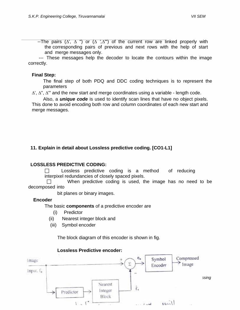
S.K.P. Engineering College, Tiruvannamalai VII SEM
Electronics and communication Engineering Department 144 Digital Image Processing
--The pairs (∆', ∆ ") or (∆ ',∆"') of the current row are linked properly with the corresponding pairs of previous and next rows with the help of start and merge messages only.
--- These messages help the decoder to locate the contours within the image correctly.
Final Step: The final step of both PDQ and DDC coding techniques is to represent the parameters
∆', ∆", ∆'" and the new start and merge coordinates using a variable - length code. Also, a unique code is used to identify scan lines that have no object pixels.
This done to avoid encoding both row and column coordinates of each new start and merge messages.
11. Explain in detail about Lossless predictive coding. [CO1-L1]
LOSSLESS PREDICTIVE CODING:
Lossless predictive coding is a method of reducing interpixel redundancies of closely spaced pixels.
When predictive coding is used, the image has no need to be decomposed into
bit planes or binary images. Encoder
The basic components of a predictive encoder are (i) Predictor
(ii) Nearest integer block and (iii) Symbol encoder
The block diagram of this encoder is shown in fig. Lossless Predictive encoder:

S.K.P. Engineering College, Tiruvannamalai VII SEM
Electronics and communication Engineering Department 145 Digital Image Processing
Encoding Process:
The process being taken place in the encoder is (1)First, each pixel of the input image, fn is loaded into the encoder one by one. (2)The predicator produces the anticipated value i.e. predicted value of the input pixel based on some past inputs. (3)Then,the output of the predictor is rounded to the nearest integer. The rounded value is denoted as f^n. (4)Now, the prediction error is obtained by the difference en = fn – f^n (5)The difference obtained is coded by the symbol encoder using a variable -length code. (6)The output of the symbol encoder gives the next element of the compressed data stream.
Decoder
The components of the predictive decoder are: (i) Symbol decoder (ii) Predictor The block diagram of this decoder is shown in fig.
Fig.Lossless predictive decoder

S.K.P. Engineering College, Tiruvannamalai VII SEM
Electronics and communication Engineering Department 146 Digital Image Processing
Decoding Process: The decoder performs the inverse operation of encoder. It receives the
variable -length code words from the encoder output and reconstructs the prediction error, en.
The operation of the decoder can be expressed as
fn =en+f^n Where f^n -Prediction of fn.
Role of Prediction Error:
Most of the interpixel redundancy is removed by the prediction and differencing process given in eqn.(1).
Mapping the input image into the prediction error causes entropy reduction.
This entropy reduction has a direct impact on the amount of compression. Thus, the extent of compression achieved depends on the prediction error.
Therefore, the probability density function (PDF) of the prediction error has a high peak at zero and characterized by small variance.
Advantages: Use of the lossless predictive coding has two advantages:
(i ) Large amount of interpixel redundancies can be reduced (i i ) Unlike other methods, the input images need no bit plane decomposition.
12.Explain wavelet coding system. Wavelet coding technique is based on the discrete wavelet transform.
Wavelet Transform: Wavelet Transform decomposes an image into a set of basis functions called wavelets. These basis functions are limited in duration. Therefore wavelet transforms are inherently local.The coefficients of wavelets represent the correlation between the wavelets and an image area. The concept behind wavelet coding is that the coefficients of a transform that decorrelates the pixels of an image can be coded more efficiently than the original pixels. Also, if most of the important visual information is packed i.e. confined into a small number of coefficients by the basis functions i.e. wavelets, the other

S.K.P. Engineering College, Tiruvannamalai VII SEM
Electronics and communication Engineering Department 147 Digital Image Processing
coefficients can be quantized or set to zero. This will produce only a little image distortion.
Wavelet Coding System: A wavelet coding system consists of an encoder and a decoder coding.The block diagram of a wavelet encoder is shown in fig.
Wavelet Encoder: The following steps are needed to encode a 2j x2j sized image (1) Select an analyzing wavelet, ψ and a minimum decomposition level,J-P. (2) Compute the discrete wavelet transform (DWT) of the image using the selected parameters. (3) If the wavelet has a complimentary scaling function φ, the fast wavelet transform (FWT) can be computed. (4) The output of the computed transform is horizontal. vertical and diagonal coefficients of the image with zero mean and Laplacian like distributions. (5) Now, the computed coefficients are quantized. Because many of these coefficients carry very less visual information, quantization helps to reduce(i) Intercoefficient redundancy and Coding redundancy (6)Atlast any one or more of the lossless coding techniques can be used of the symbol coding.
These techniques include: • Huffman coding
Arithmetic coding Bit-plane coding and Run-length coding
The block diagram of the decoder used for wavelet coding is shown in fig. This

S.K.P. Engineering College, Tiruvannamalai VII SEM
Electronics and communication Engineering Department 148 Digital Image Processing
decoder just inverts the opertions of the encoder. The only difference is that there is no quantization step. Because it is not possible to reverse the quantization exactly.
Advantage over Transform Coding: Wavelet transforms are both computationally efficient and inherently local. Therefore, unlike transform coding, wavelet coding does not need the original image to be subdivided. This removal of subdivision step eliminates the blocking artifact which characterizes DCT - based approximations at High compression ratios.
Influencing Factors: There are three major factors that affect three parameters of the wavelet coding system. The parameters affected are
Coding complexity Performance and Reconstruction error
The factors should be taken care are (1) Wavelet selection (2) Decomposition level selection (3) Quantizer design Wavelet Selection: The wavelets should be selected in such a way that they should have good ability to pack i.e. confine information into a small number of transform coefficients. Because, only is ability decides the extend i.e. depth of compression and reconstruction performance.
Selection Methods: Here, the wavelets are selected on the basis of forward and inverse transforms used for coding. But, they affect
(i) Computational complexity of the transforms and (ii) System's ability to compress and reconstruct images with acceptable error.
Thus, this method of selecting wavelets has an impact on all the aspects of wavelet coding system design and performance.

S.K.P. Engineering College, Tiruvannamalai VII SEM
Electronics and communication Engineering Department 149 Digital Image Processing
This method selects a transforming wavelet with a companion scaling function. Now,the transformation can be implemented as a sequence of digital filtering operations, where,Number of taps = Number of non zero wavelet and scaling vector coefficients.
Preferred Functions: The expansion functions i.e wavelets which are mostly used for wavelet - based compression are • Daubechies wavelets • Biorthogonal wavelets
Decomposition Level Selection The number of decomposition or transform levels is another important factor which affects Computational complexity of wavelet coding and Reconstruction error.When the number of decomposition levels increases,the number of operations required for the omputation of the forward and inverse transform also increases. This happens because a P-scale fast wavelet transform needs P filter bank iterations.Also, more decomposition levels produce large number of lower-scale coefficients. This affects the reconstructed image badly.
Selection Method: Due to the above reasons, in many applications. the number of transform levels is selected on the basis of resolution of the stored or transmitted images and scale of the lowest useful approximations.
Coefficient quantization is the largest factor which affects the wavelet coding compression and reconstruction error. Therefore, the quantizer used for encoding should be designed with care.
To Improve Quantization Effectiveness: Most of the quantizers used are uniform themselves. But still, the effectiveness of the quantization can be improved by two ways: (i) Introducing an enlarged quantization interval around zero, called the dead zone. (ii) Apadting i.e. varying the size of the quantization interval from scale to scale. These quantization intervals can be either found manually or computed automatically based on the image being compressed.

S.K.P. Engineering College, Tiruvannamalai VII SEM
Electronics and communication Engineering Department 150 Digital Image Processing
13. Explain about lossy predictive coding[CO1-L1]
Lossy Predictive Coding: In this type of coding, we add a quantizer to the lossless predictive model and examine the resulting trade-off between reconstruction accuracy and compression performance. As the following figure shows, the quantizer, which absorbs the nearest integer function of the error-free encoder, is inserted between the symbol encoder and the point at which the prediction error is formed. It maps the prediction error into a limited range of outputs, denoted e^n which establish the amount of compression and distortion associated with lossy predictive coding.
In order to accommodate the insertion of the quantization step, the error-free encoder of figure must be altered so that the predictions generated by the encoder and decoder are equivalent. As shown in fig, this is accomplished by placing the lossy encoder's predictor within a feedback loop, where its input, denoted f˙n, is generated as a function of past predictions and the corresponding quantized errors. the optimization criterion is chosen to minimize the mean-square prediction error, the quantization error is assumed to be negligible (e˙n ≈ en), and the prediction is constrained to a linear combination of m previous pixels. These restrictions are not essential, but they simplify

S.K.P. Engineering College, Tiruvannamalai VII SEM
Electronics and communication Engineering Department 151 Digital Image Processing
the analysis considerably and, at the same time, decrease the computational complexity of the predictor. The resulting predictive coding approach is referred to as differential pulse code modulation (DPCM).

S.K.P. Engineering College, Tiruvannamalai VII SEM
Electronics and communication Engineering Department 152 Digital Image Processing
Unit V
Image Representation And Recognition
Part-A
1. Specify the various image representation approaches. [CO1-L1] Chain codes, Polygonal approximation, Boundary segments
2. Define chain code. [CO1-L1] Chain codes are used to represent a boundary by a connected sequence of straight line segment of specified length and direction. Typically this representation is based on 4 or 8 connectivity of segments. The direction of each segment is coded by using a numbering scheme.
3. What are the demerits of chain code? [CO1-L1] The demerits of chain code are, i.The resulting chain code tends to be quite long. ii.Any small disturbance along the boundary due to noise cause changes in the code that may not be related to the shape of the boundary. 4. What is polygonal approximation method? [CO1-L1] Polygonal approximation is a image representation approach in which a digital boundary can be approximated with arbitrary accuracy by a polygon. For a closed curve the approximation is exact when the number of segments in polygon is equal to the number of points in the boundary so that each pair of adjacent points defines a segment in the polygon. 5. Specify the various polygonal approximation methods. [CO1-L1] The various polygonal approximation methods are i.Minimum perimeter polygons. ii.Merging techniques. iii.Splitting techniques. 6. Name few boundary descriptors. [CO1-L1] i.Simple descriptors. ii.Shape descriptors. iii.Fourier descriptors. 7. Define length of a boundary. [CO1-L1] The length of a boundary is the number of pixels along a boundary. Example, for a chain coded curve with unit spacing in both directions, the number of vertical and

S.K.P. Engineering College, Tiruvannamalai VII SEM
Electronics and communication Engineering Department 153 Digital Image Processing
horizontal components plus √2 times the number of diagonal components gives its exact length. 8. Give the formula for diameter of boundary[CO1-L1] The diameter of a boundary B is defined as Diam(B)=max[D(pi,pj)] i,j D-distance measure pi,pj-points on the boundary 9. Define eccentricity and curvature of boundary[CO1-L1] Eccentricity of boundary is the ratio of the major axis to minor axis. Curvature is the rate of change of slope. 10. Define shape numbers. [CO1-L1] Shape number is defined as the first difference of smallest magnitude. The order n of a shape number is the number of digits in its representation. 11. Give the Fourier descriptors for the following transformations[CO1-L1] (1)Identity (2) Rotation (3) Translation (4) Scaling (5) Starting point 12. Specify the types of regional descriptors[CO1-L1] Simple descriptors, Texture 13.Name few measures used as simple descriptors in region descriptors. [CO1-L1] i.Area ii.Perimeter. iii.Mean and median gray levels iv.Minimum and maximum of gray levels. v.Number of pixels with values above and below mean. 14. Define texture. [CO1-L1] Texture is one of the regional descriptors. It provides measure measures of properties such as smoothness, coarseness and regularity. 15. Define compactness. [CO1-L1] Compactness of a region is defined as (perimeter)2 / area. It is a dimensionless quantity and is insensitive to uniform scale changes. 16. List the approaches to describe texture of a region. [CO1-L1] The approaches to describe the texture of a region are, i.Statistical approach. ii.Structural approach. iii.Spectural approach. 17.What is thinning or skeletonizing algorithm? [CO1-L1]

S.K.P. Engineering College, Tiruvannamalai VII SEM
Electronics and communication Engineering Department 154 Digital Image Processing
An important approach to represent the structural shape of a plane region is to reduce it to a graph. This reduction may be accomplished by obtaining the skeletonizing algorithm. It plays a central role in a broad range of problems in image processing, ranging from automated inspection of printed circuit boards to counting of asbestos fibers in air filter. 18. What is pattern and pattern class? [CO1-L1] Pattern is a quantitative or structural description of an object or some other entity of interest in an image. It is formed by one or more descriptors. Pattern class is a family of patterns that share some common properties. Pattern classes are denoted as w1 w2 w3 ……… wM , where M is the number of classes.
19. What is pattern recognition? [CO1-L1] It involves the techniques for arranging pattern to their respective classes by automatically and with a little human intervention. 20. What are the three principle pattern arrangements? [CO1-L1] The three principal pattern arrangements are vectors, Strings and trees. Pattern vectors are represented by old lowercase letters such as x ,y, z and it is represented in the form x=[x1, x2, ……….., xn ]. Each component x represents I th descriptor and n is the number of such descriptor.
21.What is meant by markers? [CO1-L1] An approach used to control over segmentation is based on markers. marker is a connected component belonging to an image. We have internal markers, associated with objects of interest and external markers associated with background. 22. What are the 2 principles steps involved in marker selection? [CO1-L1] The two steps are 1. Preprocessing2. Definition of a set of criteria that markers must satisfy. 23.Describe statistical approach[CO1-L1] Statistical approaches describe smooth,coarse,grainy characteristics of texture.This is the simplest one compared to others. It describes texture using statistical moments of the gray-level histogram of an image or region. 24. Define gray-level co-occurrence matrix. [CO1-L1] A matrix C is formed by dividing every element of A by n(A is a k x k matrix and n is the total number of point pairs in the image satisfying P(position operator). The matrix C is called gray-level cooccurrence matrix if C depends on P, the presence of given texture patterns may be detected by choosing an appropriate position operator.

S.K.P. Engineering College, Tiruvannamalai VII SEM
Electronics and communication Engineering Department 155 Digital Image Processing
25. Explain structural and spectral approach. [CO1-L1] Structural approach deals with the arrangement of image primitives such as description of texturebased on regularly spaced parallel lines.Spectral approach is based on properties of the Fourier spectrum and primarily to detect global periodicity in an image by identifying high energy, narrow peaks in spectrum. There are 3 features of Fourier spectrum that are useful for texture description. They are i) Prominent peaks in spectrum gives the principal direction of texture patterns. ii) The location of peaks in frequency plane gives fundamental spatial period of patterns.iii) Eliminating any periodic components by our filtering leaves non- periodic image elements
PART-B
1.Explain the boundary representation of object and chain codes. [CO1-L1]
BOUNDARY REPRESENTATION: Boundary representation represents a region in terms of its external characteristics.Therefore,it is also known as ‘external representation’. Some of the important approaches of boundary representation are: (1) Chain codes (2) Polygonal approximations (3) Boundary segments (4) Signatures and (5) Skeletons Chain codes: Chain codes represents a boundary by using a connected sequence of straight-line segments with specified length and direction. This representation is based on two types of connectivity of the segments ,known as 4-Connectivity and 8-Connectivity . Direction Numbers: The direction of each segment in the chain codes is given a number.The numbering scheme used for this coding is shown in fig.

S.K.P. Engineering College, Tiruvannamalai VII SEM
Electronics and communication Engineering Department 156 Digital Image Processing
Fig.5.1 figure number representation
Procedure: A grid format with equal spacing in the x- and y- directions is used to process digital images. using this grid a chain code can be created by following a boundary in clockwise direction. Then, each segment connecting a pair of pixels is assigned a direction. This method is not accepted. Because (1)The resulting chain of codes is very long (2)Noise or imperfect segmentation may produce small disturbances in the boundary. This creates changes in the code which is not desired.
Resampling: The above two drawbacks in the normal procedure can be overcome by the process of sampling. This process has the following steps. (1) first, the boundary is resampled by selecting a larger grid spcing as shown in fig. (2)Then, the boundary is traversed i.e, tracked and at the same time, boundary points are assigned to each node of the large grid. this assignment depends on the proximity i.e, nearness of the original boundary to the nodes as shown in fig.
Fig.5.2 Resampling method

S.K.P. Engineering College, Tiruvannamalai VII SEM
Electronics and communication Engineering Department 157 Digital Image Processing
Chain code Generation: Now, to represent the resampled boundary, two types of codes can be generated, which are (1) 4- directional chain code (2) 8- directional chain code The shortest allowable 4-path or the 4 - code is shown in fig. Its starting point is at the top,left corner and the chain code obtained is 0033………………1101 Similarly, the shortest allowable 8-path or the 8-code is shown in fig. Whose starting point is at the top, left corner and the chain code obtained is
0766…………………………1212
Fig 5.3 .chain code representation
The chain codes should be normalized with respect to its starting point,since it depends on the starting point.
2. Explain Polygonal approximations. [CO1-L1] The goal of the polygonal approximation is to capture the ‘essence’ of the boundary shape with the fewest possible number of polygonal segments. This approximation is perfect when each pair of adjacent points in the boundary is assigned to a segment in the polygon.

S.K.P. Engineering College, Tiruvannamalai VII SEM
Electronics and communication Engineering Department 158 Digital Image Processing
=>Number of segments in the polygon = number of points in the boundary.
Types: Three important types of polygonal approximations are available. These methods are preferred for many image processing applications. They are ; (1) Minimum perimeter polygons (2) Merging techniques (3) Splitting techniques (1) Minimum perimeter polygons [Perimeter -> The outer boundary] This method approximates a digital boundary with a minimum perimeter polygon. Procedure: The steps followed in this method are explained with an example below.Consider the boundary as shown in fig; (1) First,enclose the boundary using a sampling grid having a set of concatenated cells as shown in fig.These cells show the inside and outside walls of the boundary. (2) Assume the boundary as a rubber band which is placed in between the two walls. (3) Now,imagine that the rubber band is shirnked so that it touches the inside walls i.e, cell strips. The shape taken after shrinking gives the minimum perimeter polygon shown in fig. This kind of approximation is known as ‘rubber – band approximation’.
Fig.5.4 rubber – band approximation
(2) Merging Techniques Polygonal approximation problem can be handled by merging techniques also.These techniques may be based on some criteria such as average error. Procedure:

S.K.P. Engineering College, Tiruvannamalai VII SEM
Electronics and communication Engineering Department 159 Digital Image Processing
One of the important merging techniques is explained below; (1)Set a threshold for least square error (2)Merge some points along the boundary. This is done until the least square error line fit of the points merged so far exceeds the threshold. (3)When it exceeds, store the parameters of the line and set the error to 0. (4)Repeat the steps (2) and (3) by merging new points until the error again exceeds the threshold. Thus many lines are created around the boundary. (5) At last, the intersection produced by adjacent line segments give the vertices i.e, corner points of the polygon, and joining the vertices will form the polygon.
Drawback: The vertices resulting from this method are not exactly related with inflections such as corners because a new line is started only after the error threshold is exceeded.
Splitting a boundary into segments:
Thus, the obtained vertices are A,C,B and E. Joining these vertices results in the polygon which represents the given boundary. It is illustrated in fig.

S.K.P. Engineering College, Tiruvannamalai VII SEM
Electronics and communication Engineering Department 160 Digital Image Processing
Advantage: The advantage of this splitting technique is that it searches for prominent i.e, visible inflection points such as corners and thus the resulting vertices produce a good polygon approximation for the boundary.
3. Write short notes on Signatures. [CO1-L1] Signatures: A signature is a 1-D functional representation of a boundary. It is used to reduce the original 2-D boundary to a 1-D function so that the description becomes easier. The basic idea of this method is to (i) Remove the dependency on size and (ii) Preserve the shape Distance-Versus – Angle Signature: There are many ways to generate a signature. One way is to plot the distance from centroid to the boundary as a function of angle. An example is shown in fig.5.25.it is called as’ distance-versus-angle’ signature.
Fig,5.7 Distance-versus-angle signatures:

S.K.P. Engineering College, Tiruvannamalai VII SEM
Electronics and communication Engineering Department 161 Digital Image Processing
4. Explain Boundary Segments. [CO1-L1] Boundary Segments This is a type of boundary representation in which a boundary is decomposed into segments. It is used when the boundary has one or more concavities i.e, curves that carry shape information.The decomposition procedure is used to (i)Reduce the complexity of the boundary and (ii) simplify the description process Convex Hull, H: A set ‘A’ is said to be convex if the straight line joining any two points in ‘A’ lies entirely within ‘A’. The convex hull, H of an arbitrary set ‘S’ is the smallest convex set containing S. The set difference H- S is called the convex deficiency of S. The convex hull of the region enclosed by the boundary is used as a tool for efficient decomposition of the boundary. Procedure: Consider the boundary of an object ‘S’ shown in fig a. (1) First, the convex deficiency of the set i.e, object S is defined, which is the shaded region in the fig b (2)Next, the contour i.e, outline of S is followed and the points at which there is a transition into or out of the convex deficiency are marked. (3)These points are the partitioning points that give the segmented boundary. The result obtained is shown in fig.
Fig 5.7 (a) representation of boundary segments

S.K.P. Engineering College, Tiruvannamalai VII SEM
Electronics and communication Engineering Department 162 Digital Image Processing
Advantages: The advantage of segmenting a boundary using convex deficiency is that it is independent of the size and orientation of the given region. The convex hull and its deficiency can also be used for describing a region and its boundary. Drawback: Factors like digitalization, noise and variations in segmentation may lead to irregular boundaries of regions. Such boundaries produce convex deficiencies with small, meaningless components scattered randomly throughtout the boundary. This results in an inefficient decomposition processs.
5. Explain in detail the various Boundary descriptors with a neat diagram. [CO1-L1] Boundary descriptors describe the boundary of a region using the features of the boundary. Two important type of boundary descriptors are (1) Simple descriptors (2) Fourier descriptors Some quantities which are used to describe the boundary of a region are (1)shape numbers and (2)Statistical moments
Simple Descriptors Some simple descriptors used to describe a boundary are explained below
(1)Length: The length of a boundary is one of the simplest descriptors.It is given by the number of pixels along a boundary. For a chain coded curve which has unit spacing in both directions,the length is obtained by, Length =(𝑁𝑁𝑢𝑢𝑚𝑚𝑏𝑏𝑒𝑒𝑟𝑟 𝑜𝑜𝑓𝑓 𝑣𝑣𝑒𝑒𝑟𝑟𝑡𝑡𝑖𝑖𝑐𝑐𝑎𝑎𝑙𝑙 𝑎𝑎𝑛𝑛𝑑𝑑𝐻𝐻𝑜𝑜𝑟𝑟𝑖𝑖𝑧𝑧𝑜𝑜𝑛𝑛𝑡𝑡𝑎𝑎𝑙𝑙 𝑐𝑐𝑜𝑜𝑚𝑚𝑝𝑝𝑜𝑜𝑛𝑛𝑒𝑒𝑛𝑛𝑡𝑡𝑠𝑠) + √2(𝑁𝑁𝑢𝑢𝑚𝑚𝑏𝑏𝑒𝑒𝑟𝑟 𝑜𝑜𝑓𝑓 𝑑𝑑𝑖𝑖𝑎𝑎𝑔𝑔𝑜𝑜𝑛𝑛𝑎𝑎𝑙𝑙𝑐𝑐𝑜𝑜𝑚𝑚𝑝𝑝𝑜𝑜𝑛𝑛𝑒𝑒𝑛𝑛𝑡𝑡𝑠𝑠)
(2) Diameter: This is another useful descriptor.The diameter of a boundary B is expressed as Diam(B) =max [ 𝐷𝐷(𝑝𝑝𝑖𝑖,𝑝𝑝𝑗𝑗)] Where,D-A distance measure pi,pj –Points on the boundary
(3)Major axis:

S.K.P. Engineering College, Tiruvannamalai VII SEM
Electronics and communication Engineering Department 163 Digital Image Processing
The major axis of a boundary is defined as the line segment connecting the two extreme points of its diameter. (4)Minor axis: The minor axis of a boundary is defined as the line perpendicular to the major axis. (5)Eccentricity The ratio of the major axis to the minor axis is called the eccentricity of a boundary. i.e, Eccentricity = 𝑀𝑀𝑎𝑎𝑗𝑗𝑜𝑜𝑟𝑟 𝑎𝑎𝑥𝑥𝑖𝑖𝑠𝑠𝑀𝑀𝑖𝑖𝑛𝑛𝑜𝑜𝑟𝑟 𝑎𝑎𝑥𝑥𝑖𝑖𝑠𝑠
(6) Basic Rectangle The major axis intersects with the boundary at two points and the minor axis also intersects with the boundary at two points.A box which completely enclose the boundary by passing through these four outer points is called the ‘basic rectangle’. (7)Curvature: Curvature of a boundary is defined as the rate of change of its slope.But,measuring the curvature of a point on a digital boundary is very difficult.Therefore,the different between the slope of a adjacent boundary segments can be used as the descriptor for the curvature at the point of intersection of the two segments. When the boundary is traversed in the clockwise direction, the following can be defined. If the change in slope at a vertex point p is positive,p is said to be part of a convex segment. (i) If the change in slope at p is negative,p is said to be part of a concave segment. (ii) If the change is less than 100,p is a part of a nearly straight segment (iii) If the change is greater than 900,p is corner point. 6. Explain in detail the various FOURIER descriptors with a necessary equations.
[CO1-L1] FOURIER DESCRIPTORS: Fourier descriptors describe a digital boundary by considering it as a complex sequence.This has the advantage that it reduces a 2-D problem to a 1-D problem. Consider the digital boundary shown in fig.,which has ‘K’ number of points in them xy-plane.

S.K.P. Engineering College, Tiruvannamalai VII SEM
Electronics and communication Engineering Department 164 Digital Image Processing
Fig.5.8 Fourier Descriptors Starting from a point (𝑥𝑥0,0) and following the boundary in anticlockwise direction,its coordinate pairs are: (𝑥𝑥0,0), (𝑥𝑥1,𝑦𝑦1), (𝑥𝑥2,𝑦𝑦2),……………. (𝑥𝑥𝑘𝑘−1,−1) The coordinates can be represented as, x(k) = 𝑥𝑥𝑘𝑘 and y(k) = 𝑦𝑦𝑘𝑘 -------------------------(1) Now, the sequence of coordinates of the boundary are s(k) = [x(k),y(k)],for k = 0,1,2,……………….K-1 --------------------------------(2) Also,each coordinate pair can be represented as a complex number in the form s(k) = x(k) + jy(k) for k = 0,1,2,……………….K-1 --------------------------(3) Where,x axis – considered as the real axis,y axis – considered as the imaginary axis. Fourier Descriptors: The forward discrete Fourier transform (DFT) of the complex sequence s(k) is expressed as a(u) = 1𝐾𝐾 Σ𝑠𝑠(𝑘𝑘)𝐾𝐾−1𝐾𝐾=0𝑒𝑒−𝑗𝑗2𝜋𝜋𝑢𝑢𝑘𝑘𝑘𝑘 for u= 0,1,2,…………….K-1------------------------(4) Here,the complex co-efficients,a(u) obtained are referred to as the ‘Fourier descriptors’ of the boundary. Restoration:

S.K.P. Engineering College, Tiruvannamalai VII SEM
Electronics and communication Engineering Department 165 Digital Image Processing
The sequence s(k) can be restored by taking the inverse Fourier transform of the Fourier descriptors given by s(k) = Σ𝑎𝑎(𝑢𝑢)𝐾𝐾−1𝑢𝑢=0𝑒𝑒𝑗𝑗2𝜋𝜋𝑢𝑢𝑘𝑘𝑘𝑘 for k= 0,1,2,…………….K-1 ---------------------------(5) To reduce the number of terms used for reconstruction ,only the first P coefficients can be selected rather than using all the Fourier co-efficients.This is obtaining by setting a(u) = 0 for u > P – 1 in eqn (5) the resulting approximation is s^(k) = Σ𝑎𝑎(𝑢𝑢)𝑃𝑃−1𝑢𝑢=0𝑒𝑒𝑗𝑗2𝜋𝜋𝑢𝑢𝑘𝑘𝑘𝑘 for k= 0,1,2,…………….K-1 ---------------------------(6) Here,when the number of selected coefficients,P decreases,the amount of boundary information loss increases. Basic Properties: (1)Rotation: It states that ‘multiplying a point by 𝑒𝑒𝑗𝑗𝜃𝜃,rotates the point by an angle 𝛉𝛉 about the origin in the complex plane’. Therefore, to rotate the sequence s(k) about the origin, all points in s(k) are multiplied by 𝑒𝑒𝑗𝑗𝜃𝜃. Rota te d s e que nce = s (k). 𝑒𝑒𝑗𝑗𝜃𝜃 The Fourier descriptors of the rotated sequence is, ar(u) = 1𝐾𝐾 Σ𝑠𝑠(𝑘𝑘)𝑒𝑒𝑗𝑗𝜃𝜃𝐾𝐾−1𝐾𝐾=0.𝑒𝑒−𝑗𝑗2𝜋𝜋𝑢𝑢𝑘𝑘𝑘𝑘 for u= 0,1,2,…………….K-1 ------------------------(7) =a(u). 𝑒𝑒𝑗𝑗𝜃𝜃 2. Translation: Translation adds a constant displacement to all coordinates in the boundary.It is obtained as (k) = s(k) + Δxy ----------------------------------(8) Where, Δxy = Δx + jΔy Only when u = 0,the translation affects the descriptors. 3. Starting Point: The starting point of a sequence can be changed from k =0 to k= k0 by using the expression, (k) = s(k- k0) 𝑠𝑠𝑝𝑝=(k- k0) + jy(k- k0) --------------------------------(9) 7. Explain in detail about Shape Numbers. [CO1-L1] The shape number of a boundary is defined as first difference of smallest magnitude. The order ‘n’ of a shape number is defined as the number of digits in its representation. Procedure: To find the shape number of order ‘n’ for a boundary,the steps required are:

S.K.P. Engineering College, Tiruvannamalai VII SEM
Electronics and communication Engineering Department 166 Digital Image Processing
(1)First,find the rectangle of order ‘n’ whose eccentricity is well suited for the basic rectangle. (2)Establish the grid size using this new rectangle. (3)Align chain-code directions for the resulting grid. (4)Obtain the chain code. (5)Find the first difference and use it to compute the shape number. A shape of order 4 is shown in fig.Starting from the top left corner,its shape number is obtained as given.
Fig.5.9 example for shape numbers 8. Explain Regional descriptors. [CO1-L1] Regional descriptors are used to describe image regions, that is regions enclosed by boundaries. In practice, regional descriptors are used with boundary descriptors. Some important regional descriptors are: (1)Simple descriptors (2)Texture (3)Topological descriptors (4)Moments of two-dimensional functions Simple Descriptors: The simple descriptors used to describe a region are given below: (1) Area: The area of a region is defined as the number of pixels in a region. This is one of the simplest regional descriptor (2)Perimeter: The perimeter of a region is defined as the length of its boundary. The perimeter and area used as descriptors when the size of a region is fixed (3)Compactness:

S.K.P. Engineering College, Tiruvannamalai VII SEM
Electronics and communication Engineering Department 167 Digital Image Processing
- The compactness of a region is defined as (perimeter)2/area. -Compactness is a dimensionless quantity and therefore it is not sensitive to uniform scale changes. - It is also insensitive to orientation and thus the error introduced by rotation of a digital region can be avoided. - Its value is minimum for disk — shaped regions. (4) Other Measures: Some other simple measures for describing a region are: (i)Mean and median of the gray levels (ii)Minimum and maximum gray-level values (iii)Number of pixels with values above and below the mean. 9. Briefly explain Topological descriptors. [CO1-L1] Topological Descriptors: Topology is defined as the study of properties of an image which are not affected by any deformation such as stretching, rotation etc. These properties will change only when there is tearing or joining i.e. folding of the image. Therefore, they are also called rubber — sheet distortions. Using such properties to describe an image or region is known as the topological description. Descriptors Used: Some of the topological descriptors used to describe a region are: • Number of holes in the region • Number of connected components of the region etc. Example: Consider the region shown in fig. Let its topological descriptor is defined by the number of holes in the region.

S.K.P. Engineering College, Tiruvannamalai VII SEM
Electronics and communication Engineering Department 168 Digital Image Processing
Fig.5.10 Example for topological descriptor This property will not be changed if the figure is stretched or rotated. It will be affected only if the region is torn or folded. Thus, some additional features are provided by the topological descriptors which are useful to characterize the regions. 10. Explain in detail about Patterns and Pattern Classes. [CO1-L1] Patterns and Pattern Classes:
A pattern is an arrangement of descriptors,.The name feature is used often in the pattern recognition literature to denote a descriptor. A pattern class is a family of patterns that share some common properties. Pattern classes are denoted ω1,ω2,………….,ωW,where W is the number of classes. Pattern recognition by machine involves techniques for assigning patterns to their respective classes—automatically and with as little human intervention as possible. Three common pattern arrangements used in practice are vectors (for quantitative descriptions) and strings and trees (for structural descriptions). Pattern vectors are represented by bold lowercase letters, such as x, y, and z, and take the form

S.K.P. Engineering College, Tiruvannamalai VII SEM
Electronics and communication Engineering Department 169 Digital Image Processing
where each component, xi, represents the ith descriptor and n is the total number of such descriptors associated with the pattern. Pattern vectors are represented as columns (that is, n x 1 matrices). Hence a pattern vector can be expressed in the form shown in Eqn. (1) or in the equivalent form x = (x1, x2, , xn)T, where T indicates transposition. The nature of the components of a pattern vector x depends on the approach used to describe the physical pattern itself. Let us illustrate with an example that is both simple and gives a sense of history in the area of classification of measurements. In our present terminology,each flower is described by two measurements,which leads to a 2-D pattern vector of the form
where x1 and x2 correspond to petal length and width, respectively. The three pattern classes in this case, denoted ω1, ω2, and ω3, correspond to the varieties setosa, virginica, and versicolor,respectively. Because the petals of flowers vary in width and length, the pattern vectors describing these flowers also will vary, not only between different classes, but also within a class.The above Figure shows length and width measurements for several samples of each type of iris. After a set of measurements has been selected (two in this case), the components of a pattern vector become the entire description of each physical sample. Thus each flower in this case becomes a point in 2-D Euclidean space.We note also that measurements of petal width and length in this case adequately separated the class of Iris setosa from the other two but did not separate as successfully the virginica and versicolor types from each other. This result illustrates the classic feature selection problem, in which the degree of class separability depends strongly on the choice of descriptors selected for an application. 11. Briefly explain about Matching. [CO1-L1] Recognition techniques based on matching represent each class by a prototype pattern vector. An unknown pattern is assigned to the class to which it is closest in terms of a predefined metric. The simplest approach is the minimum distance classifier, which, as its name implies, computes the (Euclidean) distance between the unknown and each of the prototype vectors. It chooses the smallest distance to make a decision. We also discuss an approach based on correlation,which can be formulated directly in terms of images and is quite intuitive.

S.K.P. Engineering College, Tiruvannamalai VII SEM
Electronics and communication Engineering Department 170 Digital Image Processing
Minimum distance classifier Suppose that we define the prototype of each pattern class to be the mean vector of the patterns of that class:
where NJ is the number of pattern vectors from class ωj and the summation is taken over these vectors. As before, W is the number of pattern classes. One way to determine the class membership of an unknown pattern vector x is to assign it to the class of its closest prototype, as noted previously. Using he Euclidean distance to determine closeness reduces the problem to to computing the distance measures. The decision boundary between classes ωi , and ωj for a minimum distance classifier is
The surface given by the above equation is is the perpendicular bisector of the line segment joining 𝑚𝑚𝑖𝑖 and 𝑚𝑚𝑗𝑗. For n = 2, the perpendicular bi-sector is a line, for n = 3 it is a plane, and for n > 3 it is called a hyperplane.The two classes, Iris versicolor and Iris setosa, denoted ω1 and ω2, respectively, have sample mean vectors m1 = (4.3, 1.3)T and m2 = (1.5, 0.3)T. The decision functions are

S.K.P. Engineering College, Tiruvannamalai VII SEM
Electronics and communication Engineering Department 171 Digital Image Processing
Fig.5.11 plot of this boundary The above figure shows a plot of this boundary (note that the axes are not to the same scale). Substitution of any pattern vector from class ω1 would yield d12(x) > 0. Conve rs e ly, a ny pa tte rn from cla s s ω2 would yie ld d12(x) < 0. In othe r words , give n an unknown pattern belonging to one of these two classes, the sign of d12(x) to one of these two classes, the sign of d12(x) would be sufficient to determine the pattern's class membership.