site-resolved imaging with the fermi gas microscope
TRANSCRIPT
Site-Resolved Imaging withthe Fermi Gas MicroscopeThe Harvard community has made this
article openly available. Please share howthis access benefits you. Your story matters
Citation Huber, Florian Gerhard. 2014. Site-Resolved Imaging with the FermiGas Microscope. Doctoral dissertation, Harvard University.
Citable link http://nrs.harvard.edu/urn-3:HUL.InstRepos:12274189
Terms of Use This article was downloaded from Harvard University’s DASHrepository, and is made available under the terms and conditionsapplicable to Other Posted Material, as set forth at http://nrs.harvard.edu/urn-3:HUL.InstRepos:dash.current.terms-of-use#LAA

Site-Resolved Imaging with the Fermi Gas Microscope
A dissertation presented
by
Florian Gerhard Huber
to
The Department of Physics
in partial fulfillment of the requirements
for the degree of
Doctor of Philosophy
in the subject of
Physics
Harvard University
Cambridge, Massachusetts
May 2014

c© 2014 Florian Gerhard Huber
All rights reserved.

Dissertation Advisor:Professor Markus Greiner
Author:Florian Gerhard Huber
Site-Resolved Imaging with the Fermi Gas Microscope
Abstract
The recent development of quantum gas microscopy for bosonic rubidium atoms trapped in
optical lattices has made it possible to study local structure and correlations in quantum
many-body systems. Quantum gas microscopes are a perfect platform to perform quantum
simulation of condensed matter systems, offering unprecedented control over both internal
and external degrees of freedom at a single-site level. In this thesis, this technique is
extended to fermionic particles, paving the way to fermionic quantum simulation, which
emulate electrons in real solids.
Our implementation uses lithium, the lightest atom amenable to laser cooling. The
absolute timescales of dynamics in optical lattices are inversely proportional to the mass.
Therefore, experiments are more than six times faster than for the only other fermionic
alkali atom, potassium, and more then fourteen times faster than an equivalent rubidium
experiment.
Scattering and collecting a sufficient number of photons with our high-resolution imaging
system requires continuous cooling of the atoms during the fluorescence imaging. The
lack of a resolved excited hyperfine structure on the D2 line of lithium prevents efficient
conventional sub-Doppler cooling. To address this challenge we have applied a Raman
sideband cooling scheme and achieved the first site-resolved imaging of ultracold fermions
in an optical lattice.
iii
Contents
Abstract . . . . . . . . . . . . . . . . . . . . . . . . . . . . . . . . . . . . . . . . . . . . iiiAcknowledgments . . . . . . . . . . . . . . . . . . . . . . . . . . . . . . . . . . . . . vi
Introduction 1Analog Quantum Simulation . . . . . . . . . . . . . . . . . . . . . . . . . . . . . . . 2Fermi Gas Microscopy . . . . . . . . . . . . . . . . . . . . . . . . . . . . . . . . . . . 3Why Lithium? . . . . . . . . . . . . . . . . . . . . . . . . . . . . . . . . . . . . . . . . 4Synopsis . . . . . . . . . . . . . . . . . . . . . . . . . . . . . . . . . . . . . . . . . . . 5
1 Theory 71.1 Atomic Physics . . . . . . . . . . . . . . . . . . . . . . . . . . . . . . . . . . . . 7
1.1.1 Magnetic Fields And Microwave Transitions . . . . . . . . . . . . . . . 71.1.2 Light-Matter Interaction . . . . . . . . . . . . . . . . . . . . . . . . . . . 10
1.2 Feshbach Resonances . . . . . . . . . . . . . . . . . . . . . . . . . . . . . . . . . 181.2.1 Feshbach Resonances In Reduced Dimensions . . . . . . . . . . . . . . 20
1.3 Quantum Harmonic Oscillator . . . . . . . . . . . . . . . . . . . . . . . . . . . 201.3.1 One-Dimensional Harmonic Oscillator . . . . . . . . . . . . . . . . . . 211.3.2 Ensembles In A Harmonic Oscillator . . . . . . . . . . . . . . . . . . . 22
1.4 Optical Potentials . . . . . . . . . . . . . . . . . . . . . . . . . . . . . . . . . . . 261.4.1 Gaussian Beams . . . . . . . . . . . . . . . . . . . . . . . . . . . . . . . 261.4.2 Travelling Wave Potentials . . . . . . . . . . . . . . . . . . . . . . . . . . 311.4.3 Standing Wave Potentials . . . . . . . . . . . . . . . . . . . . . . . . . . 331.4.4 Noise-Induced Heating . . . . . . . . . . . . . . . . . . . . . . . . . . . 38
1.5 Physics Of Optical Lattices . . . . . . . . . . . . . . . . . . . . . . . . . . . . . 401.5.1 Band Structure Calculation . . . . . . . . . . . . . . . . . . . . . . . . . 401.5.2 Tight Binding Model . . . . . . . . . . . . . . . . . . . . . . . . . . . . . 471.5.3 Bose-Hubbard Model . . . . . . . . . . . . . . . . . . . . . . . . . . . . 491.5.4 Fermi-Hubbard Model . . . . . . . . . . . . . . . . . . . . . . . . . . . . 51
2 Raman Cooling 552.1 Vibrational Transitions . . . . . . . . . . . . . . . . . . . . . . . . . . . . . . . . 55
iv

2.2 Raman Transitions . . . . . . . . . . . . . . . . . . . . . . . . . . . . . . . . . . 572.3 Optical Pumping: Coherent Vs. Incoherent Scattering . . . . . . . . . . . . . . 592.4 Raman Sideband Cooling In A Bias Field . . . . . . . . . . . . . . . . . . . . . 602.5 Three-Dimensional Cooling . . . . . . . . . . . . . . . . . . . . . . . . . . . . . 622.6 Alignment . . . . . . . . . . . . . . . . . . . . . . . . . . . . . . . . . . . . . . . 632.7 Raman Sideband Cooling At Zero Field . . . . . . . . . . . . . . . . . . . . . . 642.8 Heating Mechanisms . . . . . . . . . . . . . . . . . . . . . . . . . . . . . . . . . 652.9 Raman Imaging . . . . . . . . . . . . . . . . . . . . . . . . . . . . . . . . . . . . 67
2.9.1 Pulsed Raman Imaging . . . . . . . . . . . . . . . . . . . . . . . . . . . 682.9.2 Fidelity: Imaging A 3× 3 Plaquette Or Single Atom Minesweeper . . 702.9.3 Monte-Carlo Imaging Simulation . . . . . . . . . . . . . . . . . . . . . 73
3 Experimental Setup 753.1 Vacuum System . . . . . . . . . . . . . . . . . . . . . . . . . . . . . . . . . . . . 75
3.1.1 Main Chamber . . . . . . . . . . . . . . . . . . . . . . . . . . . . . . . . 773.1.2 Glass Cell . . . . . . . . . . . . . . . . . . . . . . . . . . . . . . . . . . . 77
3.2 Lasers . . . . . . . . . . . . . . . . . . . . . . . . . . . . . . . . . . . . . . . . . . 793.2.1 D2 Lasers . . . . . . . . . . . . . . . . . . . . . . . . . . . . . . . . . . . 793.2.2 D1 Laser And Raman Laser . . . . . . . . . . . . . . . . . . . . . . . . . 793.2.3 High Power ODT . . . . . . . . . . . . . . . . . . . . . . . . . . . . . . . 803.2.4 Dimple . . . . . . . . . . . . . . . . . . . . . . . . . . . . . . . . . . . . . 843.2.5 Lattice . . . . . . . . . . . . . . . . . . . . . . . . . . . . . . . . . . . . . 87
3.3 Optics . . . . . . . . . . . . . . . . . . . . . . . . . . . . . . . . . . . . . . . . . . 923.3.1 Vertical Imaging: The Microscope . . . . . . . . . . . . . . . . . . . . . 923.3.2 Horizontal Imaging . . . . . . . . . . . . . . . . . . . . . . . . . . . . . 1003.3.3 Lattice . . . . . . . . . . . . . . . . . . . . . . . . . . . . . . . . . . . . . 1023.3.4 Accordion . . . . . . . . . . . . . . . . . . . . . . . . . . . . . . . . . . . 1053.3.5 Dimples . . . . . . . . . . . . . . . . . . . . . . . . . . . . . . . . . . . . 1083.3.6 Raman . . . . . . . . . . . . . . . . . . . . . . . . . . . . . . . . . . . . . 1093.3.7 High Power Optical Dipole Trap . . . . . . . . . . . . . . . . . . . . . . 110
3.4 Sequence . . . . . . . . . . . . . . . . . . . . . . . . . . . . . . . . . . . . . . . . 1113.4.1 Atomic Beam Source . . . . . . . . . . . . . . . . . . . . . . . . . . . . . 1113.4.2 Zeeman Slower . . . . . . . . . . . . . . . . . . . . . . . . . . . . . . . . 1113.4.3 Magneto Optical Trap . . . . . . . . . . . . . . . . . . . . . . . . . . . . 1133.4.4 Initial Optical Evaporation . . . . . . . . . . . . . . . . . . . . . . . . . 1153.4.5 All-optical Transport . . . . . . . . . . . . . . . . . . . . . . . . . . . . . 1193.4.6 Final Optical Evaporation . . . . . . . . . . . . . . . . . . . . . . . . . . 1203.4.7 Accordion Lattice Compression . . . . . . . . . . . . . . . . . . . . . . 122
v

4 Experiment Control And Analysis Software 1254.1 Long Pulse Sequences: Burst Mode . . . . . . . . . . . . . . . . . . . . . . . . 1274.2 Python Data Analysis Framework . . . . . . . . . . . . . . . . . . . . . . . . . 129
5 Outlook 1335.1 The Temperature Problem . . . . . . . . . . . . . . . . . . . . . . . . . . . . . . 1335.2 Digital Quantum Simulation . . . . . . . . . . . . . . . . . . . . . . . . . . . . 134
5.2.1 Single Qubit Gates . . . . . . . . . . . . . . . . . . . . . . . . . . . . . . 1345.2.2 Two-Qubit Gate . . . . . . . . . . . . . . . . . . . . . . . . . . . . . . . . 135
5.3 Multi-Species And Molecular Quantum Gas Microscope . . . . . . . . . . . . 1375.4 Conclusion . . . . . . . . . . . . . . . . . . . . . . . . . . . . . . . . . . . . . . . 137
References 139
Appendix A Transfer Matrix Method In Optics 152A.1 Geometric Optics . . . . . . . . . . . . . . . . . . . . . . . . . . . . . . . . . . . 152A.2 Gaussian Optics . . . . . . . . . . . . . . . . . . . . . . . . . . . . . . . . . . . . 153
A.2.1 Example: Fiber collimation . . . . . . . . . . . . . . . . . . . . . . . . . 154
vi

List of Figures
1.1 Level structure of 63Li and laser detunings . . . . . . . . . . . . . . . . . . . . . 8
1.2 Quantum numbers of the 2s groundstate of 63Li . . . . . . . . . . . . . . . . . 8
1.3 Breit-Rabi diagram for the 2s groundstate of 6Li . . . . . . . . . . . . . . . . . 91.4 Dressed state energies for varying detuning . . . . . . . . . . . . . . . . . . . 141.5 Populations during a rapid adiabatic passage . . . . . . . . . . . . . . . . . . 141.6 Simplified two-channel model for a Feshbach resonance . . . . . . . . . . . . 181.7 Scattering length and molecular binding energy for 6
3Li . . . . . . . . . . . . . 191.8 Chemical potential for a Fermi gas in a harmonic trap . . . . . . . . . . . . . 251.9 Density profiles for different T/TF . . . . . . . . . . . . . . . . . . . . . . . . . 251.10 Radial intensity profile of a Gaussian beam at the focus . . . . . . . . . . . . . 261.11 Gaussian beam waist along the optical axis . . . . . . . . . . . . . . . . . . . . 261.12 Transmitted power of a clipped Gaussian beam . . . . . . . . . . . . . . . . . 281.13 Example of measured beam waists at different positions . . . . . . . . . . . . 301.14 Intensity distribution of a Gaussian beam propagating along the z axis . . . 311.15 Geometries for standing wave potentials . . . . . . . . . . . . . . . . . . . . . 331.16 Time dependent intensity of two counterpropagating beams . . . . . . . . . . 351.17 Optical potentials for different interference contrast and relative depth . . . . 371.18 Bandstructure of an one-dimensional lattice for various depths . . . . . . . . 421.19 Bands for various lattice depths in an one-dimensional lattice . . . . . . . . . 431.20 Number of bound states in a one-dimensional lattice . . . . . . . . . . . . . . 431.21 Energy spectrum for almost free particles at V0 → 0, calculated for different
cutoffs lmax = 0, 1, 2 . . . . . . . . . . . . . . . . . . . . . . . . . . . . . . . . . . 441.22 Density of states in a two-dimensional square lattice for varying interference 461.23 Tunneling and interaction for various lattice depths . . . . . . . . . . . . . . . 471.24 Processes in the Bose-Hubbard model . . . . . . . . . . . . . . . . . . . . . . . 491.25 Phase diagram of the Bose-Hubbard model . . . . . . . . . . . . . . . . . . . . 491.26 In-situ images of bosonic atoms in a two-dimensional lattice in the Mott
insulating phase . . . . . . . . . . . . . . . . . . . . . . . . . . . . . . . . . . . . 511.27 Processes in the Fermi-Hubbard model . . . . . . . . . . . . . . . . . . . . . . 52
vii

1.28 Qualitative phase diagram of the two-dimensional Fermi-Hubbard Model athalf filling . . . . . . . . . . . . . . . . . . . . . . . . . . . . . . . . . . . . . . . 52
1.29 Various phases of the Fermi-Hubbard model . . . . . . . . . . . . . . . . . . . 53
2.1 Spontaneous emission in the dressed-atom model . . . . . . . . . . . . . . . . 582.2 Resonance fluorescence spectrum of a strongly-driven two-level system . . . 582.3 Raman sideband cooling scheme for 6
3Li using a bias magnetic field . . . . . 612.4 Rabi-like oscillations in the driven four-level system . . . . . . . . . . . . . . . 622.5 Raman spectrum taken in a bias field . . . . . . . . . . . . . . . . . . . . . . . 632.6 Decay out of |6〉 while exposed to optical pumping light . . . . . . . . . . . . 642.7 Raman sideband cooling scheme for 6
3Li without a bias field . . . . . . . . . . 652.8 Raman spectrum without bias field . . . . . . . . . . . . . . . . . . . . . . . . 662.9 Gated imaging during the Raman cooling . . . . . . . . . . . . . . . . . . . . . 682.10 Resolving individual atoms in at sparsely filled optical lattice . . . . . . . . . 692.11 Fluorescence image of a dense thermal cloud in an optical lattice . . . . . . . 692.12 Contribution to the fluorescence from nearest neighbors and next-nearest
neighbors . . . . . . . . . . . . . . . . . . . . . . . . . . . . . . . . . . . . . . . . 712.13 Total fluorescence in the central lattice site for different optical resolutions . 722.14 Simulation of fluorescence imaging . . . . . . . . . . . . . . . . . . . . . . . . 73
3.1 Overview of the vacuum chamber . . . . . . . . . . . . . . . . . . . . . . . . . 763.2 Drawing of the main chamber . . . . . . . . . . . . . . . . . . . . . . . . . . . . 773.3 Drawing of the glass cell including the Conflat flange . . . . . . . . . . . . . . 783.4 Optical setup of the D1 laser . . . . . . . . . . . . . . . . . . . . . . . . . . . . 793.5 Optical setup of the Raman laser . . . . . . . . . . . . . . . . . . . . . . . . . . 803.6 Optical setup of the high power optical dipole trap . . . . . . . . . . . . . . . 813.7 Simplified diagram of the feedback setup to stabilize the output power over a
large dynamic range . . . . . . . . . . . . . . . . . . . . . . . . . . . . . . . . . 823.8 Residual amplitude noise of the IPG laser at different output powers . . . . . 843.9 Optical setup of the low power optical dipole traps . . . . . . . . . . . . . . . 853.10 Picture of the tapered amplifier mount . . . . . . . . . . . . . . . . . . . . . . 863.11 Diagram of the optical setup to seed the lattice fiber amplifiers . . . . . . . . 873.12 Diagram of the optical fiber amplifier power stabilization setup . . . . . . . . 883.13 Measured residual amplitude noise of a lattice laser beam in open-loop and
with active power stabilization . . . . . . . . . . . . . . . . . . . . . . . . . . . 913.14 Diagram of the microscope setup on the glass cell . . . . . . . . . . . . . . . . 923.15 Enhancement of the numerical aperture by a hemispheric lens . . . . . . . . . 923.16 Ceramic support structure for the microscope objective and lattice mirrors . 973.17 Objective alignment with delay line and Fizeau interferometer . . . . . . . . 98
viii

3.18 Optical setup for the high resolution vertical imaging with optional de-magnification for debugging purposes . . . . . . . . . . . . . . . . . . . . . . . 99
3.19 Absorption imaging of a cloud of atoms near the substrate . . . . . . . . . . . 1013.20 Atoms in a crossed optical dipole trap near the substrate with its mirror image1013.21 Mode matching and focusing optics of the optical lattice . . . . . . . . . . . . 1023.22 Intensity pattern of a incoherent beam, a coherent beam, and a retro-reflected
coherent beam reflected off the superpolished substrate . . . . . . . . . . . . 1033.23 The surface of a galvo mirror is imaged onto the superpolished to create a
variable spacing vertical optical lattice. . . . . . . . . . . . . . . . . . . . . . . 1053.24 Optical setup of the accordion lattice . . . . . . . . . . . . . . . . . . . . . . . . 1053.25 Mechanical setup of the accordion lattice . . . . . . . . . . . . . . . . . . . . . 1063.26 Optical setup of the tiny and big dimple trap . . . . . . . . . . . . . . . . . . . 1083.27 Close-up view of the σ Raman beam near the hemisphere . . . . . . . . . . . 1083.28 Optical setup of the Raman beams . . . . . . . . . . . . . . . . . . . . . . . . . 1093.29 Optical setup of the high power dipole trap . . . . . . . . . . . . . . . . . . . . 1103.30 Coil pattern of the Zeeman slower . . . . . . . . . . . . . . . . . . . . . . . . . 1113.31 Calculated magnetic field profile of the Zeeman slower . . . . . . . . . . . . . 1123.32 Magneto-optical trap loading sequence . . . . . . . . . . . . . . . . . . . . . . 1133.33 Plain evaporation in an optical dipole trap of 3 mK depth . . . . . . . . . . . 1153.34 Atom number and temperature during the optical evaporation in the main
chamber . . . . . . . . . . . . . . . . . . . . . . . . . . . . . . . . . . . . . . . . 1163.35 Center of mass oscillations of the atomic cloud in the optical dipole trap . . . 1163.36 Emergence of a molecular Bose-Einstein condensate by forced evaporation in
a single-beam optical dipole trap . . . . . . . . . . . . . . . . . . . . . . . . . . 1173.37 Experiment sequence of the all optical transport . . . . . . . . . . . . . . . . . 1183.38 Position, velocity, and acceleration during the optical transport . . . . . . . . 1193.39 Transport heating for round-trip transport over 60 cm per leg . . . . . . . . . 1203.40 Oscillations of the cloud size after a quench of the trap depth of the “big
dimple” . . . . . . . . . . . . . . . . . . . . . . . . . . . . . . . . . . . . . . . . . 1213.41 Degenerate Fermi gas of N ∼ 30000 atoms at a temperature T/TF ∼ 0.2 . . . 1213.42 Loading the accordion lattice at 2 for different positions of the optical dipole
trap . . . . . . . . . . . . . . . . . . . . . . . . . . . . . . . . . . . . . . . . . . . 1223.43 Atoms in the accordion lattice during the compression . . . . . . . . . . . . . 1223.44 Lattice potential for the first seven sites during the accordion compression . 1233.45 Evolution of the band structure during the accordion compression . . . . . . 1233.46 Reduction of the interference contrast away from the substrate . . . . . . . . 124
ix

4.1 Simplified flow chart of a scan including the experiment control software andhardware . . . . . . . . . . . . . . . . . . . . . . . . . . . . . . . . . . . . . . . . 126
4.2 Example of a chirped pulse train using the burst mode described in the text 1284.3 Structure of the experiment data saved to an HDF file . . . . . . . . . . . . . . 1304.4 Simplified diagram of some of the wrapper classes for the analysis . . . . . . 132
A.1 Collimating a beam with a lens f = 250zR . . . . . . . . . . . . . . . . . . . . . 154
x

Acknowledgments
I would like to express my gratitude to my advisor Prof. Markus Greiner. Thank you giving
me enough freedom to design an experiment according to my own ideas, while still bringing
up interesting ideas and being available for discussions at any time.
I also want to thank my thesis committee with Prof. Misha Lukin, Prof. John Doyle, and
especially Prof. Ron Walsworth, who made him self available to provide his support during
my thesis defense.
Although mostly in the background, would like to express my deepest appreciation to the
Harvard physics staff: to Stan Cotreau for teaching me proper machining, to Steve Sansone
for teaching me the other machining tricks, to Jim MacArthur for insightful discussions
about frequency synthesizers, to Stuart McNeil for keeping everyone entertained with crazy
construction projects around the lab, and the janitor Manny for helping me out countless
times when I had locked myself out of the lab.
At the time I joined Markus’s group the lithium experiment was pretty much a blank
slate. Widagdo Setiawan taught me countless things required to build and run such a
complex experiment as the Fermi gas microscope. I am indebt for your guidance and
patience. The lithium lab would not be where it is today without your influence.
I am also deeply grateful to my coworkers Max Parsons and our postdoc Sebastian Blatt
for meticulously proofreading my “rough” thesis and teaching my about topic sentences.
I wish the next generation of very talented graduate students on the lithium experiment
best of luck. I am convinced that Max Parsons, Anton Mazurenko, and Christie Chiu are
going to study exciting physics with the Fermi gas microscope.
Special thanks also to the former members of the lithium lab, Kate Wooley-Brown and
Dylan Cotta, and members of the rubidium quantum gas microscope experiment: Jonathon
Gillen, Waseem Bakr, Amy Peng, Eric Tai, Ruichao Ma, Alex Lukin, Matthew Rispoli, Philip
Zupancic, and their postdocs Simon Fölling, Jon Simon, and Rajibul Islam. Without you all
the Greiner Lab “WG” would have been incomplete. It was always a pleasure to work with
you in our tiny office with more than ten students cramped in-between oversized computer
xi
monitors, boxes of lab snacks, and “McMaster surprises”.
In addition, I would like to thank my friends who kept me busy outside the lab: Rob
Kassner, Chris “The German Dude” Freudiger, Matthew Freemont, Niklas Jepsen, Garrett
Drayna, Eric Tai, Kate Wooley-Brown, Jon Simon, and Maggie Powers.
xii

To my parents
xiii

Introduction
Many open questions in physics stem from the quantum nature of matter. Although
theoretical models might exist for a particular physical system, it may not be computationally
feasible to solve the models on a classical computer due to the complexity of quantum
many-body problems.
To illustrate this complexity consider a one-dimensional chain of N ↑ and ↓ spins. For
classical spins any state can be described as a tuple of spins, for example
c = (. . . , ↑, ↓, . . .) .
In total there are |Ωcl| = 2N possible configurations c ∈ Ωcl. Each configuration can be
described with just N parameters (c)i ∈ ↓, ↑. Even the state space of the classical problem
has exponential scaling in the number of particles N. For the same problem with quantum
spins an arbitrary state can be written as a quantum superposition of classical basis states, for
example
∣∣Ψqm⟩= c0 |↓, ↓, . . .〉+ c1 |↓, ↑, . . .〉+ c2 |↓, ↑, . . .〉+ c3 |↑, ↑, . . .〉+ . . .
Because of the entanglement, 2N − 1 parameters are needed to describe a single state. Assum-
ing each parameter is stored with eight-bit precision, a 40-spin system requires one terabyte
of memory to store a state. 270 spins already require more bits than the estimated number
of 1080 protons in the universe [2].
In additional to the memory requirements, exact calculation of expectation values also
poses a computational problem due to exponential scaling of the number of configurations.
1

This happens both when computing classical statistical observables
〈O〉 ∝ ∑c
O(c)p(c), (1)
with the probability p(c) for a given configuration, and quantum statistical observables
⟨O⟩
∝ tr(O exp(−βH)
), (2)
with the inverse temperature β−1 = kBT and the Hamiltonian H. Classical Monte-Carlo
methods [3] can calculate expectation values in polynomial time [4].
Quantum Monte-Carlo systems are inefficient for fermionic systems. To apply a Monte-
Carlo algorithm to the quantum problem one needs to map it to a classical problem first
so that expectation values can be written in a similar fashion as equation (1) [5]. The
procedure works well for most bosonic systems (except spin-glasses) and non-frustrated
spin-models, because, like in a classical system, the weights p(c) are strictly positive. For
fermionic systems the weights p(c) turn out to have varying signs [4], which causes the
expectation value to fluctuate wildly depending on how the Hilbert space is sampled. This
is called the sign problem and prohibits fast calculations of fermionic many-body systems
using quantum Monte-Carlo methods. So far no other universal way has been found to do
efficient calculation. For some special cases other powerful numerical methods have been
applied successfully, like the density matrix renormalization group (DMRG) [6] for one
dimensional systems and dynamical mean-field theory (DMFT) [7] in infinite dimensions.
Analog Quantum Simulation
In his seminal keynote speech Feynman [8] proposed to use a (well-understood and con-
trolled) quantum system to simulate another quantum system. In this case one uses a
quantum system that can be mapped onto the same Hamiltonian as the one of interest.
Ultracold quantum gases are an ideal platform to study condensed matter models. In
particular, there is an analogy between solid-state systems and ultracold atoms in optical
lattices. The optical lattice creates a periodic potential for the ultracold atoms, just like ionic
2
cores create a periodic potential for the electrons in a solid.
Various implementations of condensed matter systems have been demonstrated with
ultracold atoms, ranging from the superfluid to Mott insulator transition [9], to the BCS–BEC
crossover [10, 11], to classical [12] and quantum magnetism [13]. Additionally experiments
have been conducted to study localization in disordered potentials [14, 15, 16]. Optical
lattices are not limited to square lattices. Graphene-like [17], triangular, hexagonal [12],
and Kagome lattices [18] have been used as well. Recent experiments have also managed
to emulate magnetic fields in optical lattices [19, 20, 21] and in bulk [22, 23]. There are
proposals to bring ultracold atoms into the quantum Hall regime [24, 25].
But quantum simulators can go beyond just mimicking condensed matter systems. With
the creation of artificial gauge fields, for example, it is possible to create new exotic states of
matter [26, 27, 28]. There are even some schemes to use ultracold atoms to study problems
in high-energy physics [29, 30, 31].
Fermi Gas Microscopy
Ultracold neutral atoms provide a very scalable route to quantum simulation, but they
have lacked the controllability of trapped ions or superconducting qubits [32]. Recent
developments [33, 34, 35, 36], however, have enabled optical site-resolved imaging and
control [37] of ultracold atoms in a single layer of a three dimensional lattice.
While most solid-state experiments and ultracold quantum gas experiments can only
do bulk measurements, the ability to directly detect real space correlations in strongly
correlated systems can be a big advantage [38, 39, 40, 41]. Furthermore single-site resolved
detection makes the study of spatially-resolved dynamics possible.
The locally extremely low entropy in Mott insulating regions [35, 36] in an inhomoge-
nious Bose-Einstein condensate in an optical lattice also has been a starting point for
condensed matter quantum simulations [13] and could be used for quantum information
processing in future [42]. The possibility to restrict oneself to certain regions within an
optical lattice greatly enhances the sensitivity and has allowed to study excitations near a
3

quantum phase transition [43].
Until now all quantum gas microscopes have used bosonic 8737Rb. The extension of this
technique to a fermionic species will allow to address a whole other class of problems
that rely on the fermionic nature of the particles, most prominently the Fermi-Hubbard
model [44]. The phase diagram of the Fermi-Hubbard model is theoretically only well
understood for the case of one fermion per lattice site, but its properties away from half-filling
(in doped Mott insulators) are not fully known [45]. It is believed that the Fermi-Hubbard
model is a minimal model that exhibits d-wave superfluidity, a possible explanation for
high-temperature superconductivity [46, 47, 48, 49].
Several groups are working on detecting anti-ferromagnetic order at half-filling using
bulk techniques [50, 51, 52]. This is a good example where a quantum gas microscope would
excel. Since there is a smooth transition from a Mott insulator to a anti-ferromagnet at lower
temperatures, with in-situ imaging we will be able to detect anti-ferromagnetic domains
in low entropy regions before long-range order would show up in bulk measurements. In
inhomogeneous systems the metallic shell surrounding the Mott-insulation anti-ferromagnet
in the center also washes out the signature of ordering in bulk experiments, whereas a
quantum gas microscope can look at the central region directly.
Why Lithium?
In our Fermi gas microscope we are using 63Li. It is the lightest fermionic alkali atom
that has a optical transition accessible with conventional lasers. The two key parameters
of the Fermi-Hubbard Hamiltonian (1.138), the on-site interaction U and the tunneling
t, depend on the mass m via the recoil energy Er ∝ 1/m (see 1.5). For example, for a
given tunnel coupling t in the Hubbard model, the absolute tunneling rate is more than six
times faster than for the only other fermionic alkali atom 4019K. Even in ultra-high vacuum,
experiments with ultracold atoms are ultimately limited by background gas collisions. These
collisions limit the maximum duration of an experiment to O(1 s). The advantage of using
a lighter species becomes even more apparent when looking at the superexchange rate
4

∝ t2/U ∝ m (see 1.5.4.1), the rate of magnetic ordering in the tight binding regime (see
1.5.2). Typically this timescale is on the order of a few Hertz to tens of Hertz [40], close to
the experimental limitations mentioned above. In our experiments superexchange rates of
more than O(100 Hz) are feasible while still being in the single band Hubbard regime.
Furthermore the on-site interaction U can be controlled by means of a magnetic Feshbach
resonance (see 1.2). It enables us to tune the scattering length to any value from −∞ to
+∞, including the non-interacting case. While bosons suffer from severe three-body losses
near a Feshbach resonance, the Pauli exclusion principle allows Fermi mixtures to have long
lifetimes.
In addition, it would be possible to switch to the bosonic isotope 73Li with only minor
modifications to the laser system to study bosonic systems or combine both isotopes to
study Bose-Fermi mixtures in an optical lattice.
The extension of quantum gas microscopy to a fermionic species to study Fermi-Hubbard
physics seems straightforward. But with the higher recoil energies E(λ)r = h2
2mλ2 (with
wavelength λ) of the lighter alkali atoms, cooling during fluorescence imaging with the
microscope becomes more involved. Each scattered photon imparts a bigger momentum
than is the case for 8737Rb. For typical trap depths each atom can only scatter a handful of
photons before it is heated out of the trap.
To circumvent this loss sub-Doppler cooling techniques have been applied to quantum
gas microscopes. Polarization gradient cooling might still be an option for 4019K, but for 6
3Li
the unresolved excited state hyperfine structure of the D2-line, and therefore the lack of
differential ac Stark shifts for the different magnetic sublevels, prevent effective polarization
gradient cooling. Other sub-Doppler cooling techniques need to be employed to 63Li.
This thesis describes our experimental apparatus and the Raman sideband cooling
technique that we have successfully used to image quantum degenerate, fermionic lithium
atoms in an optical lattice with single-site resolution.
5
Synopsis
This work consists of five chapters. In the first chapter I would like to establish a few
general theoretical concepts required for the understanding of the interactions of atoms
with electromagnetic fields, as well as the physics of optical lattices.
The Raman cooling that allows us to do fluorescence imaging in an optical lattice is
explained in a dedicated second chapter.
The following description of the experimental details is split into three parts. First, the
different light sources used in the experiment are introduced. Second, the optical setups
required for the lasers to serve their functions are illustrated. And finally their functions are
described in greater detail in the context of the whole experimental sequence, interspersed
with short very specific theoretical sections.
A chapter about the experimental control hard- and software is aimed towards future
students. The overview should help them to understand the basics and some of the
particularities of our system, so that they can extend its functionality in the future.
Finally I am going to conclude with an outlook on possible future upgrades of the
experiment and the problems that could be addressed.
6
Chapter 1
Theory
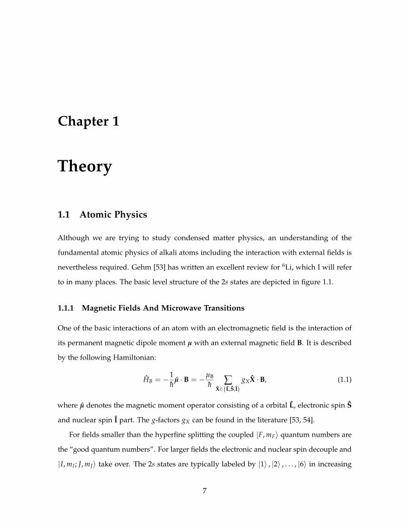
1.1 Atomic Physics
Although we are trying to study condensed matter physics, an understanding of the
fundamental atomic physics of alkali atoms including the interaction with external fields is
nevertheless required. Gehm [53] has written an excellent review for 6Li, which I will refer
to in many places. The basic level structure of the 2s states are depicted in figure 1.1.
1.1.1 Magnetic Fields And Microwave Transitions
One of the basic interactions of an atom with an electromagnetic field is the interaction of
its permanent magnetic dipole moment µ with an external magnetic field B. It is described
by the following Hamiltonian:
HB = −1h
µ · B = −µB
h ∑X∈L,S,I
gXX · B, (1.1)
where µ denotes the magnetic moment operator consisting of a orbital L, electronic spin S
and nuclear spin I part. The g-factors gX can be found in the literature [53, 54].
For fields smaller than the hyperfine splitting the coupled |F, mF〉 quantum numbers are
the “good quantum numbers”. For larger fields the electronic and nuclear spin decouple and
|I, mI ; J, mJ〉 take over. The 2s states are typically labeled by |1〉 , |2〉 , . . . , |6〉 in increasing
7

F=3/2
F=1/2
F=3/2
F=1/2
F=3/2
F=1/2
F=5/2
22S1/2
22P1/2
22P3/2
67
0.9
77
rnm
67
0.9
92
rnm
228.20526rMHz
26.1rMHz
4.4rMHz
Ram
an
(-7
rGH
z)
Slo
werr
(-8
00
rMH
z)
MO
Tr(
-33
rMH
z)
Pum
pr(
0rM
Hz)
r
Repum
pr(
-33
rMH
z)
10
.05
6rG
Hz
Figure 1.1: Level structure of the n = 2 states of 63Li and some of the laser detunings used in the
experiment
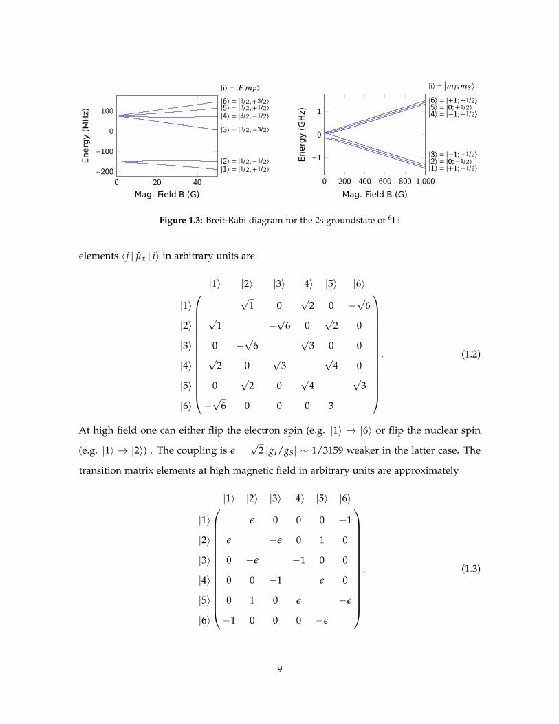
energy (see figure 1.2). The Breit-Rabi diagram for the groundstate of 6Li is shown in figure
1.3.
Transitions between the hyperfine states can be driven by applying an oscillation mag-
netic field perpendicular to the quantization axis. In our experiment this field is generated
by a single loop microwave antenna. Since the wavelength at 228 MHz is 1.3 m and therefore
a lot larger than the distance of the antenna to the atoms, the magnetic field profile is
identical to that of a loop driven with constant current. A microwave field in this orientation
can change the magnetic quantum number by ±1. At low field the relative transitions matrix
Figure 1.2: Quantum numbers of the 2s groundstate of 63Li in low and high magnetic field
8
0 20 40
−200
−100
0
100
|1⟩ = |1/2,+1/2⟩|2⟩ = |1/2,−1/2⟩
|3⟩ = |3/2,−3/2⟩|4⟩ = |3/2,−1/2⟩|5⟩ = |3/2,+1/2⟩|6⟩ = |3/2,+3/2⟩|i⟩ = |F,mF ⟩
Mag. Field B (G)
Energy(M
Hz)
0 200 400 600 800 1,000
−1
0
1
|1⟩ = |+1;−1/2⟩|2⟩ = |0;−1/2⟩|3⟩ = |−1;−1/2⟩
|4⟩ = |−1;+1/2⟩|5⟩ = |0;+1/2⟩|6⟩ = |+1;+1/2⟩|i⟩ =
∣∣mI ;mS⟩
Mag. Field B (G)
Energy(GHz)
Figure 1.3: Breit-Rabi diagram for the 2s groundstate of 6Li
elements 〈j | µx | i〉 in arbitrary units are
|1〉 |2〉 |3〉 |4〉 |5〉 |6〉
|1〉√
1 0√
2 0 −√
6
|2〉√
1 −√
6 0√
2 0
|3〉 0 −√
6√
3 0 0
|4〉√
2 0√
3√
4 0
|5〉 0√
2 0√
4√
3
|6〉 −√
6 0 0 0 3
. (1.2)
At high field one can either flip the electron spin (e.g. |1〉 → |6〉 or flip the nuclear spin
(e.g. |1〉 → |2〉) . The coupling is ε =√
2 |gI/gS| ∼ 1/3159 weaker in the latter case. The
transition matrix elements at high magnetic field in arbitrary units are approximately
|1〉 |2〉 |3〉 |4〉 |5〉 |6〉
|1〉 ε 0 0 0 −1
|2〉 ε −ε 0 1 0
|3〉 0 −ε −1 0 0
|4〉 0 0 −1 ε 0
|5〉 0 1 0 ε −ε
|6〉 −1 0 0 0 −ε
. (1.3)
9

1.1.2 Light-Matter Interaction
An atom can also be coupled to an oscillating electric field. The Hamiltonian describing a
single atom and a time-varying driving electromagnetic field can be separated into three
terms
H = HA + HL + VAL, (1.4)
where HA is the atomic Hamiltonian, HL describes the electromagnetic field (i.e. the laser),
and the interaction VAL between the two. For this work it is sufficient to consider the driving
field as a classical plane wave.
E(r, t) =12E exp (−i (ωLt− k · r)) + c.c. (1.5)
This is justified for coherent states [55]
|α〉 = exp
(−|α|
2
2
)∞
∑n=0
αn√
n!|n〉 (1.6)
with large photon numbers. Here |n〉 denotes photon number state in a single mode, also
known as Fock state. Coherent states are an excellent approximation for laser fields used in
our experiment. In addition, for large average photon numbers the term HL can be left out
of equation (1.4) since the overall photon number stays approximately constant.
Atoms couple to the electric field dominantly via an (induced) electric dipole, so that
the interaction reads [56]
VAL = −d · E(r, t) = er · E(r, t). (1.7)
Contributions from higher electric or magnetic multipoles are suppressed and only play
a role, when the direct transition is dipole forbidden, e.g. for microwave transitions or in
alkali-earth atoms.
10
1.1.2.1 Two-Level Atom
If a groundstate |1〉 only couples to one excited state |2〉, the atom can be modeled as a
two-level system. In the two-level approximation the atomic Hamiltonian reduces to
HA = hωA |2〉 〈2| , (1.8)
where the hωA is equal to the energy difference between the two states. This simplification
is valid if all other excitation and decay channels can be neglected.
For now it will be assumed that the electric field does not vary over the length scale of
an atom, so that we can approximate exp(ik · r) ≈ 1. This approximation is called the dipole
approximation.
The situation can be simplified even more if all atomic physics details of the light-matter
interaction (like the exact atomic wavefunction or polarization of the laser) are condensed
into the matrix elements of the dipole operator µi,j = 〈i| d |j〉, which can be calculated or
found in the literature [57]. The total Hamiltonian for the two-level system with the matrix
elements µ = µ1,2 = µ∗2,1 reads [58]
H = hωA |2〉 〈2| −12(µ |1〉 〈2|+ µ∗ |2〉 〈1|) (E exp (−iωLt) + E∗ exp (+iωLt)) . (1.9)
To solve the time dependent Schrödinger equation
ihddt|ψ〉 = H |ψ〉 , (1.10)
we rewrite the equations in the basis of the bare atomic states
|ψ(t)〉 = c1(t) |1〉+ c2(t) |2〉 .
Additionally, by going into the rotating frame [59] of the driving field the equations of motion
of the transformed amplitudes read
ic1(t) = − (E exp(−2iωLt) + E∗) µ
2hc2(t) (1.11)
ic2(t) = −δc2(t)− (E + E∗ exp(2iωLt))µ∗
2hc1(t).
11

In the near-resonant case we can neglect the terms oscillating at 2ωL, since the important
dynamics happen on a much slower timescale. This approximation is called the rotating
wave approximation, which is valid as long as δ ωL, ωA. Equations (1.11) can be rewritten
as an effective Hamiltonian
Heff = −hδ |2〉 〈2| − h2(Ω |1〉 〈2|+ Ω∗ |2〉 〈1|) (1.12)
with the Rabi frequency
Ω =µEh
. (1.13)
In this form the dynamics do not depend on the microscopic details of the interaction, only
on the Rabi frequency.
The general solutions in the rotating frame for the initial conditions c1(0) = 1, c2(0) = 0
and in the rotating wave approximation are given by
c1(t) = exp(
iδ
2t)(
cos(
12
Ω′t)− i
δ
Ω′sin(
12
Ω′t))
(1.14)
c2(t) = i exp(
iδ
2t)
ΩΩ′
sin(
12
Ω′t)
,
where the generalized Rabi frequency is given by
Ω′ =√
δ2 + |Ω|2. (1.15)
Experimentally more relevant is the time-evolution of the populations in the bare states
ρjj = |〈j | j〉|2
ρ22(t) =(
ΩΩ′
)2
sin2(
12
Ω′t)
(1.16)
ρ11(t) = 1− ρ22(t).
These solutions describe oscillations is the atomic population at the generalized Rabi
frequency, the Rabi oscillations.
Instead of continuously driving the system it is also possible to introduce transitions via
a single pulse. A short on-resonant (δ = 0) pulse Ω(t) with the area∫ ∞−∞ Ω(t)dt = π (called
12

a π-pulse) exchanges the population in the two bare states. This can be used to transfer
population to an excited state. A π/2-pulse creates a coherent superposition of the two
states.
1.1.2.2 Dressed States
For numerical calculations it is often easier to write the Hamiltonian (1.12) in matrix form
in the bare basis |1〉 = (1, 0), |2〉 = (0, 1)
H = −h
δ Ω2
Ω∗2 0
. (1.17)
The eigenstates of the coupled two-level systems, the dressed states, are given by
|−〉 = N−(|1〉 − Ω∗
δ + Ω′|2〉)
(1.18)
|+〉 = N+
(δ−Ω′
Ω∗|1〉+ |2〉
)with the energies
E± = − h2(δ±Ω′
)(1.19)
and normalization constants N±. The detuning dependence of their energies is depicted in
figure 1.4.
1.1.2.3 Dipole Force
In the far-detuned limit δ Ω (while still in the regime where the rotating wave approxi-
mation is valid) the dressed states
|−〉 ≈ |1〉+ 12
Ωδ|2〉 , |+〉 ≈ −1
2Ωδ|1〉+ |2〉
and the generalized Rabi frequency
Ω′ = δ +12|Ω|2
δ2 +O( |Ω|4
δ4 )
13
−4 −3 −2 −1 0 1 2 3 4
−4−3−2−101234
|1⟩
|2⟩
Detuning δ/Ω
EnergyE
/Ω
|+⟩|−⟩
Figure 1.4: Dressed state energies for varyingdetuning
0
0.20.40.60.81
P opulation
|⟨1 |1⟩|2|⟨2 |2⟩|2
−30 −20 −10 0 10 20 30
−10−50
5
10
Time tΩ
Detuningδ
/Ω
Figure 1.5: Populations during a rapid adia-batic passage
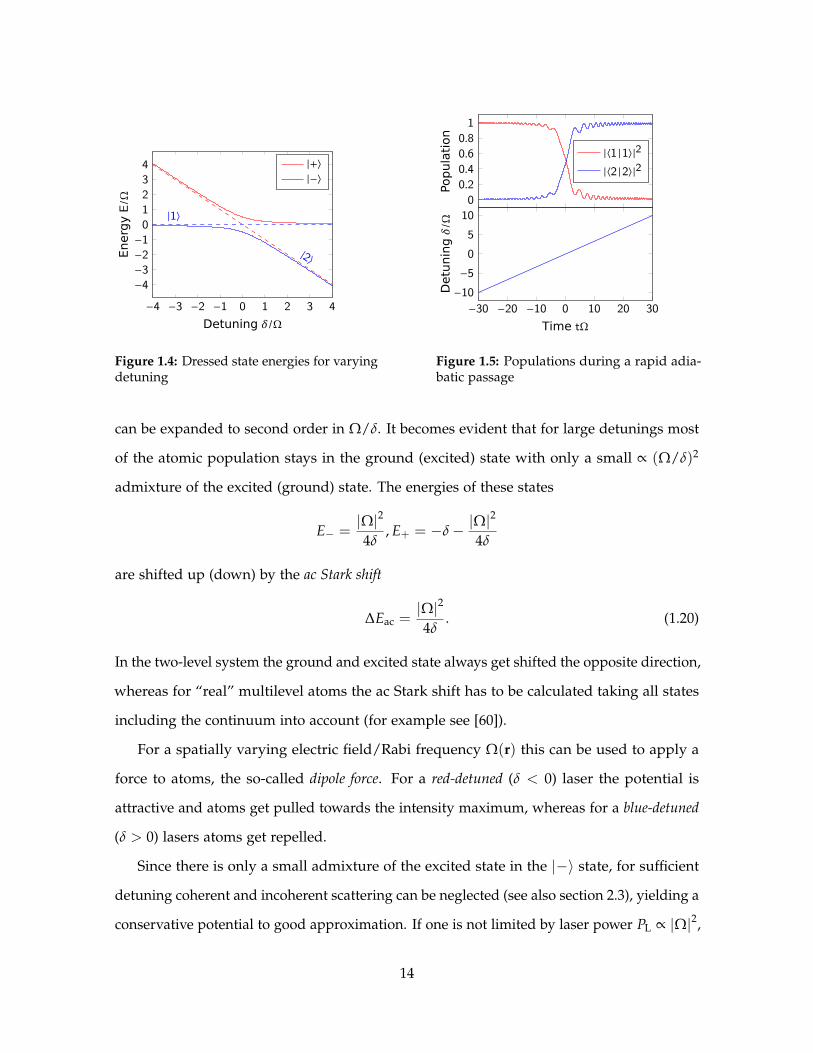
can be expanded to second order in Ω/δ. It becomes evident that for large detunings most
of the atomic population stays in the ground (excited) state with only a small ∝ (Ω/δ)2
admixture of the excited (ground) state. The energies of these states
E− =|Ω|2
4δ, E+ = −δ− |Ω|
2
4δ
are shifted up (down) by the ac Stark shift
∆Eac =|Ω|2
4δ. (1.20)
In the two-level system the ground and excited state always get shifted the opposite direction,
whereas for “real” multilevel atoms the ac Stark shift has to be calculated taking all states
including the continuum into account (for example see [60]).
For a spatially varying electric field/Rabi frequency Ω(r) this can be used to apply a
force to atoms, the so-called dipole force. For a red-detuned (δ < 0) laser the potential is
attractive and atoms get pulled towards the intensity maximum, whereas for a blue-detuned
(δ > 0) lasers atoms get repelled.
Since there is only a small admixture of the excited state in the |−〉 state, for sufficient
detuning coherent and incoherent scattering can be neglected (see also section 2.3), yielding a
conservative potential to good approximation. If one is not limited by laser power PL ∝ |Ω|2,
14

the excited state population can be reduced by detuning further, because ∆Eac ∝ δ−1 decays
more slowly than the ∝ δ−2 dependence of the population admixture. The full expression
for the dipole force without the rotating wave approximation is given in 1.79.
1.1.2.4 Rapid Adiabatic Passage
The coupling |1〉 and |2〉 via the dressed states (1.18) can be used to move population from
on state into another. This technique is more robust against uncertainties in detuning,
Rabi frequency, and timing than a π-pulse (see 1.1.2.1). If the detuning is ramped slowly
compared to the splitting Ω of the avoided crossing, the atom adiabtically follows the |−〉
state from |−(δ = −∞)〉 = |1〉 to |−(δ = +∞)〉 = |2〉 (see figure 1.5). This procedure is
called a rapid adiabatic passage and is used in several places in our experiment, for example
to reliably transfer population into excited hyperfine states of the groundstate manifold.
The condition for a linear sweep δ(t) = αt to be adiabatic is given by the Landau-Zener
criterion [61, 62]|Ω|2ddt δ(t)
1. (1.21)
This also gives this technique its alternative name, a Landau-Zener sweep.
1.1.2.5 Spontaneous Emission
The formalism described in 1.1.2.1 is sufficient to describe coherent dynamics, but is
inconvenient for including spontaneous emission. Better suited are density matrices [63], a
concept from quantum statistical mechanics, that allows to “trace out” unwanted states of
the system, for example the modes into which a photon is spontaneously emitted. Formally
density matrices are defined as
ρ = ∑i
pi |ψi〉 〈ψi| , (1.22)
where |ψi〉 is a “pure” state and pi the probability to find the system in this state.
15

The density matrix of a two-level atom is given by
ρ =
|c1|2 c1c∗2
c∗1c2 |c2|2
(1.23)
and its equation of motion by [59]
ρ11 = γρ11 −i2(Ωρ12 −Ω∗ρ21) (1.24)
ρ22 = −γρ22 +i2(Ωρ12 −Ω∗ρ21)
ρ12 = −(γ
2+ iδ
)ρ12 + i
Ω∗
2(ρ22 − ρ11)
ρ21 = −(γ
2− iδ
)ρ21 + i
Ω∗
2(ρ22 − ρ11) .
These equations are also known as the optical Bloch equations and include decay and dephas-
ing caused by finite excited state lifetime giving rise to the natural linewidth γ.
In steady state (ρ→ 0) the excited state population is given by
ρ22 =s0/2
1 + s0 + (2δ/γ)2 , (1.25)
with the on-resonant saturation parameter
s0 = 2|Ω|2
γ2 . (1.26)
For the every day lab use it is often more convenient to write the on-resonant saturation
parameter [57]
s0 ≡I
Isat
as the ratio of the light intensity I to the saturation intensity given by
Isat =2π2
3hcγ
λ3 . (1.27)
The excited state population (1.25) can also be written in a dimensionless form
ρ22 =12
s1 + s
, (1.28)
16

with the generalized saturation parameter
s ≡ s0
1 + (2δ/γ)2 (1.29)
As a function of the detuning δ equation (1.25) follows a Lorentzian profile with a
FWHM of γ′ = γ√
1 + s0. When driven with a large Rabi frequency Ω the width increases
from the natural linewidth γ. This effect is known as power broadening. Another important
feature of equation (1.25) is that the excited state population saturates at ρ22 → 12 for δ = 0
and Ω→ ∞. In other words it is not possible to create a steady state population inversion
in a two level system.
In the weak driving limit the amount of population is the excited state is proportional to
the saturation parameter s
ρ22 =12
s +O(s2) =Ω2
γ2 + (2δ)2 +O(Ω4). (1.30)
Hence, the exited state population can be kept small by either detuning or by reducing
the incident laser power. In both cases the total rate at which a driven atom is scattering
photons (coherently and incoherently) is given by
γS = γρ22. (1.31)
Each time an atom absorbs a photon it gets a directed momentum kick hkL, the sponta-
neous emission on the other hand is uniform over the whole 4π solid angle. So on average
the momentum of an atom is increasing by hkLγρ22t with gives rise to the radiation force
Frad = hkLγρ22. (1.32)
Together with the dipole force (1.20), the radiation force set the foundation for all laser
cooling and trapping experiments.
17

Relative distance
Energy
open channelclosed channel
Figure 1.6: Simplified two-channel model for a Feshbach resonance (from [1])
1.2 Feshbach Resonances
Feshbach resonances offer an unique way to tune and control the interactions between
particles. Köhler et al. [64] and Chin et al. [1] have written an excellent review paper on the
physics of Feshbach resonances.
If the energy of the two colliding atoms is near a molecular bound state (see figure 1.6),
the scattering between the two is resonantly enhanced. For atoms with non-zero nuclear
spin the magnet moment of the dimer differs from the one of a bare atom. The relative
position of the molecular bound state with respect to the atomic energies can therefore be
tuned with an external static magnetic field.
Near the s-wave scattering resonance (ignoring inelastic decay channels) the scattering
length can be parametrized by [65]
a(B) = abg
(1− ∆
B− B0
), (1.33)
with the background scattering length abg, the magnetic field where the resonance appears
B0, and the width of the resonance ∆. For homo-nuclear Feshbach molecules the binding
energy of the dimers near the resonance (a > 0) can be approximated by
Eb =h2
2ma2. (1.34)
The molecules are typically in their highest rovibrational state, which has an extent of ∼a
and a dimer-dimer scattering length of add = 0.6a [66].
18

−4,000
−2,000
0
2,000
4,000
543
.3
689
.7
809
.8
832
.2
Scatteringlength
a/a
0
|1⟩+ |2⟩|2⟩+ |3⟩|1⟩+ |3⟩
0 100 200 300 400 500 600 700 800 900 1,000 1,100 1,200−100
−50
0
Magnetic Field (G)
Boundstate
energy
EB(M
Hz)
Figure 1.7: Scattering length and molecular binding energy for 63Li
In fermionic 63Li several resonances between different hyperfine states have been observed
(see figure 1.7, data from [67]). The broad resonance between the |1〉 and |2〉 states at
B0 = 832.18(8)G with a width of ∆ = 262.3(3)G [67] (see 1.1.1 for labeling of the states) is
most commonly used. Near this resonance there are further resonances between the |2〉 and
|3〉 (B0 = 809.76(5)G [67]) states and |1〉 and |3〉 states (B0 = 689.68(8)G [67]). This makes
63Li a perfect candidate to study three-state systems with tunable interactions [68].
A narrow (∆ = 0.1 G [1]) resonance at B0 = 543.26(10)G [69] between |1〉 and |2〉 is
less frequently used directly, but it provides a zero-crossing of the scattering length at
Ba=0 = 527.5(2)G [70, 71]. This zero-crossing allows us to turn off interactions between the
|1〉 and |2〉 states to study non-interacting Fermi gases.
On the repulsive side (a > 0) of the 830 G resonance molecule formation can occur via
inelastic three-body collisions. For bosonic atoms this causes large losses which limit the
usefulness of the Feshbach resonance [72], but for fermions the relaxation to more deeply
bound molecules is suppressed by the Pauli exclusion principle [66]. We have used this fact
to create a molecular condensate of Li2 dimers (see 3.36).
19

1.2.1 Feshbach Resonances In Reduced Dimensions
With ultracold atoms in optical traps it is possible to study lower dimensional physics. For
example, in an ellipsoidal optical dipole trap or in “tubes” created by a two-dimensional
optical lattice created by two orthogonal lattices the system behaves effectively as a one-
dimensional system. Because the trap frequencies in the transverse/radial directions are
significantly higher than in the longitudinal/axial direction, the scattering into final states
with excitations along the radial are suppressed.
The coupling constant g1d replaces the three-dimensional scattering length in an effective
Hamiltonian in one-dimension. It exhibits a singularity similar to the conventional Feshbach
resonance. This confinement induced resonance [73] appears at a slightly shifted magnetic
field [74, 75].
Two dimensional systems exhibit a similar behavior [76].
In three dimensional optical lattices, strong interactions between two atoms on a single
lattice site alter the energy levels. If the scattering length a becomes comparable to the
extent of the wavefunction (i.e. the harmonic oscillator length aQHO (1.36) in deep lattices)
the energy levels in the trap shift [77] due to coupling between different bands. This has
been demonstrated experimentally by Stöfele et al. [78]. Strong interactions need be taken
into account, when the system should be approximated by a Hubbard model (see 1.5.4).
These effects can be incorporated into a generalized Hubbard model for both atoms and
molecules [79, 80].
1.3 Quantum Harmonic Oscillator
The basic problem of a quantum harmonic oscillator is omni-present in physics (e.g. [81]).
Since most optical traps can be approximated as a harmonic trap near their minimum,
harmonic oscillators are of great importance for the understanding the physics of trapped
ultracold atoms. Especially for the Raman cooling technique (see 2) the quantized motional
states of trapped atoms are an essential ingredient.
20

1.3.1 One-Dimensional Harmonic Oscillator
The Hamiltonian for a single particle of mass m in a harmonic oscillator potential with a
trap frequency ω is given by
H =p2
2m+
12
mω2 x2. (1.35)
It is possible to make it dimensionless by rewriting the position in multiples of the harmonic
oscillator length
aQHO =
√h
mω(1.36)
and rescaling the energy by hω. The eigenfunction of the quantum harmonic oscillator in
position space are
ψν(x) =
√1
2nν!
(mω
hπ
)1/4exp
(− 1
2hmωx2
)Hν
(√mω
hx)
, (1.37)
where ν = 0, 1, . . . , ∞ labels the vibrational levels and Hν(x) are Hermite polynomials [82].
The energy levels in a harmonic oscillator
En = hω
(ν +
12
)(1.38)
are equally spaced by hω.
Alternatively (1.35) can be solved by introducing the latter operators a and a†, so that
x =aQHO√
2
(a† + a
)p =
ih√2aQHO
(a† − a
). (1.39)
With those operators the Hamiltonian reads
H = hω
(n +
12
), (1.40)
where the number operator is given by n = a† a. It counts the number of excitations in the
oscillator, whereas a† (a) creates (annihilates) an excitation. The normalized eigenstates (also
known as Fock states) are given by
|ν〉 =(a†)n
√n!|0〉 , (1.41)
21

with the vacuum state |0〉.
1.3.2 Ensembles In A Harmonic Oscillator
If we add multiple indistinguishable particles, the physics depends on the quantum statistics
of the particles. Ensembles of non-interaction bosons (integer total spin) or fermions (half-
integer total spin) are described by the Bose distribution and the Fermi-Dirac distribution
respectively. The fraction of the population found occupying an energy level Ei is given
by [63]
nBF(Ei) =
1exp ((Ei − µ) / (kBT))∓ 1
. (1.42)
The chemical potential µ is implicitly given by the normalization condition ∑i n(Ei) = N
with the total atom number N.
In the limit of large numbers and when the “discrete-ness” of the trap levels does not
play a role kBT hωi, one can apply the Thomas-Fermi approximation and introduce the
number density in phase-space [83]
fBF(r, p) =
1
exp((
p2
2m + V(r)− µ)
/ (kBT))∓ 1
. (1.43)
Again, the chemical potential is given by the normalization condition
NBF=
1(2πh)3
∫d3r d3p fB
F(r, p). (1.44)
The real (or momentum) space density distribution follows by integrating over the unwanted
phase-space dimension [84]
nBF(r) =
1(2πh)3
∫d3p fB
F(r, p) = ± 1
λ3 Li3/2
(± exp
(µ−V(r)
kBT
)), (1.45)
with the thermal wavelength given by λ =√
2πh2/(mkBT).
For a three-dimensional anisotropic harmonic oscillator V(r) = ∑3i=1
12 mω2
i r2i (with the
geometric mean ω3 = ∏3i=1 ωi) the integral in (1.44) can be evaluated as well, yielding
N(QHO)BF
= ±(
kBThω
)3
Li3
(± exp
(µ
kBT
)), (1.46)
22

where Liν(z) denotes the polylogarithm [82].
1.3.2.1 Thermal Cloud
In the high-T limit we reproduce the classical result (i.e. ignoring ∓1 in (1.43) or assuming
the Maxwell-Boltzmann distribution). In this case (1.46) simplifies to
Nth =
(kBThω
)3
exp(
µ
kBT
), (1.47)
giving rise to
µth = kBT log
(1N
(hω
kBT
)3)
(1.48)
and
nth(r) =N
π3/2σ3 exp
(−
3
∑i=1
(ri
σi
)2)
, (1.49)
where σ3 = ∏3i=1 σi denotes the geometric mean of the rms cloud sizes
σi =√
2kBT/(mω2i ). (1.50)
Therefore the FWHM cloud size is
d(i)th = 2σi√
log 2 ≈ 2.35
√kBTmω2
i. (1.51)
At first it seems surprising that the cloud size does not depend on the atom number, but an
ensemble off non-interacting particles without spin statistics behaves identically to a single
particle.
In a harmonic trap the phase space density for a thermal gas, an important quantity for
optimizing evaporative cooling, is given by
ρ = N(
hω
kBT
)3
. (1.52)
23

1.3.2.2 Degenerate Fermi Gas
For a fully degenerate gas at T = 0 the normalization defines the Fermi energy
EF = µ(T = 0) = hω3√
6N, (1.53)
the highest occupied energy in the system. The in-trap real-space density near the trap
center (ri Ri) is then given by
n(T=0)F (r) ≈ 8N
π2R3
(1−
3
∑i=1
r2i
R2i
)3/2
, (1.54)
with the Fermi radii Ri =√
2EF/(mωi)2 and their geometric mean R. This can also be derived
using the local density approximation with a spatially dependent chemical potential/Fermi
energy E(free)F (r) = EF − V(r) with the Fermi energy for a untrapped Fermi gas E(free)
F =
h2
2m
(3π2n
)3/2 [63], where the density is assumed to be locally constant n ≈ n(r).
The FWHM of the exact solution of (1.45) is given by
d(i)F (T = 0) = 1.22Ri ≈ 1.72
√EF
mω2i
. (1.55)
Using definition (1.53) and the Fermi temperature TF = EF/kB equation (1.46) can be
rewritten in a universal form to simplify numerical calculations(TTF
)3
Li3
(− exp
(µ
EF
TF
T
))= −1
6. (1.56)
The atom number dependency now is absorbed into the Fermi energy.
Equation (1.48), which is a good approximation in the high temperature limit (T & 0.5TF),
can be rewritten in a similar fashion
µ(T & 0.5TF)
EF≈ T
TFlog
(16
(TF
T
)3)
. (1.57)
The low (but finite) temperature expansion this gives a Sommerfeld-like expression [83] for
the chemical potential inside a harmonic trap
µF(T TF)
EF≈(
1− π2
3
(TTF
)2)
. (1.58)
24

0 0.5 1
−2
−1
0
1
Temperature T/TF
Chemical p
otentialµ
/EF
ExactLow-THigh-T
Figure 1.8: Chemical potential for a Fermigas in a harmonic trap
−2 0 2
0
0.5
1
Position r/R
Density
n(r)(a.u.)
0.00.51.0
Figure 1.9: Density profiles for different T/TF
The exact solution and the approximations are all plotted in figure 1.8 in agreement with
Butts et al. [83].
1.3.2.3 Bose-Einstein Condensate
While fermions all occupy different states, at T = 0 all atoms in a non-interacting Bose-
Einstein condensate occupy the ground of the trap. For a harmonic trap the wavefunctions
are given by equation (1.37). Therefore the density distribution in the ground state ν = 0 is
n(T=0)B (r) = N
(mω
hπ
)3/2
exp
−∑(
ri
σ(i)B
)2 (1.59)
with an rms cloud size equal to the harmonic oscillator length
σ(i)B =
√h
mωi(1.60)
and FWHM of
d(i)B (T = 0) = 2σ(i)B
√log 2 ≈ 1.67
√h
mωi. (1.61)
The cloud size of a Bose-Einstein condensate has a weaker dependence on the trap
frequency (∝ ω−1/2i ) than for the degenerate Fermi gas or a thermal cloud (∝ ω−1
i ) . A
more detailed description of trapped (and also interacting) Bose-Einstein condensates can
25

−2 −1 0 1 2
0
0.5
1
1/e2
1/pe
Radius r/w0
Intensit y
I/I 0
Figure 1.10: Radial intensity profile of a Gaus-sian beam at the focus
−3 −2 −1 0 1 2 3
0
1
2
3
p2
Position z/zR
Waistw
/w0
Figure 1.11: Gaussian beam waist along theoptical axis
be found in Ketterle et al. [85].
1.4 Optical Potentials
1.4.1 Gaussian Beams
Laser beams can be well described as Gaussian beams. Gaussian beams are the solutions to
the paraxial scalar Helmholtz equation and their electric field for a beam propagation along
the z-axis and focused at is given by [86]
E(ρ, z) = E0w0
w(z)exp
(−(
ρ
w(z)
)2
− ik(
z− ρ
2R(z)
)+ iζ(z)
), (1.62)
with a Gaussian beam waist
w(z) = w0
√1 +
(z
zR
)2
. (1.63)
The electric field here is written as a complex field, but the physical field is only its the real
part E(ρ, z) = Re(E(ρ, z
).
The Gaussian beam waist is the radius, where the electric field amplitude has dropped to
1/e and the intensity to 1/e2 (see figure 1.10). The distance zR where the waist has increased
26

by a factor of√
2 of its minimum w0 is called the Rayleigh length
zR =πw2
0λ
. (1.64)
The radius of curvature of the wave front is
R(z) = z(
1 +( zR
z
)2)
. (1.65)
Another related quantity is the Gouy phase
ζ(z) = arctanz
zR, (1.66)
which describes the fact that the field undergoes a π phase shift when going through a focus.
This plays a significant role in the design of resonators, but is irrelevant for the intensity
profiles of propagating Gaussian beams.
In the far field (z zR) the beam is well described by geometric optics: the beam radius
increases linearly and gives rise to a divergence angle (half-angle)
θ =w0
zR. (1.67)
The radius of curvature approaches R(z zR) = z as one would expect geometrically.
The intensity profile of a Gaussian beam is given by
I(ρ, z) = I0
(w0
w(z)
)2
exp
(−2(
ρ
w(z)
)2)
. (1.68)
For a known total power P the peak intensity can be expressed as
I0 =2P
πw20
. (1.69)
The paraxial scalar Helmholtz equation is valid as long as the numerical aperture of
the angle is small and as long as polarization effects do not play a role. For example when
projecting a pattern through a high numerical aperture objective lens this assumption can be
violated and the contrast of the pattern reduced. The numerical aperture (NA) is defined as
NA = n sin θ, (1.70)
27

0 0.5 1 1.5 2
0
0.25
0.5
0.75
1
Annular clip radius rclip/w0
PowerP
/P0
−2 −1 0 1 2
Linear clip xclip/w0
Figure 1.12: Transmitted power of a clipped Gaussian beam
where n is the index of refraction of the medium (typically n ∼ 1.0 for air/vacuum) and θ is
the largest angle ray that can be collected by the imaging system. In the paraxial limit the
NA can also be written as the ratio of focal length f and the diameter D of entrance pupil:
NA = n f2D .
1.4.1.1 Beam Collimation
A Gaussian beam is said to be collimated, when the wavefront is flat, which is the case at
the focus of the beam (limz→0 R(z) = ∞). It is a common misconception that a beam can be
collimated by focusing at “infinity”. In fact with a lens of focal length f a Gaussian beam
of given waist w0 and Rayleigh length zR can only be focused/collimated at a maximum
distance of
dmax = f(
fzR
+ 1)
fzR≈ f 2
zR, (1.71)
which for typical fiber collimation parameters is roughly equivalent to one meter. Doing so
will result in a more tightly focused waist that is 1/√
2 smaller as the naively expected waist
of w′0 = λ fπw0
. A consistent way is to collimate the beam interferometrically, for example
using a shearing interferometer. A more detailed discussion based on the transfer matrix
method can be found in A.2.1.
28

1.4.1.2 Clipped Beams
The aperture of optical components in the experiment is always limited. This aperture could,
for example, be the active area of an acousto-optical modulator, an iris, a vacuum window
or even just the clear aperture of a lens. In case of a Gaussian beam with a waist of w0 and
a circular aperture with radius rclip that is centered on the optical axis and only transmits
the part of the beam where ρ < rclip, the fraction of the transmitted power is given by
PP0
= exp
(−2(
rclip
w0
)2)
. (1.72)
If, on the other hand, the beam is clipping on a linear edge, so that only light in the
region x > xclip and y ∈ R is transmitted, the fraction is given by
PP0
=12
(1 + erf
(√2xclip
w0
)), (1.73)
with the error function erf(x) [82]. This can be useful to measure the waist of a laser beam
by moving a razor blade into the beam and measuring the transmission as a function of the
razor blade position. This method is particularly useful for beams larger than the typical
size of a CCD/CMOS based laser beam profiler. The fractional transmitted power for the
two cases of clipping is depicted in figure 1.12.
1.4.1.3 Measuring Beam Parameters
The quality of a laser beam is often quantified by the M2 parameter [87], which is defined as
M2i =
π
λd(ISO)
i Θ, (1.74)
where λ denotes the wavelength, d(ISO) the beam diameter at the focus, and Θ the full
far-field divergence angle. The International Organization of Standardization defines the
beam diameter along the i ∈ x, y axis (which are assumed to be the principal axes) as
d(ISO)i = 4σi, (1.75)
29

−20 0 20 40
300
400
500
Position (cm)Waist(µm)
Figure 1.13: Example of measured beam waists at different positions and fitted data with w0 =274(1) ¯m and M2 = 0.98(1).
with the square of the standard deviation of the power/intensity distribution
σ2x =
⟨x2 − 〈x〉2
⟩=
x (x2 − 〈x〉2
)I(x, y)dx dy/
xI(x, y)dx dy (1.76)
and σ2y at the focus of each direction. This definition of the beam diameter is sometimes
also called D4σ.
For a Gaussian beam described by (1.68) the beam diameter is
d(ISO) = 2w0 (1.77)
and together with the far-field divergence Θ = 2θ of (1.67) this yields an
M2 = 1.
This is the lowest physically possible value. For a non-diffraction limited Gaussian spot
with spot size w′ in the focus
M′2 =w′2
w20≥ 1.
Determining the beam parameters the ISO norm 11146-1 [87] requires the beam profile
to be measured five times near the focus (|z| < zR) and five times in the far-field (|z| > zR).
The beam parameters can then be extracted using a non-linear fit of the data points (see
figure 1.13). We found that using the second moment to obtain a beam diameter gave more
reliable results than trying to fit a Gaussian distribution to the profiles acquired with a
30

−4 −2 0 2 4
−2
−1
0
1
2
z/zRx/w0
Figure 1.14: Intensity distribution of a Gaussian beam propagating along the z axis
CMOS beam profiler.
1.4.2 Travelling Wave Potentials
As seen in section 1.1.2.3 a laser beam far detuned from the atomic resonance(s) can provide
a conservative potential. The strength of the potential is proportional to the intensity of
the laser beam (1.68). A single red-detuned Gaussian beam alone can already confine
sufficiently cold atoms in all three spatial dimensions [88], since they get attracted to the
intensity maximum (see figure 1.14). The potential then has the following form
Vodt(r) = −V0
(w0
w(z)
)2
exp(−2
x2 + y2
w(z)2
). (1.78)
The rotating wave approximation used in 1.1.2.1 might not be justified for very large
detunings when ω0 + ωL ∼ ω0 −ωL. In general the trap depth taking only a single excited
state into account can be obtained with the following formula [89]:
V0 =3Pc2
w20ω3
0
(γ
ω0 −ωL+
γ
ω0 + ωL
). (1.79)
Here the counter-rotating terms are included as well and the transition matrix element is
expressed as a function of the natural linewidth γ and the transition frequency ω0. The
laser frequency is denoted by ωL. For lithium in a far off-resonant dipole potential created
by 1064 nm light the correction due to the counter-rotating term is 23%.
31

As stated above for a red-detuned laser (ωL < ω0) the potential is attractive. Repulsive
blue-detuned lasers can used for trapping as well, although this requires more complicated
setups to, for example, create light sheets [90], a doughnut beam [91], or holographically
generated traps [92].
Expanding the potential (1.78) around the minimum to second order and comparing it
to harmonic oscillator potentials VQHO(x) = 12 mω2
xx2, one can read off the trap frequencies
in the longitudinal (z) and transverse (x, y) directions:
ωodt,long,x = 2π
√1
2mV0
π2z2R= 2π
√1
2mV0λ2
π4w40
, (1.80)
ωodt,trans,y = 2π
√1m
V0
π2w20
. (1.81)
The ratio of the transverse to longitudinal trap frequency is given by
ωodt,trans,y
ωodt,long,x=√
2πw0
λ.
For typical low numerical aperture geometries w0 λ and thus the trap is very elongated.
One way around this limitation is to combine two perpendicular laser beams focused
onto the same position to form a crossed optical dipole trap [93]. This way it is possible to
achieve a nearly spherical trap. Care must be taken to avoid interference between the two
distinct beams by choosing orthogonal polarizations or better by detuning the two beams
from each other. The interference pattern is then modulated with the relative detuning (see
(1.86)) and averages out when this modulation is a lot faster than all trap frequencies.
Another possibility to avoid interference is to use a light source with a short coherence
length such as a superluminescent diode (see 3.2.4). Superluminescent diodes are best choice
of incoherent lightsources. Some other broadband lasers (e.g. pulsed lasers) might have
coherence revivals or just slowly jump between discrete modes, which could heat atoms in
the trap.
It is important to note that most of those lasers are temporarily incoherent, but spatially
single mode. Therefore different parts of the wavefront at a given z can still perfectly
32

x
y
z
dlat,1d,yθ
(a) Two interfering laser beams
x
y
z
dlat,1d,y
dlat,2d,x
λ
θ
(b) Four interfering laser beams
Figure 1.15: Geometries for standing wave potentials
interfere. This can pose a problem when an incoherent laser beam, although having short
longitudinal coherence length, reflects of a surface under a shallow angle, for example
the optical dipole trap used to transport atoms near the superpolished substrate in our
experiment (see 3.4.5 and 3.4.7).
Another concern when designing optical traps is heating caused by scattering of the
trapping laser. Although the trapping laser is usually far detuned from any atomic resonance,
the atoms can still scatter that light at a rate of [89]
γsc(r) = −Vdip(r)
h
(ωL
ω0
)3 ( γ
ω0 −ωL+
γ
ω0 + ωL
). (1.82)
This is the more general form of equation (1.31). The ratio of trap depth to scattering rate
Vdip/(hγsc) can be increased by going to longer wavelengths, although the laser power
required to achieve a given trap depth increases as well.
1.4.3 Standing Wave Potentials
The possible feature size of traps created with a single beam is limited by the numerical
aperture. To produce smaller patterns one can use two beams with a constant phase relation
and let them interfere. Rather than just adding up the intensities incoherently, the electric
fields add up coherently and form a standing wave. Its periodicity is on the order of the
wavelength with a minimum value of λ/2.
33

1.4.3.1 Two Interfering Beams
In the simplest case we have two beams with a constant phase relation. This, for example, can
be achieved by retro-reflecting a single beam back into itself. For two counter propagating
plane waves with amplitudes and polarizations Ei = εiEi, angular frequency ωi, and
wavevector ki = 2π/λi = ω/c, the complex field is given by
E(x, t) = E1 exp (ik1x− iω1t− iφ1) + E2 exp (−ik2x− iω2t− iφ2) (1.83)
or the real electric field by
E(x, t) = E1 cos (k1x−ω1t− φ1) + E2 cos (−k2x−ω2t− φ2) . (1.84)
The resulting intensity as defined via the Poynting vector [94] is
µ0cI(x, y, t) = E21 cos2 (k1x−ω1t− φ1) + E2
2 cos2 (−k2x−ω2t− φ2) +
E1 · E2 (cos ((k1 − k2) x− (ω1 + ω2) t− (φ1 + φ2)) +
cos ((k1 + k2) x− (ω1 −ω2) t− (φ1 − φ2))) . (1.85)
Let us assume that the two frequencies are almost equal ωL ≡ ω1, ω2 = ω1 + ∆ω, kL =
k1, k2 = k1 + ∆k and φ1 = 0, φ2 ≡ φ. Then the interference term can be written as
E1 · E2 (cos (2ωLt + φ + ∆kx + ∆ωt) + cos (2kLx + φ + ∆kx + ∆ωt)) .
In the short-time (∆ω−1 t ω−1L ) average the time dependencies in the incoherently
added fields drop out⟨cos2(ωit)
⟩t =
12 . The fast-oscillating term of the interference term
〈cos(2ωLt)〉t = 0 (see figure 1.16) vanishes as well, so that the intensity averaged over short
times is given by
2µ0c 〈I(x, y, t)〉t = E21 + E2
2 + 2E1 · E2 cos ((2kL + ∆k)x− ∆ωt + φ) . (1.86)
To get a stationary interference pattern, a standing wave, it is required that the fre-
quencies are equal (∆ω = 0) and that the two polarizations have a parallel component
34

0 50 100
0
2
4
Time tω1Intensity
µ0cI
/E2
I(t)⟨I (t )⟩
Figure 1.16: Time dependent intensity of two counterpropagating beams with ω2 = 1.1ω1.
(E1 · E2 6= 0). The interference contrast is simply given by the peak-to-peak modulation
h ≡ 2E1 · E2
E21 + E2
2. (1.87)
In general one does not need a retro-reflector, but can use two separate actively or
passively phase stabilized beams that intersect under an arbitrary angle θ (see figure 1.15a).
In the following sections the symmetry axis of the two beams defines the x axis and the
beams span the x− y plane with the z direction perpendicular to this plane. The standing
wave is modulated along the y direction, which will also be called the longitudinal or axial
direction. The x− z plane defines the transverse or radial directions.
In the following we will drop the assumption of infinitely large plane waves and assume
Gaussian beams with linear polarization along the z axis, but still require that w0 dlat,1d
(which could easily be violated for θ → 0, see (3.17)).
Most commonly two counterpropagating beams (θ = π/2) are used, giving rise to the
potential
V(y, ρ) = V(y, ρ) cos2(ky), (1.88)
with a slowly varying envelope
V(y, ρ) = Vlat,1d exp(−2
ρ2
w(y)2
)(1.89)
and ρ2 = x2 + z2. The second order expansion of this envelope is often called the harmonic
35

confinement.
For two coherent beams with identical wavelength λ, the intensity at the maximum is
enhanced by a factor of four over a single beam trap (independent of the angle, provided
that w0 dlat,1d)
Vlat,1d = 4V0. (1.90)
This factor originates from coherent addition of the electric fields instead of intensities as
shown explicitly for the counterpropagating case (1.86).
Only the parallel components of the wave vectors will interfere, leading to a lattice
spacing of
dlat,1d,y =12
λ
|sin θ| . (1.91)
In the limit of two counterpropagating beams (θ = π/2) the lattice spacing is λ/2, typical
for most optical lattice experiments.
An important derived quantity is the so called recoil energy
Er =h2k2‖
2m, (1.92)
where k‖ = kλ sin θ and kλ = 2π/λ. The recoil energy is the gain in kinetic energy an atom
at rest of mass m would experience, if it absorbed a photon with the momentum hk‖. For
counterpropagating beams (θ = π/2), k‖ turns into kλ.
As in section 1.4.2 the trap frequency can be read off from the quadratic term of the
expansion around the potential minimum (see also section 1.5.1.4):
ω1d,long,x = 2π
√Vlat,1d
2md2lat,1d
= 2π
√2V0
m|sin θ|
λ. (1.93)
Using the lattice recoil energy the trap frequency can also be written in a dimensionless
form ashω1d,long,x
Er= 2
√Vlat,1d
Er. (1.94)
In the direction of the strong transverse confinement (along the y axis) the geometrical
waist is still given by the beam waist w0. Thus the trap frequency in that direction just
36

0 0.25 0.5 0.75 1
0
0.5
1
Phase φ/(π/2)Relativeintensity
1−
√V1V2
/(V1+V2
)
Figure 1.17: Optical potentials for different interference contrast and relative depth
corresponds to a single beam trap with a fourfold deeper trap:
ω1d,trans,strong,y =√
4ωodt,trans = 2π
√1m
Vlat,1d
π2w20
. (1.95)
The confinement in the other transverse direction is weaker:
ω1d,trans,weak,x = 2π
√√√√ 1m
Vlat,1d
π2z2R
(12
cos2 θ +
(zR
w0
)2
sin2 θ
). (1.96)
This trap frequency approaches ω1d,trans,strong,y in the limit of two counterpropagating beams
(θ = π/2) and 2ωodt,long,x for near copropagating beams (θ → 0).
1.4.3.2 Four Interfering Beams
The situation gets more complex, when there are four laser beams involved. In typical
optical lattice experiments with two pairs (or more) of lattice beams, interference between
different axes is avoided by choosing orthogonal polarizations and sufficiently large relative
detuning. This leads to the well-known egg-crate style lattice potential.
Allowing for interference between two axes can greatly enhance the lattice depth for
a given laser power and also generate interesting lattice structures (see figure 1.17). For
example, Uehlinger et al. [17] took advantage of the mutual interference to adiabatically
double the number of lattice sites. To achieve a stationary lattice pattern, the phase between
the interfering axes needs to be actively or passively stabilized.
In general the optical potential created by two pairs of interfering plane waves of equal
37

intensity with a relative phase φ can be described by
−V(r) = V(1)lat,1d cos2 (k1 · r)+V(2)
lat,1d cos2 (k2 · r)+ 2√
V(1)lat,1dV(2)
lat,1d sin φ cos (k1 · r) cos (k2 · r) .
(1.97)
The lattice spacing in the y direction remains unchanged from the two beam interference
and is given by equation (1.91). In the perpendicular x direction the spacing is given by
dlat,2d,x =12
λ
|cos θ| . (1.98)
Overall the lattice depth is enhanced by the interference term in equation (1.97), which in
the case of perfect interference (φ = π/2) leads to
Vlat,2d = 16V0 = 4Vlat,1d. (1.99)
This is a significant improvement of the achievable trap frequency for a given laser power
and is used in our experiment to create sufficiently deep optical lattices for fluorescence
imaging (see 2.9).
Provided that the beams can be approximated as plane waves (w0 λ), the trap
frequencies on each lattice site for perfect interference (φ = π/2) are given by
ω2d,y = 2π
√2Vlat,2d
m|cos θ|
λ(1.100)
and
ω2d,x = 2π
√2Vlat,2d
m|sin θ|
λ. (1.101)
1.4.4 Noise-Induced Heating
Needing to hold atoms in an optical trap for a long time imposes stringent requirements on
the lasers. Both frequency and amplitude fluctuations in the trapping laser can motionally
excite the trapped atoms and in the worst case heat them out of the trap. Especially for
quantum simulation of the Hubbard model (see 1.5.4) one has to ensure that the atoms stay
in the lowest band of the optical lattice for the duration of the experiment.
38

Savard et al. [95] modeled the effect of the amplitude noise by looking at the rate at
which a single atom in an harmonic trap with a fluctuating trap frequency ωtrap(1 + ε(t))
gets excited. For small fluctuations the rate at which atoms get excited from the ground
vibrational state to the second excited vibrational state is
Γ(AM)ν=0→ν=2 =
π
8ω2
trapSAM(2ωtrap). (1.102)
Here SAM(2ωtrap) is the single-sided relative power-spectral density of the laser intensity
(often also called residual intensity noise, given in units of dBc/Hz) at the twice the trap
frequency. There is no contribution to heating from noise directly at the trap frequency. In
the perturbative regime modulation of the potential with even parity cannot drive transitions
between adjacent vibrational levels. Heating caused by intensity fluctuations causes an
exponential rise of the temperature since the rate increases for higher excited states ν > 0.
Another source of noise are pointing fluctuations of the trap center V(x) = 12 mωtrap(x−
εx(t))2. Besides mechanical vibrations on optical components that alter the transverse
pointing of a laser beam, frequency fluctuations of the laser itself can cause a shift in the
longitudinal position of an optical lattice. For a counterpropagating one-dimensional optical
lattice the nth lattice site is x0 = nλ/2 = πnc/ωL away from the retro-reflector. To first
order a small fluctuation δωL shifts that position by
δx = x0δωL
ωL. (1.103)
The rate at which pointing noise drives transitions between the ground and the first excited
vibrational state is [96]
Γ(XM)ν=0→ν=1 =
π
2hmω3
trapSXM(ωtrap). (1.104)
Here SXM(ω) is the power-spectral density of the position fluctuations (in units of m2/Hz)
which is connected to the frequency power-spectral density SFM(ω) (in units of (2ßHz)2/Hz)
via equation (1.103):
SXM(ω) =
(x0
ωL
)2
SFM(ω). (1.105)
The frequency fluctuations of a laser can be modelled as white Gaussian noise εω(t)
39

(up to a certain bandwidth). This kind of frequency noise corresponds to the 1/ f 2 term in
the phase noise and gives rise to a Lorentzian frequency profile with linewidth ∆ω. The
frequency noise power spectral density is given by [97]
SFM(ω) =2π
∫ ∞
0dτ cos(ωτ) 〈εω(t)εω(t + τ)〉 = ∆ω. (1.106)
Frequency noise can get converted to amplitude noise by components that have a
frequency/wavelength dependence of their transfer function (for example cavities). Unin-
tentional reflections off optical componentents can act as resonator as well.
For 6Li atoms in an optical lattice with a 1 MHz trap frequency and a distance of
10 cm from the retro-reflector created by a laser with 1 MHz linewidth and 100 dBc/Hz
residual amplitude noise would experience heating at a rate of Γ(AM)ν=0→ν=2 = 2π · 248 Hz
and Γ(XM)ν=0→ν=1 = 2π · 117 Hz. These results emphasize the importance of having lasers with
extremely low residual amplitude noise (< −130 dBc/Hz) and small distance between the
atoms and the retro reflector, when one is working with high trap frequencies. Acoustic
noise become less of a problem.
1.5 Physics Of Optical Lattices
Optical lattices are more than just arrays of microtraps. The symmetry of the system
drastically changes: the continous translation symmetry is broken by the lattice potential.
1.5.1 Band Structure Calculation
This broken symmetry changes the dispersion (i.e. relations between momentum and
energy) of a single delocalized particle in an optical lattice.
1.5.1.1 d-Dimensional Square Lattice
For infinite systems described by the Hamiltonian
H =1
2mp2 + V(r), (1.107)
40

with a potential energy term that is periodic in space
V(r) = V(r + R), (1.108)
the wavefunctions φ(n)q (r) inherit the periodicity
φ(n)q (r) = φ
(n)q (r + R) (1.109)
and can be written in the following form (known as Bloch’s theorem [98]):
φ(n)q (r) = exp
(ih
q · r)
u(n)q (r). (1.110)
Here R denotes a Bravais lattice vector. For a three-dimensional square lattice with lattice
spacing a it is given by
R = a(iex + jey + kez
)∀i, j, k ∈ Z. (1.111)
Using Bloch’s theorem, the Schrödinger equation reads
H′u(n)q (r) = E(n)
q u(n)q (r), (1.112)
with a slightly modified Hamiltonian
H′ =1
2m(p + q)2 + V(r). (1.113)
On a square lattice the periodicity of the problem suggests to switch to a d-dimensional
discrete Fourier basis to get a general solution numerically.
u(n)q (r) =
∞
∑l1=−∞
∞
∑l2=−∞
. . .∞
∑lD=−∞
c(n)q,l exp
(i
d
∑i=1
liκiri
)
V(r) =∞
∑s1=−∞
∞
∑s2=−∞
. . .∞
∑sD=−∞
Vs exp
(i
d
∑i=1
siκiri
)It can be seen that the potential term couples different l because of the exp (isiκiri) phase
factors, (i.e. resulting in off diagonal terms in the Hamiltonian matrix in the exp (iniκiri) |
41

−20
−10
0
10
20
EnergyE
/Er
V1 = 1Er
−0.5 0 0.5
Quasimomentum q/~κ
V1 = 10Er V1 = 20Er
Figure 1.18: Bandstructure of an one-dimensional lattice for various depths
i ∈ 1, 2, . . . , d , ni ∈ Z basis), but most Vr are going to be equal to zero.
V(r)u(n)q (r) = ∑
l,sVsc(n)q,l exp
(i
d
∑i=1
(li + si)κiri
)
In this basis the kinetic term turns into
12m
(p + q)2u(n)q (r) = ∑
l
d
∑j=1
h2κ2j
2m
(lj +
qj
hκj
)2
c(n)q,l exp
(i
d
∑i=1
liκiri
).
The variable q is called the quasimomentum.
1.5.1.2 One-Dimensional Lattice
In the case of a one-dimensional optical lattice, such as the lattice described in section 1.4.3.1,
the potential along the direction of the optical lattice is typically written as
−V(x) = V1 cos2(kx) = V1
(12+
14
exp (i2kx) +14
exp (−i2kx))
, (1.114)
where k = 2π/λ for counterpropagating beams or k = 2π/(2dlat,1d) in the general case (see
equation (1.91)). By substituting κ = 2k one can calculate the elements of the Hamiltonian
matrix:
42

0 5 10 15 20 25 30
−25−20−15−10−50
5
Depth V/Er
Ener gyE
/Er
Figure 1.19: Bands for various lattice depthsin an one-dimensional lattice
0 10 20 30 40 50 60 70 80 90 100
0
1
2
3
4
5
6
7
Depth V/Er
NumberofBoundstates
q= 0
q= ~κ/2√V/Er/2
N(4)bound
Figure 1.20: Number of bound states in aone-dimensional lattice
Hl,l′ =
4Er
(lj +
qjhκ
)2− V1
2 ∀l = l′
− 14 V1 |∆l| = 1
0 else
(1.115)
with a lattice recoil energy of Er =h2k2
2m = 14
h2κ2
2m . The first Brillouin zone extends from −hκ/2
to hκ/2. To perform numeric calculations the Hamiltonian matrix needs to be truncated by
only including elements for l = −lmax . . . + lmax.
For weak lattices the bands are still very similar the parabolic free particle dispersion
Efree =p2
2m
folded into the first Brillouin zone. The lattice potential then couples the quasimomentum
parabolas differing by |∆l| = 1 and opens up gaps at the intersections. Now only certain
bands of energies levels are allowed (figure 1.19), hence the name band structure . In the
limit of very deep lattices the bands become flat and approach equally spaced quantum
harmonic oscillator levels (figure 1.18).
Number Of Bound States The fact that band become flat can be used to approximate the
number of bound states in deep lattices. For a given trap depth V1 and a harmonic oscillator
43
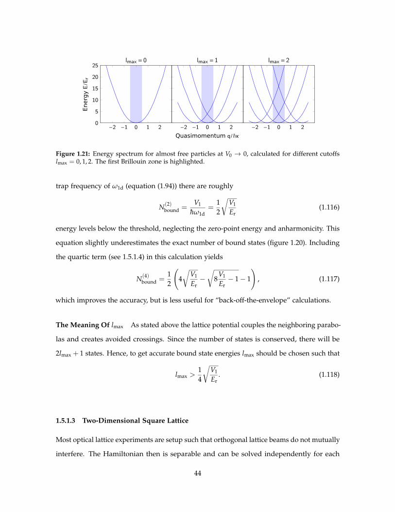
−2 −1 0 1 20
5
10
15
20
25
EnergyE
/Er
lmax = 0
−2 −1 0 1 2
Quasimomentum q/~κ
lmax = 1
−2 −1 0 1 2
lmax = 2
Figure 1.21: Energy spectrum for almost free particles at V0 → 0, calculated for different cutoffslmax = 0, 1, 2. The first Brillouin zone is highlighted.
trap frequency of ω1d (equation (1.94)) there are roughly
N(2)bound =
V1
hω1d=
12
√V1
Er(1.116)
energy levels below the threshold, neglecting the zero-point energy and anharmonicity. This
equation slightly underestimates the exact number of bound states (figure 1.20). Including
the quartic term (see 1.5.1.4) in this calculation yields
N(4)bound =
12
(4√
V1
Er−√
8V1
Er− 1− 1
), (1.117)
which improves the accuracy, but is less useful for “back-off-the-envelope” calculations.
The Meaning Of lmax As stated above the lattice potential couples the neighboring parabo-
las and creates avoided crossings. Since the number of states is conserved, there will be
2lmax + 1 states. Hence, to get accurate bound state energies lmax should be chosen such that
lmax >14
√V1
Er. (1.118)
1.5.1.3 Two-Dimensional Square Lattice
Most optical lattice experiments are setup such that orthogonal lattice beams do not mutually
interfere. The Hamiltonian then is separable and can be solved independently for each
44

lattice direction. Allowing mutual interference between two lattice axes gives rise to a
potential of the form
−V(r) = V1 cos2(k1r1) + V2 cos2(k2r2) + 2√
V1V2 sin φ cos(k1r1) cos(k2r2) =
=V1 + V2
2+
V1
4[exp (2ik1r1) + exp (−2ik1r1)] +
V2
4[exp (2ik2r2) + exp (−2ik2r2)] +
V sin φ
2[exp (ik1r1 + ik2r2) + exp (ik1r1 − ik2r2) +
exp (−ik1r1 + ik2r2) + exp (−ik1r1 − ik2r2)] , (1.119)
where V =√
V1V2 denotes the geometric mean of the two potential depths. The relative
phase between the lasers of the two axes is denoted by φ. Reading of the matrix elements,
we can write the Hamiltonian in matrix form:
Hl,l′ =
∑2j=1
(h2k2
j2m
(lj +
qjhk j
)2− Vj
2
)∀l = l′
− 12 V sin φ |∆l1| = 1∧ |∆l2| = 1
− 14 V1 |∆l1| = 2∧ ∆l2 = 0
− 14 V2 ∆l1 = 0∧ |∆l2| = 2
0 else
. (1.120)
In comparison to equation (1.120) the kinetic energy is parameterized with the laser wavevec-
tors ki. The first Brillouin zone now extends from −hki to hki.
In the special case of φ = 0 we only have terms oscillating at 2ki. Thus the primitive unit
cell is effectively halved and the Hamiltonian factorizes into two decoupled subspaces per
spatial dimension, one for even and one for odd lis. In other words, we are solving the same
problem twice, but shifted by ki/2 in quasimomentum space, and yields the same result as
the one dimensional lattice.
Similar to the one dimensional case we truncate our Hilbert space by limiting the
maximum l and numerically solve the problem by diagonalizing the truncated Hamiltonian
matrix. Figure 1.22 shows the density of states in a two dimensional lattice as a function of
the interference between the two lattice beams sin φ.
45
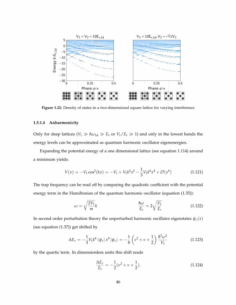
0 0.25 0.5−30−25−20−15−10−50
5
Phase φ/π
EnergyE
/Er,1d
V1 =V2 = 10Er,1d
0 0.25 0.5
Phase φ/π
V1 = 10Er,1d,V2 =p
2/2V1
Figure 1.22: Density of states in a two-dimensional square lattice for varying interference
1.5.1.4 Anharmonicity
Only for deep lattices (V1 hω1d Er or V1/Er 1) and only in the lowest bands the
energy levels can be approximated as quantum harmonic oscillator eigenenergies.
Expanding the potential energy of a one dimensional lattice (see equation 1.114) around
a minimum yields:
V(x) = −V1 cos2(kx) = −V1 + V1k2x2 − 13
V1k4x4 +O(x6) (1.121)
The trap frequency can be read off by comparing the quadratic coefficient with the potential
energy term in the Hamiltonian of the quantum harmonic oscillator (equation (1.35)):
ω =
√2V1
mk
hω
Er= 2
√V1
Er(1.122)
In second order perturbation theory the unperturbed harmonic oscillator eigenstates ψν(x)
(see equation (1.37)) get shifted by
∆Eν = −13
V1k4 〈ψν| x4 |ψν〉 = −18
(ν2 + ν +
12
)h2ω2
V1(1.123)
by the quartic term. In dimensionless units this shift reads
∆Eν
Er= −1
2(ν2 + ν +
12). (1.124)
46

0 5 10 15 20
0.01
0.1
Tunneling t/Er
0 5 10 15 20
0.06
0.1
0.16
0.25
0.4
Lattice depth V/Er
Interaction U/Er
0 5 10 15 20
1
10
100
U/t
Figure 1.23: Tunneling and interaction for various lattice depths. For the interaction isotropic trapfrequencies and a scattering length of a = 100a0 were assumed.
That, in turn, means that the transition frequencies between two states |ν〉 → |ν + 1〉 are red
shifted by∆Eν − ∆Eν+1
Er= ν + 1. (1.125)
1.5.2 Tight Binding Model
For most optical lattice experiments the atoms are (more or less) localized to a lattice site
with only little (but not negligible) wavefunction overlap with its nearest neighbor. Rather
than describing the state with periodic Block waves φ(n)q (r) of infinite extend, it is more
intuitive to choose wave functions that are well localized on each lattice site R. A common
choice are the so-called Wannier functions, which are connected to the Bloch waves via a
discrete Fourier transformation and are also an orthogonal basis:
w(n)(r−R) =1√N ∑
q∈BZexp
(− i
hq ·R
)φ(n)q (r). (1.126)
Here N is a normalization constant.
Assuming we already know the Wannier functions we can now calculate the band
structure by simply evaluating the expectation values of the Hamiltonian (1.107) [99].
E(n)(q) =∫
dr φ(n)q (r)∗Hφ
(n)q (r) = ∑
Rexp
(ih
q ·R) ∫
dr w(n)(r−R)∗Hw(n)(r)
= E(n)0 + ∑
R 6=0t(n)(R) exp
(ih
q ·R)
, (1.127)
47

with the tunneling amplitude t between sites that are R 6= 0 apart
t(n)(R) =∫
dr w(n)(r−R)∗(p2
2m+ V(r))w(n)(r) (1.128)
and the diagonal term
E(n)0 =
∫dr w(n)(r)∗(
p2
2m+ V(r))w(n)(r). (1.129)
Vice versa the tunneling amplitudes are given by the Fouier coefficients of the band structure
(1.127). The nearest-neighbor tunneling is described by the coefficient t(n)nn ≡ t(n)(R = ±ei).
In a d-dimensional lattice the band structure (1.127) can be expanded in orders of the tunnel
coupling:
E(n)(q) = E(n)0 − 2t(n)nn
d
∑i=1
cos(qiRi/h) +O(next-nearest neighbor tunneling).
In the tight-binding limit, where the tunneling is dominated by the direct nearest-neighbor
tunneling, the tunneling rate is given by the band width ∆E(n)
t(n)nn =1
4d∆E(n). (1.130)
An alternative derivation using second quantized notation can be found in [100]. There also
exists an analytic expression for the nearest-neighbor tunneling in the ground band that is
valid for one-dimensional lattices deeper than V1 > 15Er [101]:
t(0)nn
Er≈ 4√
π
(V1
Er
)3/4
exp
(−2√
V0
Er
). (1.131)
For the purpose of calculating the energy offset E(n)0 , Wannier functions can be ap-
proximated as harmonic oscillator eigenstates. For an one dimensional lattice (1.121) this
yieldsE(n)
0Er≈ 2
√V1
Ern− V1
Er. (1.132)
To calculate tunneling rates the harmonic oscillator approximation is insufficient [102]. The
probability amplitude on neighboring lattice sites would be underestimated.
If we limit ourselves to the ground band with only nearest-neighbor tunneling t ≡ t(0)nn ,
48

Tunneling
t
On-siteinteraction
U
Figure 1.24: Processes in the Bose-Hubbardmodel
0 0.05 0.1 0.15 0.20
1
2
3
n= 1
n= 2
n= 3
Chemical potential µ/U
Tunneling2dt/U
Figure 1.25: Phase diagram of the Bose-Hubbard model. The blue area representsthe Mott insulating phase.
we can collapse all the single-particle physics into a second quantized Hamiltonian, the
basis for the Hubbard model,
H0 = −t ∑〈i,j〉
a†i aj, (1.133)
where ai,a†i are the annihilation and creation operator of Wannier functions on site i. The
sum runs over all nearest neighbor pairs i, j, where i, i is excluded.
1.5.3 Bose-Hubbard Model
Extending this problem to the many-body world we need to distinguish between fermions
and bosons. In the latter case we get the Bose-Hubbard model, which is described by the
following Hamiltonian [103]:
HBH = −t ∑〈i,j〉
b†i bj +
U2 ∑
ini(ni − 1) + ∑
iεini. (1.134)
The tunneling amplitude t is identical to the single particle case above. U describes the on-
site interaction of ni = b†i bi with each other on lattice site i. b, b† are the bosonic annihilation
and creation operators obeying the commutator relation [bi, b†j ] = δi,j. The Hamiltonian also
allows the lattice sites to have an external potential that manifests itself as different energy
49

offsets (without modifying the tunneling amplitudes)
εi =∫
dr w(0)(r−Ri)∗Vext(Ri)w(0)(r−Ri) ≈ Vext(Ri). (1.135)
The last approximation assumed that the external potential only varies slowly over the
extent of the Wannier function. In optical lattices the external potential is usually present
and gives rise to the harmonic confinement caused by the Gaussian envelope of the lattice
potential given in equation (1.89). It can be approximately cancelled with a blue-detuned
laser creating a repulsive potential in the center of the lattice or by shaping the envelope of
a red-detuned potential.
The on-site interaction for a short-range δ pseudo-potential (see 1.2) is given by
U = a4πh2
m
∫dr∣∣∣w(0)(r)
∣∣∣4 . (1.136)
Here a denotes the interparticle scattering length. In the tight-binding regime we, again,
can approximate the Wannier functions as harmonic oscillator eigenstates with the trap
frequencies ωx, ωy, ωz, which are a good approximation for the on-site density distribution.
In this limit the on-site interaction reads
U ≈ a4πh2
m
( m2πh
)3/2√ωxωyωz. (1.137)
In the uniform case (εi = 0), at low temperatures (T t2/U), and for repulsive inter-
actions this system exhibits a quantum phase transition from a superfluid (Bose-Einstein
condensate) to a Mott insulator [103]. As long as the kinetic energy dominates (t U)
the system will stay superfluid with a delocalized Bloch wavefunction. In the interaction
dominated regime (U t) atoms prefer to localize on each lattice site and form an in-
sulating state with a fixed atom number per lattice site. This phase transition has been
extensively studied in various experiments [9, 104, 35] and really set off quantum simulation
with ultracold atoms in optical lattices.
The choice of U and t is not completely arbitrary. The Hubbard model is a single band
model, therefore the admixture of the excited bands needs to be negligible, i.e. U, t ωi.
50

n=1 n=2
Figure 1.26: In-situ images of bosonic atoms in a two-dimensional lattice in the Mott insulatingphase (from [106])
In an inhomogenious system, as it usually is the case in optical lattice experiments,
the two phases coexists. If the harmonic confinement is small compared to all the other
energy scales, the system can be interpreted as being locally uniform. Mathematically the
consequence of the local density approximation is that we can introduce a local chemical
potential µ(r) = µ−Vext(r) (see also 1.3.2.2). Therefore a single experimental representation
has information about both phases (cut through the phase diagram, see figure 1.25, equations
from [105]) and results in the so-called wedding cake structure of the density distribution [103]
(see figure 1.26).
1.5.4 Fermi-Hubbard Model
Whereas the bosonic version of the Hubbard model (1.5.3) is typically written for a single
species, the original Hubbard model, the Fermi-Hubbard model for spin-1/2 particles [44]
adds an additional spin degree of freedom σ ∈ ↑, ↓:
HFH = −t ∑〈i,j〉,σ
c†i cj + U ∑
ini,↑ni,↓ + ∑
iεi(ni,↑ + ni,↓). (1.138)
Here the creation and annihilation operators c†i,σ, ci,σ obey the fermionic anti-commutator
relations ci,σ, c†j,σ′ = δi,jδσ,σ′ . The on-site interaction only describes the interaction between
atoms with opposite spin U ≡ U↑↓. Having atoms with identical spins on the same lattice
site (in the same band) is not permitted by the Pauli exclusion principle.
51
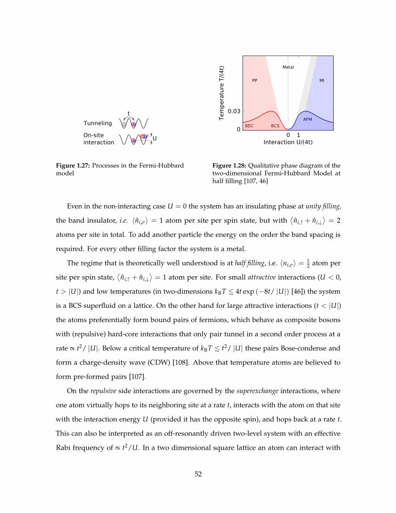
t
Tunneling
UOn-siteinteraction
Figure 1.27: Processes in the Fermi-Hubbardmodel
Tem
pera
ture
1T/(
4t)
Interaction1U/(4t)0
0
AFM
BEC BCS
Metal
0.03
MIPP
1
Figure 1.28: Qualitative phase diagram of thetwo-dimensional Fermi-Hubbard Model athalf filling [107, 46]
Even in the non-interacting case U = 0 the system has an insulating phase at unity filling,
the band insulator, i.e. 〈ni,σ〉 = 1 atom per site per spin state, but with⟨ni,↑ + ni,↓
⟩= 2
atoms per site in total. To add another particle the energy on the order the band spacing is
required. For every other filling factor the system is a metal.
The regime that is theoretically well understood is at half filling, i.e. 〈ni,σ〉 = 12 atom per
site per spin state,⟨ni,↑ + ni,↓
⟩= 1 atom per site. For small attractive interactions (U < 0,
t > |U|) and low temperatures (in two-dimensions kBT > 4t exp (−8t/ |U|) [46]) the system
is a BCS superfluid on a lattice. On the other hand for large attractive interactions (t < |U|)
the atoms preferentially form bound pairs of fermions, which behave as composite bosons
with (repulsive) hard-core interactions that only pair tunnel in a second order process at a
rate ∝ t2/ |U|. Below a critical temperature of kBT > t2/ |U| these pairs Bose-condense and
form a charge-density wave (CDW) [108]. Above that temperature atoms are believed to
form pre-formed pairs [107].
On the repulsive side interactions are governed by the superexchange interactions, where
one atom virtually hops to its neighboring site at a rate t, interacts with the atom on that site
with the interaction energy U (provided it has the opposite spin), and hops back at a rate t.
This can also be interpreted as an off-resonantly driven two-level system with an effective
Rabi frequency of ∝ t2/U. In a two dimensional square lattice an atom can interact with
52

Band insulator
Bound paircondensate
Metal
Anti-ferromagnet
Mott insulator
Atom number
Tem
pera
ture
(U > 0) Interactions (U < 0)
Figure 1.29: Various phases of the Fermi-Hubbard model
its 2d = 4 nearest neighbors. Strong interactions t > U are going to drive the system into
a Mott insulator with one atom per site. This has experimentally been first studied in the
groups of Tilman Esslinger [109] and Immanuel Bloch [110]. For low enough temperatures
(T < TNeel, see [111]) the Mott insulator is going to exhibit spin ordering as well and form
an anti-ferromagnet with a checker-board pattern, which has yet to be demonstrated in an
optical lattice experiment. Several groups are working on detection schemes that do not
rely on single-site imaging [112, 50]. As mentioned in the introductory chapter the main
experimental focus is on the repulsive Fermi Hubbard model, as it may exhibit a d-wave
superfluidic phase for hole-doped samples [49].
Mathy and Huse [111] also predict a phase separated ferro-magnetic phase for strong
interactions in shallow lattices, where the direct nearest-neighbor interaction caused by the
Wannier function overlap between neighboring lattice sites favors same spins on neighboring
sites. This is one example of an effect that could be observed in our experiment and that
goes beyond the Fermi-Hubbard description with only on-site interactions.
1.5.4.1 Spin Mapping: The Heisenberg Model
At half-filling and at low temperatures (T < t2/U) the atoms in the repulsive Fermi Hubbard
model can be also understood as localized spins, that only interact via the superexchange
interaction J = 4t2/U. The spin model is a convenient picture for quantum information
processing. For fermions this gives rise to an isotropic anti-ferromagnetic Heisenberg (XXX)
53

Hamiltonian [113]
HJ = J ∑〈i,j〉
Si · Sj, (1.139)
with the spin-1/2 operator in site i Si =12
(σx, σy, σz
)and the Pauli spin matrices σi.
This mapping can be easily seen for two-fermions (↑, ↓) in a double well (L, R):
H(2)FH = −t
(c†
L,↑ cR,↑ + c†R,↑ cL,↑ + c†
L,↓ cR,↓ + c†R,↓ cL,↓
)+ U
(nL,↑nL,↓ + nL,↑nL,↓
). (1.140)
The ground state for t = 0 and U > 0 is given by |ψ0〉 = (|↑, ↓〉 − |↓, ↑〉) /√
2. For now let us
just consider the |↑, ↓〉 component. Finite tunneling admixes the excited states |↑↓, 0〉 , |0, ↑↓〉.
In second order perturbation theory [81] in t the energy shift is given by
∆E = t2 ∑|ψ〉,|ψ′〉
∣∣∣⟨ψ′∣∣∣ c†
L,↑ cR,↑ + c†R,↑ cL,↑ + c†
L,↓ cR,↓ + c†R,↓ cL,↓
∣∣∣ψ⟩∣∣∣2⟨
ψ∣∣ HFH(t = 0)
∣∣ψ⟩−⟨ψ′∣∣ HFH(t = 0)
∣∣ψ′⟩ = −2t2
U(1.141)
For two identical spins (|↑, ↑〉 or |↓, ↓〉) in the double well there is no shift due to the
Pauli exclusion principle. Comparing this two the energies of the two-site Heisenberg model
H(2)J = JSL · SR (1.142)
and ignoring the constant energy offset we obtain
J = 4t2
U. (1.143)
54

Chapter 2
Raman Cooling
In the early days of Bose-Einstein condensation it was attempted to laser-cool below the
condensation temperature. Under typical conditions for ultracold dilute quantum gases the
transition temperature is TBEC ∼ O(100 nK). Typical Doppler-cooling techniques are limited
to the Doppler temperature (3.13) which for the alkali atoms is TD = hγkB2 ∼ O(100µK).
Sub-Doppler cooling techniques like polarization gradient cooling [114] in turn is only
limited by the recoil energy of the cooling photons: Tr =h2k2
2mkB∼ O(1µK) [115], still above
the transition temperature. A promising candidate for sub-recoil cooling is the so called
motional sideband cooling, where one explicitly drives transitions between resolved vibrational
levels in a trap. Although pure laser-cooling to quantum degeneracy of alkali atoms1 has
not been achieved in neutral atoms, sideband cooling is the standard technique to cool
trapped ions to their vibrational ground state [117].
2.1 Vibrational Transitions
For sideband cooling we need to treat the motion of a trapped atom quantum-mechanically.
In the derivation of the driven two-level system (1.1.2.1) we neglected the motion of the
atom by approximating exp (ik · r) ≈ 1. This assumption becomes invalid once the extent
1Recently Stellmar et al. [116] have laser-cooled the alkaline-earth atom 84Sr to degeneracy via narrow-lineDoppler cooling.
55

of the wavefunction is on the order of the optical wavelength. For simplicity let us assume
that an atom is trapped in a harmonic trap (1.3) in the resolved sideband regime, where the
trap frequency ω is larger than the natural linewidth of the optical transition γ ω and
the Rabi frequency Ω ω. Its wavefunction then is a product of the electronic state |i〉 and
motional state |ν〉
|ψ〉 = |i〉 |ν〉 ≡ |i, ν〉 . (2.1)
The frequency of the driving field is chosen such that it is resonant with the |1, ν〉 to
|2, ν′〉 transition, i.e. ωL = ωA + ω(ν′ − ν). Taking the vibrational states into account the
transition matrix element is given by
⟨2, ν′
∣∣∣ dE∗ exp (−ik · r)∣∣∣ 1, ν
⟩= hΩ0
⟨ν′∣∣ exp (−ik · r)
∣∣ ν⟩= hΩ0µν′,ν, (2.2)
with the free space Rabi frequency Ω0 (1.13).
For a single beam and an isotropic trap we can assume that k is along the x-direction.
Using the ladder operator formalism (1.39) we can rewrite the motional part of the matrix
element as
µν′,ν =⟨
ν′∣∣∣ exp
(−iη
(a + a†
)) ∣∣∣ v⟩
, (2.3)
with the Lamb-Dicke parameter
η =1√2
kaQHO =
√Er
hω. (2.4)
The definition of recoil energy Er =h2k2
2m is identical to the recoil energy in an optical lattice
(see 1.5.1.2 for example), but the wavelength is the resonant atomic wavelength (671 nm), not
the lattice wavelength (1064 nm)! In our experiment with a trap frequency of about 1 MHz
the Lamb-Dicke-parameter is on the order of η∼0.27.
The total Rabi frequency can be calculated analytically [118]
Ων′,ν = Ω0 exp(−η2
2
)(iη)|ν
′−ν|
√ν<!ν>!
L|ν′−ν|
ν< (η2), (2.5)
where ν< (ν>) is the level of the lower (higher) excited state and Lαn(x) are nth-order
56
generalized Laguerre polynomials [82]. But it is more instructive to only look at the leading
order term for η 1. For example the transition from |ν = 0〉 to |ν′ = 1〉 has a matrix
element µ(1)1,0 = −iη. The transition |ν〉 to |ν′ = ν + 1〉 has an enhanced amplitude due to
the Bose enhancement of
µ(1)ν+1,ν = −i
√ν + 1η. (2.6)
Transitions spanning two vibrational levels are based on a higher order process. Therefore
the transition matrix element is reduced by another order in η
µ(2)ν+2,ν = −1
2
√(ν + 2)!
ν!η2.
Transitions to a lower vibrational level are called the red sideband, to a higher vibrational
level the blue sideband. The transition frequency that does not change the vibrational state is
called the carrier.
On the one hand being deeper in the Lamb-Dicke regime (η 1) means that it gets
harder to drive transitions between motional states, but on the other hand it is less likely
to change the vibrational state during a spontaneous emission event! As pointed out by
Kerman [119] this does not mean that recoil heating is suppressed. In free space the kinetic
energy of an atom at rest increases by Er, when it spontaneously emits a photon. If the
spontaneous emission happens inside a tight trap the probability to change into an excited
state is ≈ η2, but when it does its energy increases by hω = Er/η2 > Er, so that on average
the energy increase again is Er.
2.2 Raman Transitions
In typical experiments with neutral alkali atoms the linewidth γ (∼2π · 6 MHz) is much
larger than the trap frequency ω (∼2π · 1 MHz). Hence it is not possible to directly resolve
the motional sidebands with a single laser. By using a two-photon scheme the effective
linewidth can be made (almost) arbitrarily narrow, so that the sidebands can be resolved
nevertheless.
57

ωL+Ω'
ωL-Ω'
ωL
ωL
Ω'δ
Figure 2.1: Spontaneous emission in thedressed-atom model
−1 0 1
0
10
20
30
Fluor. freq. (ωF−ω0)/Ω
ScatteringRate
γsc
/Ω
Figure 2.2: Resonance fluorescence spectrumof a strongly-driven two-level system (γ =Ω/10, δ = 0). The coherent peak is displayedwith a device resolution of ∆νmeasurement =Ω/100. atom
A three-level system in a Λ configuration is described by the Hamiltonian in the rotating-
wave approximation [58] (see (1.12))
H = −hδ13 |3〉 〈3| − hδ2 |2〉 〈2| −h2(Ω13 |3〉 〈1|+ Ω23 |3〉 〈2|+ h.c.) , (2.7)
where Ω13,23 denote the coupling between the groundstates |1〉 , |2〉 and the excited state |3〉,
δi3 the detuning of the laser ωL,i3 from the resonance ωA,i3, and the two-photon detuning
δ2 = δ23 − δ13. (2.8)
In the limit where |1〉 and |2〉 are almost degenerate δ23 ≈ δ13 = δ and the laser is far
detuned from the excited state |3〉, the excited state can be adiabatically eliminated and the
problem reduces to a two-level system with an effective two-photon Rabi frequency
Ω2 =Ω∗23Ω13
4δ. (2.9)
58

2.3 Optical Pumping: Coherent Vs. Incoherent Scattering
Using the dressed-atom picture [120] we can quickly gain some intuition about the spectrum
of the light scattered by a single two-level atom. The dressed-atom model assumes a
quantized driving electromagnetic field with the Hamiltonian
HL = hωL
(n +
12
). (2.10)
The coupling of an atom to the light field with n photons mixes the ground and excited
states |1, n〉 , |2, n′〉 for photon numbers differing by 1. In the weak driving limit the states
are given by
|+, n〉 ≈ |2, n〉+ ε |1, n + 1〉 (2.11)
|−, n〉 ≈ |1, n + 1〉 − ε |2, n〉 ,
with the energies
E±,n = hωL(n +12) +
hδ
2± hΩ′
2. (2.12)
The dressed states are split by the generalized Rabi frequency (1.15) Ω′ =√
Ω2 + δ2 =
δ + Ω2
2δ +O(Ω4) (see figure 2.1). Spontaneous emission couples the bare states |2〉 → |1〉.
Hence there exist four transitions with three distinct frequencies ωL, ωL −Ω′, and ωL + Ω′
for the decay between the n and n− 1 manifold. The whole spectrum is composed of a
elastic (coherent) δ-like peak at the laser frequency ωL and inelastic (incoherent) peaks with
widths on the order of the natural linewidth γ. In the limit of strong driving Ω′ γ the
three incoherent peaks give rise to the Mollow triplet [121, 122] (also see figure 2.2).
The full fluorescence spectrum can be obtained solving the Master equation (see, for
example, Scully and Zubairy [59]). The ratio of incoherently to coherently scattered total
intensity is given by [121]Iincoherent
Icoherent= 2
Ω2
γ2 + (2δ)2 . (2.13)
The inelastic/incoherent part is uniformly scattered into the whole 4π solid angle, whereas
the elastic/coherent emission pattern depends on the incident polarization and the atomic
59

structure of the scattering atom [123].
For multiple atoms in an optical lattice the coherent nature of the elastically scattered
light produces sharp interference features, Bragg peaks, which can be seen in the far-field or
in the Fourier plane of an imaging system. Some groups use this as a technique to study
the ordering in the lattice without single-site imaging [50, 112]. Bragg scattering has also
been observed with a quantum gas microscope [124]. The angles under which the nth-order
peak appear are given by [124]
sin θn = 1 +λ
dlat, (2.14)
where the periodicity of the lattice is given by dlat and the atoms are coherently scattering
light of the wavelength λ. Only one peak is captured by the imaging system of our
experiment. Since the Bragg peak is narrow in Fourier space it contributes to a smooth
background in the image plane.
Even for a single two-level atom (with only a single cycling transition) coherent scattering
dominates for weak drive, but in a multi-level system coherent Raman-like transitions to
non-degenerate ground state levels wash out the interference between multiple scattering
for observation times longer than the inverse level spacing [123]. The transitions can be
understood as a Raman transition, where the down leg is stimulated by a vacuum photon
in a similar fashion as for normal elastic scattering.
2.4 Raman Sideband Cooling In A Bias Field
Commonly Raman cooling uses a magnetic field to break the degeneracy of the magnetic
sublevels in the ground state [125, 126, 127, 128, 129]. In the case of degenerate sideband
cooling the Zeeman magnetic field is tuned to bring |ν〉 and |ν− 1〉 of different magnetic
sublevels into resonance (µB = hωtrap). Conceptually even easier is the case where one uses
two phase-coherent laser beams that are detuned such that the Raman transition covers the
Zeeman splitting and the vibrational splitting for the |ν〉 → |ν− 1〉 transition. One needs
to ensure that the Stark shift of the Raman lasers, i.e. the two-photon Rabi frequency, is
60

22S1/2
22P1/2
mF=-3/2 mF=-
1/2 mF=1/2 mF=
3/2
F=1/2
F=3/2
F=1/2
F=3/2
(σ+ )
Ram
an(σ+ )
Pump
(π)
Raman
Figure 2.3: Raman sideband cooling scheme for 63Li using a bias magnetic field to Zeeman-shift the
magnetic sublevels
smaller than the Zeeman splitting.
Our scheme for 6Li is depicted in figure 2.3. Here the two Raman beams are 7 GHz
red-detuned of the D1 transition and couple the |6, ν〉 =∣∣22S1/2(F = 3
2 , mF = 32 )⟩|ν〉 to the
|5, ν− 1〉 =∣∣22S1/2(F = 3
2 , mF = 12 )⟩|ν− 1〉 state. The optical pumping laser then brings the
atoms back into the initial electronic state, while preserving the vibrational state |5, ν− 1〉 →
|6, ν− 1〉. The probability of decay into a different vibrational state is suppressed by the
Lamb-Dicke parameter η. The scattered photon plays an important role in our imaging
process (see 2.9). With the given choice of polarizations the |6〉 state is dark for the pumping
beam limited only by the purity of the polarization.
Because of the unfavorable branching ratios an additional repumping beam is neces-
sary to bring the atoms back from the∣∣22S1/2(F = 1
2 )⟩
manifold into the∣∣22S1/2(F = 3
2 )⟩
manifold. This is achieved with a weak laser resonant with the∣∣22S1/2(F = 1
2 )⟩
to∣∣22P3/2
⟩transition.
Although the∣∣22S1/2(F = 3
2 )⟩
manifold is not a closed two-level system, we were able to
observe Rabi oscillations between the |6〉 and |5〉 state, but the revival is not perfect because
of the coupling to the |4〉 and |3〉 states. From the timescale of the depletion of the |6〉 state
we estimate our two-photon Rabi frequency to be Ω2 ∼ 20 kHz on the carrier transition
61

0 100 200 300
1
2
3
·104
Time t (µs)Atomsin
| 6⟩(a.u.)
Figure 2.4: Rabi-like oscillations in the driven four-level system |3 . . . 6〉
(∆ν = 0) for laser power of .
From a cooling perspective any of the |4〉, |5〉, |6〉 states is suitable for a Raman transition
that takes out a vibrational quanta. So in principle even under imperfect optical pumping
the cooling can still work, except that an atom needs to scatter multiple until it is pumped
into the dark state. A Raman spectrum taken with a bias field of B ∼ 150 mG can be seen in
figure 2.5. Here the atoms were first optically pumped into the |6〉 state and the driven into
the |5〉 state via the Raman transition.
2.5 Three-Dimensional Cooling
To cool all three motional degrees of freedom one needs to make all the trap frequencies
degenerate or address all trap frequencies individually, one at a time. In our experiment
the two-photon detuning is sequentially tuned onto the red sideband of the radial and
axial lattices and then swept over the width of the resonance features to allow for spatial
inhomogeneity in the trap frequencies (see figure 2.5).
In addition to tuning to the correct frequency, there needs to be momentum transfer
along the direction one attempts to cool. This can be seen from the x · k term in the
vibrational coupling (2.2). If x and k are not aligned, the Lamb-Dicke parameter (2.4) is
reduced by |cos θ|, where θ is the angle between the two vectors. For a two-photon transition
62

−2.5 −2 −1.5 −1 −0.5 0 0.5 1 1.5 2
0
0.5
1
carrier — heating —— cooling —
vertical
NE
NW
vertical
NE
NW
Detuning (MHz)
Remainingatomsin
| 6⟩
Figure 2.5: Raman spectrum taken by driving |6〉 → |5〉 at a bias field of 150 µG
the effective momentum kick k that the atom experiences from absorption (k1) followed by
stimulated emission (−k2) is
k = k1 − k2. (2.15)
To maximize the coupling to all three lattice axes with a single pair of Raman beams one
needs to choose k such that it spans a 45 angle with all the lattice axes. Due to space
constraints in our experiment the angle between the direction of the momentum transfer
and the vertical lattice (z) is only ∼75 so that the coupling is reduced by a factor of 25%.
The coupling to the radial lattice axes is only reduced by 1/√
2.
2.6 Alignment
Since the |6〉 state is dark for the optical pumping, the polarization of the optical pumping
can easily be optimized by maximizing the lifetime in the stretched state. The |6〉 state can
be prepared with a microwave sweep driving the |1〉 → |6〉 transition. When completely
optimized we can achieve a ratio of the lifetimes for the two circular polarizations of
τσ+
τσ−∼ 10 . . . 100. (2.16)
All polarization assume a certain quantization axis set by the magnetic bias field. The
63

0 5 10 15
0
20
40
Time t (ms)
Atomsin
| 6⟩(a.u.)
pol. misaligned
0 500 1,000
Time t (ms)
pol. aligned
Figure 2.6: Decay out of |6〉 while exposed to optical pumping light with and without optimizedpolarization
direction of the magnetic field has to be optimized as well, so that it points along the
σ+-Raman and optical pumping beam. The wrong circular polarization can in principle
drive a wrong sideband (i.e. a blue sideband), but that transition is detuned by the Zeeman
shift and thus suppressed.
The polarization of the linearly polarized π-Raman beam is set to minimize the reflection
off the glass cell. This procedure is roughly equivalent to setting the polarization to be
vertical (along z). The polarization of the σ+-Raman beam is optimized by transferring
population out of the |6〉 state via the carrier Raman transition.
The pointing for all the Raman and optical pumping beams is optimized by heating
trapped atoms out of the lattice with one beam at a time. For the fine alignment the beams
need to be attenuated further with neutral density filters.
2.7 Raman Sideband Cooling At Zero Field
The problem of the finite “darkness” of the |6〉 state due to imperfect polarizations can be
avoided by altering the cooling scheme and working at negligible bias field (µBB hΩ2
ωtrap). Without the Zeeman field all the magnetic sublevels are degenerate and we can
drive Raman transitions between the∣∣22S1/2(F = 3
2 )⟩
and∣∣22S1/2(F = 1
2 )⟩
manifold while
tuning to the red sideband. An optical pumping beam pumps the atoms back into the
64

22S1/2
22P1/2F=1/2
F=3/2
Raman
Pump
F=3/2
F=1/2
Figure 2.7: Raman sideband cooling scheme for 63Li without a bias field
∣∣22S1/2(F = 32 )⟩
manifold. The upper manifold is 228 MHz detuned from the pumping light
so that the scattering rate (1.30) is suppressed by ≈ Ω2/δ2 ∼ O(10−4) (for a s0 = 0.1). The
Raman spectrum acquired in the B = 0 configuration is given in figure 2.8. Without the bias
field the carrier is exactly at zero detuning. Within the noise there are no transitions on the
cooling sidebands. This is a strong indication that the atoms are in the lowest band of our
optical lattice.
2.8 Heating Mechanisms
During the cooling atoms in the optical lattice are subject to several heating mechanisms.
The most severe one is the loss of pairs of atoms due to light-assisted collisions [130]2. The
potential curves for scattering of a∣∣22S1/2
⟩ground state atom with an excited state
∣∣22P1/2⟩
are altered by the long range dipole interaction. In case of red-detuned (blue-detuned) light
the atoms experience a long range attractive (repulsive) interaction ∝ 1/r3. Atoms can either
end in a bound-state (photoassociation) with the photon carrying away the excess energy
or the excess energy is released as kinetic energy after the excited state decays back to the
ground state. Due to the repulsive nature of the interaction for blue-detuned light inelastic
2In the context of magneto-optical traps light-assisted collisions are also called radiative escape [131]
65

−2.5 −2 −1.5 −1 −0.5 0 0.5 1 1.5 2
0
0.5
1
carrier — heating —— cooling —
vertical
NE
NW
vertical
NE
NW
Detuning (MHz)
Remainingatomsin
∣ ∣ ∣22S1
/2,F
=1 /2⟩
Figure 2.8: Raman spectrum taken by driving atoms into the∣∣22S, F = 3/2
⟩manifold with a single
sweep over ±50 kHz in 500 µs
processes are suppressed [130].
Additionally mixtures of different magnetic sublevels of the two groundstate manifolds∣∣22S1/2(F = 32 )⟩
and∣∣22S1/2(F = 1
2 )⟩
can release energy on the order of the hyperfine
splitting via spin-changing collisions. This effect together with the light-assisted collisions
makes it impossible to have two atoms tightly confined to a single lattice site while scattering
resonant photons, which will most likely result in parity imaging, where one can only detect
the atom number per site modulo two [35]
For a single atom on a lattice site the following other heating mechanisms remain. Single
photon scattering imparts the photon momentum onto the atom it scatters of. In the case of
an atom at rest its energy increases by up to 2Er and 1Er on average for incoherent scattering.
This recoil heating can occur both for optical pumping and the Raman beams. Because of
the small fine structure of 6Li of only 10 GHz the optimum detuning of the Raman beam
coupling different magnetic sublevels is on that order [132]. In this regime the ratio of single
photon scattering rate to two-photon Rabi frequency is on the order of 1/100.
In addition, atoms in an excited state experience a different trapping potential due
to its different polarizability. For cooling of 6Li on the 2s to 2p transitions in a trap at
1064 nm luckily this effect is rather small. The polarizability of the ground state∣∣22S1/2
⟩is α2s = 271 au, for
∣∣22P1/2⟩
α2p,D1 = 202 au, for∣∣22P3/2(mF =
∣∣ 12
∣∣)⟩ α2p,D2,1/2 = 221 au, and
66

for∣∣22P3/2(mF =
∣∣ 32
∣∣)⟩ α2p,D2,3/2 = 183 au, where the atomic polarizability unit is defined as
au = 4πε0a30 [60].
A classical estimation for the fluctuating dipole force heating/stochastic heating is given
in [100]. Taking the finite excited state decay rate γ into account the fractional energy
increase per excitation is given by
ε =E3 − E1
E1=
(ω2
1 −ω22)2
ω21
(γ2 + 4ω2
2
) . (2.17)
For 6Li atoms in a 1064 nm lattice with a ground state trap frequency of ω1 = 2π · 1 MHz
subject to D1 cooling light this results in a fractional energy increase of ε = 0.0018 per
excitation. Assuming that the initial energy E1 is on the order of hω1 ≈ 13.5E(671 nm)r the
energy gain is only 0.024 times the resonant photon recoil energy of E(671 nm)r = h · 73.9 kHz.
Besides choosing a (near-)magic wavelength for the optical trap, this kind of heating can
also be minimized by keeping the saturation parameter low, so that there is negligible
population in the excited state. While this kind of heating has little effect for cooling on the
D1,2 transitions, it could be a problem, for example, if one would want to directly resolve
the vibrational sidebands by using the narrow ultraviolet 2s to 3p transition. Although there
is a magic wavelength near 1070 nm, the 3p state decays predominantly via the 3s state as
intermediate state which has large polarizability with opposite sign [100].
As for all optical traps technical noise, like residual amplitude modulation, can cause
parametric heating as well (see 1.4.4). This becomes especially problematic during the imaging
when the lattice depth is maximal with high trap frequencies, since heating rates scale
super-linearly with the trap frequency (ωα, α ≥ 2).
2.9 Raman Imaging
We would like to use the scattered photons of the optical pumping process for fluorescence
imaging. Because of the second order nature of the Raman process, we are going to need
significantly higher laser powers for the Raman transitions than for the optical pumping.
For a 100µs long Raman pulse with 1 mW and a hypothetical uniform intensity over
67

GateOn
Off
Ramanfrequency
& amplitude
Pumping
Time ttpump
tRaman
On
Off
f1
f2
f3
f4
Figure 2.9: Gated imaging during the Raman cooling
100× 100 lattice sites the atoms are illuminated with 3× 10¹¹ photons at 671 nm in total.
If we assume we only see Rayleigh scatter on the order of 10 ppm off the superpolished
substrate, 3× 10⁶ photons get scattered in total and 300 photons per lattice site. During
the optical pumping pulse each atom only scatters O(1) photons before it gets optically
pumped into a dark-state. This scenario would result in a signal-to-noise ratio of ∼1 : 100,
which is far from being enough to resolve individual atoms (for a rather low overall count
rate).
2.9.1 Pulsed Raman Imaging
Due to the small fine-structure splitting of only 10 GHz it is virtually impossible to spectro-
scopically filter the cooling light from the imaging light with, for example, a dichroic mirror.
Instead of trying to separate the light spectroscopically, we are separating the Raman from
the pumping light temporally by performing up to 6000 two-step cooling processes and
only exposing the camera during the optical pump pulse.
For the initial tests with the low-resolution imaging we used a mechanical chopper
(Thorlabs MC2000 with MC1F30 blade) in the intermediate imaging plane (see figure 3.18)
to block the camera during the Raman pulses. The rotation of the chopper is phase-locked
to the experiment with the blades opening and closing at 2 kHz.
Because of the finite aperture of the chopper blades, it is not possible to use this setup in
the high resolution imaging described in section 3.3.1.5. It might be possible to create an
intermediate demagnified image with another long working distance microscope objective,
68
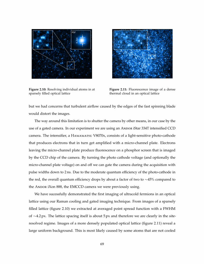
PSF
4.2px
Figure 2.10: Resolving individual atoms in atsparsely filled optical lattice
Figure 2.11: Fluorescence image of a densethermal cloud in an optical lattice
but we had concerns that turbulent airflow caused by the edges of the fast spinning blade
would distort the images.
The way around this limitation is to shutter the camera by other means, in our case by the
use of a gated camera. In our experiment we are using an Andor iStar 334T intensified CCD
camera. The intensifier, a Hamamatsu V8070x, consists of a light-sensitive photo-cathode
that produces electrons that in turn get amplified with a micro-channel plate. Electrons
leaving the micro-channel plate produce fluorescence on a phosphor screen that is imaged
by the CCD chip of the camera. By turning the photo cathode voltage (and optionally the
micro-channel plate voltage) on and off we can gate the camera during the acquisition with
pulse widths down to 2 ns. Due to the moderate quantum efficiency of the photo-cathode in
the red, the overall quantum efficiency drops by about a factor of two to ∼45% compared to
the Andor iXon 888, the EMCCD camera we were previously using.
We have sucessfully demonstrated the first imaging of ultracold fermions in an optical
lattice using our Raman cooling and gated imaging technique. From images of a sparsely
filled lattice (figure 2.10) we extracted at averaged point spread function with a FWHM
of ∼4.2 px. The lattice spacing itself is about 5 px and therefore we are clearly in the site-
resolved regime. Images of a more densely populated optical lattice (figure 2.11) reveal a
large uniform background. This is most likely caused by some atoms that are not cooled
69

enough and tunnel during the imaging process. An additional effect could be the Bragg
scattering for denser clouds (see 2.3) that is expected to produce a smooth background
as well. But these shortcomings are being addressed right now, while this work is being
written.
2.9.2 Fidelity: Imaging A 3× 3 Plaquette Or Single Atom Minesweeper
In this section I want to demonstrate the effect of overlapping point spread functions
when imaging single atoms in an optical lattice. As a model I am going to use a 3× 3
plaquette with variable filling factor and focus on the central lattice site. The particles are
non-interacting with a maximum occupation of one per site. This would be valid model for
a spin polarized Fermi gas in the ground band of an optical lattice or one spin state of a
non-interacting multi-component Fermi gas. Effects like electronic noise or photon counting
statistics will be ignored here. It is assumed that the fluorescence image gets analyzed by
integrating up the fluorescence of each lattice site.
The nine lattice sites are labeled with the following indices
8 1 5
4 0 2
7 3 6
. (2.18)
Using those indices we can write all 29 = 512 possible states encoded as a binary number,
for example
|0000000002〉 = , |0000000012〉 = , |0000000102〉 = ,
|1010100112〉 = |1111111102〉 = |1111111112〉 = .
The sites can be grouped into three categories: the center site 0, the nearest neighbors
1, 2, 3, 4, and the next-nearest neighbors 5, 6, 7, 8. Atoms in each category are going to have a
different contribution of their point spread function to the total intensity in the square of
70

0 1 2
0
0.2
0.4
0.6
Resolving power αWeight
w04wnn4wnnn
Figure 2.12: Contribution to the fluorescence on the center site from nearest neighbors and next-nearest neighbors
site 0. For simplicity the point spread function is approximated as a Gaussian of the form
psf(x, y) =1
πs2 exp(− x2 + y2
s2
). (2.19)
With that we can get analytic expressions for the “leakage” of the point spread function
onto the center site from the nearest and next-nearest neighbors wnn, wnnn (see figure 2.12):
w0 =∫ αs/2
−αs/2dx∫ αs/2
−αs/2dy psf(x, y) = erf2
(12
α
)(2.20)
wnn =∫ 3αs/2
αs/2dx∫ αs/2
−αs/2dy psf(x, y) =
12
erf(
12
α
)(erf(
32
α
)− erf
(12
α
))wnnn =
∫ 3αs/2
αs/2dx∫ 3αs/2
αs/2dy psf(x, y) =
14
(erf(
32
α
)− erf
(12
α
))2
.
Here the lattice spacing is assumed to be αs. The total probability to collect fluorescence
from the center site for any state can be written as
w(n0, nnnnnnn) = n0w0 + nnnwnn + nnnnwnnn,
with n0 ∈ 0, 1 atoms on the center site, nnn ∈ 0, 1, . . . , 4 on the nearest neighbor sites, and
nnnn ∈ 0, 1, . . . , 4 on the next-nearest neighbor sites. In total there are 2 · 5 · 5 = 50 different
values for fluorescence level w, but some of these stem from different states/configurations.
For example , , , , ,and will have identical fluorescence. In general each w is
( 2n0)( 4
nnn)( 4
nnnn) fold degenerate.
71

0 0.5 1
0
0.05
0.1
Fluorescence w(n0,nnn,nnnn)
Probability
p0 = 0.3,α= 1.6
0 0.5 1
Fluorescence w(n0,nnn,nnnn)
p0 = 0.3,α= 1.0
n0 = 0n0 = 1
Figure 2.13: Total fluorescence in the central lattice site for different optical resolutions
The probability to find an atom on a given site is denoted by p0. If the 3× 3 plaquette is
considered to be part of a larger system, p0 can also be interpreted as the filling factor. The
probability to find the plaquette in a given state/configuration with n = n0 + nnn + nnnn
atoms is given by
pn = pn0(1− p0)
9−n. (2.21)
Combining all this we find that the probability to get w(n, nnn, nnnn) is
p (w(n0, nnn, nnnn)) =
(2n0
)(4
nnn
)(4
nnnn
)pn0+nnn+nnnn
0 (1− p0)9−n0−nnn−nnnn . (2.22)
The distribution is visualized for a sparse lattice in figure 2.13.
The fidelity of the imaging (with this particular way of analyzing the images) depends
on whether we can distinguish configurations with a hole in center from the ones with
an atom . For realistic parameters the worst case is trying to separate and . The two
fluorescence levels w(0, 4, 4) and w(1, 0, 0) can be resolved for
α > α0 ≈ 1.48. (2.23)
Around this point the “fidelity” defined as F = 12 (w(1, 0, 0)− w(0, 4, 4) + 1) scales linearly
with the resolving power α
F(α) =12(w(1, 0, 0)−w(0, 4, 4)+ 1) ≈ 0.500+ 0.447(α− α0)− 0.025(α− α0)
2 +O((α− α0)3).
72

Raw β= 0.5 β= 1.0 β= 1.5 β= 2.0
t= 0.10s t= 0.25s t= 0.50s t= 1.00s
Figure 2.14: Simulation of fluorescence imaging for a scattering rate of 3 kHz
This limit can be circumvented by using more an advanced analysis algorithm that takes
the surrounding lattice sites into account instead of looking at each site individually and I
would like to emphasize that the model described in this section does not take the actual
photon detection including counting uncertainty and noise into account.
2.9.3 Monte-Carlo Imaging Simulation
To get a feel for how fluorescence images are going to look as a function the imaging
parameters, like resolution, exposure time, noise, etc. it is helpful to simulate the imaging
process. I have done this as a Monte-Carlo simulation, where for every small time interval
∆t the following probabilities are calculated for each site: probability that the atom is lost
(loss rate), has scattered a photon (scattering rate), and the scattered photon is detected
(numerical aperture, quantum efficiency of sensor, transmission of optical setup). Each
detected photon is added to the sensor with a Gaussian probability distribution centered
on the originating lattice site. This is emulating the point spread function of the imaging
setup. In addition, dark-counts get added to the sensor each time step. At the end of the
simulation readout noise is added to the sensor following a normal distribution.
With this (admittedly brute-force) Monte-Carlo approach one can already study the
effect of dark-counts, scattering rate, and resolution to determine parameters that would
73

allow imaging with sufficient fidelity. Figure 2.14 shows simulated images for a filling factor
of p0 = 0.5 and varying spot sizes β (with t = 0.5 s) and exposure times t (with β = 1). The
standard deviation of the point spread function is β/2 times the lattice spacing.
74

Chapter 3
Experimental Setup
3.1 Vacuum System
Besides the atomic beam source and pumping sections the experiment consists of two
connected vacuum chambers, the main chamber and the science chamber (3.1). This two-
chamber design has the advantage that there is not direct line-of-sight to the hot source,
which could potentially reduce the trap lifetime. In addition, the secondary chamber can be
swapped out relatively easy to accommodate different very specialized setups.
In the former, slow atoms from the Zeeman slower (see section 3.4.2) get captured and
cooled in a magneto-optical trap (see section 3.4.3). With the aid of a high power optical
dipole trap (3.3.7) and magnetic field coils [100] that allow to increase the interparticle
scattering cross section by the use of a Feshbach resonance (1.2), the atoms can be cooled
further, even to a point where the lithium atoms condense into a molecular Bose-Einstein
condensate (3.36). This is an ideal starting point to perform cutting edge experiments with
the ultracold atoms.
Because a quantum gas microscope (3.3.1) requires a large amount of optical access,
the science chamber is a fused silica glass cuvette (3.1.2). Additionally using glass avoids
eddy currents caused by switching magnetic fields and changing magnetic fields due to
magnetizable materials.
75

glass cellion pump titaniumsublimation
titaniumsublimation
titaniumsublimation
ion pump
mainchamber
ion pumps
differential pumping
section
oven section
Zeeman slower
Figure 3.1: Overview of the vacuum chamber
To achieve a low background pressure in the science chamber, it is pumped by the com-
bination of a GammaVacuum TiTan DIX 75S diode-style ion pump and a GammaVacuum
titanium sublimation pump connected via an intermediate pumping chamber. A large gas
load in a glass cell comes from helium diffusion through the glass. A differential diode-style
ion pump is more efficient at pumping noble gasses (He, Ar, ...) than the typical diode
pumps while sacrificing a little in overall pumping speed [133].
In addition to the ion pump, the titanium sublimation pump is helps pumping the
remaining reactive gasses (CO, CO2, O2, etc.) in the system and to some extent even
hydrogen H2 [133]. After degassing during the bake out, each of its filaments has been fired
multiple times for 1 min at a current of 48 A to sputter titanium onto the walls of the pump
chamber. To avoid shorting the ion pump cells the pump chamber has a smooth 45 before
it attaches to the pump. In this configuration there is no direct line-of-sight between the ion
pump and the titanium filaments.
We found that ion gauges significantly contribute to the gas load. Therefore the pressure
is only measured at a single point of the experiment, reading 3 · 10−12 torr. This number is
consistent with the lifetimes measured in the main chamber.
During the bake-out we had a residual gas analyzer (RGA) attached to the chamber (on
the UHV side of the pump). The idea was to more accurately measure the pressure once
the chamber has been sealed of from the turbo pump, but it turned out that, although the
76

Figure 3.2: Drawing of the main chamber
RGA had been baked as well, turning it on released so much gas that the chamber had to be
rebaked (probably electron desorption). For future bake-outs I would recommend to only
use the RGA either continuously during bake-out or, even better, only on the rough vacuum
side.
3.1.1 Main Chamber
The main chamber (figure 3.2) is a custom octagonal vacuum chamber made from 316-series
stainless steel manufactured by Sharon Vacuum. It has ports for the magneto-optical
trapping beams, the high-power optical dipole trap, and two electric feed-throughs for
microwave antennae. For a more detailed description see my diploma thesis [134].
3.1.2 Glass Cell
The rectangular cuvette (figure 3.3) of the dimensions 45 mm× 35 mm× 110 mm with 5 mm
walls was manufactured by Japan Cell and distributed by Triad Technology Inc.1 The cell
is made from UV grade fused silica and optically contacted, then heated to strengthen the
bond. Despite the higher helium permeability of fused silica (about one order of magnitude
1The whole glass cell ordering process took more than a year from a first quote to the finished glass cell. Iwould like to warn everyone about this, who is considering using a glass cell as a vacuum chamber.
77

110 mm
35 mm5 mm
45 mm
Figure 3.3: Drawing of the glass cell including the Conflat flange
worse than the best glasses) [135] this material was chosen because it is superior to e.g.
borosilicates for applications requiring high laser intensities.
The glass cell does not have an anti-reflection coating on either side. The high power
lattice beams (3.3.3) are entering the glass cell near Brewster’s angle, so that the reflectivity
is low even for uncoated glass [86].
There are small bubbles visible at the interface between the faces of cell, probably trapped
water from the contacting process. Since none of them extend all the way to the vacuum
side, they should not cause virtual leaks. The flatness at this stage was interferometrically
measured to be on the order of λ/6 over 25 mm. Besides visual inspection all glass
cells have been leak checked on a custom-machined flange with a silicone rubber seal to
accommodate the rectangular open end of the cuvette. The cells were then sent to Precision
Glassblowing to be fused onto a non-magnetic Bomco B1508S glass-to-molybdenum
adapter with a rotateable 316 stainless steel 41/2 in Conflat flange. After fusing the whole
cells were heated once more to relief the strain in the glass.
The multiple heating cycles then caused the surface flatness to slightly degrade. In
addition, glass dust (≈ 10 um and bigger) from repolishing the open end of the glass cell
got baked onto the inside of the glass cell and was difficult to remove (see section 3.3.1.2).
78
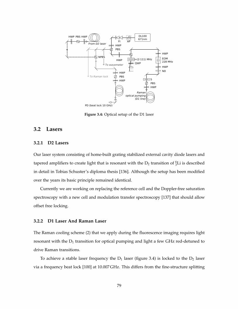
FI AP
PBS
+(2·111)0MHz EOM2280MHz
ND
QWP
S
HWP
PBS
Raman
optical pumping
(D1 line)
HWPHWP
NPBS
To wavemeter
PD0(beat0lock0100GHz)
To Raman lock
HWPPBSHWP
From D2 laser
DL100671nm
HWP
HWPHWP
HWPHWP
HWP
PBS
HWP
Figure 3.4: Optical setup of the D1 laser
3.2 Lasers
3.2.1 D2 Lasers
Our laser system consisting of home-built grating stabilized external cavity diode lasers and
tapered amplifiers to create light that is resonant with the D2 transition of 63Li is described
in detail in Tobias Schuster’s diploma thesis [136]. Although the setup has been modified
over the years its basic principle remained identical.
Currently we are working on replacing the reference cell and the Doppler-free saturation
spectroscopy with a new cell and modulation transfer spectroscopy [137] that should allow
offset free locking.
3.2.2 D1 Laser And Raman Laser
The Raman cooling scheme (2) that we apply during the fluorescence imaging requires light
resonant with the D1 transition for optical pumping and light a few GHz red-detuned to
drive Raman transitions.
To achieve a stable laser frequency the D1 laser (figure 3.4) is locked to the D2 laser
via a frequency beat lock [100] at 10.007 GHz. This differs from the fine-structure splitting
79

TA
HWPPBS
FI
CL
HWP PBSVortexGII671nm
HWP PBS
HWP PBS
Raman light
NPBS
PDG(beatGlockG7GGHz)
From
D1 laser
HWP
PBS
HWP
HWP
Figure 3.5: Optical setup of the Raman laser
because both the D1 and D2 lasers get frequency shifted using acousto-optical modulators
before they reach the atoms. The Raman laser is then locked to the D1 laser via another
beat-lock at 7 GHz.
The beat signal in both cases is detected on a fiber coupled Hamamatsu G4176-03
photodetectors that are biased by a MiniCircuits ZX85-12G+ bias tee. The signal is then
amplified twice with MiniCircuits ZX60-24-S+ amplifiers before the frequency gets stepped
down with a RF Bay, Inc. FPS-6-12 pre-scaler, to bring the frequency into the range of our
frequency detection circuit (below 3 GHz).
3.2.3 High Power ODT
In the experiment sequence (see 3.4.3) atoms from the magneto-optical trap get directly
transferred into an optical dipole trap to perform evaporative cooling. At this stage the
atoms are still relatively hot (about 1 mK) and therefore high laser powers are required to
trap them in a conservative potential of a far off-resonant trap.
Although alternative solutions exist (e.g. cavity-enhanced trapping [138]), in our experi-
ment the deep trapping potential is created by brute-force approach: a 300 W water-cooled
1070 nm frequency multimode, spatial single mode IPG Photonics YLR-300-LP-WC fiber
laser focused to a Gaussian waist of 54µm. The coherence length of this laser is measured
to be 270µm [100]. At full power this should yield a trap depth of about 4 mK – sufficiently
deep to capture atoms directly from a compressed magneto-optical trap.
80
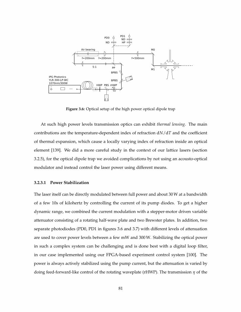
HPND
HWP
PP
PBS rHWP
BPBS
BPBSM1
M0
PD0PD1
ND
f=200mm f=500mmf=200mm
5:1
Airsbearing
IPGsPhotonicsYLR-300-LP-WC1070nm/300W
Figure 3.6: Optical setup of the high power optical dipole trap
At such high power levels transmission optics can exhibit thermal lensing. The main
contributions are the temperature-dependent index of refraction dN/dT and the coefficient
of thermal expansion, which cause a locally varying index of refraction inside an optical
element [139]. We did a more careful study in the context of our lattice lasers (section
3.2.5), for the optical dipole trap we avoided complications by not using an acousto-optical
modulator and instead control the laser power using different means.
3.2.3.1 Power Stabilization
The laser itself can be directly modulated between full power and about 30 W at a bandwidth
of a few 10s of kilohertz by controlling the current of its pump diodes. To get a higher
dynamic range, we combined the current modulation with a stepper-motor driven variable
attenuator consisting of a rotating half-wave plate and two Brewster plates. In addition, two
separate photodiodes (PD0, PD1 in figures 3.6 and 3.7) with different levels of attenuation
are used to cover power levels between a few mW and 300 W. Stabilizing the optical power
in such a complex system can be challenging and is done best with a digital loop filter,
in our case implemented using our FPGA-based experiment control system [100]. The
power is always actively stabilized using the pump current, but the attenuation is varied by
doing feed-forward-like control of the rotating waveplate (rHWP). The transmission η of the
81

rHWP PBSYLRd300dLPdWC
30Wfff300W 3mWfff300W
HPND
PD0PD1
ND
ptcη
Curr
ent
p10
M–1
00
Mc
PSPptc ·p1d99ptccα ·99ptcgα
i1fff4096·1fff65536
Error Measuredment
Errorpredscaler
·GPptc
GIptc∫dt
PI9loopfilter
Figure 3.7: Simplified diagram of the feedback setup to stabilize the output power over a largedynamic range
waveplate polarizer setup as a function of the stepper motor position s and the number of
steps per full period is given by
η(s) = (1− η0) cos2(
πss0
)+ η0 (3.1)
with a maximum extinction η0 ∼ 1/1000. At this high power levels polarizing beam splitter
cubes should be avoided and Brewster polarizers should be used instead.
The small glitches from the finite resolution of the stepper motor and the motor bounce
back are almost completely smoothed out by the active feedback. But when the attenuation
is increased, the loop gain on the other hand effectively decreases. This can become a
problem once the loop gain is too low to filter out the glitches. For example, when the
setpoint is set to 50 W, but the current measurement is 60 W, the error is just 10 W, if there
is no attenuation at all. If, however, the transmission is set to 1/2 and the measured power
after the attenuation again is 60 W, the laser is actually outputting twice that, namely 120 W.
Although the measured error is still only 10 W, the laser pump current is an equivalent of
20 W too high. Hence the proportional and integral gain GP,I should always be inversely
proportional to the attenuator transmission η
GP,I =G(0)
P,I
η. (3.2)
Since the gain needs to be adjusted over three orders of magnitude or 10 bits, the error
82

is first multiplied by an factor of 2p (p = −12 . . . 16) to preserve enough significant bits
without running into truncation errors.
3.2.3.2 Closed Loop Ramp
During the first part of the optical evaporation (3.4.4) the laser power is ramped down to
30 W. This is done by reducing the pump current until the power setpoint is at 50 W and
then the attenuator transmission is adjusted such that for any given setpoint Pset the actual
laser output power Plaser stays around P0 = 50 W:
η(t) =Pset(t)
P0(3.3)
The stepper motor position is then calculated from the setpoint Pset by inverting equation
(3.1) while assuming perfect extinction η0 → 0. From this point on the evaporation is done
by feeding forward on the attenuator, the loop filter only needs to make small adjustments
to the pump current.
When the laser power is ramped down further and reaches about 8 W, a hand-over
between the high and the low power photodiode is performed. The measurement input
Vmeas of the loop filter can blend between the low power photodiode Vlow to the high power
photodiode Vhigh
Vmeas = (1− α(t))Vhigh + α(t)gVlow, (3.4)
where g is the ratio of the laser power to voltage gains of the high and low power photodiodes
and α(t) linearly changes from 0 to 1 in time. This procedure is somewhat related to fuzzy
logic [100]. Once the transmission of the attenuator is limited by the finite extinction η0 at
laser powers of about 100 mW the loop filter compensates and starts to reduce the pump
current to get to the desired setpoint.
3.2.3.3 Noise Performance
Fluctuations in the laser power on a timescale faster than the feedback bandwidth can
lead to heating of the trapped atoms. Compared to our lattice lasers (3.2.5) the IPG fiber
83

0 100 200
−100
−80
−60
Frequency (kHz)Rin(dBc/Hz)
40W 288W
Figure 3.8: Residual amplitude noise of the IPG laser at different output powers
laser exhibits are large amount of residual amplitude noise with multiple peaks reaching
to almost −60 dBc/Hz and a baseline noise between −100 dBc/Hz and −80 dBc/Hz depending
on the output power level (see figure 3.8). This behavior is expected for an industrial laser
designed for material processing. But besides it relatively high noise levels it has been
working very reliably over the years. We avoid potential heating issues due to the amplitude
noise (1.4.4) by only using this laser for the initial evaporation, while the atoms are still
comparably hot and then hand over to different traps with almost negligible heating rates.
3.2.4 Dimple
In our experiment the atoms are trapped a few ¯m below a glass surface (see 3.3.1). Any
beam hitting the atoms from the vacuum side of this surface is inevitably going to be
partially reflected, even with a good anti-reflection coating. This reflection will form a
standing wave pattern below the substrate.
To circumvent this problem, we send in beams from the glass side of the interface
through our microscope objective (see 3.3.5). Since the objective contains multiple lenses,
double reflection could still cause the light to interfere in the forward direction. By using an
incoherent light source with a coherence length less than the typical thickness of a lens (few
millimeters), multiple reflections do not interfere in the focus of the trap and cause short
wavelength potential corrugations/disorder.
84

SLED785nm
HWP
HWP
HWP
PBS
PD
PD
BP
BP
1:2
CL
3:1
FI
TA
HWPPBS
PD
PBS HWPHWP
HWP
HWP
HWP
FM
1:3
CL
FI
TABP
+136 MHz
BP
S
HWP PBS
PD
BP -81 MHz
HWP S
¨Tiny¨ dimple
¨Big¨ dimple
Figure 3.9: Optical setup of the low power optical dipole traps
To provide additional axial confinement in the high-power dipole trap (3.4.6) and during
the accordion compression (3.4.7) we shine ∼700 mW broadband light through our objective.
3.2.4.1 Incoherent Light Source
The incoherent light for the tapered amplifiers is generated by a fiber-coupled Exalos
superluminescent diode with a center wavelength of 786 nm and a bandwidth of 12 nm
outputting 7.6 mW of incoherent light, 5.7 mW in a single polarization. With the temperature
and current controller provided by Exalos the residual amplitude noise spectrum showed
peaks at 157 kHz (−107 dBc/Hz), 316 kHz (−116 dBc/Hz), and 997 kHz (−98 dBc/Hz). Replacing
these with Thorlabs TEC200 and LDC202C resulted in a flat noise spectrum from 50 kHz
to 1 MHz at a level of −128 dBc/Hz.
3.2.4.2 Tapered Amplifier
The power from the incoherent light source is not sufficient to fully saturate an Eagleyard
Photonics 780 nm, 2.2 W output power tapered amplifier. Therefore we use a two-stage
85

SMAuconnector(power)
Taperedamplifier
6mmuholes(30mmucageusystem)
Peltieruelements
Thermistor
Waterucooling
Insulator(MACOR)
Figure 3.10: Picture of the tapered amplifier mount
tapered amplifier design to obtain powers > 2 W out of the second stage amplifier for a seed
power of 30 mW and a current of 3.9 A. When carefully mode matched with a cylindrical
lens, powers > 1.1 W can be achieved after a double-stage optical isolator and a single-mode
fiber. Optimizing for fiber coupling efficiency is different from maximizing the bare output
power of the tapered amplifier. It seems that the tapered amplifier is not purely single mode
and can support multiple spatial modes. Lasing at multiple modes gives an overal higher
output powers for the same electric current and seed power, but the fiber coupling efficiency
is reduced.
At full power the tapered amplifier produces about 8 W of heat that is extracted using
two water-cooled TE Technology, Inc. TE-71-1.4-1.5 Peltier thermoelectric coolers in series,
stabilizing the temperature to 19.5C at a steady-state current of 0.5 A.
Since the output facet of the tapered amplifiers is very elongated the divergence along the
horizontal and vertical axis is vastly different. First the weakly diverging axis is collimated
with a short focal length aspheric lens. Then the waist size along the other, still diverging
axis is mapped out with a beam profiler along the optical axis and fitted to the waist of a
propagating Gaussian beam w(z− z0) with the initial waist w0 and the waist location z0 as
free parameters. This procedure assumes a perfect Gaussian beam. Allowing for a finite
M2 > 1 tends to give worse fit results. Once these parameters are known, one can read
off the distance from the waist location z0 to the point where the waists along both axes
86
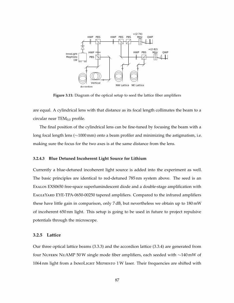
HWP PBS HWP PBS+(2·74)
MHz QWPPBS
+(2·82)MHz QWPPBS
PBS
HWPHWP
NWnLattice NEnLatticeVertical
Accordion
InnoLightMephisto
1W
Figure 3.11: Diagram of the optical setup to seed the lattice fiber amplifiers
are equal. A cylindrical lens with that distance as its focal length collimates the beam to a
circular near TEM0,0 profile.
The final position of the cylindrical lens can be fine-tuned by focusing the beam with a
long focal length lens (∼1000 mm) onto a beam profiler and minimizing the astigmatism, i.e.
making sure the focus for the two axes is at the same distance from the lens.
3.2.4.3 Blue Detuned Incoherent Light Source for Lithium
Currently a blue-detuned incoherent light source is added into the experiment as well.
The basic principles are identical to red-detuned 785 nm system above. The seed is an
Exalos EXS0650 free-space superlumindescent diode and a double-stage amplification with
EagleYard EYE-TPA-0650-00250 tapered amplifiers. Compared to the infrared amplifiers
these have little gain in comparison, only 7 dB, but nevertheless we obtain up to 180 mW
of incoherent 650 nm light. This setup is going to be used in future to project repulsive
potentials through the microscope.
3.2.5 Lattice
Our three optical lattice beams (3.3.3) and the accordion lattice (3.3.4) are generated from
four Nufern NuAMP 50 W single mode fiber amplifiers, each seeded with ∼140 mW of
1064 nm light from a InnoLight Mephisto 1 W laser. Their frequencies are shifted with
87

Nufern NuAMP1064nm/50W
HWP FRFRBPBS BPBSHWP
vWPHWPBPBS HWP
To glass cell
±80 MHz
SPD1
PD0
Figure 3.12: Diagram of the optical fiber amplifier power stabilization setup
acousto-optical modulators (figure 3.11).
For future experiments we wanted to potentially allow interference between the two
radial lattice beams. Therefore their frequency is made tunable by using double-pass
acousto-optical modulator setups. In addition to tuning their frequencies from 74 MHz and
82 MHz to 78 MHz, the polarizations of the lattice beams (3.3.3) will need to be rotated to
be p-polarized with respect to the substrate.
3.2.5.1 Power Stabilization
In the experiment we need to be able to stabilize the power of the lattice beams at low power
levels of O(10 mW) for lattice depths in the Hubbard regime, as well as at high power
levels O(10 W) during the imaging. Each of the four beamlines has a galvo (Thorlabs GVS
or Cambridge Technologies) with a z-cut quartz plate that acts as a variable waveplate
depending the galvo angle. In combination with a polarizer this is used as a high-dynamic
range attenuator. The beam displacement from the tilting plate is negligible since only small
angle changes are necessary to change the retardation by λ/2.
In the low power regime (> 150 mW) the variable attenuation stage is held at a constant,
low transmission. The actual power stabilization is done using a Crystal Technology,
Inc. AOMO 3080-197 80 MHz acousto-optical modulator, whereas at high power levels the
88

modulator is operated at maximum diffraction efficiency and the power is controlled via
slow digital PI feedback onto the galvo directly.
To have the lowest possible amount of noise added from the power stabilization, at low
power levels the rf power going to the acousto-optical modulator is controlled with a mixer
driven by a purely analog PI loopfilter designed in our group. To counteract the quadratic
dependence of the mixed power on the control voltage, the loopfilter board has a built-in
diode circuit that approximates a square-root transfer function.
The ∼80 MHz radio-frequencies are created by phase-locked-loop boards based on an
Analog Devices ADF4002 locked to our lab rubidium frequency standard. This source
has better noise properties than our DDS synthesizers while still being able to tune the
frequencies to a particular value.
As for the high-power optical dipole trap (3.2.3), the laser power is measured with two
photodiodes to cover a large range of power levels without sacrificing noise performance.
Small fractions of the beam are split off with a single Thorlabs BSF10 beam sampler. The
uncoated side of the fused-silica wedge is providing the signal for the low power photo
diode, the weaker reflection off the side with anti-reflection coating is used for the high
power stabilization.
3.2.5.2 Thermal Lensing
The fiber amplifiers were shipped with an f = 25 mm BK7 collimation lens. This material is
known [139] to show a large amount of thermal lensing. We have observed thermal lensing
with LightPath Technologies GRADIUM lenses, lenses with an axial gradient index that
compensates for spherical aberrations.
In addition to the lensing issues with the original fiber collimator, the collimation lens is
also mounted on-axis with the Losch LD-80 receiver, but the fiber itself is angle cleaved at a
4 angle, causing aberrations. In this case the beam from the fiber hits the collimation lens
off-centered and under an angle.
We avoided both problems by using custom machined monolithic copper mounts that
89

take the polishing angle into account and by choosing OptoSigma 027-0510 f = 20 mm
fused-silica air-spaced triplet fiber laser focusing lenses for collimation. The large copper
block also provides a good heat sink.
Other sources of thermal lensing are the optical isolators (two 30 dB stages, Thorlabs
IO-5-1064-VHP) that are required to avoid back-coupling the retro-reflected lattice beams
into the amplifiers. This would (and did) immediately destroy the fiber amplifier. Also the
thermo-optic dependence of the Faraday rotation causes the isolation to change with optical
power [140].
We replaced the cube polarizers in the isolators by Precision Photonics Brewster plate
polarizers and only using the original faraday rotator. Since we are always running the fiber
amplifiers at a constant output power and attenuate the beams further downstream, we
can tolerate potential thermal lensing from the terbium gallium garnet faraday rotator. In
addition, the isolators are mounted on water-cooled bases removing any excess heat.
Our acousto-optical modulators are also water-cooled to stabilize the temperature of
the crystals and to avoid heating the optical table. No degradation of beam quality in first
diffraction order has been observed. In the experiment the power at the acousto-optical
modulators is below 200 mW most of the time, because the beam is already attenuated with
the variable attenuators.
3.2.5.3 Noise Performance
The optical lattice lasers are most critical for the operation of the experiment. To achieve
high fidelity quantum states heating caused by technical noise needs to be minimized. The
biggest contribution herefore comes from the amplitude noise of the laser (see 1.4.4).
The seed laser alone has an impressively low noise floor of about −155 dBc/Hz, but the
amplifiers (although in the saturated regime) add more noise on top of that. There are both
technical and physical noise sources in the amplifiers.
NuFern in Conneticut generously let us take measurements on one of their test systems,
before we ordered our own amplifiers. We minimized the stimulated Brillouin scatter-
90

0 500 1,000−150
−140
−130
−120
Frequency (kHz)Rin(dBc/Hz)
open-loopclosed-loop
Figure 3.13: Measured residual amplitude noise of a lattice laser beam in open-loop and with activepower stabilization
ing [141] in the delivery fiber by shortening them to 50 cm. Since stimulated Brillouin
scattering depends exponentially on the laser power, the amplifiers are not running at the
full 50 W output power. There is also a broad peak in the spectrum at around 0.7 MHz
caused by the relaxation oscillations in the laser medium. It can be completely suppressed
by the built-in noise eater in the Mephisto seed laser.
Besides those two sources producing broadband noise, there were many discrete peaks
caused by various switching power supplies. We suppressed most of those peaks by adding
MPE DS26387 line filters to the pump diode power supply, replacing the MeanWell SP-75-
24 power supplies driving the first stage and some of the electronics with a linear supply,
and replacing the National Instruments USB-6008 OEM USB interface with a home-built
galvanically isolated interface board. All the power supplies are now located outside the
fiber laser enclosure.
Relocating the power supplies also solved a vibration issue: the fan of the power
supplies caused the fiber tip to vibrate. These pointing fluctuations were clearly visible on a
four-quadrant photo diode.
With all those modifications we significantly improved the residual amplitude of our
lattice laser system and only add less than 10 dB of noise in the whole amplification process
compared to the bare Mephisto noise floor. The achieved noise spectrum is shown in figure
3.13.
91

13mm
y
z
x
1.8mm
11.5mm
f=10mmNA=0.60
NAeff=0.88
Figure 3.14: Diagram of the microscope setupon the glass cell
θ
θ'
n=1.46
n'=1
Figure 3.15: Enhancement of the numericalaperture by a hemispheric lens
3.3 Optics
3.3.1 Vertical Imaging: The Microscope
The heart of the imaging system consists of a commercial long working distance objective
optem High-Resolution 20X 28-20-46-00 (post-selected to have less than λ/10 transmitted
wavefront error) with a numerical aperture of 0.60, a focal length of f = 10 mm, and a
working distance of 13 mm (see figure 3.15). Interestingly the objective is designed such that
the principal plane [86] on the object side lies outside the physical objective, thus allowing a
long working distance while still having a short focal length. The back principal plane lies
11.2 mm inside the objective.
3.3.1.1 Optical Resolution
To further enhance the optical resolution the microscope is combined with a hemispheric
lens with a radius of curvature of R = 11.5 mm. That hemisphere is formed by three glass
pieces. On the objective side there is a ground down hemisphere with the same radius of
curvature and thickness of 4.65 mm made by Rocky Mountain Instrument Co. from fused
silica. It is resting on the 5 mm thick glass cell (see 3.1.2) and glued in place with three drops
of low outgassing Torr Seal epoxy along the perimeter. On the vacuum side we optically
contacted (see 3.3.1.2) a 1.8 mm thick superpolished substrate from Gooch & Housego
92

with a combined mirror (for 1064 nm) and anti-reflection coating (671 nm and 780 nm) by
Advanced Thin Films on the vacuum side that also serves as a mirror for the optical lattice
setup (see 3.3.3) and was designed in our group. To guarantee flatness the back of the
substrate is coated with silica. Without this compensation coating the stress induced by the
anti-reflection/mirror coating on the other side would warp the thin substrate.
The center of the hemisphere is concentric with focus of the microscope. Rays from
an on-axis collimated beam that then gets focused by the objective enter the hemisphere
normal to the surface. Thus there is no refraction on this interface. But when the rays exit
on the bottom, going from an index of refraction of n = 1.46 to vacuum with n′ = 1, the
rays get refracted according to Snell’s law [86]
n sin θ = n′ sin θ′. (3.5)
For the marginal rays this directly gives the enhancement of numerical aperture NA = n sin `
of
NAeff = nNA (3.6)
Alternatively in the limit where the object (i.e. the atoms) are very close to the surface
(less than a Rayleigh range) the hemisphere can also be understood as a solid immersion
lens [142].
The maximum resolution that could be achieved theoretically with this setup with an
effective numerical aperture of NAeff = 0.88 would be (the so called Rayleigh criterion [86])
∆r =1.22
NAeff
λ
2= 467 nm, (3.7)
but as described later, our system suffers from spherical aberration, because the object
plane is not exactly at the superpolished surface (see 3.3.1.4). Correcting these aberrations
by going away from infinite conjugation is going to slightly reduce the optical resolution.
Simulations in Zemax indicate that in the corrected system’s resolution should be about
475 nm, still smaller than the lattice spacing of 566 nm.
93

3.3.1.2 Optical Contacting
Mounting optics inside an ultra-high vacuum chamber is a challenge, because only low
outgassing materials can be used. This excludes any (even low outgassing) glues. An
additional complication in our experiment is the high laser power. Even a small fraction of
the overall power absorbed on a metal piece in vacuum would heat it up quickly, because it
only thermalizes through radiation unless it is heatsunk somehow to the air side. There
obviously is no convection cooling in vacuum.
We decided to optically contact the superpolished substrate to the glass cell, a process
where two sufficiently flat and clean glass surfaces bond together by van-der-Waals forces
and hydrogen bonds — completely without any adhesive.
Superpolished substrate cleaning The superpolished substrates arrived already reason-
ably clean from the coating run. It is important that the edges are beveled and polished
so that there are no glass crumbs being dragged across the superpolished surface in the
cleaning process. Fused silica is hard enough to scratch fused silica (so are most metals that
have a protective oxide layer, like aluminum, titanium, non-stainless steel)! Light scattering
from imperfections in the surface can later create disorder in our optical potentials. Since
the electric fields directly enter the interference term, not the intensities, a small amount
of scattered light can create a surprisingly large corrugation. For example, 100 ppm scatter
creates 1% disorder.
To remove residual dust particles the substrate was mounted on a MTI VTC-100 spin
coater under a HEPA filter and spun at 2000 rpm. The spinning glass piece was flushed
with high purity isopropanol C3H7OH and wiped several times radially from the center
outwards with Coventry 52121 pillow tip swaps while still flushing it with isopropanol.
The solvent was then flushed away with plenty of HPLC grade water H2O and the substrates
blown dry with ultra-high purity nitrogen gas N2.
Attempts to etch/activate the superpolished surface with an aqueous solution of potas-
sium hydroxide KOH failed, leaving a permanent milky finish on the surface, probably
94

because it increased the surface roughness, and attacking the anti-reflection coating.
Glass cell polishing and cleaning Our weapon of choice for cleaning the glass cell is
RCA1 solution [143], a mixture of one part by volume 33% ammonia NH4OH, two parts
30% hydrogen peroxide H2O2 (not stabilized), and seven parts HPLC grade water H2O.
It is used in the semiconductor industry and it can remove organic as well as particulate
contamination. In addition it can alter the surface termination and create hydroxyl groups
that aid the optical contacting to other surfaces. This effect is known as chemically activated
bonding.
A first cleaning step was performed, removing all major contamination by the following
procedure:
1. Sonicate2 glass cell filled with RCA1 in a large beaker of pre-heated RCA1 at 80C for
1 min.
2. Flush thoroughly with HPLC grade water H2O.
3. Wipe outside of the glass cell with lint-free lens paper Berkshire Lensx 90, semi-
conductor grade methanol CH3OH, and a large hemostat and a good amount of
pressure.
It is important that the solvent bottles have not been opened before. Pure solvents attract
water from the humidity of the air. After a few hours of exposure (even with the lid on) the
water causes residue after the cleaning process.
To remove the remaining glass particles on the inside surfaces (see section 3.1.2) we
tried several ways of polishing. The first attempt to use a modified electric toothbrush with
a polishing pad glued to it turned out to be too tedious. A specially designed polishing
jig made a more controlled process possible, but removed too much material (many λ in
thickness). At the end it turned out to be sufficient to use 250 nm polishing paste (with
rounded particles) directly on a polyester swap and only slightly scrub the inside only to
2Many people discuraged use of a ultrasound bath, because it could potentially undo the bonds. We havesonicated our glass cells many times without a single incident. Most likely this was possible, because our cellshad been heated/annealed multiple times at various production steps as indicated by the degradation in surfaceflatness. I would not recommend to sonicate a “proper” glass cell.
95
remove particles stuck to the surface without repolishing the surface itself.
After the polishing the inside was now contaminated with polishing paste. This time
more thorough cleaning steps were required:
1. Flush the inside with tap water under high pressure e.g. from a faucet, forced through
a small nozzle.
2. Rinse with deionized water.
3. Blow dry with ultra-high purity dry nitrogen N2 through with a 1µm particle filter.
4. Repeat until there is no more residue from the (oil of the) polishing paste visible.
5. Soak in dichloromethane CH2Cl2 for 10 min.
6. Rinse with deionized water.
7. Fill with RCA1 and soak in RCA1 at 80C for 25 min.
8. Sonicate in the RCA1 solution for 30 s.
9. Flush thoroughly with HPLC grade water.
Optical Contacting Since the glass cell was slightly concave after the flange had been
fused on, mechanical force had to be applied inwards to bend the glass cell face until the
inner face was convex (approximately one fringe over 1 cm). The pressure was applied by
carefully tightening screws that pressed down a “X” shaped holder that, in turn, pressed on
a thin Teflon ring sandwiched between the cell and a 1 in glass blank. The whole bending
process was monitored in real-time in an white light interferometer and a low magnification
microscope.
For the optical contacting the superpolished substrate was wetted with 3µl of HPLC
grade water. Adding a small amount of water can help, because it is possible to bond
surfaces over a larger distance with the help of several hydrogen bonds in the gap [143].
The substrate itself was resting on a small lip on top of an inverted brass cone that was
sitting in a hole of a long 1/4 in thick stainless steel bar. This way the substrate could still tip
and tilt to conform to the surface in case the bar was not perfectly parallel to the glass cell.
The plan was to lower the glass cell onto the substrate to perform the contacting. But when
we slightly tapped the stainless steel bar with the substrate already parked below the correct
96
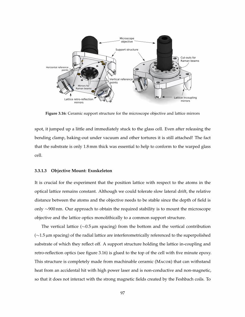
Lattice retro-reflectionmirrors
Microscopeobjective
Support structure
Vertical referencepoints
Horizontal referencepoints
Mirrors forRaman beams
Lattice incouplingmirrors
Cut-outs forRaman beams
Figure 3.16: Ceramic support structure for the microscope objective and lattice mirrors
spot, it jumped up a little and immediately stuck to the glass cell. Even after releasing the
bending clamp, baking-out under vacuum and other tortures it is still attached! The fact
that the substrate is only 1.8 mm thick was essential to help to conform to the warped glass
cell.
3.3.1.3 Objective Mount: Exoskeleton
It is crucial for the experiment that the position lattice with respect to the atoms in the
optical lattice remains constant. Although we could tolerate slow lateral drift, the relative
distance between the atoms and the objective needs to be stable since the depth of field is
only ∼900 nm. Our approach to obtain the required stability is to mount the microscope
objective and the lattice optics monolithically to a common support structure.
The vertical lattice (∼0.5µm spacing) from the bottom and the vertical contribution
(∼1.5µm spacing) of the radial lattice are interferometrically referenced to the superpolished
substrate of which they reflect off. A support structure holding the lattice in-coupling and
retro-reflection optics (see figure 3.16) is glued to the top of the cell with five minute epoxy.
This structure is completely made from machinable ceramic (Macor) that can withstand
heat from an accidental hit with high power laser and is non-conductive and non-magnetic,
so that it does not interact with the strong magnetic fields created by the Feshbach coils. To
97

NPBS
M1
M0L0
HWP
PBS
d
L2f=1000mm
Fizeauplate
x,y,zθp,θyCMOS
L4(opt.)
L1f=200mm L3
Figure 3.17: Objective alignment with delay line and Fizeau interferometer
provide a stable point of contact with glass three short brass pieces with round polished tips
are rigidly screwed into the ceramic piece. To constrain the support in the horizontal plane
we have three little brass cylinders that contact the outside of the glass cell. Brass has low
electrical conductivity, is non-ferromagnetic (unlike stainless steel), and most importantly
does not scratch glass (unlike aluminum, titanium, or most other metals with an oxide
layer). The kinetic mirror mounts for the retro-reflectors are made from Macor as well.
Only the Newport adjuster screws are from stainless steel.
After the objective had been correctly aligned (see next chapter 3.3.1.4) it was glued
into a ring that is screwed to the support structure. Fine focusing is done using the camera
position. If the objective ever has to be realigned, it is possible to undo the screws and swap
out the objective including mounting ring.
3.3.1.4 Objective Alignment
To get the best optical performance the microscope objective needs to be aligned interfer-
ometrically to the hemisphere (concentric) and the superpolished substrate (normal). A
conventional interferometer typically uses coherent laser light to interfere a reference beam
with a reflected beam. In the case of a microscope objective with many internal lens surfaces
there would be too many reflection to identify each surface individually. A solution to this
problem is to use an incoherent light source and a white light interferometer, where the path
lengths in both arms have to match within the coherence length of the light.
98

LP+BP
f=500mm
f=10mm
f=100mmf=100mm
f=150mm
Intermediate
image plane
(low res.)
Figure 3.18: Optical setup for the high resolution vertical imaging with optional de-magnificationfor debugging purposes
Although in our setup we used the incoherent light from a superluminescent diode
(see 3.2.4), it is conceptually easier to think about a pulsed laser. For simplicity of the
setup near the objective we used a Fizeau interferometer [144], but there is no possibility
to independently vary the path lengths of the interferometer arms. To circumvent this
limitation a fiber-coupled optical delay line with a Michelson interferometer [86] (see figure
3.17) is used to generate incoherent light that has a tunable interference revival. Using a cat’s
eye reflector consisting of a lens and a flat mirror, the delayed arm remains fiber coupled
while varying the distance d to “scan” through various glass surfaces inside the objective
and the hemisphere. Only the reflected beams from the Fizeau plate and the “selected”
surfaces interfere on the CMOS camera. For coarse alignment an additional lens L2 can be
introduced to image the Fourier plane, where the reflected beams are just dots that need to
be overlapped.
During the whole alignment process the objective is mounted on mirror mount with two
rotational degrees of freedom and a three-axis translation stage, before it was permanently
glued to the exoskeleton with Torr Seal epoxy. In the lateral direction the objective was
focused with a 1 m lens (L1) attached to the back of the objective and then moved towards
the hemisphere with a micrometer by 75µm. This theoretically compensates for spherical
aberation for an object plane 16µm below the substrate. This lens was removed after the
alignment and is not part of the imaging system.
99

3.3.1.5 High Resolution Imaging
The imaging system is completed with a Thorlabs AC508-500-B 500 mm achromatic lens
that images the atomic cloud onto our CCD camera. To align this lens we first setup a
laser beam along the optical axis down into the microscope (without the lens in place) and
made sure that all reflections from the objective lens/hemisphere are being reflected back
into itself. This ensures that both the angle and position of this beam are aligned with the
optical axis of the microscope. Finally the 500 mm lens is placed into the beam such that
the reflection of the lens surface is going back the right way and that the reflections from
the hemisphere/substrate are still aligned with the reference beam as well. Since we are
not using the microscope in an infinite conjugate ratio setup our magnification is M = 130
instead of fAC/ fObjective = 50. A sketch of the whole imaging setup is shown in figure 3.18.
In the coming weeks a custom correction plate will be mounted at the back of the
objective to correct for some higher order aberations.
3.3.1.6 Low Resolution Imaging
The field of view of the high resolution imaging is about 200µm× 200µm. While this is more
than plenty for imaging atoms inside an optical lattice, for time of flight imaging (to measure
temperatures) or alignment we need the option to have a lower magnification/larger field
of view. This is done by creating an intermediate image with lower magnification and then
re-imaging this image with a 4 f setup. This allows us to keep the camera in the same
place as for the high-resolution imaging (3.3.1.5) and just drop in three lenses to reduce
the magnification to ×10 (see gray elements in figure 3.18). The intermediate image plane
allowed us to use a mechanical chopper in the early stages of the Raman imaging (2.9).
3.3.2 Horizontal Imaging
For alignment and debugging purposes we also need to be able to do absorption imaging [85]
a cloud of atoms near (∼100 um and closer) the superpolished substrate (see section 3.3.1)
from the side. It is difficult to image a cloud from the side due to knife-edge diffraction at
100

θ
Shadowimage
Figure 3.19: Absorption imaging of a cloudof atoms near the substrate
substrate
0.0
0.2
0.4
0.6
0.8
OD
Figure 3.20: Atoms in a crossed optical dipoletrap near the substrate with its mirror image
the side of the substrate. This is a well-known problem in the atom chip community [145]
and can be somewhat improved by imaging in reflection under grazing incidence.
This imaging technique introduces another artifact, a double image. It can be understood
as a second image that gets formed by the mirror image of the imaging beam getting
attenuated by the mirror image of the atom cloud (see figure 3.19). Besides allowing to
recover some signal that would be lost otherwise, the distance from the substrate can be
extracted from the images (for rotationally symmetric clouds and/or small angles θ). It is
located right in between the two images (see figure 3.20).
In our setup the imaging laser beam spans an angle of θ = 4.2 with the surface of the
superpolished surface. Only a small fraction of the light is reflected due to the anti-reflection
coating. That in turn means for a reasonably low saturation parameter, very little light gets
actually reflected into the camera path. The atoms then are imaged with an Infinity K2
DistaMax lens with a CF-3 objective (85 mm–98 mm working distance, magnification of
∼3.5, and a theoretical resolution of 1.7 um) onto a PointGrey Flea3 FL3-GE-03S2M-C
(7.4µm pixel size, 648× 488 pixels). Since the substrate blocks almost half of the numerical
aperture of the lens, expected resolution is reduced. In addition even under such shallow
angles a cloud of 50µm horizontal depth, the geometric vertical spread is already about
4µm. A calibration using atoms in the accordion lattice (3.3.4) at a suggests that the effective
magnification in our setup is 2.3(2) µm/px.
101

Nor
thea
stNorthw
est
Northeast Northwest
HWP HWP
Front view Top view
HWP Verticaly
z
x
x
yz
Figure 3.21: Mode matching and focusing optics of the optical lattice
3.3.3 Lattice
The condensed matter problems we are trying to address with our experiment fundamentally
requires the presence of an optical lattice. While in most traditional optical lattice experiment
this is done by overlapping three orthogonal optical lattices [101], our high-numerical
aperture microscope takes away a large amount of the optical access. Therefore an alternative
way introduce the optical lattice has been chosen with its own challenges and benefits that
are described in the following.
3.3.3.1 Lattice Geometry
The optical lattice is created from three Nufern NuAMP 50 W 1064 nm ytterbium-doped
fiber amplifiers seeded by an Innolight Mephisto 1 W Nd:YAG laser (see section 3.2.5).
Since all three lasers are frequency shifted in the current configuration there is no mu-
tual interference (although they could be tuned to create double-well lattices for future
experiments).
Geometrically it is impossible to send in the lattice beams parallel to the superpolished
substrate and still have the atoms be trapped close to it. Our solution to this problem
is to reflect the radial (x + y and x − y direction) lattice beams off the substrate under a
θ ∼ 20 angle and then retro-reflect the beam back into itself (see figure 3.21). This creates
an interfering φ = π/2 lattice pattern (see equations (1.97) and (1.119)) in a horizontal
plane. The distance of the retro-reflector to the atoms was chosen such that the radius of
curvature of the mirror (R = 50 mm) is identical to the wavefront curvature of the Gaussian
102

−5 0 5
−6−4−20
z/λ
(a)
−5 0 5
x/λ
(b)
−5 0 5
(c)
Figure 3.22: Intensity pattern of a completely incoherent beam (a), a coherent beam (b), and aretro-reflected coherent beam (c) reflected off the superpolished substrate with a Gaussian beamwaist ∼O(λ) to exaggerate the differences
beam (1.65). The diffraction causes the radius of curvature to be greater than expected from
geometrical optics. Therefore the mirror needs to be closer than its radius. Fine-tuning of
the position can be achieved by turning all three adjusters of the retro-reflector kinematic
mount by the same amount.
Since there are effectively four beams interfering, namely the incoming beam, the retro
reflected beam, and their mirror images from the reflection on the substrate, the lattice
depth is enhanced by a factor of four (see equation (1.99)) over the case where they would
be just counterpropagating beams. This is especially useful for our imaging (see 2.9), where
we require tight confinement and a deep optical lattice. One downside of this geometry is
that the radial/horizontal (x− y) and axial/vertical (z) confinement is not decoupled.
A second beam in the same geometry, but rotated by 90 around the z axis, provides the
optical lattice in the perpendicular direction in the x− y plane. Looking from the top the
resulting two dimensional lattice in that plane is a conventional non-interfering φ = 0 lattice
with a spacing of 566 nm in both directions. For the lattices to line up in the z direction, the
angles have to be matched better than ±0.3 for the maxima to line up within ±10% of the
lattice spacing of 1.55µm in that direction (see 3.3.3.2).
To increase the vertical (z direction) confinement the third lattice beam is directly reflected
off the substrate at near-normal incidence (∼5 degrees from normal to match the potential
maxima with the large spacing vertical lattice created by the radial lattice beams) giving rise
to a vertical lattice spacing of 534 nm.
103

3.3.3.2 Lattice Alignment
The superpolished substrate in our experiment serves as a reference surface. This signif-
icantly simplifies the alignment. Once one of the lattice beams (including the accordion
lattice 3.3.4) is aligned to the correct spot in the horizontal (x, y) plane, its position on the
substrate can be seen from below by looking at the Rayleigh scatter with a conventional
camera (PointGrey Chameleon) with the infrared filter removed both on the camera itself
and the lens (Edmund Optics 50 mm/ f 2). This allows us to coarsely align all the other
beams to the same spot, including their retro-reflected beams, although the fine alignment
still needs to be done using atoms.
In addition to the pointing the angles with respect to the superpolished substrate of the
radial lattice beams have to be matched as explained above. At the time of this work the
angles have only been matched by centering the beams on the retro-reflectors. Considering
that it is possible to center it better than 1 mm and the retro-reflector is roughly 5 cm away
from the center of the substrate, this procedure should yield in an uncertainty of ∼1. Once
the experiment is setup to only produce a single pancake, this alignment and the overlap
with the 0.5µm vertical lattice is going to become crucial and other means of aligning the
angles have to be found. Possible techniques could be:
• Measure the differential ac Stark shift by imaging atoms in-trap. The shift should be
maximized when all lattices are overlapped.
• Measure the vertical trap frequency. The frequency should be maximized when all
lattices are overlapped. This method is less sensitive, because of the square-root
dependence of the trap frequency.
• Make a molecular Li2 Bose-Einstein condensate and perform Kapitza-Dirac scatter-
ing [146].
• Drive odd vibrational transitions in the vertical lattice created by the first lattice axis
by modulating the depth of the second lattice axis.
104

-2°
-20°
Figure 3.23: The surface of a galvo mirror is imaged onto the superpolished to create a variablespacing vertical optical lattice.
3.3.4 Accordion
To load the optical lattice near the superpolished substrate we first load the atoms into a
vertical one-dimensional standing wave with tunable lattice spacing.
Initially the atoms are loaded into the fifth maximum of a ∼15µm lattice that is then
continuously compressed to 1.5µm spacing while being transported upwards. The detailed
loading and compression procedure is described in more detail in 3.4.7.
The lattice spacing is varied by changing the angle of incidence of the laser beam on the
reflective coating of the superpolished substrate. This is achieved by imaging the surface of
a galvo mirror (Thorlabs GVS301) on the substrate via an 4 f imaging setup consisting of
two OptoSigma 027-0540 f = 50 mm triplet lenses (see figure 3.24). A second Thorlabs
galvo with a t = 3 mm thick anti-reflection coated glass window is used to dynamically
correct the pointing by displacing the beam. The amount of displacement d as a function of
HWP
HWP
PP
Tilt Galvo
Offset Galvo L1L2 L3
f=50mm
Bre
adboard
From fiberamplifier
P
L4f=400mm
Pointingreference
Figure 3.24: Optical setup of the accordion lattice
105

MACOR spacer
Triplet lenses
Galvo mirror
Galvo plate
XY tra
nsla
tion
stage
Figure 3.25: Mechanical setup of the accordion lattice
the angle of incidence θ is given by
d(θ) = t sin(
1− cos θ
n′ cos θ′
), (3.8)
where the interior angle is given by Snell’s law (3.5) n′ sin θ′ = sin θ and n denotes the index
of refraction (n ∼ 1.46 for fused silica).
The 4 f imaging telescope has to have a fairly large numerical aperture to cover the 20
angle range. This in turn requires the optics to be close to the glass cell and the Feshbach
coils. To minimize eddy currents while still being non-ferromagnetic and structurally very
rigid, the vertical bread board shown in figure 3.25 was machined from titanium. The lenses
themselves are spaced with a ceramic tube with threaded brass rings glued on. The brass
rings are slit to minimize eddy currents, although this is a very minor effect compared to
the aluminum housing of the lenses. Fine positioning of the two galvos is achieved with a
x− y translation stage. The positions of the in-coupling mirrors were calculated a-priori, so
106

that they could be mounted directly onto the breadboard.
3.3.4.1 Astigmatism Compensation
The propagation of a laser beam through a tilted glass plates produces aberrations in the
beam. Most dominantly these are astigmatism (different foci for two orthogonal axes) and
coma [144, 86].
It is not straight forward to decide whether that plate should be parallel to the glass
cell or have the opposite tilt. Those two cases correct different aberrations. For our beam
parameters simulations with Zeemax that the minimum focus shift (as a function of the
galvo tilt angle) was achieved by introducing an anti-reflection coated glass plate with the
same thickness as the glass cell (t = 5 mm) before the telescope. The compensation plate is
parallel to the side of the glass cell.
3.3.4.2 Accordion Alignment
For the initial coarse alignment we mounted a fiber coupled 1064 nm laser onto the vertical
breadboard. This way we can move the assembly around without having to continuously
realign the laser beam before the breadboard. As for the lattice alignment 3.3.3.2 we can use
the Rayleigh scatter off the superpolished substrate to locate the accordion lattice beam.
Since the Gaussian beam waist is fairly large with 200µm the axial alignment is not
critical and the focus only has to be correct within a Rayleigh length (1.64) zR ≈ 12 cm. It is
more important that the focus is on the axis of rotation of the galvo mirror.
The fine alignment was done by slowly scanning the galvo between the two extreme
angles (2 . . . 20) and adjusting the x− y translation stage until it the spot on the substrate
did not move anymore.
The astigmatism compensation plate (see 3.3.4.1) allows us also to calibrate the galvo tilt
angle within machining and assembly tolerances. Herefore the galvo tilt is adjusted that the
back reflection off the compensation plate goes back into itself. By design this corresponds
to a 10 angle.
107

Imaging
PBS
PBS
PBS
HWP HWP
HWP PP
PD
PD
"Tiny Dimple"
"Big Dimple"
DM
DM
Figure 3.26: Optical setup of the tiny and big dimpletrap
Figure 3.27: Close-up view of the σRaman beam near the hemisphere
3.3.5 Dimples
Under shallow angles the accordion lattice provides very little confinement in one direction.
To counteract it is overlapped with the “big dimple” trap, a perpendicular optical dipole trap
with a ∼30µm Gaussian beam waist that is sent through the microscope objective. To get
such a large feature size in the image plane of the objective it is necessary to focus/collimate
the ingoing beam at the Fourier plane (inside the objective) to ∼80µm. This seems to cause
slight aberrations in the image plane, a ring around the central spot, although we could
never exclude that this was not an artifact of the imaging process.
For an alignment purposes and more efficient cooling [147] we also have a very tight
optical dipole trap with ∼6 um Gaussian beam waist, the “tiny dimple”. A similar trap has
been used recently to produce samples of 6Li with a fixed atom number [148].
The dimple beams get sent into the objective through the transmitted port of a dichroic
mirror (DM) that splits off the fluorescence collection arm directly over the back of the lens.
A second dichroic mirror combines the blue- and red-detuned lasers (see 3.2.4) at 650 nm
and 785 nm.
All those beams can conveniently be aligned to the hemisphere. Coming out of the
objective there are two major reflections: one reflected off the bottom of the superpolished
substrate, and one from the hemisphere. The latter one is less sensitive to changes in
the input alignment, because the hemisphere and the superpolished substrate for a “cat’s
108

PBS
NPBSHWP
HWP
π
σ
HWPQWPGTQWP
-(2·243.2) MHz
-258.2 MHz
HWPQWPGT
PBS
HWP
HWP PBS HWP HWP
(Nor
thea
st)π
Raman(N
orthwest)
σ
Raman
Pumping
(top view)
Figure 3.28: Optical setup of the Raman beams
eye” retro-reflector. Also the two reflection move the opposite direction. When all those
reflections overlap, the beam is centered under the hemisphere.
3.3.6 Raman
To avoid differential phase noise between to the Raman legs, the Raman light originates
from a single fiber and is then split in two on the optical table of the experiment. The π-
component is shifted with a single pass that is also used to pulse the beam, the σ-component
is shifted and shuttered with a double-pass acousto-optical modulator. By choosing the
double-pass frequency one can control the two photon detuning of the Raman beam. The
frequencies are also chosen such that electronic crosstalk between the two acousto-optical
modulators is minimized.
The optical pumping beam is overlapped with the σ-polarized Raman beam and sent
into the chamber through the hemisphere outside the numerical aperture of the objective
sin θ = 0.60 (⇒ θ = 36.9), which limits the available angle range on one side. On the other
side the angle is limited by the total internal reflection angle
θTIR = arcsin1n′
= 42.3. (3.9)
109

M1
M0
f=200mm f=500mmf=200mm
5:1
Air bearing
From IPG laser
Figure 3.29: Optical setup of the high power dipole trap
We mounted eight small angle mirrors directly to the microscope objective, which
allow us to send the beam into the hemisphere under an angle that is compatible with the
constraints. A beam path is depicted in figure 3.28. In this configuration the Raman and
optical pumping beam is along one of the radial lattice axes and ∼15 titled away from the
superpolished substrate.
The π-polarized Raman beam on the other hand is introduced from below through the
back of one of the lattice incoupling mirrors along the orthogonal radial lattice axis and
∼20 from the substrate. The whole setup is visualized in setup in figure 3.28.
3.3.7 High Power Optical Dipole Trap
The laser beam is focused onto a ∼20µm spot with a f = 200 mm lens that is mounted
onto a Aerotech ABL10100 air bearing stage with ∼100 mm of travel. The ability to move
the focus allows us to transport atoms in an red-detuned optical dipole trap [149]. A 4 f
imaging system with a magnification of ×2.5 enhances the effective travel by a factor of
2.52 = 6.25 and enables us to transport over a distance of > 60 cm from the main chamber
into the science chamber. The transport sequence is described in great detail in section 3.4.5.
In addition the second to last kinetic mirror mount M0 is motorized with two Newport
PicoMotors to align the position of the optical dipole trap in the science chamber on a daily
basis. For continuous control over the vertical distance from the super polished substrate,
another adjuster on M1 is controlled with a large-travel piezo.
110

Slowing
beam
Atomic
beam
Figure 3.30: Coil pattern of the Zeeman slower
3.4 Sequence
3.4.1 Atomic Beam Source
The atomic beam emerges from a two-species sodium-lithium oven base on the MIT de-
sign [150]. For the experiments described in this work the sodium section has been turned
off, with only the sodium nozzle left at 400C. The lithium reservoir is heated to 380C,
being well in the liquid phase and giving a vapor pressure on the order of 10−4 torr [151].
To prevent clogging and formation of a sodium-lithium alloy the nozzle itself is heated to
450C.
Downstream the beam is collimated by a 0.4 in bore in a copper coldplate at room
temperature and then shuttered with a thin copper sheet mounted to a UHV Design
MagiDrive magnetic rotary feedthrough operated by a hobby grade servo motor.
After five years of moderate operation the coldplate shows a significant layer of alkali
metal, a few millimeter thick. Most certainly this is caused by the high sodium flux in
the early stages of this experiment, but should not pose a problem in the current mode of
operation with only lithium.
3.4.2 Zeeman Slower
In a Zeeman slower [57] atoms from an atomic beam moving at a velocity v get continuously
slowed down by a counterpropagating resonant laser beam with the wavevector |kL| = 2π/λ.
To compensate for the change in doppler shift −kL · v due to the deceleration, a spatially
varying magnetic field Zeeman shifts the atom transition back into resonance to fulfill the
111

−1 −0.8 −0.6 −0.4 −0.2 0 0.2
−500
0
500
Distance from MOT center x (m)
Vert
.m
ag.
field
B(x
)(G
)
Figure 3.31: Calculated magnetic field profile of the Zeeman slower
resonance condition
− 1h
µ · B(z)− kL · v(z) + δ = 0, (3.10)
where δ = ωL − ω0 denotes the detuning of the laser frequency ωL from the atomic
resonance at zero field ω0. The difference in magnetic moment µ of lithium atoms in the
stretched states∣∣22S1/2(F = 3/2, mF = ±3/2)
⟩and
∣∣22P3/2(F = 5/2, mF = ±5/2)⟩
is equal to
one Bohr magneton |µ| = µB. A more detail description of the theory and design of our
Zeeman slower can be found in [134].
After the sodium section of the oven had been retired, the Zeeman slower parameters
were re-optimized to maximize the capture efficiency for the lithium atoms emerging from
the oven. By running the slower at slightly higher currents yielding a magnetic field ranging
from B0 = −707 G to 505 G (figure 3.11). By increasing the detuning to δ = −800 MHz, the
capture velocity
vcap =µh B0 − δ
kL(3.11)
increases to 1200 m/s.
Integrating up the velocity profile of the atomic beam [152]
dN(v)dv
= 2Nv3
v4p
exp
(− v2
v2p
)(3.12)
112
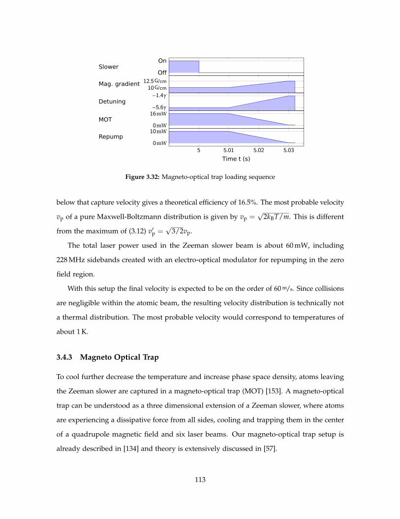
Off
OnSlower
10G/cm12.5G/cmMag. gradient
−1.4γ
−5.6γDetuning
0mW
16mWMOT
5 5.01 5.02 5.030mW
10mW
Time t (s)
Repump
Figure 3.32: Magneto-optical trap loading sequence
below that capture velocity gives a theoretical efficiency of 16.5%. The most probable velocity
vp of a pure Maxwell-Boltzmann distribution is given by vp =√
2kBT/m. This is different
from the maximum of (3.12) v′p =√
3/2vp.
The total laser power used in the Zeeman slower beam is about 60 mW, including
228 MHz sidebands created with an electro-optical modulator for repumping in the zero
field region.
With this setup the final velocity is expected to be on the order of 60 m/s. Since collisions
are negligible within the atomic beam, the resulting velocity distribution is technically not
a thermal distribution. The most probable velocity would correspond to temperatures of
about 1 K.
3.4.3 Magneto Optical Trap
To cool further decrease the temperature and increase phase space density, atoms leaving
the Zeeman slower are captured in a magneto-optical trap (MOT) [153]. A magneto-optical
trap can be understood as a three dimensional extension of a Zeeman slower, where atoms
are experiencing a dissipative force from all sides, cooling and trapping them in the center
of a quadrupole magnetic field and six laser beams. Our magneto-optical trap setup is
already described in [134] and theory is extensively discussed in [57].
113

Initially the magneto-optical trap with ≈ 108 atoms is loaded at a detuning of δ =
−2π · 33 MHz = −5.6γ and magnetic field gradient of 10 G/cm along the weaker axes of the
quadrupole field for 5 s. Each laser beam typically has a laser power of about 16 mW on the∣∣22S1/2(F = 3/2)⟩→∣∣22P3/2
⟩(“MOT”) transition and 10 mW on the
∣∣22S1/2(F = 1/2)⟩→∣∣22P3/2
⟩(“repump”) transition with a Gaussian beam waist w0 ≈ 8 mm. The actual laser
power drifts slightly from day to day, because of slow polarization drifts in the fibers coming
from the Evanescent Optics Inc. polarization maintaining fiber splitter used to combine
the MOT and the repump light.
During the last 20 ms an optical dipole trap (see 3.2.3) overlapped with the magneto-
optical trap is turned on. Its Gaussian beam waist is w0 = 54 um at a maximum laser power
of 255 W and a center wavelength of λ = 1070 nm. This corresponds to a trap depth of
3.3 mK, which is significantly deeper than the temperatures expected in the magneto-optical
trap.
The mode overlap can be improved further by compressing the magneto-optical trap
after the Zeeman slower has been turned off. In our setup this is done by reducing the
detuning to δ = −2π · 8 MHz = −1.4γ linearly over 20 ms, while also reducing the laser
power to 0.6 mW for the MOT light and 0.2 mW for the repump light and increasing the
magnetic field gradient to 12.5 G/cm. This compressed magneto-optical trap (cMOT) is only
a transient effect. In steady state a majority of atoms are lost, when going to very near
detuned light.
By ramping the repump laser faster than the MOT laser, atoms start to get preferentially
pumped into the∣∣22S1/2(F = 1/2)
⟩state, the lowest energy states of the system. There they
are not subject to spin-changing collisions at the high densities in the optical dipole trap.
In our experiment we are not set up to directly measure the temperature in the magneto-
optical trap. But the temperature after the transfer to the optical dipole trap is measured to
be 800µK, which is a few times higher than the Doppler temperature
TD =hγ
2kB= 139µK, (3.13)
114

0 0.2 0.4 0.6 0.8 1
0.4
0.6
0.8
1
1.2
1.4
1.6
·107
Hold time (s)
Atom
number
0 0.2 0.4 0.6 0.8 1300
400
500
600
700
800
900
1,000
Hold time (s)
Temperature
(µK)
750G0G
Figure 3.33: Plain evaporation in an optical dipole trap of 3 mK depth
the theoretical limit for Doppler cooling. A possible explanation for the higher tempera-
tures in the optical dipole trap is the fluctuation dipole force heating caused by the large
differential ac Stark shift on the order of 20 MHz between the∣∣22S1/2
⟩and
∣∣22P3/2⟩
states.
Depending on the exact parameters and the alignment of the magneto-optical trap 1/e
lifetimes of up to 8 min have been measured.
Due to the non-resolved∣∣22P3/2
⟩excited state hyperfine structure conventional sub-
doppler cooling techniques like polarization gradient cooling [57] are not expected to work
for lithium and have not been demonstrated experimentally. Polarization gradient cooling
would require a differential ac Stark shift for the different mF states in∣∣22S1/2
⟩ground
state. Recent demonstrations of gray molasses cooling [154, 155], Sisyphus cooling [156],
and cooling on the ultra-violet∣∣22S
⟩→∣∣32P
⟩transition [157] show ways to circumvent this
limitation and potentially increase the atom number in the optical dipole trap.
3.4.4 Initial Optical Evaporation
After the initial laser cooling we are left with ∼107 atoms in an optical trap with a Gaussian
beam waist is w0 = 54 um created by focusing a 255 W broadband 1070 nm fiber laser
(see 3.2.3, 3.3.7, 3.4.4). Although the temperature of the atoms is already three times less
than the theoretical trap depth of 3.3 mK, the phase-space density (see equation (1.52))
can be increased five-fold by just holding the atoms in the trap at a constant trap depth.
115

106
107
Atom
number
1 10 1001
10
100
Final power (W)
Temp.(µK)
Figure 3.34: Atom number and temperatureduring the optical evaporation in the mainchamber. The solid lines are calculationsbased on Luo et al.[159]
0 10 20 30 40 50 60 70
1
2
3
4
5
Time t (ms)
Positionx(m
m)
Figure 3.35: Center of mass oscillations of theatomic cloud in the optical dipole trap
Collisions inside the trap occasionally produces high energy atoms that then leave the
trap and reduce average the temperature of the remaining atoms. This process is called
plain evaporation [158]. For 6Li atoms the collision rate can be significantly increased by the
increased the interparticle scattering length a near the Feshbach resonance. Figure 3.33
shows the enhanced evaporation at 750 G (a = 3500a0) compared to 0 G (a = −13a0).
In the actual experiment we do not perform plain evaporation to minimize the time that
the science chamber downstream of the dipole trap is exposed to high laser powers, but
instead we immediately start forced evaporation after 5 ms. This has no significant effect on
the atom number.
Forced evaporation is a process where the hottest atoms actively get removed from the
system. In our experiment this is done by continuously lowering the trap depth. In
comparison to evaporative cooling in a magnetic trap using a radio-frequency knife [160],
reducing the laser power for optical evaporation also reduces the trap frequencies and thus
the scattering rate. This is merely a problem, because typically the trap frequencies in optical
traps, especially in a crossed optical dipole trap, are higher than in magnetic traps, leading
to a faster evaporation. In the main chamber, however, we only use a single beam optical
116
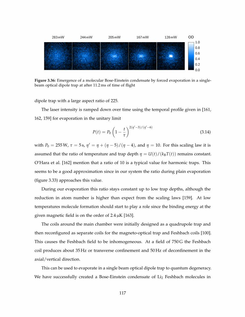
283mW 244mW 205mW 167mW 128mW
0.0
0.2
0.4
0.6
0.8
1.0
OD
Figure 3.36: Emergence of a molecular Bose-Einstein condensate by forced evaporation in a single-beam optical dipole trap at after 11.2 ms of time of flight
dipole trap with a large aspect ratio of 225.
The laser intensity is ramped down over time using the temporal profile given in [161,
162, 159] for evaporation in the unitary limit
P(t) = P0
(1− t
τ
)2(η′−3)/(η′−6)
(3.14)
with P0 = 255 W, τ = 5 s, η′ = η + (η − 5)/(η − 4), and η = 10. For this scaling law it is
assumed that the ratio of temperature and trap depth η = U(t)/(kBT(t)) remains constant.
O’Hara et al. [162] mention that a ratio of 10 is a typical value for harmonic traps. This
seems to be a good approximation since in our system the ratio during plain evaporation
(figure 3.33) approaches this value.
During our evaporation this ratio stays constant up to low trap depths, although the
reduction in atom number is higher than expect from the scaling laws [159]. At low
temperatures molecule formation should start to play a role since the binding energy at the
given magnetic field is on the order of 2.4µK [163].
The coils around the main chamber were initially designed as a quadrupole trap and
then reconfigured as separate coils for the magneto-optical trap and Feshbach coils [100].
This causes the Feshbach field to be inhomogeneous. At a field of 750 G the Feshbach
coil produces about 35 Hz or transverse confinement and 50 Hz of deconfinement in the
axial/vertical direction.
This can be used to evaporate in a single beam optical dipole trap to quantum degeneracy.
We have successfully created a Bose-Einstein condensate of Li2 Feshbach molecules in
117

0Scm
60ScmTransport
255SW
750SG
0SG300SGMag.Sfield
0SW30SW
DipoleStrappower
Mainchamber
Sciencechamber
2.4 4.40TimeSt-t0S(s)
Figure 3.37: Experiment sequence of the all optical transport
this trap geometry. The smoking gun of the condensation is the emergence of the zero-
momentum peak in time-of-flight images (figure 3.36). Before the release from the trap
the intermolecular interaction was reduced by switching of the magnetic field and then
quickly ramped up again during the last milliseconds of the time of flight. This way the
momentum distribution does not get altered by interaction and shows the condensation into
the zero-momentum state. Since this was only done to qualitatively test our evaporation,
there is not exact atom number or temperature measurement, but estimated to have on the
order of 10,000 molecules at a temperature of about 100 nK.
The trap frequency is determined by offsetting the trap minimum slightly during loading
and exciting center of mass oscillations in the longitudinal direction. From the oscillation
frequency ω and the damping coefficient λ of the fit function x(t) = x0 + x′ cos(ωt +
t0) exp(−λt) one can extract the trap frequency for the undamped case
ω0 =√
ω2 + λ2.
For a given laser power it is possible to calculate the Gaussian beam waist from equa-
tion (1.80). The measurement in figure 3.35 indicates that Gaussian beam waist is w0 =
54.1(5)µm. Note that this is ignoring systematic effects from the anharmonicity of the
trap. To determine the trap frequency more accurately one would need to vary the initial
displacement and extrapolate to small displacements.
118

0
0.5
1
Pos.
x/x m
ax
0
0.5
1
Vel.
v/v m
ax
0 0.5 1
−10
1
Time t/tmaxAcc.
a/a m
ax
Figure 3.38: Position, velocity, and acceleration during the optical transport
3.4.5 All-optical Transport
After the first evaporation in the main chamber down to 30 W of laser power the atoms
are at a temperature of about 40µK. The final atom number after a second evaporation is
independent of the transport power over a large range of parameters.
The transport over ∼60 cm into the science chamber is performed by slowly moving the
focus of the optical dipole trap by translating the focusing lens [100]. The position of the
atoms follows a “constant-jerk” profile where the acceleration is ramped piecewise-linearly
in time yielding a piecewise quartic profile in position. For a transport over distance
xmax in the time tmax the maximum required acceleration is amax = 8xmax/t2max and the
maximum velocity is vmax = 2xmax/tmax. The jerk a(t) during the constant acceleration is
|a| = 32xmax/t3max. During the first half of the one-way transport the position is given by
x(t) =
0 t ≤ 0
23
amaxtmax
t3 0 < t ≤ tmax4
amax
(− 4
tmaxt3 + t2 − 3
2 tmaxt + t2max
)tmax
4 < t ≤ tmax2
. (3.15)
The whole profile is visualized in figure 3.38.
At the transport power of 30 W we do not observe any heating or atom loss. Heating rate
in figure 3.39 can be explained solely by the heating caused by the residual intensity noise
on the trapping laser (3.2.3.3). The large spread of temperatures in the plot is attributed to
119

2 3 4 5 6 7 8 9 10
0.6
0.7
0.8
0.9
1
1.1
One-way transport time (s)
Atom
number(a.u.)
no transp.round-trip
2 3 4 5 6 7 8 9 10
42
44
46
48
50
52
One-way transport time (s)
Temperature
(µK)
Figure 3.39: Transport heating for round-trip transport over 60 cm per leg
the poor image quality at zero-field imaging.
During the transport the high-power beam is aligned such that it exits the glass cell at
the center. This leaves the atoms about 10 mm below the super-polished substrate at the end
of the horizontal transport. In the next step the atoms are transported up vertically by tilting
the dipole trap beam via the mirror M2 in figure 3.3.7 with a Piezosystems Jena MICI 200
SG amplified piezo. The vertical translation gain near the substrate is roughly 2 . . . 4 µm/mV.
At this point the cloud is still very elongated along the direction of the laser and cannot
be transported all the way up to its final position near the surface. It is evaporated further a
few 100µm away from the substrate before it is moved closer for the loading of the accordion
lattice (3.4.7).
3.4.6 Final Optical Evaporation
The optical dipole trap is overlapped with a secondary dipole trap (see 3.3.5) formed by a
785 nm incoherent beam with 0.5 W of power and a Gaussian beam waist of 28µm. This
trap should theoretically be 55µK deep, so that all atoms should “fall” into this trap right
after the transport. But compared to the high-power dipole trap alone the volume is smaller
so that it only becomes visible after further evaporation, hence the name “big dimple” trap.
For alignment purposes mirror M1 in figure 3.3.7 is equipped with two NewFocus
Picomotors. Although we cannot move them in real-time, they are a valuable tools to do
120

0.1 0.3 0.54.5
5
5.5
6
6.5
7
Time t (ms)
Width
(a.u.)
Figure 3.40: Oscillations of the cloud sizeafter a quench of the trap depth of the “bigdimple”
0.0
0.5
1.0
1.5
OD
Figure 3.41: Degenerate Fermi gas of N ∼30000 atoms at a temperature T/TF ∼ 0.2after 0.87 ms time-of-flight
the fine alignment to overlap the high-power optical dipole trap (3.3.7) with the “big dimple”
(3.3.5).
The trap frequency was measured by rapidly changing the trap depth to excite quadrupole
oscillation/breathing mode oscillations in the direction of the high power dipole trap. This
was done for several different powers and the waist was extracted with a fit to the theoretical
curve. The oscillation frequency of the breathing mode is twice the trap frequency, since the
spatial extent is identical when both sides of the cloud change sides in half an oscillation
period.
The evaporation in the science chamber is again sped up by enhancing the interparticle
scattering length near a Feshbach resonance. To avoid molecule formation the evaporation
in the science chamber is performed on the attractive side of the Feshbach resonance near
B = 300 G. The scattering length at this field is a = −280 a0. Although the scattering length
is smaller than on the repulsive side, the evaporation can be extremely fast due to the high
trap frequencies one the order of a kilohertz in the crossed optical dipole trap. In this trap
configuration we successfully created a quantum degenerate Fermi gas with ∼30,000 atoms
at a temperature of about T = 0.2TF (see 3.41).
121

2.180
2.182
2.184
2.186
2.188
2.190
2.192
−150
−100
−50
0
50
100
150
Piezo voltage (V)
Distance
(µm)
0.0
0.5
1.0
1.5
2.0
OD
Figure 3.42: Loading the accordion lat-tice at 2 for different positions of theoptical dipole trap. The atoms in theupper half are mirror images (see 3.19).
2 4 6
Accordion angle ()
0.0
0.2
0.4
OD
Figure 3.43: Atoms in the accordion lattice during thecompression
3.4.7 Accordion Lattice Compression
It is geometrically not possible to position our high-power optical dipole trap closer than
∼w0 under the substrate. In the experiment the atoms get transported in the optical dipole
trap up to a distance of about 84µm from the substrate before being loaded into the
accordion lattice (see 3.3.4), a standing wave created by the reflection of a 1064 nm, 20 W
laser beam with a Gaussian beam waist w0 = 290µm (see 3.2.5). The optical accordion
simultaneously transports the atoms to their final distance of ∼10µm and compresses the
cloud. The transport is achieved by continuously increasing the angle of incidence from
gracing incidence at 2 to 20.
The distance is a multiple of the lattice spacing (1.91) and given by
dn(θ) = (n +12)
λ
2 |sin θ| (3.16)
for the nth “pancake” (starting with 0). The evolution of the lattice potential for the varying
angles can be seen in figure 3.44. In the experiment we load into the fifth pancake which
122

2 5 10 15 20
−80
−60
−40
−20
0
Lattice angle θ ()
Distance
from
surface
d/λ
Figure 3.44: Lattice potential for the firstseven sites during the accordion compression.The solid blue line is the actual trajectory inthe experiment.
2 5 10 15 20−4
−3
−2
−1
0
Lattice angle θ
EnergyE
/Er(θ=π
/2)
Figure 3.45: Evolution of the band structureduring the accordion compression for a latticedepth of 4Er(θ = π/2).
trajectory is plotted in blue.
In the limit where the distance is small compared to the Gaussian beam waist we get full
interference contrast for all angles. This, in turn, implies that the absolute lattice depth stays
constant during the compression, while the trap frequency (1.93) and lattice recoil energy Er
(1.94) increase. Since the number of bound states decreases there is also forced evaporation
during the compression (figure 3.45).
For shallow angles and realistic parameters this assumption is not justified (figure
3.17). The interference contrast away from the center gets reduced by the fact that the two
interfering fields stem from the wings of the Gaussian beam. The potential depth z away
from the substrate is reduced by
VVmax
= exp
− 2 cos2 θ
1 + z2λ2 sin2 θπ2w4
0
z2
w20
. (3.17)
Therefore to efficiently load atoms into a shallow angle accordion lattice the waist has to be
at least on the order of the distance to the mirror surface.
To smoothly transport the atoms without heating the distance is ramped with a tanh
123

0 50 100 150 2000
0.5
1
Distance from surface (µm)Latticedepth
(a.u.)
Plane waveGaussian beam
Figure 3.46: Reduction of the interference contrast away from the substrate for a wavelength of1064 nm and a Gaussian beam waist of 200 µm. The fifth pancake is indicated by .
function, so that the control signal for the galvo controlling the tilt is given by
θ(t) = arcsin1
c0 + c1 tanh (c2(t− tr/2))(3.18)
with the initial angle θ0, the final angle θ1, the ramp duration tr, and the constants c0 =
(1/ sin θ0 + 1/ sin θ1) /2, c1 = (1/ sin θ0 + 1/ sin θ1) / tanh(c2tr)/2, c2 = (1/α2 − 1)/tr, α =
1/2.
124

Chapter 4
Experiment Control And Analysis
Software
Our experiment control software, Blastia [100], is tailored to interface with the home-built
FPGA-based Spectron hardware. The diagram 4.1 gives a brief overview how the software
written in C# interacts with the Spectron hardware, as well as other non-Spectron hardware
like a camera. In the following paragraphs I will elaborate on some of the concepts and
technical details of our experiment control.
A single experimental run (capture atoms, cool, then image) is called a shot. A set of
shots, where typically one or more parameters are varied, is called a scan. Each shot is a
collection of ramps.
A ramp defines how a real number changes over time and is composed of piecewise
linear ramp sections. This could control anything from a frequency generated by the
Symphonia direct digital synthesizer boards to an analog voltage output by the Spectron
digital-to-analog converter. Besides ramping real numbers a second kind of ramp controls
logic/Boolean signals, like enabling or disabling the radio frequency output of the syn-
thesizer. The ramps are regenerated every shot and can be parameterized using variables.
In addition to real numbers (including units) and Boolean values, the experiment control
system supports C-style enumerations (for example to switch between different coil configu-
125

ScanManager.DoScanAsync()ScanManager.DoScanAsync()
ScanManager.ExecuteRun()ScanManager.ExecuteRun()
scanIdP<scanCount
StartPscan
UpdatePvariablesandPchannels
CreatePHDFPfile
scanIdP=scanIdPxPT
ScanPend
AbortPpreviousPshot
AssignPupdatedPchannels
PreparePnewPshot
ArmPWmReadyPforPtriggermB
FirePsoftwarePtrigger
WaitPforPshotPtoPfinish
SavePdata
StopPtime
UploadPramp
BufferPrampPintoPFIFO
WaitPforPexternalPtrigger
AbortPpreviousPacquisition
SetPcameraPparametersandPstartPacquisition
WaitPofPexternalPcameraPtriggerPpulses
WaitPuntilPallPimageshavePbeenPacquired
Spectron FPGA Camera
false
true
OutputPramp
WaitPforP6-Hzzero6crossing
FirePglobalTTLPtrigger
Figure 4.1: Simplified flow chart of a scan including the experiment control software and hardware
126

rations) and strings channels, although those have to be mapped to real ramps and Boolean
pulse sequences before the ramp gets uploaded onto the FPGAs.
Before the start of each shot the ramps are uploaded onto the Spectron hardware
via Ethernet connection using the Spectron Datagram Protocol SDP [100]. Since SDP is
based on the User Datagram Protocol UDP [164] it is not guaranteed that the ramp was
received correctly. For that purpose each hardware board returns another packet every time
it receives a memory block. Should the transmission fail the memory block is sent again.
After that the hardware is asynchronously “armed” and is then waiting for an external
trigger pulse. This state is called “Ready For Trigger”. Once all ramps are successfully
uploaded and all hardware is armed, a (internal) trigger of a particular device is initiated
asynchronously in software. This device waits for the next zero-crossing of the 110 V/60 Hz
line voltage and then creates a global TTL pulse sent to the external trigger of all devices
that are part of the experiment. This pulse will start the output of the ramps. Any further
trigger pulses are ignored until the sequence is aborted and all devices are armed again.
The “abort” step necessary because there is no way for the hardware to know when a shot
is completed.
Phase-locking the experiment to the line frequency has the advantage that 60 Hz noise
created by various devices in the building are more or less the same from shot to shot.
In the future it could be necessary to re-synchronize to the line frequency a second time
during a shot, so that, for example, changing the experiment timing in the beginning of the
sequence does not affect the absolute phase of the line at a later point. This is supported
by a special channel called “GlobalPause”: all outputs are held constant until the system
receives another trigger.
4.1 Long Pulse Sequences: Burst Mode
The custom-built experiment control hardware has two major electronic boards, the Spec-
tron Symphonia four-channel 1–400 MHz direct digital radio frequency synthesizer and
the general purpose Spectron “Spy” boards with digital and analog daughter boards.
127

GateOn
Off
Actual
Frequency
0
On
Off
Outputenable
Time t
Figure 4.2: Example of a chirped pulse train using the burst mode described in the text
The available memory on the FPGA boards is limited by the size of the SRAM on the
Dallas Logic modules. Its total capacity is 2048 so-called quarter blocks. Each quarter block
can contain 64 entries (time stamp, value, and ramp rate, see [100]). The memory is shared
amongst all “virtual” devices on a Spectron board, so that the number of chirped pulses for
Raman imaging is limited to about 1500. On Symphonia boards the frequency channel (24
bits) and the radio frequency enable channel (amongst a few other logic functions, 8 bits
total) are sharing a ramp table. Therefore a change in either frequency or the radio frequency
enable will create a new entry in the ramp table (unless they happen simultaneously). On
Spectron boards typically 32 Boolean channels are bundled into one ramp table. Again, a
change in any of those channels will require a full entry in the ramp table and thus limit the
number of maximum pulses that can be generated.
To circumvent this limitation we implemented burst mode: a ramp is programmed
starting from t = 0 s, then later during the shot this ramp is spooled every time there is
a rising edge on a separate “gate” channel. On the lowering edge of the gate pulse the
ramps gets stopped and the FIFO buffer is filled again with the first block of the ramp table.
Because of that double buffering one needs to allow for a sufficiently long time before the
next trigger (on the order of 10µs).
In detail, the burst mode is implemented by intercepting the global signals (like times-
tamp, trigger, and abort) and creating a “local” time for the channel in burst mode, called
the MicroTimeGenerator. It requires one “dummy” pulse on the gate channel to buffer the
128

FIFO for the first time on the falling edge of that pulse. An example sequence is depicted in
figure 4.2, where the output of a Symphonia synthesizer is chirped in three pulses.
4.2 Python Data Analysis Framework
At the beginning of each shot all data required to reproduce it at a later time is saved into
an HDF file [165]. The file includes all variables used to calculate the ramp forms as well
as the ramps themselves. In addition, the source code for the ramp generation is saved
into a separate ZIP file. At the end of each experimental run images are retrieved from the
cameras and are then also added to the HDF file.
The Spectron and Symphonia boards both feature a software oscilloscope that can store
2048 8 bit values per channel in the FPGA’s memory. The source of a channel can be an
external analog-to-digital converter or any FPGA register for debugging purposes. The
software oscilloscope is used to monitor various laser powers and currents in the magnetic
field coils in the experiment. These data are saved in the HDF file after it is downloaded
from the FPGAs via SDP communication.
For diagnostic purposes the software scope traces are analyzed by the C# experiment
control software and values like maximum coil current or laser power for the magneto-
optical trap are saved to the HDF file as well.
The structure of the resulting HDF file is shown in figure 4.3. Additional data are saved
as attributes of the individual HDF groups and datasets, for example imaging parameters
like exposure time and camera temperature are saved as attributes of each individual image.
Each HDF file can also contain Python source code that performs analysis of the scan
it is a part of. The analysis software framework called Plastia makes extensive use of
the NumPy and SciPy libraries [166], as well as MatplotLib [167] for plotting. Besides
many wrapper classes (see 4.4) to simplify accessing the data in the HDF format, implement
Blastia’s unit system, and simplify non-linear fitting problems, it also features a platform
independent graphical user interface. We have libraries to simplify the analysis, for example
to automatically identify individual atoms in the fluoresence images via blob-detection and
129

/
Shot-0000
Cameras
IXon
Image-0000
. . .
Channels
AccordionLattice.PowerSetPoint
. . .
Diagnostics
symphonia5.scopeDevice
Results
. . .
Scope
spy22.scopeDevice
Port[0..3]
. . .
. . .
Variables
LocalVariables
Bool, Enum, Real
. . .
Shot-0001
. . .
Figure 4.3: Structure of the experiment data saved to an HDF file
130

then fit a lattice to their positions.
The source code within the HDF file is separated into for blocks: Preamble for loading
libraries and defining variables, a block that is executed for each shot (e.g. fit absorption
imaging images), a block that is executed afterwards, for example, in lifetime measurements
to fit an exponential decay to the atom number calculated in the previous step, and finally a
postamble to plot the results and print a table with the results.
131

HdfScanMapper
scan_number : intscan_id : stringscan_class : stringscan_start_time : stringscan_variables : string[0..*]. . .analysis_preamble : stringanalysis_shot : stringanalysis_scan : stringanalysis_postamble : string. . .
HdfShotMapper
shot_serial : intshot_failed : booldiagnostics : HdfDiagnosticsMapper[0..*]scopes : HdfChannelMapper[0..*]variables : HdfVariableMapper[0..*]. . .
get_variable_value(name : string) : Real. . .
HdfCameraMapper
frames : HdfFrameMapper[0..*]is_od_image : boolod_image : numpy.ndarray
HdfChannelMapper
type : stringinitial_value : Realtimes : RealArrayslopes : RealArrayvalues : RealArrayis_scope : bool. . .
Realbare_value : floatunit : Unitstandard_value : floatstandard_unit : Unit. . .
RealArray
bare_values : numpy.ndarrayunit : Unitstandard_values : numpy.ndarraystandard_unit : Unit. . .
shots0..*
cameras0..*
channels0..*
Figure 4.4: Simplified diagram of some of the wrapper classes for the analysis
132

Chapter 5
Outlook
5.1 The Temperature Problem
Even at room temperature the electrons in a conductor are highly quantum-degenerate with
a (TTF
)el∼ 0.004.
The lowest temperatures achieved sofar with ultracold fermions in an optical lattice is
only [110] (TTF
)lat∼ 0.15.
To observe magnetic ordering (TTF
)Neel
> 0.04
is required [168].
Possible solutions to this problems include starting with a extremly low spin-entropy
state like a Mott insulator of a Bose-Einstein condensate of Li2 molecules or a fermionic
band insulator. Then the number of lattice sites have to be doubled to obtain half-filling. We
are setup to do so by letting our two radial lattices interfere. Controlling the relative phase
between the two axes allows us to adiabatically transform the lattice (see 1.17).
Serwane et al. [148] have reported low entropies for a few-particle system with a
133

technique similar to the Band insulator mentioned above in a single trap. Bernier et al.
proposed a scheme to evaporate within an optical lattice [169] that requires projection
of repulsive and attractive potentials, which would be easy to implement even with our
existing hardware.
A completely different path could be to not encode the spin in the hyperfine states but
rather in a 2× 2 plaquette, as proposed by Rey et al. [170].
5.2 Digital Quantum Simulation
Another interesting direction would be to perform digital simulation [171] with our experi-
mental setup. With digital quantum simulation Hamiltonians that have no direct mapping to
the actual system can be simulated. The time evolution of a Hamiltonian can be done itera-
tively in small time slices (similar to numerical integration). For a Hamiltonian H = ∑si=1 Hi
the so called the Trotter expansion [172, 173] reads:
exp(−iHt) = limm→∞
(exp
(−iH1
tm
)exp
(−iH2
tm
). . . exp
(−iHs
tm
)). (5.1)
For large m the sub-Hamiltonians commute approximately: [Hi, Hj] ≈ 0. At each
time step of duration ∆t = t/m, the time evolution under the sub-Hamiltonian Hi can
be simulated as a series of one- and two-qubit gates. The minimal requirement for the
quantum system used as a universal simulator is that it must be possible to perform single
qubit rotations around two directions and one universal two-qubit gate [174] (for example
CNOT [175]). The simulation can be more efficient if parts of the sub-Hamiltonians are
intrinsic to the simulating quantum system, but this is not a requirement since every
Hamiltonian can be stroboscopically simulated by single and two-qubit operations.
5.2.1 Single Qubit Gates
Global qubit rotations can be performed using microwave transitions between the |1〉 and |2〉
states at large magnetic fields. In the large magnetic field regime (B h · 228 MHz/µB =
163 G, see 1.1.1) the transition frequency is insensitive to the field value (and therefore
134

magnetic field gradients). The three lowest magnetic fields shift by the same amount,
leaving the differences constant.
Single qubit rotations require precise optical addressing (for example with a digital
micro-mirror device [176]) or high magnetic field gradients [177]. The latter would require
the addition of a substantially sized coil to the experiment. It would need to be able to
create a gradient that causes a differential Zeeman shift between neighboring lattice sites
greater than the desired Rabi frequency:
hΩ µB∂ B∂x
dlat.
A 2π · 1 MHz Rabi frequency would require a gradient of ∼2 kG/cm.
For optical addressing one can focus two Raman beams onto a single lattice site. Since
Raman transitions are a two-photon process that is sensitive to the square of the laser
intensity (see equation (2.9)) the spot size is effectively reduced by a factor of 1/√
2.
Alternatively, one can reduce crosstalk between neighboring sites by ac Stark shifting one
lattice site with a focused detuned laser beam and then selectively driving microwave
transitions between the shifted states [37]. The ac Stark shift is also caused by a two-photon
process and hence the same increase in optical resolution applies here. Both addressing
schemes would even allow to manipulate multiple qubits at once if a pattern is projected
instead of a single beam.
5.2.2 Two-Qubit Gate
Looking at the Heisenberg interaction introduced in 1.5.4.1 with a time dependent superex-
change coupling J(t)
H(2)J = J(t)SL · SR,
we can introduce a propagator assuming a constant coupling J(t) = J while H(2)j is applied
UJ(θ) = exp(−iθ JSL · SR
).
135

The coupling can be controlled by instantaneously changing the lattice depth to a larger (no
tunneling, J = 0) or lower (tunneling, J > 0) value. By applying a large tunneling for a time
τ the system evolves according to Uj(θ = hJτ).
There are two interesting cases of the propagator. On the one hand for a time such that
θ = π, the two atoms exchange their position according to
UJ(π) ∝
↓↓ ↓↑ ↑↓ ↑↑
↓↓ 1 0 0 0
↓↑ 0 0 1 0
↑↓ 0 1 0 0
↑↑ 0 0 0 1
. (5.2)
This operation, called a SWAP gate, swaps the two atoms, but does not create entanglement
between the two sites.
On the other hand, applying a π/2 pulse will create a superposition if the spins on the
two sites were initially different (|↑↓〉 → 1√2(|↑↓〉 − i |↓↑〉)). This so-called
√SWAP gate can
be represented in matrix form as
UJ(π/2) =
↓↓ ↓↑ ↑↓ ↑↑
↓↓ 1 0 0 0
↓↑ 0 12 (1− i) 1
2 (1 + i) 0
↑↓ 0 12 (1 + i) 1
2 (1− i) 0
↑↑ 0 0 0 1
. (5.3)
In thus description fermionic neutral atoms coupled via the superexchange interaction are
equivalent to coupled solid-state quantum dots, another workhorse for quantum information
processing.
To implement the√
SWAP gate it would be helpful if all lattice sites could be grouped
into independent double wells. Double wells could be either created by overlapping the
existing optical lattice with a second lattice with twice the spacing or by letting the two
existing horizontal lattice interfere. By controlling the relative phase, a double-well structure
136

could be created (see 1.4.3.2). Alternatively, in the vertical direction we already have a
double well when the additional vertical lattice beam is turned on.
Here I briefly sketched a path to use our system as a universal digital quantum simulator,
but it is going to take a substantial amount of engineering to create a system with many
qubits and fidelities comparable to existing trapped ion quantum simulators [178]. The
benefit would be that it should be easier to scale our system to with hundreds or more
qubits.
5.3 Multi-Species And Molecular Quantum Gas Microscope
Initially we considered to image the atoms in the optical lattice in a different way. Instead of
continuously cooling the atoms during imaging, we proposed a rastered readout scheme,
where one atom at a time gets ionized by a tightly focused ultraviolet beam (and potentially
a second less focused infrared beam) to ionize the 6Li atom via the 2s→ 3p→ ∞ transition.
The ion and the electrons are accelerated in a static electric field and detected in two electron
multipliers (Dr. Sjuts KBL5RS) [100]. High-fidelity detection using fragment correlation has
been shown for a single 87Rb atom in an optical dipole trap [179].
This scheme can easily be extended to multiple species and even molecules by analyzing
the arrival times of the ions similar to a time-of-flight mass spectrometer.
5.4 Conclusion
In this thesis I presented the first site-resolved images of ultracold lithium in an optical lattice.
The successful extension and further development of quantum gas microscopy [35, 36] to
a fermionic species will enable us to study different classes of condensed matter models.
The ability to individually probe and manipulate the constituents of quantum many-body
systems with single-site resolutions is an integral ingredient for understanding spatial
correlations in those systems.
Due to their light mass, lithium atoms have the advantage of fast dynamics in the
137

strongly-correlated regime. However, the use of lithium presented challenges that compelled
us to develop a novel application of Raman sideband cooling. This application of Raman
sideband cooling in deep optical lattices has allowed us to scatter a sufficient number of
photons to image individual atoms.
While this newly developed technique is a significant advance in studying quantum
many-body systems, the approach is not fully developed. Presently, cooling both during
the imaging and before the lattice loading needs to improved further before our system can
realistically be used experiments exploring strongly-correlated physics. These opportunities
for optimization will minimize tunneling during florescence imaging and allow us to detect
magnetic ordering, the first step towards studying the Fermi-Hubbard model.
Whatever direction our experiment is going to take in the future, whether quantum
simulation, quantum information processing, or the creation of new states of quantum
matter, I am certain that the site-resolved imaging of atoms will be an important part of it.
138

References
[1] Chin, C, Julienne, P, & Tiesinga, E. Feshbach resonances in ultracold gases. Rev.Mod. Phys., 82(2):1225. doi: 10.1103/RevModPhys.82.1225 (2010). 18, 19
[2] Wikipedia. Observable Universe — Wikipedia, The Free Encyclopedia (2014). 1
[3] Metropolis, N, Rosenbluth, AW, Rosenbluth, MN, Teller, AH, & Teller, E.Equation of State Calculations by Fast Computing Machines. J. Chem. Phys., 21(6):1087.doi: 10.1063/1.1699114 (1953). 2
[4] Troyer, M & Wiese, UJ. Computational Complexity and Fundamental Limitationsto Fermionic Quantum Monte Carlo Simulations. Phys. Rev. Lett., 94(17):170201. doi:10.1103/PhysRevLett.94.170201 (2005). 2
[5] Handscomb, D. The Monte Carlo method in quantum statistical mechanics. Math.Proc. Cambridge Philos. Soc., 58(4):594. doi: 10.1017/S0305004100040639 (1962). 2
[6] Schollwöck, U. The density-matrix renormalization group. Rev. Mod. Phys., 77(1):259.doi: 10.1103/RevModPhys.77.259 (2005). 2
[7] Georges, A, Krauth, W, & Rozenberg, MJ. Dynamical mean-field theory of stronglycorrelated fermion systems and the limit of infinite dimensions. Rev. Mod. Phys.,68(1):13. doi: 10.1103/RevModPhys.68.13 (1996). 2
[8] Feynman, R. Simulating physics with computers. Int. J. Theor. Phys., 21(6-7):467. doi:10.1007/BF02650179 (1982). 2
[9] Greiner, M, Mandel, O, Esslinger, T, Hänsch, TW, & Bloch, I. Quantum phasetransition from a superfluid to a Mott insulator in a gas of ultracold atoms. Nature,415(6867):39. doi: 10.1038/415039a (2002). 3, 50
[10] Greiner, M, Regal, C, & Jin, D. Probing the Excitation Spectrum of a Fermi Gasin the BCS-BEC Crossover Regime. Phys. Rev. Lett., 94(7):70403. doi: 10.1103/Phys-RevLett.94.070403 (2005). 3
[11] Zwierlein, MW, Abo-Shaeer, JR, Schirotzek, A, Schunck, CH, & Ketterle, W.Vortices and superfluidity in a strongly interacting Fermi gas. Nature, 435(7045):1047.doi: 10.1038/nature03858 (2005). 3
139

[12] Struck, J, Ölschläger, C, Le Targat, R, Soltan-Panahi, P, Eckardt, A, Lewenstein,M, Windpassinger, P, & Sengstock, K. Quantum simulation of frustrated classicalmagnetism in triangular optical lattices. Science, 333(6045):996. doi: 10.1126/sci-ence.1207239 (2011). 3
[13] Simon, J, Bakr, WS, Ma, R, Tai, ME, Preiss, PM, & Greiner, M. Quantum simulationof antiferromagnetic spin chains in an optical lattice. Nature, 472(7343):307. doi:10.1038/nature09994 (2011). 3
[14] Fallani, L, Lye, J, Guarrera, V, Fort, C, & Inguscio, M. Ultracold Atoms in aDisordered Crystal of Light: Towards a Bose Glass. Phys. Rev. Lett., 98(13):130404. doi:10.1103/PhysRevLett.98.130404 (2007). 3
[15] Roati, G, D’Errico, C, Fallani, L, Fattori, M, Fort, C, Zaccanti, M, Modugno,G, Modugno, M, & Inguscio, M. Anderson localization of a non-interacting Bose-Einstein condensate. Nature, 453(7197):895. doi: 10.1038/nature07071 (2008). 3
[16] Billy, J, Josse, V, Zuo, Z, Bernard, A, Hambrecht, B, Lugan, P, Clément, D, Sanchez-Palencia, L, Bouyer, P, & Aspect, A. Direct observation of Anderson localization ofmatter waves in a controlled disorder. Nature, 453(7197):891. doi: 10.1038/nature07000(2008). 3
[17] Uehlinger, T, Jotzu, G, Messer, M, Greif, D, Hofstetter, W, Bissbort, U, &Esslinger, T. Artificial Graphene with Tunable Interactions. Phys. Rev. Lett.,111(18):185307. doi: 10.1103/PhysRevLett.111.185307 (2013). 3, 37
[18] Jo, GB, Guzman, J, Thomas, CK, Hosur, P, Vishwanath, A, & Stamper-Kurn, DM.Ultracold Atoms in a Tunable Optical Kagome Lattice. Phys. Rev. Lett., 108(4):045305.doi: 10.1103/PhysRevLett.108.045305 (2012). 3
[19] Aidelsburger, M, Atala, M, Nascimbène, S, Trotzky, S, Chen, YA, & Bloch, I.Experimental realization of strong effective magnetic fields in optical superlatticepotentials. Appl. Phys. B, 113(1):1. doi: 10.1007/s00340-013-5418-1 (2013). 3
[20] Aidelsburger, M, Atala, M, Lohse, M, Barreiro, JT, Paredes, B, & Bloch, I.Realization of the Hofstadter Hamiltonian with Ultracold Atoms in Optical Lattices.Phys. Rev. Lett., 111(18):185301. doi: 10.1103/PhysRevLett.111.185301 (2013). 3
[21] Miyake, H, Siviloglou, GA, Kennedy, CJ, Burton, WC, & Ketterle, W. Realizingthe Harper Hamiltonian with Laser-Assisted Tunneling in Optical Lattices. Phys. Rev.Lett., 111(18):185302. doi: 10.1103/PhysRevLett.111.185302 (2013). 3
[22] Lin, YJ, Compton, R, Perry, A, Phillips, W, Porto, J, & Spielman, I. Bose-Einstein Condensate in a Uniform Light-Induced Vector Potential. Phys. Rev. Lett.,102(13):130401. doi: 10.1103/PhysRevLett.102.130401 (2009). 3
[23] Lin, YJ, Jiménez-García, K, & Spielman, IB. Spin-orbit-coupled Bose-Einstein con-densates. Nature, 471(7336):83. doi: 10.1038/nature09887 (2011). 3
140

[24] Goldman, N, Kubasiak, A, Gaspard, P, & Lewenstein, M. Ultracold atomic gasesin non-Abelian gauge potentials: The case of constant Wilson loop. Phys. Rev. A,79(2):023624. doi: 10.1103/PhysRevA.79.023624 (2009). 3
[25] Cooper, NR. Optical Flux Lattices for Ultracold Atomic Gases. Phys. Rev. Lett.,106(17):175301. doi: 10.1103/PhysRevLett.106.175301 (2011). 3
[26] Büchler, H, Hermele, M, Huber, S, Fisher, M, & Zoller, P. Atomic QuantumSimulator for Lattice Gauge Theories and Ring Exchange Models. Phys. Rev. Lett.,95(4):040402. doi: 10.1103/PhysRevLett.95.040402 (2005). 3
[27] Aguado, M, Brennen, G, Verstraete, F, & Cirac, J. Creation, Manipulation, andDetection of Abelian and Non-Abelian Anyons in Optical Lattices. Phys. Rev. Lett.,101(26):260501. doi: 10.1103/PhysRevLett.101.260501 (2008). 3
[28] Sau, JD, Sensarma, R, Powell, S, Spielman, IB, & Das Sarma, S. Chiral Rashbaspin textures in ultracold Fermi gases. Phys. Rev. B, 83(14):140510. doi: 10.1103/Phys-RevB.83.140510 (2011). 3
[29] Giovanazzi, S. Hawking Radiation in Sonic Black Holes. Phys. Rev. Lett., 94(6):061302.doi: 10.1103/PhysRevLett.94.061302 (2005). 3
[30] Szpak, N & Schützhold, R. Quantum simulator for the Schwinger effect withatoms in bichromatic optical lattices. Phys. Rev. A, 84(5):050101. doi: 10.1103/Phys-RevA.84.050101 (2011). 3
[31] Leonhardt, U, Maia, C, & Schützhold, R. Focus on classical and quantum analoguesfor gravitational phenomena and related effects. New J. Phys., 14(10):105032. doi:10.1088/1367-2630/14/10/105032 (2012). 3
[32] Georgescu, IM, Ashhab, S, & Nori, F. Quantum simulation. Rev. Mod. Phys., 86(1):153.doi: 10.1103/RevModPhys.86.153 (2014). 3
[33] Nelson, KD, Li, X, & Weiss, DS. Imaging single atoms in a three-dimensional array.Nat. Phys., 3(8):556. doi: 10.1038/nphys645 (2007). 3
[34] Gericke, T, Würtz, P, Reitz, D, Langen, T, & Ott, H. High-resolution scan-ning electron microscopy of an ultracold quantum gas. Nat. Phys., 4(12):949. doi:10.1038/nphys1102 (2008). 3
[35] Bakr, WS, Peng, A, Tai, ME, Ma, R, Simon, J, Gillen, JI, Fölling, S, Pollet, L, &Greiner, M. Probing the superfluid-to-Mott insulator transition at the single-atomlevel. Science, 329(5991):547. doi: 10.1126/science.1192368 (2010). 3, 50, 66, 137
[36] Sherson, JF, Weitenberg, C, Endres, M, Cheneau, M, Bloch, I, & Kuhr, S. Single-atom-resolved fluorescence imaging of an atomic Mott insulator. Nature, 467(7311):68.doi: 10.1038/nature09378 (2010). 3, 137
[37] Weitenberg, C, Endres, M, Sherson, JF, Cheneau, M, Schauss, P, Fukuhara, T,Bloch, I, & Kuhr, S. Single-spin addressing in an atomic Mott insulator. Nature,471(7338):319. doi: 10.1038/nature09827 (2011). 3, 135
141
[38] Endres, M, Cheneau, M, Fukuhara, T, Weitenberg, C, Schauss, P, Gross, C, Mazza,L, Bañuls, MC, Pollet, L, Bloch, I, & Kuhr, S. Observation of correlated particle-hole pairs and string order in low-dimensional Mott insulators. Science, 334(6053):200.doi: 10.1126/science.1209284 (2011). 3
[39] Cheneau, M, Barmettler, P, Poletti, D, Endres, M, Schauss, P, Fukuhara, T, Gross,C, Bloch, I, Kollath, C, & Kuhr, S. Light-cone-like spreading of correlations in aquantum many-body system. Nature, 481(7382):484. doi: 10.1038/nature10748 (2012).3
[40] Fukuhara, T, Kantian, A, Endres, M, Cheneau, M, Schauß, P, Hild, S, Bellem, D,Schollwöck, U, Giamarchi, T, Gross, C, Bloch, I, & Kuhr, S. Quantum dynamicsof a mobile spin impurity. Nat. Phys., 9(4):235. doi: 10.1038/nphys2561 (2013). 3, 5
[41] Fukuhara, T, Schauß, P, Endres, M, Hild, S, Cheneau, M, Bloch, I, & Gross,C. Microscopic observation of magnon bound states and their dynamics. Nature,502(7469):76. doi: 10.1038/nature12541 (2013). 3
[42] Bakr, WS, Preiss, PM, Tai, ME, Ma, R, Simon, J, & Greiner, M. Orbital excitationblockade and algorithmic cooling in quantum gases. Nature, 480(7378):500. doi:10.1038/nature10668 (2011). 3
[43] Endres, M, Fukuhara, T, Pekker, D, Cheneau, M, Schauβ, P, Gross, C, Demler,E, Kuhr, S, & Bloch, I. The "Higgs" amplitude mode at the two-dimensionalsuperfluid/Mott insulator transition. Nature, 487(7408):454. doi: 10.1038/nature11255(2012). 4
[44] Hubbard, J. Electron Correlations in Narrow Energy Bands. Proc. R. Soc. A Math. Phys.Eng. Sci., 276(1365):238. doi: 10.1098/rspa.1963.0204 (1963). 4, 51
[45] Lee, PA & Wen, XG. Doping a Mott insulator: Physics of high-temperature su-perconductivity. Rev. Mod. Phys., 78(1):17. doi: 10.1103/RevModPhys.78.17 (2006).4
[46] Micnas, R, Ranninger, J, & Robaszkiewicz, S. Superconductivity in narrow-bandsystems with local nonretarded attractive interactions. Rev. Mod. Phys., 62(1):113. doi:10.1103/RevModPhys.62.113 (1990). 4, 52
[47] Scalapino, D. The case for dx2-y2 pairing in the cuprate superconductors. Phys. Rep.,250(6):329. doi: 10.1016/0370-1573(94)00086-I (1995). 4
[48] Anderson, PW. Superconductivity in High Tc Cuprates: The Cause is No Longer AMystery. Phys. Scr., T102(1):10. doi: 10.1238/Physica.Topical.102a00010 (2002). 4
[49] Hofstetter, W, Cirac, J, Zoller, P, Demler, E, & Lukin, M. High-TemperatureSuperfluidity of Fermionic Atoms in Optical Lattices. Phys. Rev. Lett., 89(22):220407.doi: 10.1103/PhysRevLett.89.220407 (2002). 4, 53
[50] Corcovilos, TA, Baur, SK, Hitchcock, JM, Mueller, EJ, & Hulet, RG. Detectingantiferromagnetism of atoms in an optical lattice via optical Bragg scattering. Phys.Rev. A, 81(1):13415. doi: 10.1103/PhysRevA.81.013415 (2010). 4, 53, 60
142
[51] Greif, D, Tarruell, L, Uehlinger, T, Jördens, R, & Esslinger, T. Probing Nearest-Neighbor Correlations of Ultracold Fermions in an Optical Lattice. Phys. Rev. Lett.,106(14):145302. doi: 10.1103/PhysRevLett.106.145302 (2011). 4
[52] Greif, D, Uehlinger, T, Jotzu, G, Tarruell, L, & Esslinger, T. Short-range quantummagnetism of ultracold fermions in an optical lattice. Science, 340(6138):1307. doi:10.1126/science.1236362 (2013). 4
[53] Gehm, ME. Properties of 6Li (2003). 7
[54] Arimondo, E, Inguscio, M, & Violino, P. Experimental determinations of the hy-perfine structure in the alkali atoms. Rev. Mod. Phys., 49(1):31. doi: 10.1103/RevMod-Phys.49.31 (1977). 7
[55] Glauber, R. Coherent and Incoherent States of the Radiation Field. Phys. Rev.,131(6):2766. doi: 10.1103/PhysRev.131.2766 (1963). 10
[56] Allen, L & Eberly, JH. Optical resonance and two-level atoms, vol. 28. Dover Publications(1987). 10
[57] Metcalf, HJ & van der Straten, P. Laser cooling and trapping. Springer (1999). 11, 16,111, 113, 115
[58] Lukin, M & Childress, L. Physics 285b. Modern Atomic and Optical Physics II.Lecture notes, Harvard University (2009). 11, 58
[59] Scully, MO & Zubairy, MS. Quantum optics. Cambridge University Press (1997). 11,16, 59
[60] Safronova, MS, Safronova, UI, & Clark, CW. Magic wavelengths for optical coolingand trapping of lithium. Phys. Rev. A, 86(4):042505. doi: 10.1103/PhysRevA.86.042505(2012). 14, 67
[61] Landau, L. Zur Theorie der Energieübertragung II. Phys. Z. Sowjet., (2):46 (1932). 15
[62] Zener, C. Non-Adiabatic Crossing of Energy Levels. Proc. R. Soc. A Math. Phys. Eng.Sci., 137(833):696. doi: 10.1098/rspa.1932.0165 (1932). 15
[63] Schwabl, F. Statistical Mechanics. Springer, 2nd editio ed. (2006). 15, 22, 24
[64] Köhler, T, Góral, K, & Julienne, P. Production of cold molecules via magneticallytunable Feshbach resonances. Rev. Mod. Phys., 78(4):1311. doi: 10.1103/RevMod-Phys.78.1311 (2006). 18
[65] Moerdijk, A, Verhaar, B, & Axelsson, A. Resonances in ultracold collisions of 6Li,7Li, and 23Na. Phys. Rev. A, 51(6):4852 (1995). 18
[66] Petrov, DS, Salomon, C, & Shlyapnikov, GV. Weakly Bound Dimers of FermionicAtoms. Phys. Rev. Lett., 93(9):090404. doi: 10.1103/PhysRevLett.93.090404 (2004). 18,19
143

[67] Zürn, G, Lompe, T, Wenz, AN, Jochim, S, Julienne, PS, & Hutson, JM. Pre-cise Characterization of 6Li Feshbach Resonances Using Trap-Sideband-ResolvedRF Spectroscopy of Weakly Bound Molecules. Phys. Rev. Lett., 110(13):135301. doi:10.1103/PhysRevLett.110.135301 (2013). 19
[68] Ottenstein, T, Lompe, T, Kohnen, M, Wenz, A, & Jochim, S. Collisional Stabilityof a Three-Component Degenerate Fermi Gas. Phys. Rev. Lett., 101(20):203202. doi:10.1103/PhysRevLett.101.203202 (2008). 19
[69] Strecker, KE, Partridge, GB, & Hulet, RG. Conversion of an Atomic Fermi Gas toa Long-Lived Molecular Bose Gas. Phys. Rev. Lett., 91(8):080406. doi: 10.1103/Phys-RevLett.91.080406 (2003). 19
[70] O’Hara, KM, Hemmer, SL, Granade, SR, Gehm, ME, & Thomas, JE. Measurementof the zero crossing in a Feshbach resonance of fermionic 6Li. Phys. Rev. A, 66(4):1.doi: 10.1103/PhysRevA.66.041401 (2002). 19
[71] Du, X, Luo, L, Clancy, B, & Thomas, JE. Observation of Anomalous Spin Segre-gation in a Trapped Fermi Gas. Phys. Rev. Lett., 101(15):150401. doi: 10.1103/Phys-RevLett.101.150401 (2008). 19
[72] Dürr, S, Volz, T, Marte, A, & Rempe, G. Observation of Molecules Producedfrom a Bose-Einstein Condensate. Phys. Rev. Lett., 92(2):020406. doi: 10.1103/Phys-RevLett.92.020406 (2004). 19
[73] Olshanii, M. Atomic Scattering in the Presence of an External Confinement and a Gasof Impenetrable Bosons. Phys. Rev. Lett., 81(5):938. doi: 10.1103/PhysRevLett.81.938(1998). 20
[74] Dickerscheid, D & Stoof, H. Feshbach molecules in a one-dimensional Fermi gas.Phys. Rev. A, 72(5):053625. doi: 10.1103/PhysRevA.72.053625 (2005). 20
[75] Moritz, H, Stöferle, T, Günter, K, Köhl, M, & Esslinger, T. Confinement InducedMolecules in a 1D Fermi Gas. Phys. Rev. Lett., 94(21):210401. doi: 10.1103/Phys-RevLett.94.210401 (2005). 20
[76] Haller, E, Mark, MJ, Hart, R, Danzl, JG, Reichsöllner, L, Melezhik, V,Schmelcher, P, & Nägerl, HC. Confinement-Induced Resonances in Low-Dimensional Quantum Systems. Phys. Rev. Lett., 104(15):153203. doi: 10.1103/Phys-RevLett.104.153203 (2010). 20
[77] Busch, T, Englert, B, Rzazewski, K, & Wilkens, M. Two Cold Atoms in a HarmonicTrap. Found. Phys., 28(4):549 (1998). 20
[78] Stöferle, T, Moritz, H, Günter, K, Köhl, M, & Esslinger, T. Molecules ofFermionic Atoms in an Optical Lattice. Phys. Rev. Lett., 96(3):030401. doi: 10.1103/Phys-RevLett.96.030401 (2006). 20
[79] Dickerscheid, D, Al Khawaja, U, van Oosten, D, & Stoof, H. Feshbach resonancesin an optical lattice. Phys. Rev. A, 71(4):043604. doi: 10.1103/PhysRevA.71.043604(2005). 20
144

[80] Gubbels, KB, Dickerscheid, DBM, & Stoof, HTC. Dressed molecules in an opticallattice. New J. Phys., 8(8):151 (2006). 20
[81] Sakurai, JJ & Tuan, SF. Modern quantum mechanics, vol. 104. Addison-Wesley Reading(1994). 20, 54
[82] Abramowitz, M & Stegun, IA. Handbook of Mathematical Functions with Formulas,Graphs, and Mathematical Tables. Dover, New York (1964). 21, 23, 29, 57
[83] Butts, Da & Rokhsar, DS. Trapped Fermi gases. Phys. Rev. A, 55(6):4346. doi:10.1103/PhysRevA.55.4346 (1997). 22, 24, 25
[84] Ketterle, W & Zwierlein, MW. Making, probing and understanding ultracold Fermigases. Riv. del Nuovo Cim., 31(5):247. doi: 10.1393/ncr/i2008-10033-1 (2008). 22
[85] Ketterle, W, Durfee, DS, & Stamper-Kurn, DM. Making, probing and understand-ing Bose-Einstein condensates. In Inguscio, M, Stringari, S, & Wieman, CE (eds.),Bose-Einstein Condens. At. gases. Varenna (1999). 26, 100
[86] Saleh, BEA & Teich, MC. Fundamentals of photonics, vol. 22. Wiley New York (1991).26, 78, 92, 93, 99, 107, 153
[87] Lasers and laser-related equipment – Test methods for laser beam widths, divergenceangles and beam propagation ratios. Norm ISO 11146 (2005). 29, 30
[88] Chu, S, Bjorkholm, J, Ashkin, A, & Cable, A. Experimental Observation of OpticallyTrapped Atoms. Phys. Rev. Lett., 57(3):314. doi: 10.1103/PhysRevLett.57.314 (1986). 31
[89] Grimm, R, Weidemüller, M, & Ovchinnikov, Y. Optical dipole traps for neutralatoms. Adv. At. Mol. Opt. Phys., 42:95. doi: 10.1016/S1049-250X(08)60186-X (2000). 31,33
[90] Davidson, N, Jin Lee, H, Adams, C, Kasevich, M, & Chu, S. Long Atomic CoherenceTimes in an Optical Dipole Trap. Phys. Rev. Lett., 74(8):1311. doi: 10.1103/Phys-RevLett.74.1311 (1995). 32
[91] Kuga, T, Torii, Y, Shiokawa, N, Hirano, T, Shimizu, Y, & Sasada, H. NovelOptical Trap of Atoms with a Doughnut Beam. Phys. Rev. Lett., 78(25):4713. doi:10.1103/PhysRevLett.78.4713 (1997). 32
[92] Friedman, N, Khaykovich, L, Ozeri, R, & Davidson, N. Single-Beam Dark OpticalTraps for Cold Atoms. Opt. Photon. News, 10(12):36. doi: 10.1364/OPN.10.12.000036(1999). 32
[93] Adams, C, Lee, H, Davidson, N, Kasevich, M, & Chu, S. Evaporative Cooling in aCrossed Dipole Trap. Phys. Rev. Lett., 74(18):3577. doi: 10.1103/PhysRevLett.74.3577(1995). 32
[94] Jackson, JD. Classical Electrodynamics. Wiley, third ed. (1998). 34
145

[95] Savard, T, O’Hara, K, & Thomas, J. Laser-noise-induced heating in far-off resonanceoptical traps. Phys. Rev. A, 56(2):1095. doi: 10.1103/PhysRevA.56.R1095 (1997). 39
[96] Gehm, M, Savard, T, & Thomas, J. Dynamics of noise-induced heating in atom traps.Phys. Rev. A, 58(5):3914. doi: 10.1103/PhysRevA.58.3914 (1998). 39
[97] Zhu, M & Hall, JL. Stabilization of optical phase/frequency of a laser system:application to a commercial dye laser with an external stabilizer. J. Opt. Soc. Am. B,10(5):802. doi: 10.1364/JOSAB.10.000802 (1993). 40
[98] Ashcroft, NW & Mermin, ND. Solid State Physics. Rinehart Winston, New York, 19761(1976). 41
[99] Sigrist, M. Solid State Theory. Lecture notes, ETH Zürich (2013). 47
[100] Setiawan, W. Fermi Gas Microscope. Phd thesis, Harvard University (2012). 48, 67,75, 79, 80, 81, 83, 117, 119, 125, 127, 128, 137
[101] Bloch, I & Zwerger, W. Many-body physics with ultracold gases. Rev. Mod. Phys.,80(3):885. doi: 10.1103/RevModPhys.80.885 (2008). 48, 102
[102] Greiner, M. Ultracold quantum gases in three-dimensional optical lattice potentials.Phd thesis, Ludwig-Maximilians-Universität Muünchen (2003). 48
[103] Jaksch, D, Bruder, C, Cirac, JI, Gardiner, CW, & Zoller, P. Cold Bosonic Atoms inOptical Lattices. Phys. Rev. Lett., 81(15):3108. doi: 10.1103/PhysRevLett.81.3108 (1998).49, 50, 51
[104] Gemelke, N, Zhang, X, Hung, Cl, & Chin, C. In situ observation of incompress-ible Mott-insulating domains in ultracold atomic gases. Nature, 460(7258):995. doi:10.1038/nature08244 (2009). 50
[105] Georges, A. Condensed-matter physics with light and atoms: Strongly correlatedcold fermions in optical lattices. In Inguscio, M, Ketterle, W, & Salomon, C (eds.),Ultra-cold Fermi gases. Varenna (2007). 51
[106] Ma, R. Engineered Potentials and Dynamics Of Ultracold Quantum Gases Under TheMicroscope. Phd thesis, Harvard University (2014). 51
[107] Esslinger, T. Fermi-Hubbard Physics with Atoms in an Optical Lattice. Annu. Rev.Condens. Matter Phys., 1(1):129. doi: 10.1146/annurev-conmatphys-070909-104059(2010). 52
[108] Ho, a, Cazalilla, M, & Giamarchi, T. Quantum simulation of the Hubbard model:The attractive route. Phys. Rev. A, 79(3):1. doi: 10.1103/PhysRevA.79.033620 (2009). 52
[109] Jordens, R, Strohmaier, N, Gunter, K, Moritz, H, Esslinger, T, Jördens, R,& Günter, K. A Mott insulator of fermionic atoms in an optical lattice. Nature,455(7210):204. doi: 10.1038/nature07244 (2008). 53
146

[110] Schneider, U, Hackermüller, L, Will, S, Best, T, Bloch, I, Costi, TA, Helmes,RW, Rasch, D, Rosch, A, & Hackermuller, L. Metallic and insulating phases ofrepulsively interacting fermions in a 3D optical lattice. Science, 322(5907):1520. doi:10.1126/science.1165449 (2008). 53, 133
[111] Mathy, C & Huse, D. Accessing the Néel phase of ultracold fermionic atomsin a simple-cubic optical lattice. Phys. Rev. A, 79(6):063412. doi: 10.1103/Phys-RevA.79.063412 (2009). 53
[112] Strohmaier, N, Greif, D, Joerdens, R, Tarruell, L, Moritz, H, & Esslinger, T.Observation of Elastic Doublon Decay in the Fermi-Hubbard Model. Phys. Rev. Lett.,104(8):1. doi: 10.1103/PhysRevLett.104.080401 (2010). 53, 60
[113] Duan, LM, Demler, E, & Lukin, M. Controlling Spin Exchange Interactions ofUltracold Atoms in Optical Lattices. Phys. Rev. Lett., 91(9):090402. doi: 10.1103/Phys-RevLett.91.090402 (2003). 54
[114] Dalibard, J & Cohen-Tannoudji, C. Laser cooling below the Doppler limit bypolarization gradients: simple theoretical models. J. Opt. Soc. Am. B, 6(11):2023. doi:10.1364/JOSAB.6.002023 (1989). 55
[115] Cohen-Tannoudji, C, Dupont-Roc, J, & Grynberg, G. Atom—photon Interactions.Wiley-VCH Verlag GmbH. doi: 10.1002/9783527617197.ch5 (2008). 55
[116] Stellmer, S, Pasquiou, B, Grimm, R, & Schreck, F. Laser Cooling to QuantumDegeneracy. Phys. Rev. Lett., 110(26):263003. doi: 10.1103/PhysRevLett.110.263003(2013). 55
[117] Monroe, C, Meekhof, D, King, B, Jefferts, S, Itano, W, Wineland, D, & Gould, P.Resolved-Sideband Raman Cooling of a Bound Atom to the 3D Zero-Point Energy.Phys. Rev. Lett., 75(22):4011. doi: 10.1103/PhysRevLett.75.4011 (1995). 55
[118] Wineland, D & Itano, W. Laser Cooling of Atoms. Phys. Rev. A, 20(4):1521 (1979). 56
[119] Kerman, AJ. Raman Sideband Cooling and Cold Atomic Collisions in Optical Lattices.Phd thesis, Stanford University (2002). 57
[120] Cohen-Tannoudji, C & Reynaud, S. Dressed-atom description of resonance fluores-cence and absorption spectra of a multi-level atom in an intense laser beam. J. Phys. BAt. Mol. Phys., 10(3):345. doi: 10.1088/0022-3700/10/3/005 (1977). 59
[121] Mollow, B. Power Spectrum of Light Scattered by Two-Level Systems. Phys. Rev.,188(5):1969. doi: 10.1103/PhysRev.188.1969 (1969). 59
[122] Grove, RE, Wu, FY, & Ezekiel, S. Measurement of the spectrum of resonancefluorescence from a two-level atom in an intense monochromatic field. Phys. Rev. A,15(1):227. doi: 10.1103/PhysRevA.15.227 (1977). 59
[123] Berman, P. Light scattering. Contemp. Phys., 49(5):313. doi:doi:10.1080/00107510802551572 (2008). 60
147

[124] Weitenberg, C, Schauss, P, Fukuhara, T, Cheneau, M, Endres, M, Bloch, I, Kuhr,S, & Schauß, P. Coherent Light Scattering from a Two-Dimensional Mott Insulator.Phys. Rev. Lett., 106(21):215301. doi: 10.1103/PhysRevLett.106.215301 (2011). 60
[125] Hamann, S, Haycock, D, Klose, G, Pax, P, Deutsch, I, & Jessen, P. Resolved-Sideband Raman Cooling to the Ground State of an Optical Lattice. Phys. Rev. Lett.,80(19):4149. doi: 10.1103/PhysRevLett.80.4149 (1998). 60
[126] Han, DJ, Wolf, S, Oliver, S, McCormick, C, DePue, MT, & Weiss, DS. 3D RamanSideband Cooling of Cesium Atoms at High Density. Phys. Rev. Lett., 85(4):724. doi:10.1103/PhysRevLett.85.724 (2000). 60
[127] Kerman, A, Vuletic, V, Chin, C, & Chu, S. Beyond optical molasses: 3D ramansideband cooling of atomic cesium to high phase-space density. Phys. Rev. Lett.,84(3):439 (2000). 60
[128] Vuletic, V, Chin, C, Kerman, A, & Chu, S. Degenerate Raman Sideband Cooling ofTrapped Cesium Atoms at Very High Atomic Densities. Phys. Rev. Lett., 81(26):5768.doi: 10.1103/PhysRevLett.81.5768 (1998). 60
[129] Perrin, H, Kuhn, a, Bouchoule, I, & Salomon, C. Sideband cooling of neutral atomsin a far-detuned optical lattice. Europhys. Lett., 42(4):395. doi: 10.1209/epl/i1998-00261-y (1998). 60
[130] Weiner, J & Julienne, PS. Experiments and theory in cold and ultracold collisions.Rev. Mod. Phys., 71(1):1. doi: 10.1103/RevModPhys.71.1 (1999). 65, 66
[131] Gallagher, A & Pritchard, D. Exoergic collisions of cold Na*-Na. Phys. Rev. Lett.,63(9):957. doi: 10.1103/PhysRevLett.63.957 (1989). 65
[132] Wei, R & Mueller, EJ. Magnetic-field dependence of Raman coupling in alkali-metalatoms. Phys. Rev. A, 87(4):042514. doi: 10.1103/PhysRevA.87.042514 (2013). 66
[133] O’Hanlon, JF. A User’s Guide to Vacuum Technology. John Wiley & Sons (2005). 76
[134] Huber, F. A Novel Apparatus for Experiments with Ultracold Fermions. Diplomathesis, Technical University of Munich (2009). 77, 112, 113
[135] Altemose, VO. Helium Diffusion through Glass. J. Appl. Phys., 32(7):1309. doi:10.1063/1.1736226 (1961). 77
[136] Schuster, T. A Novel Apparatus for Experiments with Ultracold Sodium and Lithium.Diploma thesis, Harvard University/University of Heidelberg (2008). 79
[137] Jaatinen, E & Brown, N. A simple external iodine stabilizer applied to 633 nm, 612nm and 543 nm He-Ne lasers. Metrologia, 32(2):95 (1995). 79
[138] Mosk, A, Jochim, S, Moritz, H, Elsässer, T, Weidemüller, M, & Grimm, R.Resonator-enhanced optical dipole trap for fermionic lithium atoms. Opt. Lett.,26(23):1837. doi: 10.1364/OL.26.001837 (2001). 80
148

[139] Mansell, JD, Hennawi, J, Gustafson, EK, Fejer, MM, Byer, RL, Clubley, D, Yoshida,S, & Reitze, DH. Evaluating the effect of transmissive optic thermal lensing on laserbeam quality with a shack-hartmann wave-front sensor. Appl. Opt., 40(3):366 (2001).81, 89
[140] Khazanov, E, Andreev, N, Mal’shakov, A, Palashov, O, Poteomkin, A, Sergeev, A,Shaykin, A, Zelenogorsky, V, Ivanov, I, Amin, R, Mueller, G, Tanner, D, & Reitze,D. Compensation of thermally induced modal distortions in Faraday isolators. IEEE J.Quantum Electron., 40(10):1500. doi: 10.1109/JQE.2004.834766 (2004). 90
[141] David, A & Horowitz, M. Low-frequency transmitted intensity noise induced bystimulated Brillouin scattering in optical fibers. Opt. Express, 19(12):11792 (2011). 90
[142] Mansfield, SM & Kino, GS. Solid immersion microscope. Appl. Phys. Lett., 57(24):2615.doi: 10.1063/1.103828 (1990). 93
[143] Tong, QY & Goesele, U. Semiconductor Wafer Bonding: Science and Technology. JohnWiley New York (1999). 95, 96
[144] Born, M & Wolf, E. Principles of optics: electromagnetic theory of propagation, interferenceand diffraction of light. Cambridge University Press, 7th expand ed. (1999). 99, 107
[145] Smith, Da, Aigner, S, Hofferberth, S, Gring, M, Andersson, M, Wildermuth, S,Krüger, P, Schneider, S, Schumm, T, & Schmiedmayer, J. Absorption imaging ofultracold atoms on atom chips. Opt. Express, 19(9):8471 (2011). 101
[146] Campbell, GK. Rubidium Bose-Einstein Condensates in Optical Lattices. Phd thesis,Massachussets Institute of Technology (2006). 104
[147] Weber, T, Herbig, J, Mark, M, Nägerl, HC, & Grimm, R. Bose-Einstein condensationof cesium. Science, 299(5604):232. doi: 10.1126/science.1079699 (2003). 108
[148] Serwane, F, Zürn, G, Lompe, T, Ottenstein, TB, Wenz, AN, & Jochim, S. Deter-ministic preparation of a tunable few-fermion system. Science, 332(6027):336. doi:10.1126/science.1201351 (2011). 108, 133
[149] Gustavson, TL, Chikkatur, AP, Leanhardt, AE, Görlitz, A, Gupta, S, Pritchard,DE, & Ketterle, W. Transport of Bose-Einstein Condensates with Optical Tweezers.Phys. Rev. Lett., 88(2):20401. doi: 10.1103/PhysRevLett.88.020401 (2001). 110
[150] Stan, Ca & Ketterle, W. Multiple species atom source for laser-cooling experiments.Rev. Sci. Instrum., 76(6):63113. doi: 10.1063/1.1935433 (2005). 111
[151] Nesmeyanov, AN. Vapor pressure of the chemical elements. North-Holland, Amsterdam(1963). 111
[152] Naik, DE. Bose-Einstein Condensation: Building the Testbeds to Study Superfluidity.Phd thesis, Georgia Institute of Technology (2006). 112
149

[153] Raab, E, Prentiss, M, Cable, A, Chu, S, & Pritchard, D. Trapping of Neutral SodiumAtoms with Radiation Pressure. Phys. Rev. Lett., 59(23):2631. doi: 10.1103/Phys-RevLett.59.2631 (1987). 113
[154] Rio Fernandes, D, Sievers, F, Kretzschmar, N, Wu, S, Salomon, C, & Chevy, F.Sub-Doppler laser cooling of fermionic 40 K atoms in three-dimensional gray opticalmolasses. Europhys. Lett., 100(6):63001. doi: 10.1209/0295-5075/100/63001 (2012). 115
[155] Grier, AT, Ferrier-Barbut, I, Rem, BS, Delehaye, M, Khaykovich, L, Chevy, F,& Salomon, C. Λ-enhanced sub-Doppler cooling of lithium atoms in D_1 graymolasses. Phys. Rev. A, 87(6):063411. doi: 10.1103/PhysRevA.87.063411 (2013). 115
[156] Hamilton, P, Kim, G, Joshi, T, Mukherjee, B, Tiarks, D, & Müller, H. Sisyphuscooling of lithium. Phys. Rev. A, 89(2):023409. doi: 10.1103/PhysRevA.89.023409 (2014).115
[157] Duarte, PM, Hart, Ra, Hitchcock, JM, Corcovilos, Ta, Yang, TL, Reed, a, &Hulet, RG. All-optical production of a lithium quantum gas using narrow-line lasercooling. Phys. Rev. A, 84(6):061406. doi: 10.1103/PhysRevA.84.061406 (2011). 115
[158] Luiten, O, Reynolds, M, & Walraven, J. Kinetic theory of the evaporative cooling ofa trapped gas. Phys. Rev. A, 53(1):381 (1996). 116
[159] Luo, L, Clancy, B, Joseph, J, Kinast, J, Turlapov, A, & Thomas, JE. Evaporativecooling of unitary Fermi gas mixtures in optical traps. New J. Phys., 8(9):213. doi:10.1088/1367-2630/8/9/213 (2006). 116, 117
[160] Anderson, MH, Ensher, JR, Matthews, MR, Wieman, CE, & Cornell, EA. Obser-vation of bose-einstein condensation in a dilute atomic vapor. Science, 269(5221):198.doi: 10.1126/science.269.5221.198 (1995). 116
[161] O’Hara, KM. Optical Trapping and Evaporative Cooling of Fermionic Atoms. Phdthesis, Duke University (2000). 117
[162] O’Hara, K, Gehm, M, Granade, S, & Thomas, J. Scaling laws for evaporativecooling in time-dependent optical traps. Phys. Rev. A, 64(5):1. doi: 10.1103/Phys-RevA.64.051403 (2001). 117
[163] Williams, JR. Universal Few-Body Physics In A Three-Component Fermi Gas. Phdthesis, Pennsylvania State University (2010). 117
[164] Postel, J. User Datagram Protocol. Tech. rep., Information Sciences Institute (1980).127
[165] The HDF Group. Hierarchical Data Format, version 5 (1997). 129
[166] Oliphant, TE. Python for scientific computing. Comput. Sci. Eng., 10(2007):9. doi:10.1109/MCSE.2007.58 (2007). 129
[167] Hunter, JD. Matplotlib: A 2D Graphics Environment. Comput. Sci. Eng., 9(3):90. doi:10.1109/MCSE.2007.55 (2007). 129
150

[168] Werner, F, Parcollet, O, Georges, A, & Hassan, S. Interaction-Induced AdiabaticCooling and Antiferromagnetism of Cold Fermions in Optical Lattices. Phys. Rev. Lett.,95(5):056401. doi: 10.1103/PhysRevLett.95.056401 (2005). 133
[169] Bernier, JS, Kollath, C, Georges, A, De Leo, L, Gerbier, F, Salomon, C, & Köhl,M. Cooling fermionic atoms in optical lattices by shaping the confinement. Phys. Rev.A, 79(6):1. doi: 10.1103/PhysRevA.79.061601 (2009). 134
[170] Rey, AM, Sensarma, R, Fölling, S, Greiner, M, Demler, E, & Lukin, MD. Con-trolled preparation and detection of d-wave superfluidity in two-dimensional opticalsuperlattices. EPL (Europhysics Lett., 87(6):60001. doi: 10.1209/0295-5075/87/60001(2009). 134
[171] Jané, E, Vidal, G, Dür, W, Zoller, P, & Cirac, J. Simulation of quantum dynamicswith quantum optical systems. Quantum Inf. Comput., 3(1):15 (2003). 134
[172] Trotter, HF. On the product of semi-groups of operators. Proc. Am. Math. Soc.,10(4):545. doi: 10.1090/S0002-9939-1959-0108732-6 (1959). 134
[173] Suzuki, M. Generalized Trotter’s formula and systematic approximants of exponentialoperators and inner derivations with applications to many-body problems. Commun.Math. Phys., 51(2):183. doi: 10.1007/BF01609348 (1976). 134
[174] Deutsch, D, Barenco, A, & Ekert, A. Universality in Quantum Computation. Proc. R.Soc. London. Ser. A Math. Phys. Sci., 449(1937):669. doi: 10.1098/rspa.1995.0065 (1995).134
[175] Nielsen, MA & Chuang, IL. Quantum computation and quantum information. CambridgeUniversity Press (2010). 134
[176] Zupancic, P. Dynamic Holography and Beamshaping using Digital MicromirrorDevices. Master’s thesis, Harvard University (2013). 135
[177] Karski, M, Förster, L, Choi, JM, Steffen, A, Belmechri, N, Alt, W, Meschede, D, &Widera, A. Imprinting patterns of neutral atoms in an optical lattice using magneticresonance techniques. New J. Phys., 12(6):065027. doi: 10.1088/1367-2630/12/6/065027(2010). 135
[178] Lanyon, BP, Hempel, C, Nigg, D, Müller, M, Gerritsma, R, Zähringer, F,Schindler, P, Barreiro, JT, Rambach, M, Kirchmair, G, Hennrich, M, Zoller,P, Blatt, R, & Roos, CF. Universal digital quantum simulation with trapped ions.Science, 334(6052):57. doi: 10.1126/science.1208001 (2011). 137
[179] Henkel, F, Krug, M, Hofmann, J, Rosenfeld, W, Weber, M, & Weinfurter, H.Highly Efficient State-Selective Submicrosecond Photoionization Detection of SingleAtoms. Phys. Rev. Lett., 105(25):253001. doi: 10.1103/PhysRevLett.105.253001 (2010).137
151

Appendix A
Transfer Matrix Method In Optics
The transfer matrix method is a useful tool to simulate beam propagation through cylindrically
symmetric, on-axis, and paraxial optical systems. Each optical component is represented as
a real 2× 2 matrix of the form
M =
A B
C D
. (A.1)
Because of this parameterization this method is often also called ABCD matrix method.
A.1 Geometric Optics
In geometric optics the propagation of a light ray in an uniform medium is simply described
by a line. Therefore for a given point z0 along the optical axis of an optical system the
ray can be fully described by two conjugate variables, its angle with respect to the optical
axis θ(z0) and its distance from the optical axis. The latter corresponds to the real space,
while the first describes the ray properties in Fourier space. Those two parameters can be
conveniently written in the form of a ray vector
r(z0) =
x(z0)
θ(z0)
. (A.2)
Free-space propagation over the distance z along the optical axis does not alter the
152
angle, only the offset increases linearly to x(z0 + z) = x(z0) + z sin θ(z0). In the paraxial
approximation (sin θ ≈ θ) this transformation can be written as a 2 × 2 matrix of the
following form
Tz =
1 z
0 1
, (A.3)
such that
r(z0 + z) = Tzr(z0).
In a similar fashion one can derive the transfer matrix for refraction on a flat interface
going from an index of refraction of n1 to n2
Fn1→n2 =
1 0
0 n1n2
(A.4)
and on a curved interface with radius of curvature R
Cn1→n2,R =
1 0
1R
n1−n2n2
n1n2
. (A.5)
A thin lens with folcal length f can be modelled as two curved interfaces with opposite
radius of curvature R2 = −R1. Using the lens maker’s equation [86]
1f= (n− 1)
(1
R1− 1
R2
)(A.6)
one can derive the transfer matrix for a thin lens
L f =
1 0
− 1f 1
. (A.7)
A.2 Gaussian Optics
Although the transfer matrices above where derived for ray optics, they still can be used to
calculate the propagation of Gaussian beams. The complex amplitude of a Gaussian beam
153

−4 −2 0 2 4
100
200
Misalignment ε
Waistsize
(wfocu
s/w0)
−4 −2 0 2 4
−100
0
100
Misalignment ε
Waistpositiondfocu
s/f
Figure A.1: Collimating a beam with a lens f = 250zR
(see (1.62)) can also be defined as
E(r, z) =1√q(z)
exp(− i
2k
r2
q2(z)
), (A.8)
where the complex beam parameter is given by
1q(z)
=1
R(z)− i
λ
πw2(z). (A.9)
For a given ABCD matrix the beam parameter transforms as
q′(z) =A + B
q
C + Dq
. (A.10)
A.2.1 Example: Fiber collimation
In this section I want to demonstrate the transfer matrix method on a topic that often leads
to some confusion: collimating the output of an optical fiber. Consider a single mode optical
fiber, which emits a Gaussian beam with a waist at the fiber tip of w0. Fiber manufacturers
typically specify the (wavelength dependent) mode field diameter, which is equal to twice the
Gaussian beam waist. Alternatively the beam parameters can be calculated from the fiber’s
numerical aperture, which is identical to the far-field divergence (1.67):
w0 =λ
πNAzR =
λ
πNA2 .
Most Nufern/Thorlabs fibers have a numerical aperture of about 0.12.
154

To collimate the diverging beam from the fiber a single lens with focal length f is placed
d = f + εzR away from the fiber tip. After the lens the beam is propagating in free space for
a distance z. The resulting transfer matrix is then given by
S = TzL fT f+εzR =
1− zf
f−zf zRε
− 1f − zR
f ε
.
Right after the collimation lens (z = 0) the Gaussian beam radius only depends weakly
on the misalignment ε
w(z = 0) = w0
√1 +
(f
zR+ ε
)2
≈ f w0
zR+ εw0 +O(zR) +O(ε2).
But the location of the minimum Gaussian waist (i.e. the focus/the point where the beam is
collimated)
dfocus = f(
1 +f
zR
ε
1 + ε2
)(A.11)
has a stronger dependence on the misalignment ε. For typical collimation setups f /zR ∼ 250.
Furthermore the minimum Gaussian waist size
wfocus =f
zR
w0√1 + ε2
even scales O(ε2) for small misalignments with a large prefactor of f /zR.
From (A.11) one can see that there is a maximum focusing distance given by
dmax = f(
fzR
+ 1)
(A.12)
at misalignment of
εmax = ±1.
Therefore it is not possible to collimate a Gaussian beam by trying to “focus” it at at infinity
(i.e. “far away”). This procedure would result in a focussed beam at a distance from the
focusing lens given by (A.12) and a Gaussian beam waist that is√
1/2 times the waist one
would naively expect. The only consistent method to collimate a Gaussian beam is to focus
155

at the collimation lens. This is best done interferometrically with a shearing interferometer
or iterativley with a beam profiler.
156