single-coil magnetic induction tomographic three

Single-coil magnetic inductiontomographic three-dimensionalimaging

Joseph R. Feldkamp

Downloaded From: https://www.spiedigitallibrary.org/journals/Journal-of-Medical-Imaging on 12 Mar 2022Terms of Use: https://www.spiedigitallibrary.org/terms-of-use

Single-coil magnetic induction tomographicthree-dimensional imaging

Joseph R. Feldkamp*Kimberly-Clark Corporation, Corp. Research and Engineering, 2100 County Road II, Neenah, Wisconsin 54956, United States

Abstract. Previously, magnetic induction tomography (MIT) has been considered for noncontact imaging ofhuman tissue electrical properties. Commonly, multiple coils are used, with any one serving as the sourcewhile others detect eddy currents generated in the specimen. Here, imaging of low conductivity objects isshown feasible with a single coil acting simultaneously as source and detector, provided that the coil is repeat-edly relocated while collecting coil loss data. To enable such “scanning,” an analytical coil loss formula is derivedin the quasistatic limit for a single coil consisting of several concentric circular wire loops, all within a commonplane. Conductivity may vary arbitrarily in space, whereas permittivity and permeability are treated as uniform.The analytical form is used to build an algorithm for imaging electrical conductivity in human tissues. A practicaldevice operating at 12.5 MHz is described and used in a clinical trial that “scans” the region between the scapu-lae while collecting coil loss data. Inversion of data leads to electrical conductivity distribution images for thethoracic spinal column which are the first of their kind to correctly distinguish such basic features as size anddepth of spinal canal, as well as size, depth, and spacing of transverse spinal processes. © The Authors. Published by

SPIE under a Creative Commons Attribution 3.0 Unported License. Distribution or reproduction of this work in whole or in part requires full attribution of

the original publication, including its DOI. [DOI: 10.1117/1.JMI.2.1.013502]

Keywords: imaging; magnetic induction; tomography; scanning.

Paper 14144R received Oct. 27, 2014; accepted for publication Feb. 3, 2015; published online Mar. 3, 2015.

1 IntroductionElectrical properties within the human body, primarily permit-tivity and conductivity, vary spatially due to natural contrastscreated by fat, bone, muscle and various organs.1 In addition,various disease states are known to cause changes in electricalproperties. For example, Haemmerich et al.2 showed that hepatictumors exhibit elevated in vivo conductivity compared to normaltissue. Using skin electrodes to make impedance measurements,Songer3 demonstrated that muscle tissue impedance dropped atthe linear rate of 0.148 ohm∕min during tourniquet “surgery,”intended to induce ischemia (see Ref. 3, Table 8.1, 0.8 < R2 <0.99). For these reasons, considerable effort has been made todevise strategies to image electrical property contrasts, espe-cially through means not involving physical contact. Thoughmagnetic induction tomography (MIT) is perhaps the mostcommon no-contact approach currently under development,4

other no-contact methods have also attracted interest, such asnoise tomography which attempts to image electrical conduc-tivity by using MRI coils to detect and process the spatial varia-tion of thermally induced electronic noise developed withinconductive tissues.5

To help further motivate the need for MIT, we note that ourinterest here at Kimberly-Clark lies in a desire to have a low-cost, portable approach for imaging tissues in the immediatevicinity of an implanted medical device, such as an endotrachealtube or gastrostomy tube. An inexpensive imaging method witheven moderate resolution could quickly ascertain proper posi-tioning of the device, as well as the onset of possibly adverseeffects of the device on tissues, such as the development of

ischemic conditions due to excessive tissue pressure. A secondapplication of MIT, perhaps more likely to see wide use,involves the low-resolution imaging of pressure-induced ulcersor bed sores which have been shown to result from pressure-induced ischemia in tissues.6 Assuming that such ischemic con-ditions cause an elevation of electrical conductivity, as sug-gested by the low-frequency results of Songer3 (<1 MHz), thenMIT could offer a way to evaluate at-risk patients for early onsetof pressure ulcers. In an effort to establish a connection betweenischemia and elevated conductivity at frequencies exceeding10 MHz, Feldkamp and Heller7 used a simpler version of thedevice described herein to show increased conductivity inhuman extremities when elevated for 60 s—meant to producea mild level of ischemia. In particular, their results showedincreased conductivity change in response to elevation changeat the right mid-volar forearm that became more pronounced insubjects exhibiting low blood pressure (Figs. 3 and 4).

Most commonly, MIT imaging techniques involve placementof a large number of coils near the sample and an attempt tobuild an image based upon the measured mutual inductanceof coil pairs within an array placed near the object.8,9 Someauthors have indicated a desire to reduce the number of coils,with one approach calling for the repositioning of either the coilsin the array or the object itself.10 Whether MIT uses many or fewcoils, improved imaging calls for as many measurements as pos-sible. With that as an incentive, research reported here aims toaccomplish the task of MIT imaging with just one coil, function-ing as both source and detector. A single coil is given RF exci-tation at a fixed frequency while the coil’s ohmic loss due toinductive coupling with the sample is measured. The intent isto allow the single coil to be sufficiently mobile that it canbe rapidly placed into a very large number of locations and*Address all correspondence to: Joseph R. Feldkamp, E-mail: [email protected]

Journal of Medical Imaging 013502-1 Jan–Mar 2015 • Vol. 2(1)

Journal of Medical Imaging 2(1), 013502 (Jan–Mar 2015)


http://dx.doi.org/10.1117/1.JMI.2.1.013502






mailto:[email protected]

mailto:[email protected]

orientations, all while data collection proceeds. Inversion of datainto a conductivity image would follow the completion of aphysical “scan” which further helps to localize the target formeshing purposes.

In order to accomplish such a task, it is helpful to have aquantitative analytical model that establishes a clear relationshipbetween an electrical property and a measured coil property. Theonly coil property we strive to compute from theory is ohmicloss resulting from inductive coupling between coil and object.To reduce the level of difficulty, we develop a solution ofMaxwell’s equations for an arbitrary conductivity distribution,but we consider permittivity and magnetic permeability as spa-tially uniform. As shown by Harpen,11 who considered the inter-action of a conductive sphere with an EM field produced by aHelmholtz coil, permittivity will only have an effect on theimaginary part of coil impedance change, which is discardedhere. Thus, even though our samples are expected to exhibitnonuniform permittivity, this is not expected to hamper effortsto measure ohmic loss. For example, Harpen11,12 showed onlysmall effects on coil self-resonant frequency as long as coil-sam-ple contact is avoided. “Detuning,” resulting from capacitivecoupling, was no more than 0.1 MHz at a 60 MHz excitationfrequency.

Our coil geometry is kept as simple as possible—a collectionof concentric circular loops, all lying within a common planeand connected in series, with the transient current consideredto have the same value at all points along the loops. With a4-cm diameter, the typical loop size is quite small comparedwith the wavelength (24 m) at 12.5 MHz, the intended operatingfrequency. A single current loop consisting of infinitely thinwire, placed parallel to a uniformly conductive half-space,has been treated analytically using a separation of variablesapproach by Zaman et al.13 Their solution was developed pri-marily for calculations involving metals and so was specializedfurther for the case of high conductivity. Here, the conductivitydistribution is permitted to vary arbitrarily in space while a sol-ution for the electric field is pursued in the limit of small con-ductivity (<10 S∕m), though higher conductivity is acceptable ifthe frequency is lowered. This leaves us with the task of solvinga partial differential equation (PDE) for the electric field andthen computing ohmic loss. With the formula in hand, compari-son with experimental results is shown for the case of a coilconsisting of five circular loops placed into each of two veryclosely spaced planes (0.5 mm plane separation), for a totalof 10 loops placed on a two-layer printed circuit board(PCB) and connected in series. Model assumptions are realisticprovided loops of the coil do not come into intimate contact withthe dielectric, enabling capacitive coupling. Close contact to adielectric and close spacing of loops within a plane are expectedto lead to capacitive as well as inductive losses—only the latteris desired.

With the goal of demonstrating the feasibility of imagingusing a single induction coil in a scanning mode, the agendaof this paper is as follows: a brief overview is provided ofthe analytic formula which facilitates mapping between electri-cal conductivity distribution and coil loss measurements—thefull details are given in Appendix E; a description of coil lossmeasurements for the proposed coil geometry is given; a com-parison is made of loss measurements with predictions of lossfrom the analytic formula while the coil is placed at known dis-tances from a tank of aqueous potassium chloride; next, the pro-cedure for solving the inverse problem, starting with a set of loss

measurements and culminating in an electrical conductivityimage, is presented; the inversion algorithm is then testedusing a prescribed conductivity distribution that mimics size fea-tures expected for the thoracic spinal column; finally, clinicalresults are given to demonstrate preliminary “proof of concept”for the single-coil, scanning MIT imaging strategy by imaging aportion of the thoracic spinal column where natural electricalproperty contrasts exist between muscle and bone tissues.

2 Arbitrary Conductivity Analytical Solutionfor Inductive Loss in a Multiloop Coil

For an RF-driven coil consisting of concentric, circular wireloops, all lying in the same plane, Maxwell’s equations maybe solved in the quasistatic limit, leading to a solution that isvalid for an arbitrary electrical conductivity distribution. Loopsare connected in series, each carrying the same sinusoidal cur-rent. Assumptions required to build a solution for the electricfield are that permittivity and permeability are uniform, electriccharge is uniform, conductivity is isotropic and small (≤10 S∕m),and loop wires have infinitesimal radii. The electric field canthen be used to compute the EMF developed in the coil andassociated impedance change due to coil-object inductive cou-pling. As developed in greater detail in Appendix E, coil loss (orthe real component of impedance change) is given as a sum ofintegrals:

δZre ¼ −μ2ω2

4π2Xj;k

ffiffiffiffiffiffiffiffiffiρjρk

p Zd3x

σð~rÞρ

Q1∕2ðηjÞQ1∕2ðηkÞ:

(1)

Arguments for the toroid (or ring) function Q1∕2 lie in theinterval 1 < η < ∞, and are related to field position by

ηj ¼ρ2 þ ρ2j þ z2

2ρρj; ηk ¼

ρ2 þ ρ2k þ z2

2ρρk: (2)

With the coordinate system origin located at the center of theset of concentric loops and Z-axis normal to the plane of theloops, other symbols in Eq. (1) are listed here

σð~rÞ: Electrical conductivity (real part) at field posi-tion: ~r ¼ x; y; z

ρk: Cylindrical radial distance from coil axis to wireloop ‘k’

ρ ¼ffiffiffiffiffiffiffiffiffiffiffiffiffiffiffix2 þ y2

p: Cylindrical radial distance from coil axis

to field pointμ: Magnetic permeability—considered uniformω: Angular frequency.

The ring function is readily evaluated using the hypergeo-metric series form as given in Appendix C, so that Eq. (1) pro-vides a mapping between coil loss measurements and theconductivity distribution. As shown in Secs. 3 and 4, whichfocus on coil loss measurement, Eq. (1) gives a quantitative pre-diction of loss for a known conductivity distribution. As a result,Eq. (1) can be used to simulate measurements of coil loss for anycoil position or orientation, providing a measurement set whichcan then serve as a starting point for the evaluation of inversionalgorithms based upon Eq. (1) —an example is given in Secs. 5and 6. The remaining sections then explore the feasibility of


Feldkamp: Single-coil magnetic induction tomographic three-dimensional imaging


single-coil, scanning MIT imaging with a particular choice ofinversion algorithm based upon Tikhonov regularization. Thesmall clinical discussed in Sec. 7 shows preliminary feasibilityof the approach by manually scanning the interscapulae regionfor six subjects, followed by inversion of data to produce imagesof the thoracic spinal region.

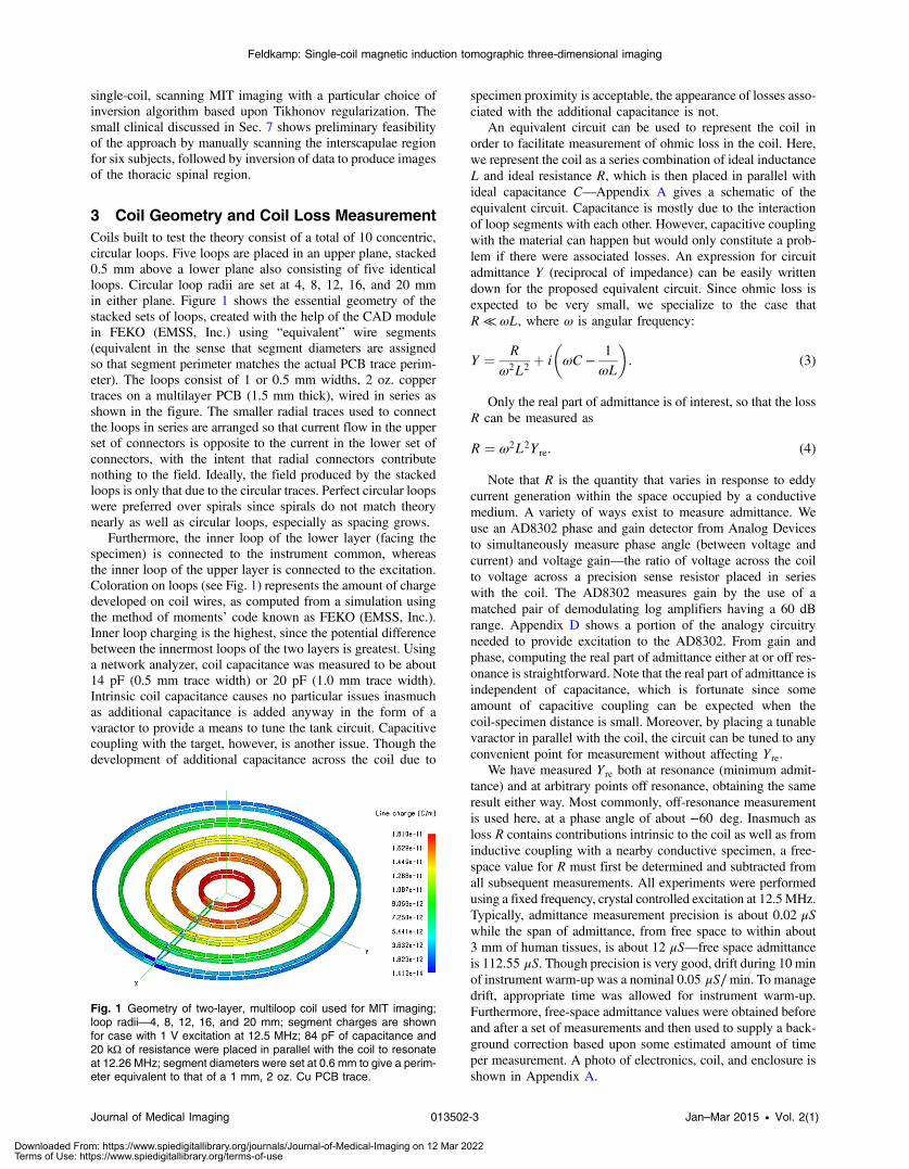
3 Coil Geometry and Coil Loss MeasurementCoils built to test the theory consist of a total of 10 concentric,circular loops. Five loops are placed in an upper plane, stacked0.5 mm above a lower plane also consisting of five identicalloops. Circular loop radii are set at 4, 8, 12, 16, and 20 mmin either plane. Figure 1 shows the essential geometry of thestacked sets of loops, created with the help of the CAD modulein FEKO (EMSS, Inc.) using “equivalent” wire segments(equivalent in the sense that segment diameters are assignedso that segment perimeter matches the actual PCB trace perim-eter). The loops consist of 1 or 0.5 mm widths, 2 oz. coppertraces on a multilayer PCB (1.5 mm thick), wired in series asshown in the figure. The smaller radial traces used to connectthe loops in series are arranged so that current flow in the upperset of connectors is opposite to the current in the lower set ofconnectors, with the intent that radial connectors contributenothing to the field. Ideally, the field produced by the stackedloops is only that due to the circular traces. Perfect circular loopswere preferred over spirals since spirals do not match theorynearly as well as circular loops, especially as spacing grows.

Furthermore, the inner loop of the lower layer (facing thespecimen) is connected to the instrument common, whereasthe inner loop of the upper layer is connected to the excitation.Coloration on loops (see Fig. 1) represents the amount of chargedeveloped on coil wires, as computed from a simulation usingthe method of moments’ code known as FEKO (EMSS, Inc.).Inner loop charging is the highest, since the potential differencebetween the innermost loops of the two layers is greatest. Usinga network analyzer, coil capacitance was measured to be about14 pF (0.5 mm trace width) or 20 pF (1.0 mm trace width).Intrinsic coil capacitance causes no particular issues inasmuchas additional capacitance is added anyway in the form of avaractor to provide a means to tune the tank circuit. Capacitivecoupling with the target, however, is another issue. Though thedevelopment of additional capacitance across the coil due to

specimen proximity is acceptable, the appearance of losses asso-ciated with the additional capacitance is not.

An equivalent circuit can be used to represent the coil inorder to facilitate measurement of ohmic loss in the coil. Here,we represent the coil as a series combination of ideal inductanceL and ideal resistance R, which is then placed in parallel withideal capacitance C—Appendix A gives a schematic of theequivalent circuit. Capacitance is mostly due to the interactionof loop segments with each other. However, capacitive couplingwith the material can happen but would only constitute a prob-lem if there were associated losses. An expression for circuitadmittance Y (reciprocal of impedance) can be easily writtendown for the proposed equivalent circuit. Since ohmic loss isexpected to be very small, we specialize to the case thatR ≪ ωL, where ω is angular frequency:

Y ¼ Rω2L2

þ i

�ωC −

1

ωL

�. (3)

Only the real part of admittance is of interest, so that the lossR can be measured as

R ¼ ω2L2Yre. (4)

Note that R is the quantity that varies in response to eddycurrent generation within the space occupied by a conductivemedium. A variety of ways exist to measure admittance. Weuse an AD8302 phase and gain detector from Analog Devicesto simultaneously measure phase angle (between voltage andcurrent) and voltage gain—the ratio of voltage across the coilto voltage across a precision sense resistor placed in serieswith the coil. The AD8302 measures gain by the use of amatched pair of demodulating log amplifiers having a 60 dBrange. Appendix D shows a portion of the analogy circuitryneeded to provide excitation to the AD8302. From gain andphase, computing the real part of admittance either at or off res-onance is straightforward. Note that the real part of admittance isindependent of capacitance, which is fortunate since someamount of capacitive coupling can be expected when thecoil-specimen distance is small. Moreover, by placing a tunablevaractor in parallel with the coil, the circuit can be tuned to anyconvenient point for measurement without affecting Yre.

We have measured Yre both at resonance (minimum admit-tance) and at arbitrary points off resonance, obtaining the sameresult either way. Most commonly, off-resonance measurementis used here, at a phase angle of about −60 deg. Inasmuch asloss R contains contributions intrinsic to the coil as well as frominductive coupling with a nearby conductive specimen, a free-space value for R must first be determined and subtracted fromall subsequent measurements. All experiments were performedusing a fixed frequency, crystal controlled excitation at 12.5MHz.Typically, admittance measurement precision is about 0.02 μSwhile the span of admittance, from free space to within about3 mm of human tissues, is about 12 μS—free space admittanceis 112.55 μS. Though precision is very good, drift during 10 minof instrument warm-up was a nominal 0.05 μS∕min. To managedrift, appropriate time was allowed for instrument warm-up.Furthermore, free-space admittance values were obtained beforeand after a set of measurements and then used to supply a back-ground correction based upon some estimated amount of timeper measurement. A photo of electronics, coil, and enclosure isshown in Appendix A.

Fig. 1 Geometry of two-layer, multiloop coil used for MIT imaging;loop radii—4, 8, 12, 16, and 20 mm; segment charges are shownfor case with 1 V excitation at 12.5 MHz; 84 pF of capacitance and20 kΩ of resistance were placed in parallel with the coil to resonateat 12.26 MHz; segment diameters were set at 0.6 mm to give a perim-eter equivalent to that of a 1 mm, 2 oz. Cu PCB trace.




To implement Eq. (4), coil inductance is required. For loopsof different radii, the mutual inductance contribution to overallcoil inductance was computed from an equation given byConway,14 rewritten here in a form that uses the zero order,half integer degree toroid function:

Mjk ¼ μffiffiffiffiffiffiffiffiffiρjρk

pQ1∕2

�ρ2j þ ρ2k2ρjρk

�; j ≠ k. (5)

Loop radii are given by ρj and ρk, while magnetic permeabil-ity is given by 1.2566 μH∕m. The toroid function is availablefrom tables or easily computed from a hypergeometric series.If the self-inductance of any individual loop j is given by Lsj,then the mutual inductance between pairs of loops with the sameradius, but in different layers, was just taken to be Lsj—in otherwords, the coupling constant is taken as unity. Self-inductanceof individual loops was computed from simplified equationsgiven by Terman,15 using a “wire” diameter having a circularperimeter equal to the trace perimeter. PCB traces are built ata width of either 1.0 or 0.5 mm using 2 oz. copper, equivalentto about 0.0694 mm thickness. Based upon equivalent perim-eter, a 1.0 mm trace has an equivalent circular wire diameterequal to 0.68 mm and a 0.5-mm trace width has an equivalentdiameter of 0.36 mm. The average of these two is close to0.5 mm, which is the wire diameter used for the inductance cal-culation of either coil. According to the circular loop model,smaller diameter conductors will give a somewhat larger induct-ance, which agrees with network analyzer measurements.Overall, inductance of the 10-loop coil consists of

L ¼X5j¼1

4Lsj þX5j;k¼1

2Mjk; j ≠ k: (6)

Inductance computed in this way was found to be 2.155 μH.Inductance was also measured on an Agilent network analyzer byfirst obtaining the self-resonant frequency of the coil, and then asecond time when placed in parallel with a precision capacitor(�5%). From the two resonant frequencies, L was computedto be 2.132 μH. The uncertainty in the ceramic capacitor, com-bined with the effects of added solder and capacitor leads, on bothinductance and capacitance, makes the network analyzer resultless reliable than the computed inductance—so the latter isused for both coils. However, the difference is only 1% whichvalidates the inductance computation quite well.

4 Comparison of Theory and Experiment for10-Loop Planar Coil

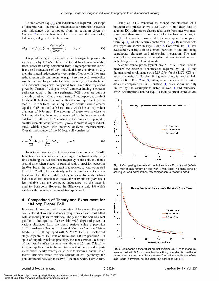
Equation (1) may be used to compute coil loss when the planarcoil is placed at various distances away from a plastic tank filledwith aqueous potassium chloride. The plane of the coil was keptparallel to the liquid surface (within �0.5 deg) and placed atvarious distances from the liquid surface using a precisionXYZ translator (Newport Universal Motion Controller/DriverModel ESP7000; equipped with M-MTM 150 CC1 motorizedstage, capable of 150 mm of travel and 1.0 μm precision). Inspite of superb translator precision, the measurement accuracyof coil-liquid-surface distance was about �0.5 mm. Critical toimaging applications is the requirement that theory and experi-ment match nearly exactly or at least to within a known scalefactor. This was tested for two variants of coil geometry; theonly difference between these two is the trace width, 1 or 0.5 mm.

Using an XYZ translator to change the elevation of amounted coil placed above a 30 × 30 × 13 cm3 deep tank ofaqueous KCl, admittance change relative to free space was mea-sured and then used to compute inductive loss according toEq. (4). This was then compared to the same quantity computedfrom Eq. (1), which is equivalent to R in Eq. (4). Results for bothcoil types are shown in Figs. 2 and 3. Loss from Eq. (1) wasevaluated by using a finite element partition of the tank usingpentahedral elements and nine-point integration. The tankwas only approximately rectangular but was treated as suchin building a finite element mesh.

A conductance probe (sympHony™—VWR) was used tomeasure the electrical conductance required by Eq. (1) andthe measured conductance was 2.86 S∕m for the 1.8% KCl sol-ution (by weight). No data fitting or scaling is used to helpimprove fit in Figs. 2 and 3; rather, experimental and theoreticaldata are compared “as is.” Equation (1) calculations are onlylimited by the assumptions listed in Sec. 1 and numericalerror. Assumptions behind Eq. (1) include small conductivity

Fig. 2 Comparing theoretical predictions from Eq. (1) and (infiniteslab) with measurement on coil with 1 mm trace. No data fitting orscaling is used here; rather, the comparison is “head-to-head.”

Fig. 3 Comparing a theoretical prediction from Eq. (1) with measure-ment on coil with 0.5 mm trace. No data fitting or scaling is used here;rather, the comparison is “head-to-head.” Also included is the infiniteslab result [derivation not included, but similar to Eq. (1)].




and uniform permittivity throughout all space. The latterassumption is not at all met by our system since permittivityabruptly changes at the air-solution interface. But as literatureshows,11,12 lowest order terms developed for the real componentof impedance under nonuniform permittivity conditions [see hisEq. (21)] do not contain permittivity (or, equivalently, speed oflight). Thus, a uniform permittivity approximation is not anissue if only conductivity is of interest. The situation is differentwhen magnetic permeability varies in space, for then the theorybehind Eq. (1) would not be useful for the accurate prediction ofcoil impedance. However, magnetic permeability of humanbody tissues and salt solutions is not significantly differentfrom vacuum. Figures 2 and 3 also contain infinite slab resultsfor a slab having a thickness equal to the finite slab—the infiniteslab equation was derived in a manner similar to Eq. (1) thoughno mesh was needed for calculations.

Results for the narrow trace coil show somewhat betteragreement with theory, which is not surprising since the theorywas developed for infinitely thin conductors. The remaining dis-agreement between theory and experiment arises from severalpossible contributions: (1) coil not perfectly parallel with aque-ous solution interface and vertical positioning accuracy; (2) com-putation/measurement of coil inductance; (3) admittanceaccuracy was judged to be about �0.2 μS, corresponding toa loss error of �0.006 ohm, as computed from Eq. (4); (4) shapeof container holding the KCl solution was not perfectly rectan-gular, and no attempt was made to work with the true containergeometry, which was conceivable but time consuming;(5) numerical errors in computation of loss from Eq. (1)—accu-racy could be improved by refining the mesh used to discretizethe tank; and (6) short range losses due to capacitive couplingwith target—no estimate was made of this. In either Fig. 2 or 3,coil loss is shown to decline substantially when coil-target sep-aration reaches about one coil diameter. However, as Sec. 6shows, the effective range of coil-specimen interaction can beup to five coil diameters when a specimen becomes very large.

5 Inversion Algorithm for Single Coil,Scanning MIT

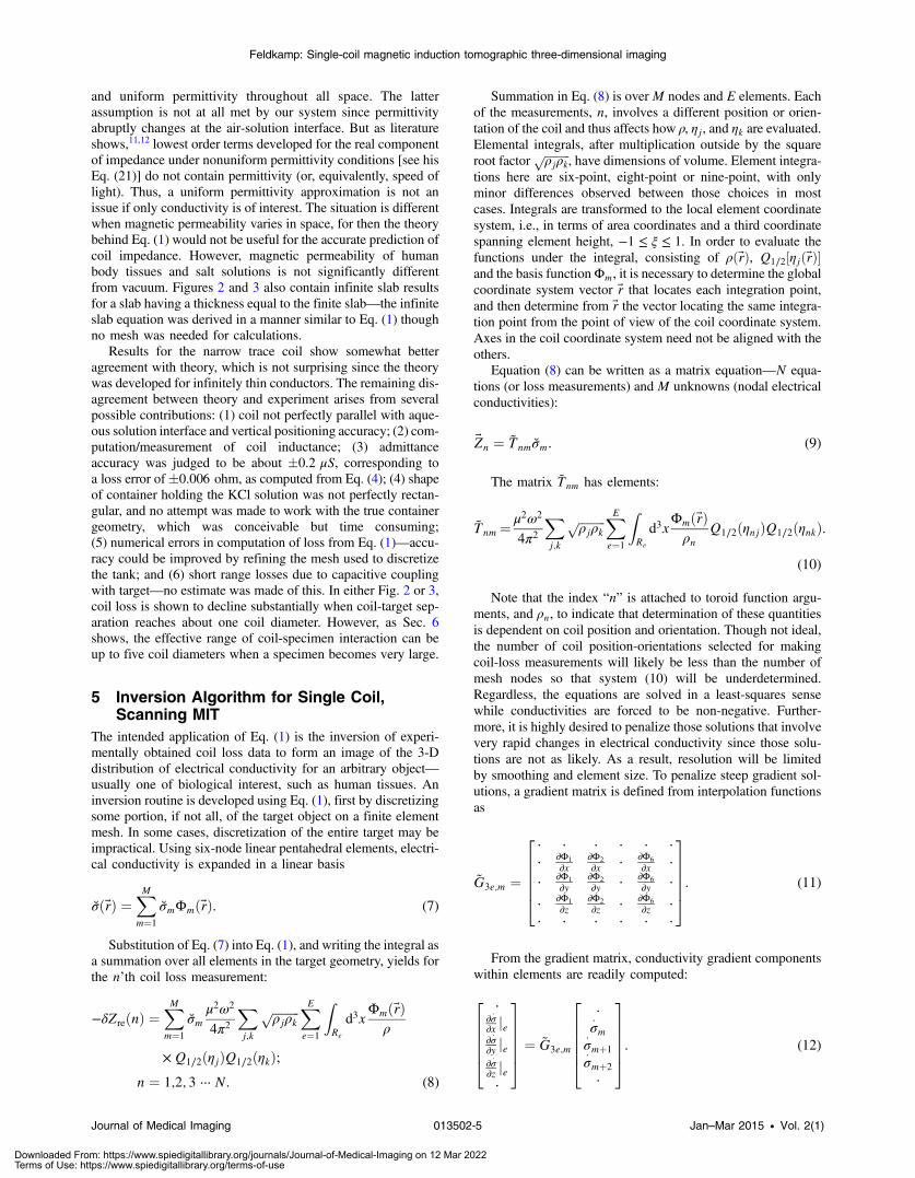
The intended application of Eq. (1) is the inversion of experi-mentally obtained coil loss data to form an image of the 3-Ddistribution of electrical conductivity for an arbitrary object—usually one of biological interest, such as human tissues. Aninversion routine is developed using Eq. (1), first by discretizingsome portion, if not all, of the target object on a finite elementmesh. In some cases, discretization of the entire target may beimpractical. Using six-node linear pentahedral elements, electri-cal conductivity is expanded in a linear basis

σð~rÞ ¼XMm¼1

σmΦmð~rÞ. (7)

Substitution of Eq. (7) into Eq. (1), and writing the integral asa summation over all elements in the target geometry, yields forthe n’th coil loss measurement:

−δZreðnÞ ¼XMm¼1

σmμ2ω2

4π2Xj;k


p XEe¼1

ZRe

d3xΦmð~rÞ

ρ

×Q1∕2ðηjÞQ1∕2ðηkÞ;n ¼ 1;2; 3 ··· N: (8)

Summation in Eq. (8) is overM nodes and E elements. Eachof the measurements, n, involves a different position or orien-tation of the coil and thus affects how ρ, ηj, and ηk are evaluated.Elemental integrals, after multiplication outside by the squareroot factor ffiffiffiffiffiffiffiffiffi

ρjρkp , have dimensions of volume. Element integra-

tions here are six-point, eight-point or nine-point, with onlyminor differences observed between those choices in mostcases. Integrals are transformed to the local element coordinatesystem, i.e., in terms of area coordinates and a third coordinatespanning element height, −1 ≤ ξ ≤ 1. In order to evaluate thefunctions under the integral, consisting of ρð~rÞ, Q1∕2½ηjð~rÞ�and the basis functionΦm, it is necessary to determine the globalcoordinate system vector ~r that locates each integration point,and then determine from ~r the vector locating the same integra-tion point from the point of view of the coil coordinate system.Axes in the coil coordinate system need not be aligned with theothers.

Equation (8) can be written as a matrix equation—N equa-tions (or loss measurements) and M unknowns (nodal electricalconductivities):

~Zn ¼ Tnmσm. (9)

The matrix Tnm has elements:

Tnm ¼ μ2ω2

4π2Xj;k


p XEe¼1

ZRe

d3xΦmð~rÞρn

Q1∕2ðηnjÞQ1∕2ðηnkÞ.

(10)

Note that the index “n” is attached to toroid function argu-ments, and ρn, to indicate that determination of these quantitiesis dependent on coil position and orientation. Though not ideal,the number of coil position-orientations selected for makingcoil-loss measurements will likely be less than the number ofmesh nodes so that system (10) will be underdetermined.Regardless, the equations are solved in a least-squares sensewhile conductivities are forced to be non-negative. Further-more, it is highly desired to penalize those solutions that involvevery rapid changes in electrical conductivity since those solu-tions are not as likely. As a result, resolution will be limitedby smoothing and element size. To penalize steep gradient sol-utions, a gradient matrix is defined from interpolation functionsas

G3e;m ¼

266664

⋅ ⋅ ⋅ ⋅ ⋅ ⋅⋅ ∂Φ1

∂x∂Φ2

∂x ⋅ ∂Φ6

∂x ⋅⋅ ∂Φ1

∂y∂Φ2

∂y ⋅ ∂Φ6

∂y ⋅⋅ ∂Φ1

∂z∂Φ2

∂z ⋅ ∂Φ6

∂z ⋅⋅ ⋅ ⋅ ⋅ ⋅ ⋅

377775. (11)

From the gradient matrix, conductivity gradient componentswithin elements are readily computed:

266664

⋅∂σ⋅

∂x je∂σ⋅

∂y je∂σ⋅

∂z je⋅

377775 ¼ G3e;m

266664

⋅σ⋅m

σ⋅mþ1

σ⋅mþ2

⋅

377775. (12)




To find a set of nodal electrical conductivities that bestexplain the observed coil-loss data, subjected to smoothing,we minimize the two-norm:

k~Zn − Tnmσmk22 þ α2kG3e;mσmk22. (13)

As the smoothing parameter, α, is decreased, the first termbecomes more dominant, thus “sharpening” our focus on anystructure within the conductivity distribution. The approach iswell-known and commonly referred to as Tikhonov regulariza-tion.16 Assignment of α was discussed by Rudnicki andKrawczyk-Stańdo,17 who surveyed a variety of regularizationstrategies, in particular the L-curve method. This approach con-structs a log-log plot of the residual norm against the gradientnorm,16 typically forming an L-shaped curve. Choosing α wherea knee in the L-curve forms has been shown to provide a sat-isfactory compromise between achieving a small residual andadequate smoothing. The method we use here is a close variantof the L-curve approach and is described further in Sec. 7.Minimizing the 2-norm, or Euclidean norm, is equivalent tosolving the following system:

ðTT T þ α2GTGÞσm ≅ TT ~Zn. (14)

Equation (14) is solved with the further constraint that solutioncomponents are non-negative. Ideally, Eq. (14) is sufficient forour needs. However, there are cases where instrumental offsetrelated to drift and aging should be accounted for. This canbe built into Eq. (14) by adding an additional unknown—theinstrument offset, into row one of column vector σm. Thisrequires that a new first column of 1’s be added to the transfer,or translation, matrix ~T. Such a modification will then alsorequire modification of ~G to have a new first row and first col-umn of just zeroes. System (14) is solved with the routineWNNLS (weighted, non-negative least squares), useful onlyfor small to moderate-sized problems (Naval Surface WarfareMath Library). WNNLS is more general than is needed heresince equality constraints could be included. Since equality con-straints are not used, WNNLS is just an NNLS type problem.The strategy for enforcing non-negativity is the so-called activeset method as discussed in Sec. 3.2 of Haskell and Hanson.18

Though there are variants to this method, active and passivesets of unknowns are defined—the former set consisting ofmesh nodes which would violate non-negativity and the latterconsisting of nodes with positive conductivity. Through an iter-ative process described in Sec. 3.2 of their paper, which theystate will always converge, unknowns within the active set trans-fer to the passive set until a solution is eventually found with allnodes satisfying non-negativity.

Because few actual measurements were available per subjectin the study described in Sec. 7, preliminary testing with “virtualmeasurements” was carried out to assess the feasibility of sin-gle-coil MIT imaging with fewer measurements than desired.The next section shows that even with 61 “simulated measure-ments” (132 per subject used in clinical), structures comparablein size with the spinal column and canal can be visualized.

6 Imaging a Prescribed ConductivityDistribution from Simulated Measurements

Because the number of actual measurements per subject in theclinical study was limited, preliminary testing with simulatedmeasurements was carried out to assess the feasibility of

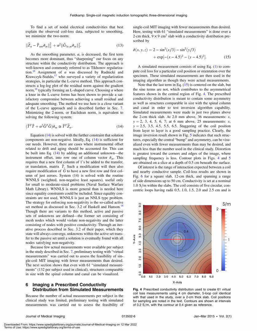
single-coil MIT imaging with fewer measurements than desired.Here, testing with 61 “simulated measurements” is done over a2-cm thick, 9 × 9 cm2 slab with a conductivity distribution pre-scribed by

σðx; y; zÞ ¼ 2 − sin2ðx∕3Þ − sin2ðy∕3Þþ exp½−ðx − 4.5Þ2 − ðy − 4.5Þ2�. (15)

A simulated measurement consists of using Eq. (1) to com-pute coil loss for a particular coil position or orientation over thespecimen. These simulated measurements are then used in theimaging algorithm as though they were actual measurements.

Note that the last term in Eq. (15) is centered on the slab, butthe sine terms are not, which contributes to the asymmetricalfeatures shown in the central region of Fig. 4. The prescribedconductivity distribution is meant to contain some asymmetryas well as structures comparable in size with the spinal columnand canal in order to test inversion algorithm capability.Simulated measurements were made in just two planes abovethe 2-cm thick slab. At 2.0 mm above, 36 measurements: x,y ¼ 2, 3, 4, 5, 6, 7; at 6 mm above, 25 measurements: x,y ¼ 2.5, 3.5, 4.5, 5.5, 6.5. Staggering of the coil positionfrom layer to layer is a good sampling practice. Clearly, theimage inversion result shown in Fig. 5 indicates that such struc-tures, especially the central “bump” and asymmetry, can be visu-alized even with fewer measurements than may be desired, andmuch less than the number used in the clinical study. Distortionis greatest toward the corners and edges of the image, wheresampling frequency is less. Contour plots in Figs. 4 and 5are obtained on a slice at a depth of 0.5 cm beneath the surface.

Of interest is the range of interaction expected between a coiland nearby conductive sample. Coil-loss results are shown inFig. 6 for a square slab, 12-cm thick, and spanning a rangeof side dimensions up to 50 cm. Conductivity is set at a nominal1.0 S∕m within the slabs. The coil consists of five circular, con-centric loops having radii 0.5, 1.0, 1.5, 2.0 and 2.5 cm and is

Fig. 4 Prescribed conductivity distribution used to create 61 virtualcoil loss measurements using 4 cm diameter, 5-loop coil identicalwith that used in the study, over a 2-cm thick slab. Coil positionsfor sampling are noted in the text. Contours are shown at intervalsof 0.2 S∕m, with the contour at 0.4 given as reference.




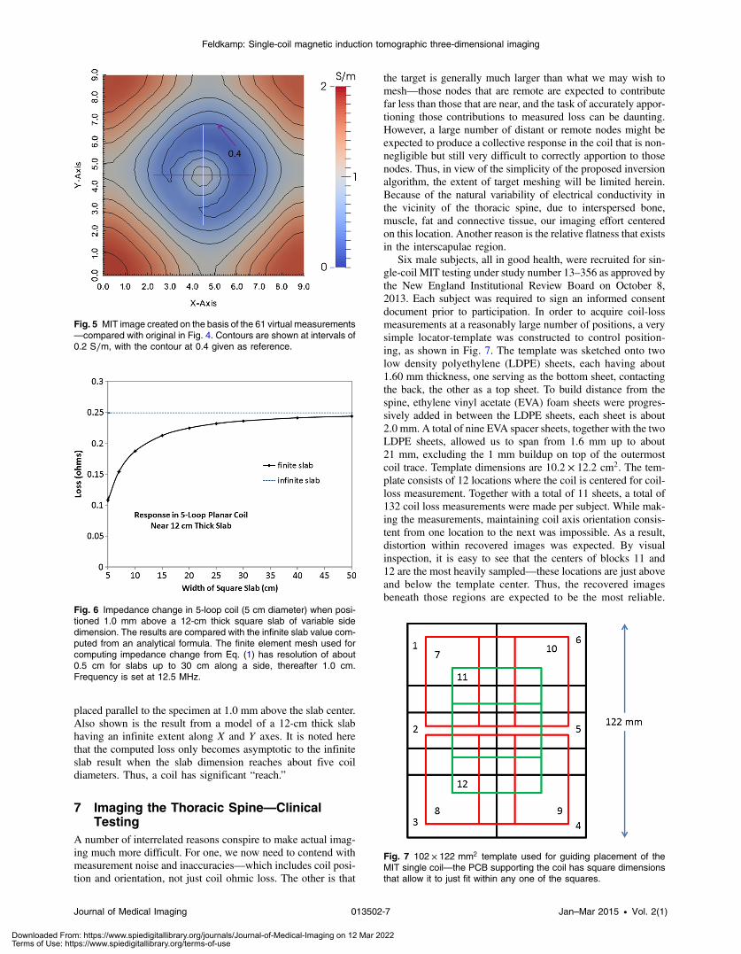
placed parallel to the specimen at 1.0 mm above the slab center.Also shown is the result from a model of a 12-cm thick slabhaving an infinite extent along X and Y axes. It is noted herethat the computed loss only becomes asymptotic to the infiniteslab result when the slab dimension reaches about five coildiameters. Thus, a coil has significant “reach.”

7 Imaging the Thoracic Spine—ClinicalTesting

A number of interrelated reasons conspire to make actual imag-ing much more difficult. For one, we now need to contend withmeasurement noise and inaccuracies—which includes coil posi-tion and orientation, not just coil ohmic loss. The other is that

the target is generally much larger than what we may wish tomesh—those nodes that are remote are expected to contributefar less than those that are near, and the task of accurately appor-tioning those contributions to measured loss can be daunting.However, a large number of distant or remote nodes might beexpected to produce a collective response in the coil that is non-negligible but still very difficult to correctly apportion to thosenodes. Thus, in view of the simplicity of the proposed inversionalgorithm, the extent of target meshing will be limited herein.Because of the natural variability of electrical conductivity inthe vicinity of the thoracic spine, due to interspersed bone,muscle, fat and connective tissue, our imaging effort centeredon this location. Another reason is the relative flatness that existsin the interscapulae region.

Six male subjects, all in good health, were recruited for sin-gle-coil MIT testing under study number 13–356 as approved bythe New England Institutional Review Board on October 8,2013. Each subject was required to sign an informed consentdocument prior to participation. In order to acquire coil-lossmeasurements at a reasonably large number of positions, a verysimple locator-template was constructed to control position-ing, as shown in Fig. 7. The template was sketched onto twolow density polyethylene (LDPE) sheets, each having about1.60 mm thickness, one serving as the bottom sheet, contactingthe back, the other as a top sheet. To build distance from thespine, ethylene vinyl acetate (EVA) foam sheets were progres-sively added in between the LDPE sheets, each sheet is about2.0 mm. A total of nine EVA spacer sheets, together with the twoLDPE sheets, allowed us to span from 1.6 mm up to about21 mm, excluding the 1 mm buildup on top of the outermostcoil trace. Template dimensions are 10.2 × 12.2 cm2. The tem-plate consists of 12 locations where the coil is centered for coil-loss measurement. Together with a total of 11 sheets, a total of132 coil loss measurements were made per subject. While mak-ing the measurements, maintaining coil axis orientation consis-tent from one location to the next was impossible. As a result,distortion within recovered images was expected. By visualinspection, it is easy to see that the centers of blocks 11 and12 are the most heavily sampled—these locations are just aboveand below the template center. Thus, the recovered imagesbeneath those regions are expected to be the most reliable.

Fig. 5 MIT image created on the basis of the 61 virtual measurements—compared with original in Fig. 4. Contours are shown at intervals of0.2 S∕m, with the contour at 0.4 given as reference.

Fig. 6 Impedance change in 5-loop coil (5 cm diameter) when posi-tioned 1.0 mm above a 12-cm thick square slab of variable sidedimension. The results are compared with the infinite slab value com-puted from an analytical formula. The finite element mesh used forcomputing impedance change from Eq. (1) has resolution of about0.5 cm for slabs up to 30 cm along a side, thereafter 1.0 cm.Frequency is set at 12.5 MHz.

Fig. 7 102 × 122 mm2 template used for guiding placement of theMIT single coil—the PCB supporting the coil has square dimensionsthat allow it to just fit within any one of the squares.




Spatial sampling frequency becomes less nearer the outerboundaries of the template so that images are expected to beless reliable there (also noted in virtual tests described in Sec. 6).

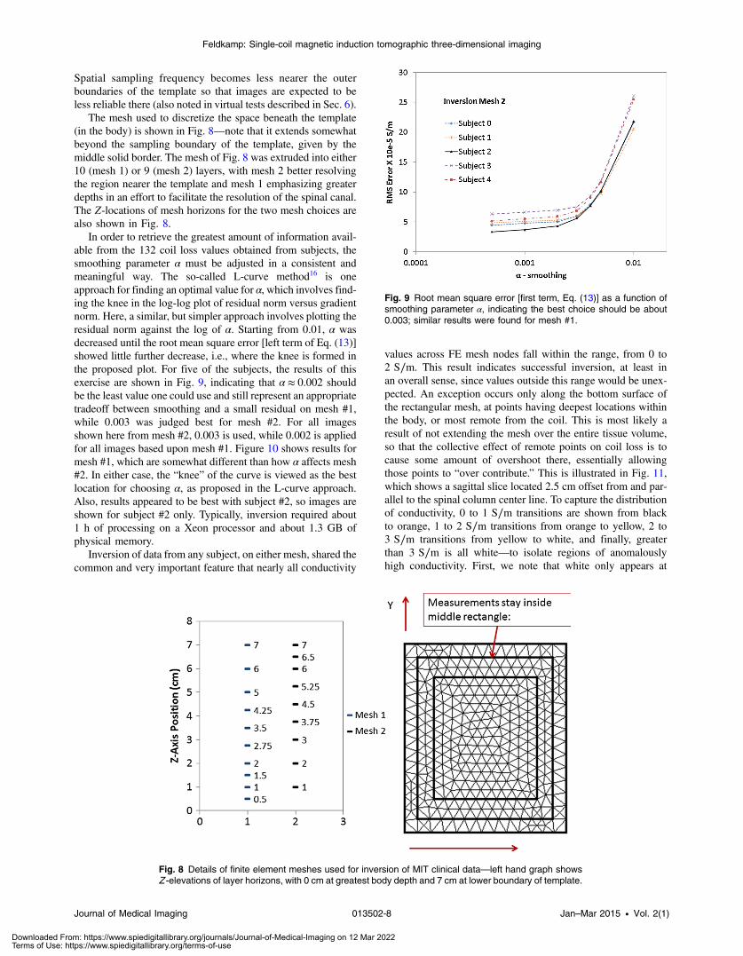
The mesh used to discretize the space beneath the template(in the body) is shown in Fig. 8—note that it extends somewhatbeyond the sampling boundary of the template, given by themiddle solid border. The mesh of Fig. 8 was extruded into either10 (mesh 1) or 9 (mesh 2) layers, with mesh 2 better resolvingthe region nearer the template and mesh 1 emphasizing greaterdepths in an effort to facilitate the resolution of the spinal canal.The Z-locations of mesh horizons for the two mesh choices arealso shown in Fig. 8.

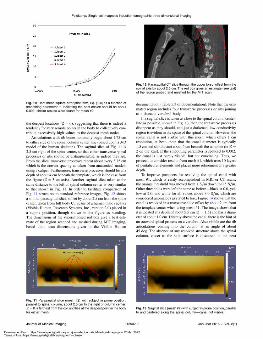
In order to retrieve the greatest amount of information avail-able from the 132 coil loss values obtained from subjects, thesmoothing parameter α must be adjusted in a consistent andmeaningful way. The so-called L-curve method16 is oneapproach for finding an optimal value for α, which involves find-ing the knee in the log-log plot of residual norm versus gradientnorm. Here, a similar, but simpler approach involves plotting theresidual norm against the log of α. Starting from 0.01, α wasdecreased until the root mean square error [left term of Eq. (13)]showed little further decrease, i.e., where the knee is formed inthe proposed plot. For five of the subjects, the results of thisexercise are shown in Fig. 9, indicating that α ≈ 0.002 shouldbe the least value one could use and still represent an appropriatetradeoff between smoothing and a small residual on mesh #1,while 0.003 was judged best for mesh #2. For all imagesshown here from mesh #2, 0.003 is used, while 0.002 is appliedfor all images based upon mesh #1. Figure 10 shows results formesh #1, which are somewhat different than how α affects mesh#2. In either case, the “knee” of the curve is viewed as the bestlocation for choosing α, as proposed in the L-curve approach.Also, results appeared to be best with subject #2, so images areshown for subject #2 only. Typically, inversion required about1 h of processing on a Xeon processor and about 1.3 GB ofphysical memory.

Inversion of data from any subject, on either mesh, shared thecommon and very important feature that nearly all conductivity

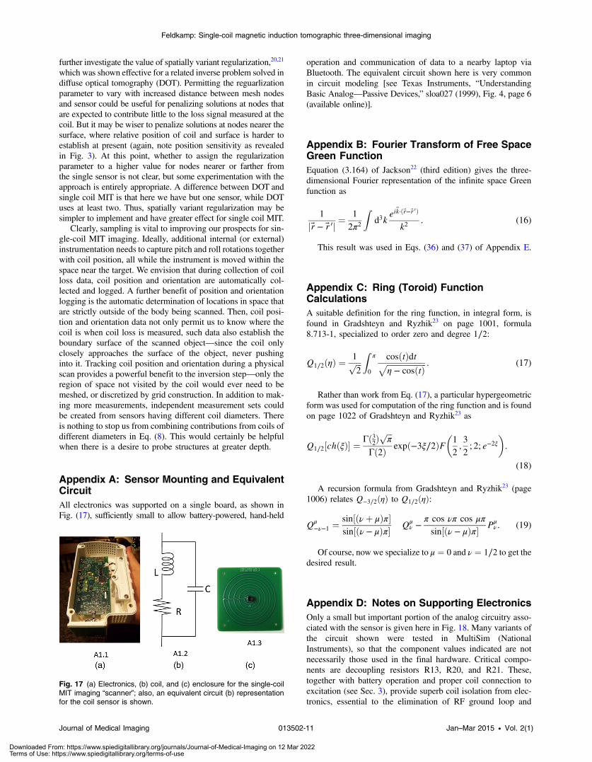
values across FE mesh nodes fall within the range, from 0 to2 S∕m. This result indicates successful inversion, at least inan overall sense, since values outside this range would be unex-pected. An exception occurs only along the bottom surface ofthe rectangular mesh, at points having deepest locations withinthe body, or most remote from the coil. This is most likely aresult of not extending the mesh over the entire tissue volume,so that the collective effect of remote points on coil loss is tocause some amount of overshoot there, essentially allowingthose points to “over contribute.” This is illustrated in Fig. 11,which shows a sagittal slice located 2.5 cm offset from and par-allel to the spinal column center line. To capture the distributionof conductivity, 0 to 1 S∕m transitions are shown from blackto orange, 1 to 2 S∕m transitions from orange to yellow, 2 to3 S∕m transitions from yellow to white, and finally, greaterthan 3 S∕m is all white—to isolate regions of anomalouslyhigh conductivity. First, we note that white only appears at

Fig. 8 Details of finite element meshes used for inversion of MIT clinical data—left hand graph showsZ -elevations of layer horizons, with 0 cm at greatest body depth and 7 cm at lower boundary of template.

Fig. 9 Root mean square error [first term, Eq. (13)] as a function ofsmoothing parameter α, indicating the best choice should be about0.003; similar results were found for mesh #1.




the deepest locations (Z ¼ 0), suggesting that there is indeed atendency for very remote points in the body to collectively con-tribute excessively high values to the deepest mesh nodes.

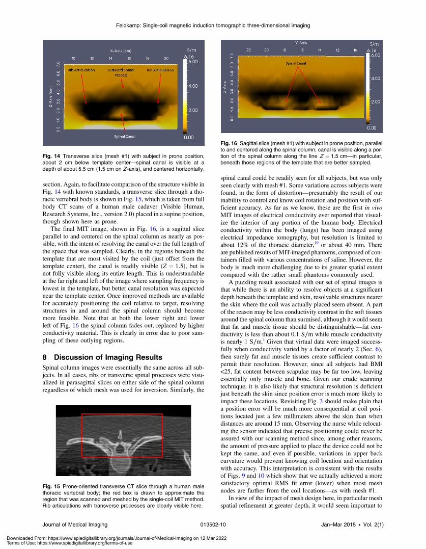
Articulations with rib bones nominally begin about 1.75 cmto either side of the spinal column center line (based upon a 3-Dmodel of the human skeleton). The sagittal slice of Fig. 11 is2.5 cm right of the spine center, so that either transverse spinalprocesses or ribs should be distinguishable, as indeed they are.From the slice, transverse processes repeat about every 3.75 cmwhich is the correct spacing as taken from anatomical modelsusing a caliper. Furthermore, transverse processes should lie at adepth of about 4 cm beneath the template, which is the case fromthe figure (Z ¼ 3 on axis). Another sagittal slice taken at thesame distance to the left of spinal column center is very similarto that shown in Fig. 11. In order to facilitate comparison ofFig. 11 structures to standard reference images, Fig. 12 showsa similar parasagittal slice, offset by about 2.5 cm from the spinecenter, taken from full body CT scans of a human male cadaver(Visible Human, Research Systems, Inc., version 2.0) placed ina supine position, though shown in the figure as standing.The dimensions of the superimposed red box give a best esti-mate of the region scanned and meshed during MIT imaging,based upon scan dimensions given in the Visible Human

documentation (Table 5.3 of documentation). Note that the esti-mated region includes four transverse processes or ribs joiningto a thoracic vertebral body.

If a sagittal slice is taken as close to the spinal column center-line as possible, shown in Fig. 13, then the transverse processesdisappear as they should, and just a darkened, low conductivityregion is evident in the space of the spinal column. However, thespinal canal is not visible with this mesh, which offers 1 cmresolution, at best—note that the canal diameter is typically1.5 cm and should start about 5 cm beneath the template (or Z ¼2 on the axis). If the smoothing parameter is reduced to 0.002,the canal is just barely visible, but not convincing. Thus, weproceed to consider results from mesh #1, which uses 10 layersof pentahedral elements and places more refinement at a greaterdepth.

To improve prospects for resolving the spinal canal withmesh #1, which is easily accomplished in MRI or CT scans,the orange threshold was moved from 1 S∕m down to 0.5 S∕m.Other thresholds were left the same as before—black at 0.0, yel-low at 2.0, and white for all values above 3.0 S∕m, which areconsidered anomalous as stated before. Figure 14 shows that thecanal is resolved in a transverse slice offset by about 2 cm fromthe template center when using mesh #1. The image shows thatit is located at a depth of about 5.5 cm (Z ¼ 1.5) and has a diam-eter of about 1.0 cm. Directly above the canal, there is the hint ofan outward spinal process on a vertebra. Also visible are the ribarticulations coming into the column at an angle of about45 deg. The absence of any resolved structure above the spinalcolumn, closer to the skin surface is discussed in the next

Fig. 10 Root mean square error [first term, Eq. (13)] as a function ofsmoothing parameter α, indicating the best choice should be about0.002; similar results were found for mesh #2.

Fig. 11 Parasagittal slice (mesh #2) with subject in prone position,parallel to spinal column, about 2.5 cm to the right of column center.Z ¼ 0 is farthest from the coil and lies at the deepest point in the bodyfor either mesh.

Fig. 12 Parasagittal CT slice through the upper torso, offset from thespinal axis by about 2.5 cm. The red box gives an estimate (see text)of the region probed and meshed for the MIT scan.

Fig. 13 Sagittal slice (mesh #2) with subject in prone position, parallelto and centered along the spinal column—canal not visible.




section. Again, to facilitate comparison of the structure visible inFig. 14 with known standards, a transverse slice through a tho-racic vertebral body is shown in Fig. 15, which is taken from fullbody CT scans of a human male cadaver (Visible Human,Research Systems, Inc., version 2.0) placed in a supine position,though shown here as prone.

The final MIT image, shown in Fig. 16, is a sagittal sliceparallel to and centered on the spinal column as nearly as pos-sible, with the intent of resolving the canal over the full length ofthe space that was sampled. Clearly, in the regions beneath thetemplate that are most visited by the coil (just offset from thetemplate center), the canal is readily visible (Z ¼ 1.5), but isnot fully visible along its entire length. This is understandableat the far right and left of the image where sampling frequency islowest in the template, but better canal resolution was expectednear the template center. Once improved methods are availablefor accurately positioning the coil relative to target, resolvingstructures in and around the spinal column should becomemore feasible. Note that at both the lower right and lowerleft of Fig. 16 the spinal column fades out, replaced by higherconductivity material. This is clearly in error due to poor sam-pling of these outlying regions.

8 Discussion of Imaging ResultsSpinal column images were essentially the same across all sub-jects. In all cases, ribs or transverse spinal processes were visu-alized in parasagittal slices on either side of the spinal columnregardless of which mesh was used for inversion. Similarly, the

spinal canal could be readily seen for all subjects, but was onlyseen clearly with mesh #1. Some variations across subjects werefound, in the form of distortion—presumably the result of ourinability to control and know coil rotation and position with suf-ficient accuracy. As far as we know, these are the first in vivoMIT images of electrical conductivity ever reported that visual-ize the interior of any portion of the human body. Electricalconductivity within the body (lungs) has been imaged usingelectrical impedance tomography, but resolution is limited toabout 12% of the thoracic diameter,19 or about 40 mm. Thereare published results ofMIT-imaged phantoms, composed of con-tainers filled with various concentrations of saline. However, thebody is much more challenging due to its greater spatial extentcompared with the rather small phantoms commonly used.

A puzzling result associated with our set of spinal images isthat while there is an ability to resolve objects at a significantdepth beneath the template and skin, resolvable structures nearerthe skin where the coil was actually placed seem absent. A partof the reason may be less conductivity contrast in the soft tissuesaround the spinal column than surmised, although it would seemthat fat and muscle tissue should be distinguishable—fat con-ductivity is less than about 0.1 S∕m while muscle conductivityis nearly 1 S∕m.1 Given that virtual data were imaged success-fully when conductivity varied by a factor of nearly 2 (Sec. 6),then surely fat and muscle tissues create sufficient contrast topermit their resolution. However, since all subjects had BMI<25, fat content between scapulae may be far too low, leavingessentially only muscle and bone. Given our crude scanningtechnique, it is also likely that structural resolution is deficientjust beneath the skin since position error is much more likely toimpact these locations. Revisiting Fig. 3 should make plain thata position error will be much more consequential at coil posi-tions located just a few millimeters above the skin than whendistances are around 15 mm. Observing the nurse while relocat-ing the sensor indicated that precise positioning could never beassured with our scanning method since, among other reasons,the amount of pressure applied to place the device could not bekept the same, and even if possible, variations in upper backcurvature would prevent knowing coil location and orientationwith accuracy. This interpretation is consistent with the resultsof Figs. 9 and 10 which show that we actually achieved a moresatisfactory optimal RMS fit error (lower) when most meshnodes are farther from the coil locations—as with mesh #1.

In view of the impact of mesh design here, in particular meshspatial refinement at greater depth, it would seem important to

Fig. 14 Transverse slice (mesh #1) with subject in prone position,about 2 cm below template center—spinal canal is visible at adepth of about 5.5 cm (1.5 cm on Z -axis), and centered horizontally.

Fig. 15 Prone-oriented transverse CT slice through a human malethoracic vertebral body; the red box is drawn to approximate theregion that was scanned and meshed by the single-coil MIT method.Rib articulations with transverse processes are clearly visible here.

Fig. 16 Sagittal slice (mesh #1) with subject in prone position, parallelto and centered along the spinal column; canal is visible along a por-tion of the spinal column along the line Z ¼ 1.5 cm—in particular,beneath those regions of the template that are better sampled.




further investigate the value of spatially variant regularization,20,21

which was shown effective for a related inverse problem solved indiffuse optical tomography (DOT). Permitting the reguarlizationparameter to vary with increased distance between mesh nodesand sensor could be useful for penalizing solutions at nodes thatare expected to contribute little to the loss signal measured at thecoil. But it may be wiser to penalize solutions at nodes nearer thesurface, where relative position of coil and surface is harder toestablish at present (again, note position sensitivity as revealedin Fig. 3). At this point, whether to assign the regularizationparameter to a higher value for nodes nearer or farther fromthe single sensor is not clear, but some experimentation with theapproach is entirely appropriate. A difference between DOT andsingle coil MIT is that here we have but one sensor, while DOTuses at least two. Thus, spatially variant regularization may besimpler to implement and have greater effect for single coil MIT.

Clearly, sampling is vital to improving our prospects for sin-gle-coil MIT imaging. Ideally, additional internal (or external)instrumentation needs to capture pitch and roll rotations togetherwith coil position, all while the instrument is moved within thespace near the target. We envision that during collection of coilloss data, coil position and orientation are automatically col-lected and logged. A further benefit of position and orientationlogging is the automatic determination of locations in space thatare strictly outside of the body being scanned. Then, coil posi-tion and orientation data not only permit us to know where thecoil is when coil loss is measured, such data also establish theboundary surface of the scanned object—since the coil onlyclosely approaches the surface of the object, never pushinginto it. Tracking coil position and orientation during a physicalscan provides a powerful benefit to the inversion step—only theregion of space not visited by the coil would ever need to bemeshed, or discretized by grid construction. In addition to mak-ing more measurements, independent measurement sets couldbe created from sensors having different coil diameters. Thereis nothing to stop us from combining contributions from coils ofdifferent diameters in Eq. (8). This would certainly be helpfulwhen there is a desire to probe structures at greater depth.

Appendix A: Sensor Mounting and EquivalentCircuitAll electronics was supported on a single board, as shown inFig. (17), sufficiently small to allow battery-powered, hand-held

operation and communication of data to a nearby laptop viaBluetooth. The equivalent circuit shown here is very commonin circuit modeling [see Texas Instruments, “UnderstandingBasic Analog—Passive Devices,” sloa027 (1999), Fig. 4, page 6(available online)].

Appendix B: Fourier Transform of Free SpaceGreen FunctionEquation (3.164) of Jackson22 (third edition) gives the three-dimensional Fourier representation of the infinite space Greenfunction as

1

j~r − ~r 0j ¼1

2π2

Zd3k

ei~k·ð~r−~r 0Þ

k2: (16)

This result was used in Eqs. (36) and (37) of Appendix E.

Appendix C: Ring (Toroid) FunctionCalculationsA suitable definition for the ring function, in integral form, isfound in Gradshteyn and Ryzhik23 on page 1001, formula8.713-1, specialized to order zero and degree 1∕2:

Q1∕2ðηÞ ¼1ffiffiffi2

pZ

π

0

cosðtÞdtffiffiffiffiffiffiffiffiffiffiffiffiffiffiffiffiffiffiffiffiη − cosðtÞp : (17)

Rather than work from Eq. (17), a particular hypergeometricform was used for computation of the ring function and is foundon page 1022 of Gradshteyn and Ryzhik23 as

Q1∕2½chðξÞ� ¼Γð3

2Þ ffiffiffi

πp

Γð2Þ expð−3ξ∕2ÞF�1

2;3

2; 2; e−2ξ

�.

(18)

A recursion formula from Gradshteyn and Ryzhik23 (page1006) relates Q−3∕2ðηÞ to Q1∕2ðηÞ:

Qμ−ν−1 ¼

sin½ðνþ μÞπ�sin½ðν − μÞπ� Qμ

ν −π cos νπ cos μπ

sin½ðν − μÞπ� Pμν . (19)

Of course, now we specialize to μ ¼ 0 and ν ¼ 1∕2 to get thedesired result.

Appendix D: Notes on Supporting ElectronicsOnly a small but important portion of the analog circuitry asso-ciated with the sensor is given here in Fig. 18. Many variants ofthe circuit shown were tested in MultiSim (NationalInstruments), so that the component values indicated are notnecessarily those used in the final hardware. Critical compo-nents are decoupling resistors R13, R20, and R21. These,together with battery operation and proper coil connection toexcitation (see Sec. 3), provide superb coil isolation from elec-tronics, essential to the elimination of RF ground loop and

Fig. 17 (a) Electronics, (b) coil, and (c) enclosure for the single-coilMIT imaging “scanner”; also, an equivalent circuit (b) representationfor the coil sensor is shown.




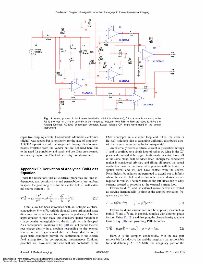
capacitive coupling effects. Considerable additional electronics(digital) was needed but is not shown for the sake of simplicity.AD8302 operation could be supported through developmentboards available from the vendor but are not used here dueto the need for portability and hand-held use. Data are streamedto a nearby laptop via Bluetooth circuitry not shown here.

Appendix E: Derivation of Analytical Coil-LossEquationUnder the restrictions that all electrical properties are time-in-dependent, that permittivity ε and permeability μ are uniformin space, the governing PDE for the electric field ~E 0 with exter-nal source current ~j 0 is

∇2 ~E 0 − εμ∂2 ~E 0

∂t2− μσ

∂~E 0

∂t¼ μ

∂~j 0

∂tþ 1

ε∇ρ 0: (20)

Ohm’s law has been introduced with an isotropic electricalconductivity, σ ¼ σð~rÞ, variable along all three orthogonal spacedirections, and ρ 0 is the electrical space charge density. A furtherapproximation is now made that considers spatial variation incharge density as negligible, so the far right term is dropped.As a consequence, solutions to Eq. (20) will not predict the cor-rect charge density in a medium responding to the externalsource current. Regardless of the true charge distribution, ifquasi-static conditions prevail, the contribution to the electricfield arising from the corresponding instantaneous Coulombpotential will have zero curl and will not contribute to the

EMF developed in a circular loop coil. Thus, the error inEq. (20) solutions due to assuming uniformly distributed elec-trical charge is expected to be inconsequential.

An externally driven electrical current is prescribed through~j 0 and is confined to a single loop of radius ρ0 lying in the XYplane and centered at the origin. Additional concentric loops, allin the same plane, will be added later. Though the conductiveregion is considered arbitrary and filling all space, the actualconductive material encountered in practice will be limited inspatial extent and will not have contact with the source.Nevertheless, boundaries are permitted to extend out to infinitywhere the electric field and its first order spatial derivatives arerequired to vanish. The third term on the left arises due to eddycurrents created in response to the external current loop.

Electric field, ~E 0, and the external source current are treatedas varying harmonically in time at the applied excitation fre-quency ω, so that

~E 0 ¼ ~Eð~rÞe−iωt; ~j 0 ¼ ~jð~rÞe−iωt: (21)

Electric field and current need not be in phase, inasmuch asboth ~Eð~rÞ and ~jð~rÞ are, in general, complex with different phasefactors. Using Eq. (21) and dropping the charge density gradientterm of Eq. (20), our governing PDE becomes

∇2 ~Eþ iωμσ ~E ¼ −iωμ~j; σ ¼ σ − iεω: (22)

Here, σ is the complex conductivity, with the real partresponsible for inductive loss and the imaginary part responsiblefor coil detuning. At 12.5 MHz, the imaginary part of the

Fig. 18 Analog portion of circuit associated with coil (L1 in schematic); C1 is a tunable varactor, whileR2 is the loss in L1—the quantity to be measured; outputs from R15 to R16 are used to drive theAnalog Devices AD8302 phase-gain detector. Lower voltage OP amps were used in the actualinstrument.




conductivity is about 0.07 S∕m if the dielectric constant is 100,which is typical for muscle tissues at this frequency, while 55 istypical for bone and 35 for fat.1 More often, Eq. (22) is written interms of a complex permittivity [see Ref. 24, Eq. (2.32)] ratherthan conductivity when the latter is very small. With the Z-axisnormal to the plane of the coil, only the X and Y components ofthe electric field are needed to compute impedance changes forthe current loop, so it is convenient now to write out the indi-vidual components:

∇2Ex þ iωμσEx ¼ −iωμjx;

∇2Ey þ iωμσEy ¼ −iωμjy.(23)

Using cylindrical coordinates, ρ, ϕ, z, loop current densityhas a contribution only in the angular direction ϕ, equal toJϕ. Thus, the X and Y components of current density can bewritten in terms of cylindrical coordinates as

~j ¼ −Jϕ sin ϕ xþ Jϕ cos ϕ y. (24)

Unit vectors along the X and Y axes are given by x and y.Current density is confined to a loop of wire having an infini-tesimal thickness. Hence, current density Jϕ can be representedin terms of Dirac delta functions:

Jϕ ¼ I0δðzÞδðρ − ρ0Þ. (25)

Using Eqs. (24) and (25), the individual current density com-ponents can be written and then introduced into Eq. (23) to give

∇2Ex þ iωμσEx ¼ iωμI0 sin ϕδðzÞδðρ − ρ0Þ;∇2Ey þ iωμσEy ¼ −iωμI0 cos ϕδðzÞδðρ − ρ0Þ. (26)

A solution is sought after first performing a Fourier transfor-mation of each equation in Eq. (26). For example, the spatialFourier transformation of Exðx; y; zÞ is written as

Exð~kÞ ¼1

ð ffiffiffiffiffi2π

p Þ3Z Z Z

d~rei~k·~rExð~rÞ. (27)

Fourier coordinates are ~k ¼ ðkx; ky; kzÞ and integration isover all Cartesian space. Note there is some flexibility abouthow the Fourier integrals are defined—both regarding the fac-tors of

ffiffiffiffiffi2π

pand the sign of the exponent inside the integrand

(+ or −).25 The Fourier inversion integral is

Exð~rÞ ¼1


p Þ3Z Z Z

d~ke−i~k·~rExð~kÞ. (28)

Similar expressions can be written for the Y-component ofthe electric field.

Fourier transformation is now applied to each of the equa-tions in Eq. (26), leading to

−ðκ2 þ k2zÞEx þiμω


p Þ3Z Z Z

σExei~k·~rd~r

¼ −2πωμI0ρ0ð ffiffiffiffiffi

2πp Þ3

kyκJ1ðκρ0Þ;

−ðκ2 þ k2zÞEy þiμω


p Þ3Z Z Z

σEyei~k·~rd~r

¼ 2πωμI0ρ0ð ffiffiffiffiffi

2πp Þ3

kxκJ1ðκρ0Þ. (29)

As an aid to eventual integration, a cylindrical polar Fouriercoordinate has been defined as κ2 ¼ k2x þ k2y. Far-field boundaryconditions were invoked leading up to Eq. (29), namely thatboth the electric field and its component spatial gradients vanishinfinitely far from the source. Note that there is no near boun-dary or sharp interface between regions, since conductivity istaken as varying continuously throughout all space. Thus,there is no need to invoke the usual boundary conditions on tan-gential and normal fields.

Defining a dimensionless conductivity as Σ ¼ σ∕σ0, with σ0taken as real and nominally 1 S∕m, multiplying Eqs. (29)by ρ20, and defining a dimensionless parameter ξ ¼ μωσ0ρ

20∕


p Þ3, Eqs. (29) can be written as

−ρ20ðκ2 þ k2zÞEx þ iξZ Z Z

ΣExei~k·~rd~r


2πp Þ3

kyκJ1ðκρ0Þ;

−ρ20ðκ2 þ k2zÞEy þ iξZ Z Z

ΣEyei~k·~rd~r


2πp Þ3


At this point, the three-dimensional Fourier convolutiontheorem is needed to cast the remaining integrals solely interms of the Fourier transformed electric field and non-dimen-sional conductivity:Z Z Z

ΣExei~k·~rd~r ¼

Z Z ZΣð~k − ~qÞExð~qÞd~q. (31)

A similar expression can be written for the Y-component ofthe Fourier transformed electric field. Thus, Eq. (30) can bewritten entirely in terms of Fourier transformed field andconductivity:

−ρ20ðκ2 þ k2zÞEx þ iξZ Z Z

Σð~k − ~qÞExð~qÞd~q


2πp Þ3

kyκJ1ðκρ0Þ;

−ρ20ðκ2 þ k2zÞEy þ iξZ Z Z

Σð~k − ~qÞEyð~qÞd~q


2πp Þ3


Because the non-dimensional real parameter ξ is very small(≪1), a regular perturbation solution approach is useful. Thus,expansions in ξ are prepared in the form:




Ex ¼X∞n¼0

Exnξn; Ey ¼

X∞n¼0

Eynξn. (33)

If these expansions are inserted into Eq. (32), with terms hav-ing like powers of ξ gathered together, a sequence of solutions isrecovered. The zero-order solutions are

Ex0 ¼ 2πωμI0ρ0ð ffiffiffiffiffi

2πp Þ3

kyκðκ2 þ k2zÞ

J1ðκρ0Þ;

Ey0 ¼ −2πωμI0ρ0ð ffiffiffiffiffi

2πp Þ3

kxκðκ2 þ k2zÞ

J1ðκρ0Þ. (34)

These may be inverted and further developed to yield thewell-known solution for the magnetic vector potential for a cir-cular current loop in free space in the quasi-static limit (Panofskyand Phillips,26 second edition, page 156, obtained using a sepa-ration of variables approach). We proceed to get first order sol-utions from the zero-order solutions:

Ex1 ¼iR R R

Σð~k − ~qÞExoð~qÞd~qρ20ðκ2 þ k2zÞ

;

Ey1 ¼iR R R

Σð~k − ~qÞEyoð~qÞd~qρ20ðκ2 þ k2zÞ

. (35)

After first substituting the Fourier transformed electrical con-ductivity, Σ, followed by introduction of zero-order solutions, allFourier integrations involving ~qmay be completed. This leads toX and Y components for the first order solutions to the electricfield in Fourier space:

Ex1ð~kÞ ¼ωμI02πρ0

Z Z Zd~rΣð~rÞ sin ϕffiffiffiffiffiffiffi

ρρ0p Q1∕2ðηÞ

ei~k·~r

k2;

η ¼ ρ2 þ ρ20 þ z2

2ρρ0(36)

and

Ey1ð~kÞ ¼ −ωμI02πρ0

Z Z Zd~rΣð~rÞ cos ϕffiffiffiffiffiffiffi

ρρ0p Q1∕2ðηÞ

ei~k·~r

k2.

(37)

Note that the argument of the toroid (or ring) functionQ1∕2ðηÞ lies in the interval 1 < η < ∞, and is readily evaluatedusing the hypergeometric series form (Appendix C). Equa-tions (36) and (37) are straightforward to invert, giving firstorder components of the electric field in Cartesian space. UsingEq. (3.164) of Jackson22 (third edition—see Appendix B) andreturning to dimensioned electrical conductivity:

Ex1ð~rÞ ¼ωμI0

σ0ρ0ffiffiffiffiffi8π

pZ Z Z

d~r 0σð~r 0Þ sin ϕ 0ffiffiffiffiffiffiffiffiffiρ 0ρ0

p Q1∕2ðη 0Þj~r − ~r 0j

(38)

and

Ey1ð~rÞ ¼ −ωμI0

σ0ρ0ffiffiffiffiffi8π

pZ Z Z

d~r 0σð~r 0Þ cos ϕ0ffiffiffiffiffiffiffiffiffi

ρ 0ρ0p Q1∕2ðη 0Þ

j~r − ~r 0j .

(39)

Equations (38) and (39) lead to corrections for the electricfield after multiplying by ξ:

δExð~rÞ ¼μ2ω2ρ0I0

8π2

Z Z Zd~r 0σð~r 0Þ sin ϕ 0ffiffiffiffiffiffiffiffiffi

ρ 0ρ0p Q1∕2ðη 0Þ

j~r − ~r 0j ;

(40)

and for the Y-component,

δEyð~rÞ ¼ −μ2ω2ρ0I0

8π2

Z Z Zd~r 0σð~r 0Þ cos ϕ

0ffiffiffiffiffiffiffiffiffiρ 0ρ0

p Q1∕2ðη 0Þj~r − ~r 0j .

(41)

The impedance change for a single loop, in response to coil-target interaction, is given by integration of the electric fieldalong the circular loop:

δZ ¼ 1

I0

Iδ~E · d~r

¼ 1

I0

Z2π

0

ð−δEx sin ϕþ δEy cos ϕÞρ0dϕ. (42)

An expansion for the free space Green function in Eqs. (40)or (41), in cylindrical coordinates, greatly facilitates completingthe integrals in Eq. (42) and is found in Cohl et al.27

1

j~r − ~r 0j ¼1

πffiffiffiffiffiffiffiρρ 0p X∞

m¼−∞Qm−1∕2ðηÞeimðϕ−ϕ 0Þ;

η ≡ρ2 þ ρ 02 þ ðz − z 0Þ2

2ρρ 0 . (43)

Substitution of Eq. (43) into Eqs. (40) and (41) and then plac-ing the results into Eq. (42) leads to the desired impedancechange for a coil fashioned from a single loop:

δZ ¼ −μ2ω2ρ04π2

Zd3x

σð~rÞρ

½Q1∕2ðηÞ�2;

η ≡ρ20 þ ρ2 þ z2

2ρρ0. (44)

Equation (44) is obtained by noting that contributions fromthe sum in Eq. (43) come only from m ¼ �1; and making useof a recursion formula given in Gradshteyn and Ryzhik,23 page1006, Appendix C shows that Q−3∕2ðηÞ ¼ Q1∕2ðηÞ. Inasmuchas electrical conductivity is complex valued, we have both realand imaginary components for impedance change in the loop:

δZre ¼ −μ2ω2ρ04π2

Zd3x

σð~rÞρ

½Q1∕2ðηÞ�2;

δZim ¼ εμ2ω3ρ04π2

Zd3x

½Q1∕2ðηÞ�2ρ

.

(45)

Though electrical conductivity does not appear in the imagi-nary component of impedance change, there is nonetheless an




impedance change, but it is not really caused by the conductivetarget. Rather, the imaginary component arises as a correctiondue to the finite speed of light, coming from the first order per-turbation correction. In fact, had the middle term on the left handside of Eq. (20) been dropped at the outset, as is usually done toapproximate light travel as instantaneous, then the imaginarycomponent would be absent here. Indeed, as is shown byHarpen11 for the simpler case of a conductive sphere in a spa-tially uniform RF field, the real part of impedance change variesas the square of frequency while the imaginary part varies as thecube of frequency [see Eqs. (21) and (22)]. Furthermore, hisresult shows a first order correction to the real component ofimpedance varying linearly with conductivity, and the firstorder correction to the imaginary component as independentof conductivity. All terms appearing in his expansion of thereal component of impedance change are independent of permit-tivity. Harpen’s paper also gives important experimental resultsfor conductive spheres (radius ¼ 4.5 cm) showing that the realpart of impedance varies linearly with conductivity up to2.0 S∕m at a frequency of 63 MHz and then begins to tailoff due to skin depth effects. He also showed third powerdependence on frequency for the imaginary impedance compo-nent up to 90 MHz for low conductivity media. Thus, to avoidskin depth effects, experimental work is conducted here at12.5 MHz, well below the 63 MHz threshold given by Harpen.

Results thus far pertain to the case of a single circular loopcentered at the origin and lying in the XY-plane. This can beextended to treat the case of any number of circular concentricloops all centered at the origin and lying within the XY-plane—the loops are presumed wired in series and carrying the samecurrent, I0. For a specific loop of radius ρj, Eqs. (40) and(41) are rewritten:

δExð~rÞ ¼μ2ω2ρjI0

8π2

Z Z Zd~r 0σð~r 0Þ sin ϕ 0ffiffiffiffiffiffiffiffiffi

ρ 0ρjp Q1∕2ðη 0

jÞj~r − ~r 0j ;

(46)

δEyð~rÞ ¼ −μ2ω2ρjI0

8π2

Z Z Zd~r 0σð~r 0Þ cos ϕ

0ffiffiffiffiffiffiffiffiffiρ 0ρj

p Q1∕2ðη 0jÞ

j~r − ~r 0j .

(47)

The magnetic flux from loop j links every other loop, includ-ing itself. Specifically, flux from loop j linking loop k producesa contribution to impedance change for the collection of loops inseries:

δZk ¼1

I0

Iδ~E · d~r

¼ ρkI0

Z2π

0

ð−δEx sin ϕþ δEy cos ϕÞdϕ. (48)

Introducing the changes in the electric field into Eq. (48) leadto the real component of impedance change:

δZreðjkÞ ¼ −μ2ω2 ffiffiffiffiffiffiffiffiffi

ρjρkp4π2

Zd3x

σð~rÞρ

Q1∕2ðηjÞQ1∕2ðηkÞ;(49)

where

ηj ¼ρ2 þ ρ2j þ z2

2ρρj; ηk ¼

ρ2 þ ρ2k þ z2

2ρρk. (50)

Total impedance change is then given by a double summa-tion, allowing for contributions due to any loop interacting withany other loop as well as itself:

δZre ¼ −μ2ω2

4π2Xj;k


p Zd3x

σð~rÞρ

Q1∕2ðηjÞQ1∕2ðηkÞ.

(51)

In the experimental sections, we compare this multilooptheoretical result with experimental coil measurements overan aqueous potassium chloride solution and then go on to exper-imentally demonstrate its great utility for single coil MIT imag-ing of the upper thoracic spine where natural conductivitycontrasts are expected due to bone and muscle tissues.

AcknowledgmentsConstruction of electronics and enclosure for MIT measure-ments by Plexus Services Corporation in Neenah, Wisconsin,is gratefully acknowledged. Also, we wish to thank the ClinicalResearch Services team at Kimberly-Clark Corporation for as-sistance with the clinical study.

References1. C. Gabriel, S. Gabriel, and E. Courthout, “The dielectric properties of

biological tissues: I. Literature survey,” Phys. Med. Biol. 41, 2231–2249(1996).

2. D. Haemmerich et al., “In vivo electrical conductivity of hepatictumors,” Physiol. Meas. 24, 251–260 (2003).

3. J. Songer, “Tissue ischemia monitoring using impedance spectroscopy:clinical evaluation,” M.S. Thesis, Worcester Polytechnic Institute(2001).

4. H. Y. Wei and M. Soleimani, “Electromagnetic tomography for medicaland industrial applications: challenges and opportunities,” Proc. IEEE101, 559–564 (2013).

5. T. M. Taves and S. B. King, “In vivo conductivity measurement usingMRI based noise tomography at 3T,” in Proc. Joint Annual Meeting ofISMRM-ESMRMB, p. 331, Berlin, Germany (2007).

6. E. C. Herrman et al., “Skin perfusion responses to surface pressure-induced ischemia: implication for the developing pressure ulcer,” J.Rehabil. Res. Dev. 36(2), 109–120 (1999).

7. J. R. Feldkamp and J. Heller, “Effects of extremity elevation and healthfactors on soft tissue electrical conductivity,”Meas. Sci. Rev. 9(6), 169–178 (2009).

8. H. Y. Wei and M. Soleimani, “Three dimensional magnetic inductiontomography imaging using a matrix free Krylov subspace inversionalgorithm,” Prog. Electromagn. Res. 122, 29–45 (2012).

9. H. Scharfetter et al., “Single-step 3D image reconstruction in magneticinduction tomography: theoretical limits of spatial resolution and con-trast to noise ratio,” Ann. Biomed. Eng. 34, 1786–1798 (2006).

10. C. H. Igney, R. Pinter, and O. Such, “Magnetic induction tomographysystem and method,” U.S. Patent No. 8,125,220 B2 (2012).

11. M. D. Harpen, “Influence of skin depth on NMR coil impedance: PartII,” Phys. Med. Biol. 33, 597–605 (1988).

12. M. D. Harpen, “Distributed self-capacitance of magnetic resonance sur-face coils,” Phys. Med. Biol. 33, 1007–1016 (1988).

13. A. J. M. Zaman, S. A. Long, and C. G. Gardner, “The impedance of asingle-turn coil near a conducting half space,” J. Nondestructive Eval.1(3), 183–189 (1980).

14. J. T. Conway, “Inductance calculations for non-coaxial coils usingBessel functions,” IEEE Trans. Magn. 43, 1023–1034 (2007).

15. F. E. Terman, Radio Engineer’s Handbook, 1st ed., McGraw-Hill,London (1950).




http://dx.doi.org/10.1088/0031-9155/41/11/001

http://dx.doi.org/10.1088/0967-3334/24/2/302

http://dx.doi.org/10.1109/JPROC.2012.2237072

http://dx.doi.org/10.2478/v10048-009-0028-0

http://dx.doi.org/10.2528/PIER11091513

http://dx.doi.org/10.1007/s10439-006-9177-6

http://dx.doi.org/10.1088/0031-9155/33/5/007

http://dx.doi.org/10.1088/0031-9155/33/9/001

http://dx.doi.org/10.1007/BF00567090

http://dx.doi.org/10.1109/TMAG.2006.888565

16. Å. Björck, Numerical Methods for Least Squares Problems, Vol. 204,p. 204, Society for Industrial and Applied Mathematics, Philadelphia(1996).

17. M. Rudnicki and D. Krawczyk-Stańdo, “Modern regularization tech-niques for inverse modelling: a comparative study,” in X-thInternational Workshop on Optimization and Inverse Problems inElectromagnetism, Sept. 14-17, pp. 56–59, Ilmenau, Germany (2008).

18. K. H. Haskell and R. J. Hanson, “An algorithm for linear least squaresproblems with equality and nonnegativity constraints,”Math. Program.21, 98–118 (1981).

19. E. L. V. Costa, R. G. Lima, and M. B. P. Amato, “Electrical impedancetomography,” Curr. Opin. Crit. Care 15, 18–24 (2009).

20. H. Dehghani et al., “Depth sensitivity and image reconstruction analysisof dense imaging arrays for mapping brain function with diffuse opticaltomography,” Appl. Opt. 48(10), D137–D143 (2009).

21. S. H. Katamreddy and P. K. Yalavarthy, “Model-resolution based regu-larization improves near infrared diffuse optical tomography,” J. Opt.Soc. Am. 29(5), 649–656 (2012).

22. J. D. Jackson, Classical Electrodynamics, 3rd ed., JohnWiley and Sons,New York, NY (1999).

23. I. S. Gradshteyn and Ryzhik, “Table of integrals, series and products,”Corrected and Enlarged Edition, A. Jeffrey, Academic Press, NewYork, NY (1980).

24. L. Novotny and B. Hecht, Principles of Nano-Optics, 2nd ed.,Cambridge University Press, Cambridge, UK (2012).

25. E. Zauderer, Partial Differential Equations of Applied Mathematics,John Wiley & Sons, Inc., New York, NY (1983).

26. W. K. H. Panofsky and M. Phillips, Classical Electricity andMagnetism, 2nd ed., Addison-Wesley Publ. Co., Reading,Massachusetts(1962).

27. H. S. Cohl et al., “Developments in determining the gravitational poten-tial using toroidal functions,” Astron. Nachr. 321, 363–372 (2000).

Joseph R. Feldkamp is a physical scientist, with MS and PhDdegrees from Purdue University. He has been a research technicalleader at Kimberly-Clark for nearly 15 years. Previous positionswere held at Diconix, Monsanto, Northwestern University andApplied Research Associates. His current research interests includeapplications of electrodynamics to the development of biologicalsensors.




http://dx.doi.org/10.1007/BF01584232

http://dx.doi.org/10.1097/MCC.0b013e3283220e8c

http://dx.doi.org/10.1364/AO.48.00D137

http://dx.doi.org/10.1364/JOSAA.29.000649

http://dx.doi.org/10.1364/JOSAA.29.000649

http://dx.doi.org/10.1002/(ISSN)1521-3994

single-coil magnetic induction tomographic three

Documents