shankar jfm thermal

8/11/2019 Shankar Jfm Thermal

http://slidepdf.com/reader/full/shankar-jfm-thermal 1/26

J. Fluid Mech. (2008), vol. 605, pp. 329–354. c 2008 Cambridge University Pressdoi:10.1017/S0022112008001468 Printed in the United Kingdom

329

Numerical simulation of the uid dynamic effectsof laser energy deposition in air

S H A N K A R G H O S H AND K R I S H N A N M A H E S HAerospace Engineering and Mechanics, University of Minnesota, MN 55455, USA

(Received 8 June 2006 and in revised form 6 March 2008)

Numerical simulations of laser energy deposition in air are conducted. Localthermodynamic equilibrium conditions are assumed to apply. Variation of thethermodynamic and transport properties with temperature and pressure are accountedfor. The ow eld is classied into three phases: shock formation; shock propagation;and subsequent collapse of the plasma core. Each phase is studied in detail. Vorticitygeneration in the ow is described for short and long times. At short times, vorticityis found to be generated by baroclinic means. At longer times, a reverse ow is foundto be generated along the plasma axis resulting in the rolling up of the ow eld nearthe plasma core and enhancement of the vorticity eld. Scaling analysis is performedfor different amounts of laser energy deposited and different Reynolds numbers of the ow. Simulations are conducted using three different models for air based ondifferent levels of physical complexity. The impact of these models on the evolutionof the ow eld is discussed.

1. IntroductionThe deposition of laser energy into air has been studied by a number of workers

(e.g. Damon & Tomlinson 1963; Knight 2003; Maker, Terhune & Savage 1963;Meyerand & Haught 1963; Root 1989), and nds application in localized owcontrol of supersonic ows (Adelgren et al. 2003; Shneider et al. 2003), drag reductionin supersonic and hypersonic ows (Riggins, Nelson & Johnson 1999), ignition of combustion gases (Phuoc 2000) and provision of thrust to aerospace vehicles (Molina-Morales et al. 2001; Wang et al. 2001). When a laser beam is focused on a smallvolume of gas, the gas molecules in the focal volume absorb energy and are ionized.A simple description of the plasma formation process is as follows (Raizer 1966;Morgan 1975; Keefer 1989; Phuoc 2005). Electrons are initially released owing tomulti-photon ionization, when multiple photons are simultaneously incident on anatom. During this process, the electron number density increases linearly in time. Thereleased electrons absorb laser energy owing to inverse bremsstrahlung absorption,where a free electron in the presence of a third body absorbs energy and becomesexcited. After many such interactions, the electron gains sufficient energy to impact-ionize neutral atoms. The electron concentration then increases exponentially in time.The resulting plasma reects part of the incident laser energy. This energy is absorbedby adjacent molecules along the laser axis in the direction of the laser source. These

molecules then become ionized, and start reecting laser radiation. This processcontinues until the plasma evolves into a tear-drop shape. The collision of energeticelectrons with heavy particles results in heating of the gas. Also, the electron numberdensity decreases owing to recombination of the electrons with ions. A region where



330 S. Ghosh and K. Mahesh

temperature and pressure are higher than that of the surroundings is obtained atthe end of plasma formation. The resulting pressure gradients lead to formation of ablast wave that propagates into the background gas.

Recent experiments on pulsed laser-induced breakdown include Jiang et al. (1998),Lewis et al. (1999), Adelgren, Boguszko & Elliott (2001) and Glumac, Elliott &Boguszko (2005 a,b). Jiang et al. (1998) focused a laser beam of 1 .38 J on a 3 mmdiameter spherical region to cause breakdown of air. The laser was pulsed for aduration of 18 ns. Adelgren et al. (2001) pulsed a Nd:YAG laser of 200mJ for 10 nsin air. The experimental data show a wide separation in time scales between laserpulse duration and blast wave propagation, i.e. the laser is pulsed on a time scaleof 10 ns while the blast wave is observed on a time scale of 10 to 100 µ s. Since theplasma forms on the time scale of the laser pulse duration, there is a three to fourorder of magnitude separation in time scale. The plasma may therefore be assumedto form instantaneously, to evaluate its gas-dynamic effect on the surrounding uid.

Various simulation models have been used to understand different features of this

phenomenon. Brode (1955) numerically simulated the blast wave and concluded thatthe ideal gas assumption was reasonable for shock pressures of less than 10 atm inair. Steiner, Gretlef & Hirschler (1998) perform computations using a real-gas modelto show that when initialized with a self-similar strong-shock solution, the shockradius in the real-gas model is quite close to that predicted by the classical point-source explosion in an ideal gas. Other computations of blast-wave propagationin quiescent air include those by Jiang et al. (1998) and Yan et al. (2003). Dors,Parigger & Lewis (2000) and Dors & Parigger (2003) present a computational modelwhich considers the asymmetry of laser energy deposition as well as ionization anddissociation effects on uid properties. The initial stages of plasma formation due tolaser energy deposition were modelled by Kandala & Candler (2003) and Kandalaet al . (2005). Very few simulations account for the physical tear-drop shape of theplasma. Even simulations with complex physical models do not show the prominentow features observed in experiment. One of the objectives of this paper is toinvestigate the level of physical complexity required to simulate accurately the owfeatures observed in the experiments. This paper considers generation of laser-inducedplasma in quiescent air. Local thermodynamic equilibrium conditions are assumed toapply. The simulations are conducted using three different models for air based ondifferent levels of physical complexity. Figure 1 shows a schematic of the problem.The relevant parameters associated with the problem are the shape and size of theinitial plasma region, the maximum temperature ratio in the plasma core T 0 andviscosity of the uid. The time evolution of the resulting ow eld is divided intoshock formation, shock propagation and subsequent roll-up of the plasma core. Eachstage is discussed in detail. An explanation of the process of the rolling up of theplasma core is provided. Vorticity is found to be generated at short and long timesthrough different mechanisms. At short times, vorticity generated in the ow is dueto baroclinic production whereas at long times, vorticity is generated owing to rollingup of the plasma core. These mechanisms are studied in detail. Scaling analysis isperformed for different values of T 0 and the Reynolds number of the ow. A Fourierspectral solver is developed for conducting the simulations. Numerical challengesassociated with the simulations are discussed in detail.

This paper is organized as follows. Section 2 discusses the primary numericalchallenges posed by the ow, and describes the numerical methodology. Simulationresults are discussed in §3. Section 3.1 starts with an overview of the ow eld andthen proceeds to describe the ow in each of the three phases of shock formation,



Numerical simulation of uid dynamic effects of laser energy deposition in air 331

Laser Plasmaformation

Shock formation

Shock propagation

Rollup

Figure 1. Schematic showing stages involved in laser-induced breakdown of a gas.

propagation and collapse of the core. The evolution of velocity, temperature andvorticity are discussed. The effect of maximum initial core temperature T 0 andReynolds number on the ow is discussed in §3.2. Section 3.3 shows simulationresults from three different models used for air. A short summary in §4 concludes thepaper.

2. Simulation methodology2.1. Governing equations

The Navier–Stokes equations are used to simulate the ow eld resulting from thedeposition of laser energy in air. Local thermodynamic equilibrium conditions areassumed to apply. Also, radiation losses after formation of the plasma spot areassumed to be negligible. Hence, the governing equations do not have additionalsource terms. The continuity, and compressible Navier–Stokes equations are given by

∂ρ∂t

+ ∂ρu i

∂x i= 0 , (2.1)

∂ρu j

∂t +

∂ρu j u i

∂x i= −

∂∂x i

pδ ij − µRe

∂u i

∂x j +

∂u j

∂x i−

23

∂u k

∂xkδij , (2.2)

∂ρe T

∂t + ∂ρe T u i

∂x i= ∂

∂x i− pu i + µ

Re∂u i

∂x j + ∂u j

∂x i− 2

3∂u k

∂xkδij u j

+ ∂∂x i

κ(γ − 1)RePr

∂T ∂x i

(2.3)

where all the variables are non-dimensionalized by their initial background values.

x i = x∗i /L∗

0, u i = u∗i /c ∗0 , t = t ∗c∗0/L ∗

0,

ρ = ρ∗/ρ ∗

0 , p = p ∗/ρ ∗

0 c∗02, T = T ∗/T ∗0

µ = µ∗/µ ∗

0, κ = κ∗/κ ∗

0 .

(2.4)

Here, the subscript ‘0’ denotes initial background values and the superscript, asteriskdenotes dimensional variables. L∗0 is the reference length scale and is obtained bycomparing the non-dimensional length of the plasma region used in the simulations




to the physical length of the plasma. c∗0 is the speed of sound based on initialbackground temperature; i.e.

c∗0 = ( γ R ∗T ∗0 )1/ 2. (2.5)The Reynolds number and Prandtl number are dened as

Re = ρ∗0 c∗0L∗0/µ ∗0, P r = µ ∗c∗p /k ∗. (2.6)

Simulations are conducted using models with three different levels of physicalcomplexity. These models are described below.

2.1.1. Model 1For the simplest case (model 1), the effects of chemical reactions resulting from

high temperatures in the ow are neglected. Ideal-gas relations are used to representthe thermodynamic properties of air. Simple constitutive relations are assumed forthe transport properties. The coefficient of viscosity is described by the power law

µ = T 0.67, (2.7)

the coefficient of thermal conductivity is obtained by assuming a constant Prandtlnumber of 0 .7, and γ is assumed to be 1 .4. The non-dimensionalized equation of state becomes

p = ρT/γ, (2.8)where the temperature is related to the internal energy by the relation

T = γ (γ − 1)e, (2.9)

and the total energy is related to internal energy and kinetic energy asρe T = ρe + 1

2 ρu i u i . (2.10)

To obtain the initial conditions, a three-dimensional temperature prole is used torepresent the heating effect of laser energy deposition. Since the energy addition is ona very fast time scale, the density is assumed constant. The initial pressure prole isthen obtained using (2.15) and the internal energy e is obtained using (2.9). At theend of every time step, pressure and temperature are obtained from the conservedvariables using the above constitutive equations.

2.1.2. Model 2Model 2 considers the effect of chemical reactions resulting in dissociation,

ionization and recombination of different species. Thermodynamic and transportproperties for air are computed up to a temperature of 30 000 K. An 11 species modelfor air is considered; the species are

N 2, O2, NO , N , O, N2+ , O2

+ , NO + , N+ , O+ and e− ,

and the compositions of individual species are obtained using the law of mass action.Then the mixture properties are obtained as a function of temperature based on thecomposition of the individual species. These properties are validated against data

from the NASA code CEA (McBride & Gordon 1961, 1967, 1976, 1992; McBrideet al . 1963). Also, the properties are computed for different values of pressure rangingfrom 1 to 300 atm. Model 2 uses only data computed for a pressure of 1 atm, i.e. itignores the variation of these properties with pressure.




20 40 60 80 1000

4

8

12

16(a) (b)

µ*

T */T 0* T */T 0

*20 40 60 80 100

50

100

150

200

µ0*

κ*

κ0*

Figure 2. (a ) Variation of the coefficient of viscosity µ with temperature T and pressure p .(b) Variation of the coefficient of thermal conductivity κ with temperature T and pressure p .

, p = 1 atm; , p = 10 atm.

The speed of sound based on initial background temperature is given by

c∗0 = ( γ 0R∗0T ∗0 )1/ 2. (2.11)

The dimensional coefficients of viscosity and thermal conductivity µ (T )∗ and κ(T )∗are shown in gure 2. The equation of state in non-dimensional form is now writtenas

p = ρR (T )T , (2.12)where

R (T ) = R∗(T )/γ 0R 0, (2.13)and the variation of R∗ with temperature is shown in gure 3( c). The total energyis related to internal energy and kinetic energy through (2.10) and temperature isobtained from internal energy using the equilibrium dependence of internal energyon temperature shown in gure 3( a ). The Reynolds number and Prandtl number aregiven by

Re = ρ∗0 c∗0L∗0/µ ∗

0, P r = µ ∗0c∗p 0/κ ∗

0 . (2.14)The initial pressure prole is obtained using ρ = ρ0 in (2.12) and data for variationof R with temperature. The internal energy e is then obtained from the value of

temperature (gure 3 a ) using cubic spline interpolation. The total energy is relatedto internal energy and kinetic energy through (2.10). At the end of every time step,temperature is obtained from values of e using data shown in gure 3( a ). Once thetemperature eld is known, the pressure eld is obtained as before.

2.1.3. Model 3Model 3 takes into account the effects of pressure variation on the properties.

Pressures in the ow are quite high at initial times and so the pressure variationof the thermodynamic properties can affect the ow. In particular, the effect on theinitial conditions could be signicant. The equation of state is given by

p = ρR (T , p )T , (2.15)where

R (T , p ) = R∗(T , p )/ (γ 0R∗0 ), (2.16)




20 40 60 80 100

0

400

800

1200(a) (b)

(c)

20 40 60 80 100

102

100

10 –2

10 –4

20 40 60 80 100

1

2

3

4

e*

T */T 0*

T */T 0*

T */T 0*

C 02

R*

(γ0 R0*)

ρ*

ρ0*

Figure 3. (a ) Variation of internal energy e with temperature T and pressure p . (b) Variationof density ρ with temperature T and pressure p . (c) Variation of R with temperature T andpressure p . , p = 1 atm; , p = 10 atm; , p = 100 atm.

and the variation of R with temperature and pressure is shown in gure 3( c). Theinitial pressure is obtained through a process of iteration using ρ = ρ0 in (2.15) anddata for variation of R with pressure and temperature. The internal energy e is thenobtained from the values of pressure and temperature (gure 3 a ). The total energyis related to internal energy and kinetic energy through (2.10). At the end of everytime step, pressure and temperature are obtained from the values of ρ and e usingthe equilibrium data for e(T , p ) and ρ (T , p ) shown in gure 3.

2.2. Fourier discretizationThe Navier–Stokes equations are solved using Fourier methods to compute the spatialderivatives. Any variable f is discretely represented as

f (x1, x 2, x 3) =N 1/ 2− 1

k1= − N 1/ 2

N 2 / 2− 1

k2= − N 2 / 2

N 3 / 2− 1

k3= − N 3/ 2

ˆf (k1, k 2, k 3)e(k1x1+ k2x2+ k3x3), (2.17)

where ˆf (k1, k 2, k 3) are the Fourier coefficients of f , and N 1, N 2 and N 3 are the numberof points used to discretize the domain along x1, x2 and x3, respectively. The Fouriercoefficients of the spatial derivatives are therefore

∂f ∂xα

= i kα f ,∂2f

∂xα xα= − k2

α ˆf . (2.18)




A collocated approach is used, and the solution is advanced in time using a fourth-order Runge–Kutta scheme. The skew-symmetric form of the convection terms

∂fg∂x j

= 12

∂fg∂x j

+ f ∂g∂x j

+ g ∂f ∂x j

, (2.19)

is used to suppress aliasing errors resulting from the nonlinear convection terms(Blaisdell, Mansour & Reynolds 1991). The above algorithm is implemented forparallel platforms using MPI. The library FFTW is used to compute Fouriertransforms, and a pencil data structure is used. Each processor stores data alongthe entire extent of the x1-direction, while data along the x2- and x3-directions areequally distributed among the processors. Fourier transforms along the x1-directionare therefore readily computed, whereas transforms in the other directions requirethat the data be transposed prior to transforming.

The solver assumes periodic boundary conditions in each of the x1-, x2- and x3-directions. The ow eld resulting from laser energy deposition is axisymmetric and

non-stationary in time. The periodic boundary conditions are valid as long as theblast wave does not reach the domain boundaries. This is because if the blast waveis well resolved, the gradients ahead of it will be zero.

2.3. Shock capturingRecall that a strong shock wave propagates through the ow domain, when energyis added instantaneously. Experiments in laser-induced breakdown (e.g. Yan et al.2003) show that the maximum temperature in the core is very high. This leads tosharp gradients in the ow variables. Since the ow solver uses spectral methodsfor spatial discretization, resolving these sharp gradients requires a highly renedmesh. The computational cost therefore increases signicantly with increasing coretemperatures. The Fourier spectral method is therefore combined with a shock-capturing scheme proposed by Yee, Sandham & Djomehri (1999), to avoid resolvingthe shock thickness.

The shock-capturing scheme is based on the nite-volume methodology, and isapplied as a corrector step to the Fourier discretization used in this paper. In the rststep, the predicted form of the solution vector is obtained using Fourier methods asdiscussed in §2.2. This solution vector is then corrected using the numerical uxesobtained from a characteristic based lter

U n+1 =

U n+1 + t

1

xF i+1 / 2,j,k −

F i− 1/ 2,j,k

+ 1

yG i,j +1 / 2,k − G i,j − 1/ 2,k +

1z

H i,j,k +1 / 2 − H i,j,k − 1/ 2 . (2.20)

The lter numerical ux vector is of the form

F i+1 / 2,j,k = 12 R i+1 / 2,j,k φ i +1 / 2,j,k , (2.21)

where R is the right eigen vector matrix. The elements of φ are denoted by φ l andare given by

φli+1 / 2,j,k = κ θ

li +1 / 2,j,k φ

li +1 / 2,j,k . (2.22)The parameter κ is problem dependent and lies between 0.03 and 2 (Yee et al. 1999).

κ = 1 .0 is used in all simulations reported in this paper. The function θ li +1 / 2,j,k isthe Harten switch (Harten 1978) and depends on the left eigen vector matrix L . The




formulation used for φ li+1 / 2,j,k is given by the Harten–Yee upwind TVD form (Yee

et al . 1999).The Yee et al. approach was extended to the high-temperature equations in order to

remain consistent with the predictor step. Computation of the eigen vector matrices Rand L were suitably modied. The specic heats at constant pressure and volume CP

and CV are no longer constants, but depend strongly on temperature and pressure.All other thermodynamic and transport properties are also functions of temperatureand pressure. Thus to compute the eigen vector matrices, the Jacobian matrix ∂ F /∂ U

must be recomputed. Here F denotes the ux vector and U denotes the vector of theconserved variables. Suitable forms of the Jacobian matrix were obtained for all threemodels described in §2.1. These Jacobian matrices are given in the Appendix.

2.4. Logarithm formulation of the continuity equationWhen laser energy is added to a ow at rest, there is noticeable expansion of thecore. This results in very small values of the density in the core. When the continuity

equation was advanced in time with density as the dependent variable, the solutionwas found to become unstable. It was therefore decided to solve for the logarithm of density as the variable. Dene

v = ln ρ ⇒ ρ = e v . (2.23)

The continuity equation becomes∂v∂t

+ u i∂v∂x i

= −∂u i

∂x i, (2.24)

Note that ρ is always positive when computed as e v , even for very small values of ρ .The log ρ formulation of the continuity equation therefore makes the solution stablein regions of very low density.

3. Simulation resultsExperiments in laser-induced breakdown (Adelgren et al. 2001; Yan et al. 2003)

show that the plasma is initially tear-drop shaped. The simulations reported in thissection are three-dimensional and the laser axis is located along the x1-directionat the centre of the domain. Energy deposition is symmetric about the laser axis.Figure 4( a ) shows the axial temperature distribution that is used to model the initialtemperature prole of the plasma. This temperature distribution is obtained from

simulations of Kandala (2005) who models the initial plasma formation in detail. Thetemperature prole normal to the plasma axis is assumed to be a Gaussian. The ratioof the maximum temperature in the plasma core to the background temperature,T 0, determines the amount of laser energy absorbed by the ow. Figure 4( b) showscontours of initial temperature in a plane passing through the axis of the plasma.

A grid and time step convergence study was performed. Simulations were conductedfor T 0 = 42 using model 2 with x = 0 .0420, 0.0280, 0.0210 and 0 .0105 and withinitial t = 10 − 3, 0.5 × 10− 3, 0.25 × 10− 3 and 10 − 4. The density prole perpendicularto the plasma axis at the instant when the shock wave is strongest was examined.The solution was converged for x 0.0210 and t 0.25 × 10− 3. All reportedsimulations use these values of x and t .

3.1. Results for T 0 = 30This section contains simulation results for T 0 = 30 obtained using model 3 describedin §2.1.3. All results are shown in non-dimensional units. The reference length scale




x2.4 3.2 4.0

(a)

(b)T 0

Figure 4. (a ) Axial variation of the initial temperature prole. ( b) Contours of initialtemperature in a plane through the plasma axis.

L∗0 and reference time scale t 0∗ (§2.1) are 5.55 mm and 15 .99 µ s, respectively, and canbe used to convert the results into dimensional quantities. The dimensional plasmalength used is 6 .3 mm (Kandala 2005). The reference values for temperature, pressureand density are 300 K, 1 atm and 1 .2 kg m− 3, respectively.

The ow eld resulting from laser energy deposition is described in detail in thissection. Energy deposition results in the formation of a blast wave that propagatesinto the background. Because of the initial shape of the plasma region, the blastwave is initially tear-drop shaped, but becomes spherical in time. Figure 5 showsthe evolution of the temperature eld obtained in the simulations. Note that thetemperature eld starts breaking up around t = 0 .54. The breakup starts in the formof a dent on the right-hand side, along the axis of the plasma. This dent propagatesalong the plasma axis from right to left resulting in the formation of an axisymmetrictemperature lobe around t = 0 .90. In time, this temperature lobe moves further awayfrom the plasma axis and nally rolls up to form a toroidal vortex ring as shown in thecontours of temperature at t = 1 .80. During this process, the maximum temperatureis advected from the plasma axis to the centre of the vortex ring. The breaking androll-up of the plasma core observed in this gure is a characteristic feature of theow that has been observed in experimental ow visualization (Adelgren et al. 2003;Glumac et al. 2005a,b).

3.1.1. Shock formation and propagationWhen laser energy is deposited in air, a part of it is absorbed as internal energy

of the air molecules. This results in a localized energy hot spot. Since the energydeposition process is very fast, the gas density does not change signicantly duringthis period. Hence, sharp gradients in temperature and pressure are developed withinthe energy spot. These gradients act as sources of acceleration on the right-hand sideof the Navier–Stokes equations, and generate uid motion. Thus the internal energyof the uid elements is converted into kinetic energy, and a shock wave begins to

form. This process continues until the shock front attains maximum intensity. Then,the shock wave propagates into the background and its strength decreases as a result.Figure 6( a ) shows radial proles of density obtained normal to the axis of the

plasma. Recall that the ow eld is symmetric around the plasma axis. The proles




t = 0.36

t = 0.90 t = 0.126 t = 1.80

t = 0.54 t = 0.72

Figure 5. Evolution of the temperature eld in time.

3.5 4.0 4.5

0

1

2 ρ

3Shock formation

Shock propagation

(a) (b)

r r

R0 RS

A

B

Figure 6. (a ) Radial proles of density obtained normal to the axis ( x = 3 .14) of the plasmaat t = 0 .03 ( ), t = 0 .06 (- - -) and t = 0 .15 ( ) showing formation and propagationof a shock wave. ( b) Schematic representation of a shock front.

are plotted at three different instants of time. The shock-wave intensity is a maximumat t = 0 .06. Any prole plotted before this time instant would show formation of theshock wave whereas any prole plotted after this time instant will show propagationof the shock wave into the background.

As the density at the shock front keeps increasing during shock formation, thedensity in the core keeps decreasing. Once shock formation is complete, the shockpropagates down the domain, density at the shock front starts decreasing and the

density at the core simultaneously starts increasing (gure 6). This behaviour canbe explained by conservation of mass behind the shock front. Figure 6( b) shows aschematic of density variation behind the shock front. Consider a spherical controlvolume of radius R 0 around the shock wave whose radius R S < R 0. The integral form




umag

50 100θ

1500

1

2

3

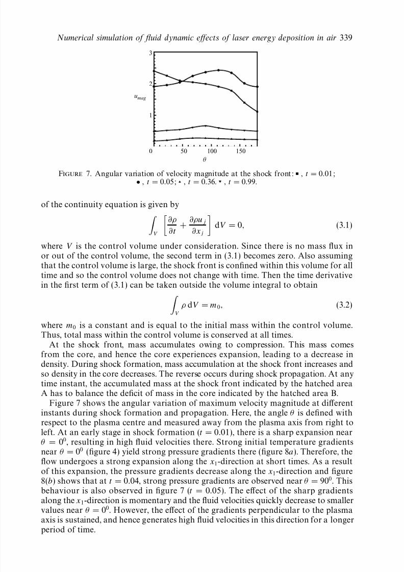
Figure 7. Angular variation of velocity magnitude at the shock front: , t = 0 .01;• , t = 0 .05; , t = 0 .36. , t = 0 .99.

of the continuity equation is given by

V

∂ρ∂t

+ ∂ρu j

∂x j dV = 0 , (3.1)

where V is the control volume under consideration. Since there is no mass ux inor out of the control volume, the second term in (3.1) becomes zero. Also assumingthat the control volume is large, the shock front is conned within this volume for alltime and so the control volume does not change with time. Then the time derivativein the rst term of (3.1) can be taken outside the volume integral to obtain

V ρ dV = m0, (3.2)

where m0 is a constant and is equal to the initial mass within the control volume.Thus, total mass within the control volume is conserved at all times.

At the shock front, mass accumulates owing to compression. This mass comesfrom the core, and hence the core experiences expansion, leading to a decrease indensity. During shock formation, mass accumulation at the shock front increases andso density in the core decreases. The reverse occurs during shock propagation. At anytime instant, the accumulated mass at the shock front indicated by the hatched areaA has to balance the decit of mass in the core indicated by the hatched area B.

Figure 7 shows the angular variation of maximum velocity magnitude at differentinstants during shock formation and propagation. Here, the angle θ is dened withrespect to the plasma centre and measured away from the plasma axis from right toleft. At an early stage in shock formation ( t = 0 .01), there is a sharp expansion nearθ = 0 0, resulting in high uid velocities there. Strong initial temperature gradientsnear θ = 0 0 (gure 4) yield strong pressure gradients there (gure 8 a ). Therefore, theow undergoes a strong expansion along the x1-direction at short times. As a resultof this expansion, the pressure gradients decrease along the x1-direction and gure8(b) shows that at t = 0 .04, strong pressure gradients are observed near θ = 90 0. Thisbehaviour is also observed in gure 7 ( t = 0 .05). The effect of the sharp gradients

along the x1-direction is momentary and the uid velocities quickly decrease to smallervalues near θ = 0 0. However, the effect of the gradients perpendicular to the plasmaaxis is sustained, and hence generates high uid velocities in this direction for a longerperiod of time.




(a) (b)

Figure 8. Contours of pressure at ( a ) t = 0 and ( b) t = 0 .04 showing development of astrong shock wave in the direction normal to the plasma axis.

(a) (b)

Figure 9. Contours of pressure at ( a ) t = 0.36 and ( b) t = 0.99 shows that the shock wavebecomes spherical in time as it propagates into the background.

umag

r 0.4 0.8 1.2

0

1

2

3 (a) (b)

r 1.0 1.5 2.0 2.5

0

0.2

0.4

Figure 10. (a ) Radial proles for velocity magnitude plotted along different angles from thecentre of the plasma at t = 0 .04 show distinct angular asymmetry. ( b) Similar proles forvelocity magnitude at t = 0 .99. , θ = 90 ◦ ; , θ = 180 ◦ .

Figure 9 shows that as the shock wave propagates into the background, it becomesspherical in shape. Also its strength becomes uniform over θ . This is also observedin the angular variation of velocity magnitude shown in gure 7. Figure 10 shows

radial proles of velocity magnitude plotted along θ = 90◦

and θ = 180◦

at t = 0 .05and 0 .99. The sharper gradients perpendicular to the plasma axis at t = 0 .04 resultin stronger acceleration of the uid elements in this direction, thus making the shockwave more spherical in time.




t = 0.18

t = 0.48

t = 0.99 t = 0.44 t = 1.62

t = 0.72 t = 0.81

t = 0.30 t = 0.36

Figure 11. Plots of velocity streamlines showing evolution of the ow eld in time.

3.1.2. Roll-up of the plasma coreAs the shock wave propagates outwards, the temperatures in the plasma core decay

in an interesting manner. The initial axial temperature prole has a single peak (gure4a ). In time, this peak advects to the left and yields a single centre of expansion,as observed at t = 0 .18 in gure 11. However, the temperatures in the plasma coredecay such that the axial temperature prole splits to form two independent centresof expansion ( t = 0 .30). This behaviour is also observed in experiments (e.g. Glumacet al . 2005a, b). The second expansion point is initially weaker than the rst, but as thecore temperatures continue to decay, the two expansion points become comparable instrength ( t = 0 .36). Since the temperatures decay faster near the rst expansion point,the second expansion point soon becomes much stronger than the rst. Fluid thenaccelerates from right to left, towards the rst expansion point ( t = 0 .48). Interactionof the uid rushing in from the right with that issuing from the rst expansionpoint results in the ow turning normal to the plasma axis. The ow evolves to formcomplex vortical structures (gure 11) which nally yield the toroidal vortex ringobserved in experiments (Adelgren et al. 2003; Glumac et al. 2005a, b).

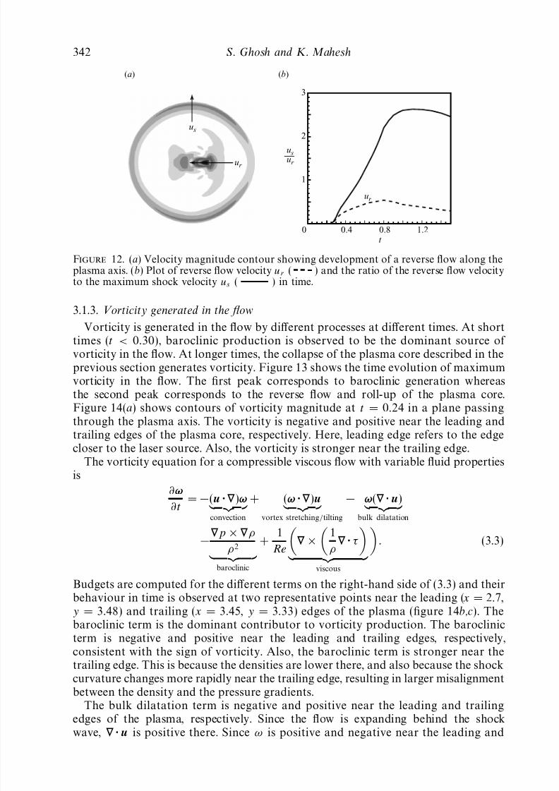
Note that when the plasma is initially expanding, the ow along the plasma axis isfrom left to right. However, in time, the direction of ow along the axis is reversed.The reverse ow builds up in strength and signicantly exceeds the velocity at theshock front (gure 12).




(a) (b)

ur ur

u s

u s

t 0 0.4 0.8 1.2

1

2

3

ur

Figure 12. (a) Velocity magnitude contour showing development of a reverse ow along theplasma axis. ( b) Plot of reverse ow velocity u r ( ) and the ratio of the reverse ow velocityto the maximum shock velocity us ( ) in time.

3.1.3. Vorticity generated in the owVorticity is generated in the ow by different processes at different times. At short

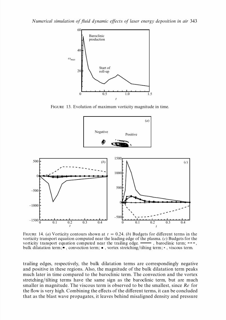
times ( t < 0.30), baroclinic production is observed to be the dominant source of vorticity in the ow. At longer times, the collapse of the plasma core described in theprevious section generates vorticity. Figure 13 shows the time evolution of maximumvorticity in the ow. The rst peak corresponds to baroclinic generation whereasthe second peak corresponds to the reverse ow and roll-up of the plasma core.Figure 14( a) shows contours of vorticity magnitude at t = 0 .24 in a plane passingthrough the plasma axis. The vorticity is negative and positive near the leading andtrailing edges of the plasma core, respectively. Here, leading edge refers to the edgecloser to the laser source. Also, the vorticity is stronger near the trailing edge.

The vorticity equation for a compressible viscous ow with variable uid propertiesis

∂ ω

∂t = − (u · ∇ )ω

convection

+ ( ω · ∇ )u

vortex stretching / tilting

− ω (∇ · u )

bulk dilatation

−∇ p × ∇ ρ

ρ2

baroclinic

+ 1

Re

∇ ×1

ρ

∇ · τ

viscous

. (3.3)

Budgets are computed for the different terms on the right-hand side of (3.3) and theirbehaviour in time is observed at two representative points near the leading ( x = 2 .7,y = 3 .48) and trailing ( x = 3 .45, y = 3 .33) edges of the plasma (gure 14 b,c). Thebaroclinic term is the dominant contributor to vorticity production. The baroclinicterm is negative and positive near the leading and trailing edges, respectively,consistent with the sign of vorticity. Also, the baroclinic term is stronger near thetrailing edge. This is because the densities are lower there, and also because the shockcurvature changes more rapidly near the trailing edge, resulting in larger misalignment

between the density and the pressure gradients.The bulk dilatation term is negative and positive near the leading and trailingedges of the plasma, respectively. Since the ow is expanding behind the shockwave, ∇ · u is positive there. Since ω is positive and negative near the leading and




ω max

t 0 0.5 1.0 1.5

20

40

60

Baroclinic production

Start of roll-up

Figure 13. Evolution of maximum vorticity magnitude in time.

Positive Negative

(a)

(b) (c)

t 0 0.1 0.2 0.3 0.4

–500

–1000

–1500

0

500

t 0 0.1 0.2 0.3 0.4

–500

0

500

1000

1500

Figure 14. (a) Vorticity contours shown at t = 0 .24. (b) Budgets for different terms in thevorticity transport equation computed near the leading edge of the plasma. ( c) Budgets for thevorticity transport equation computed near the trailing edge. , baroclinic term; ,bulk dilatation term; , convection term; • , vortex stretching/tilting term; , viscous term.

trailing edges, respectively, the bulk dilatation terms are correspondingly negativeand positive in these regions. Also, the magnitude of the bulk dilatation term peaksmuch later in time compared to the baroclinic term. The convection and the vortex

stretching/tilting terms have the same sign as the baroclinic term, but are muchsmaller in magnitude. The viscous term is observed to be the smallest, since Re forthe ow is very high. Combining the effects of the different terms, it can be concludedthat as the blast wave propagates, it leaves behind misaligned density and pressure




(a ) (b)

(c)

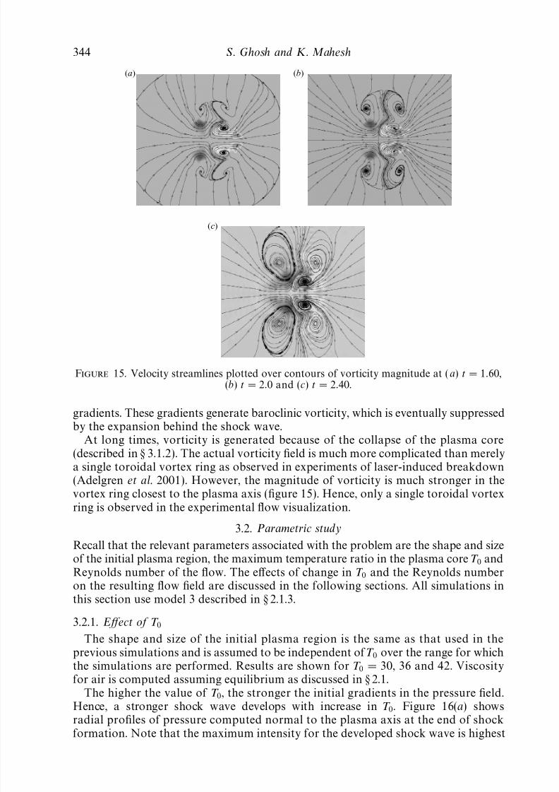
Figure 15. Velocity streamlines plotted over contours of vorticity magnitude at ( a) t = 1 .60,(b) t = 2 .0 and ( c) t = 2 .40.

gradients. These gradients generate baroclinic vorticity, which is eventually suppressedby the expansion behind the shock wave.At long times, vorticity is generated because of the collapse of the plasma core

(described in §3.1.2). The actual vorticity eld is much more complicated than merelya single toroidal vortex ring as observed in experiments of laser-induced breakdown(Adelgren et al. 2001). However, the magnitude of vorticity is much stronger in thevortex ring closest to the plasma axis (gure 15). Hence, only a single toroidal vortexring is observed in the experimental ow visualization.

3.2. Parametric studyRecall that the relevant parameters associated with the problem are the shape and sizeof the initial plasma region, the maximum temperature ratio in the plasma core T 0 andReynolds number of the ow. The effects of change in T 0 and the Reynolds numberon the resulting ow eld are discussed in the following sections. All simulations inthis section use model 3 described in §2.1.3.

3.2.1. Effect of T 0The shape and size of the initial plasma region is the same as that used in the

previous simulations and is assumed to be independent of T 0 over the range for whichthe simulations are performed. Results are shown for T 0 = 30, 36 and 42. Viscosityfor air is computed assuming equilibrium as discussed in §2.1.

The higher the value of T 0, the stronger the initial gradients in the pressure eld.Hence, a stronger shock wave develops with increase in T 0. Figure 16( a) showsradial proles of pressure computed normal to the plasma axis at the end of shockformation. Note that the maximum intensity for the developed shock wave is highest




p

r 3.2 3.6 4.0

0

4

8

12

t = 0.3

0.4

0.5

(a)

(c)

(b)

r 3.5 4.0 4.5 5.0

0.5

1.0

1.5

p

0 50 100θ

150

4

8

12

Figure 16. (a) Radial pressure proles ( θ = 90 ◦ ) for T 0 = 30 ( ), T 0 = 36 ( ) andT 0 = 42 ( ) at the end of shock formation for each case. ( b) Radial pressure proles(θ = 90 ◦ ) for T 0 = 30 ( ), T 0 = 36 ( ) and T 0 = 42 ( ) at t = 0 .45. (c) Angularvariation of pressure at the shock front at the instant when it is maximum. , T 0 = 30; ,T 0 = 36; • , T 0 = 42.

for T 0 = 42. Also, the shock formation time is smallest for T 0 = 42 and largest forT 0 = 30. The process of conversion of internal energy into kinetic energy is also fasterwith increase in energy deposited.

Since the pressure gradients are strongest for T 0 = 42, higher shock velocities aredeveloped. Thus, if proles are compared at the same time instant, the shock wavefor T 0 = 42 will have propagated farthest (gure 16 b). Proles of pressure computednormal to the plasma axis at t = 0 .45 are shown for different T 0. The shock radius islargest for T 0 = 42 and smallest for T 0 = 30. Figure 16( c) shows the angular variationof pressure at the shock front at the end of the shock-formation process. The angle θ is dened as described in §3.1.1. Note that the shock strength increases with increasein T 0, but the angular spread of the shock strength does not change much.

Figure 17( a) shows the maximum reverse ow magnitude ur for different T 0. Forhigher T 0, stronger reverse ows are obtained. However, the overall trend remainsthe same for different T 0. Recall that this reverse ow was found to be responsiblefor generating vorticity in the ow at long times. Figure 17( b) shows evolution of

the maximum vorticity magnitude in time for different T 0. The stronger the reverseow developed, the higher the magnitude of vorticity generated. Also the baroclinicvorticity generated at short times is observed to be stronger for higher T 0. This isbecause, as discussed in §3.1.3, the baroclinic vorticity generated depends directly




ur

t 0.2 0.4 0.6 0.8 1.00

0.2

0.4

0.6

0.8(a) (b)

ω max

t 0 0.5 1.0 1.5

40

80

120

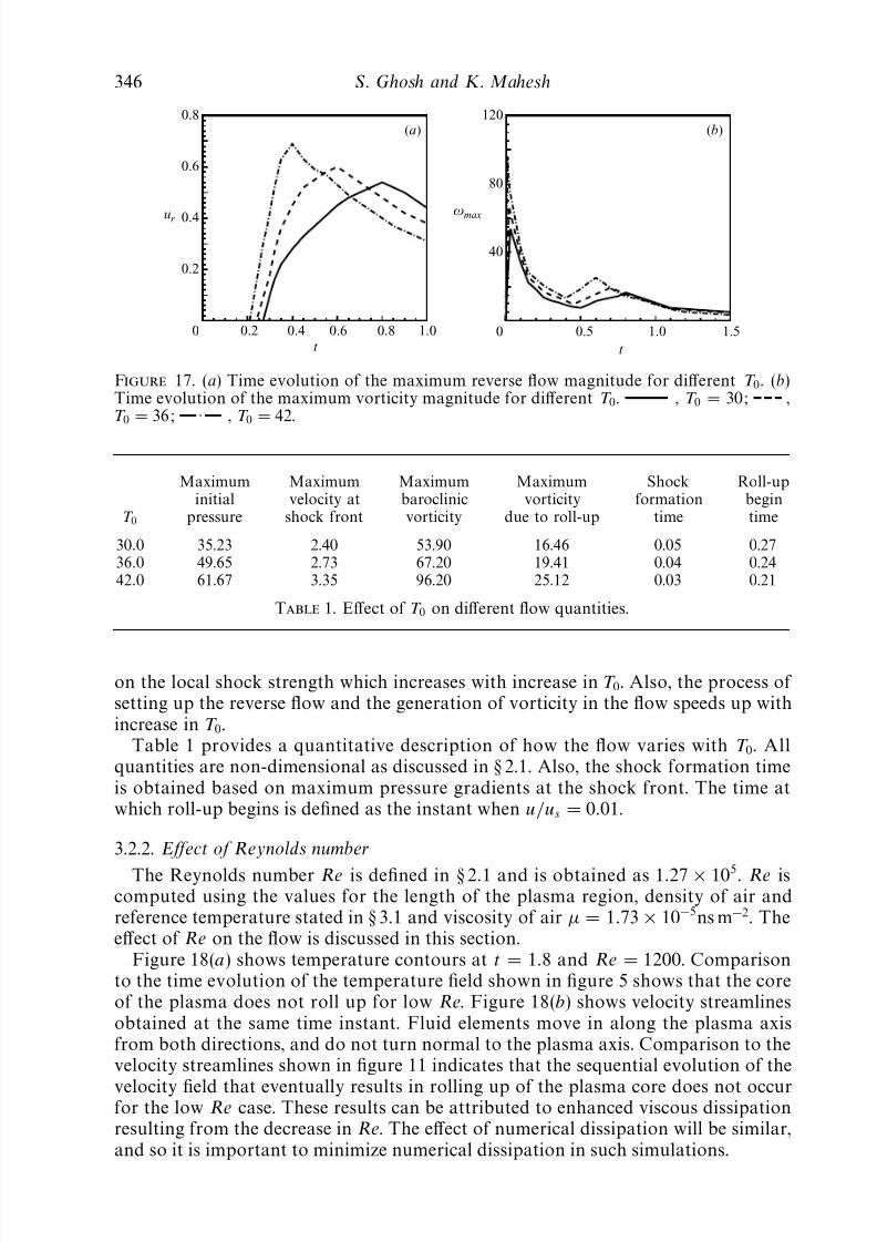
Figure 17. (a) Time evolution of the maximum reverse ow magnitude for different T 0. (b)Time evolution of the maximum vorticity magnitude for different T 0. , T 0 = 30; ,T 0 = 36; , T 0 = 42.

Maximum Maximum Maximum Maximum Shock Roll-upinitial velocity at baroclinic vorticity formation begin

T 0 pressure shock front vorticity due to roll-up time time

30.0 35.23 2.40 53.90 16.46 0.05 0.2736.0 49.65 2.73 67.20 19.41 0.04 0.2442.0 61.67 3.35 96.20 25.12 0.03 0.21

Table 1. Effect of T 0 on different ow quantities.

on the local shock strength which increases with increase in T 0. Also, the process of setting up the reverse ow and the generation of vorticity in the ow speeds up withincrease in T 0.

Table 1 provides a quantitative description of how the ow varies with T 0. Allquantities are non-dimensional as discussed in §2.1. Also, the shock formation timeis obtained based on maximum pressure gradients at the shock front. The time atwhich roll-up begins is dened as the instant when u/u s = 0 .01.

3.2.2. Effect of Reynolds number

The Reynolds number Re is dened in §2.1 and is obtained as 1 .27 × 105. Re iscomputed using the values for the length of the plasma region, density of air andreference temperature stated in §3.1 and viscosity of air µ = 1 .73 × 10− 5ns m − 2. Theeffect of Re on the ow is discussed in this section.

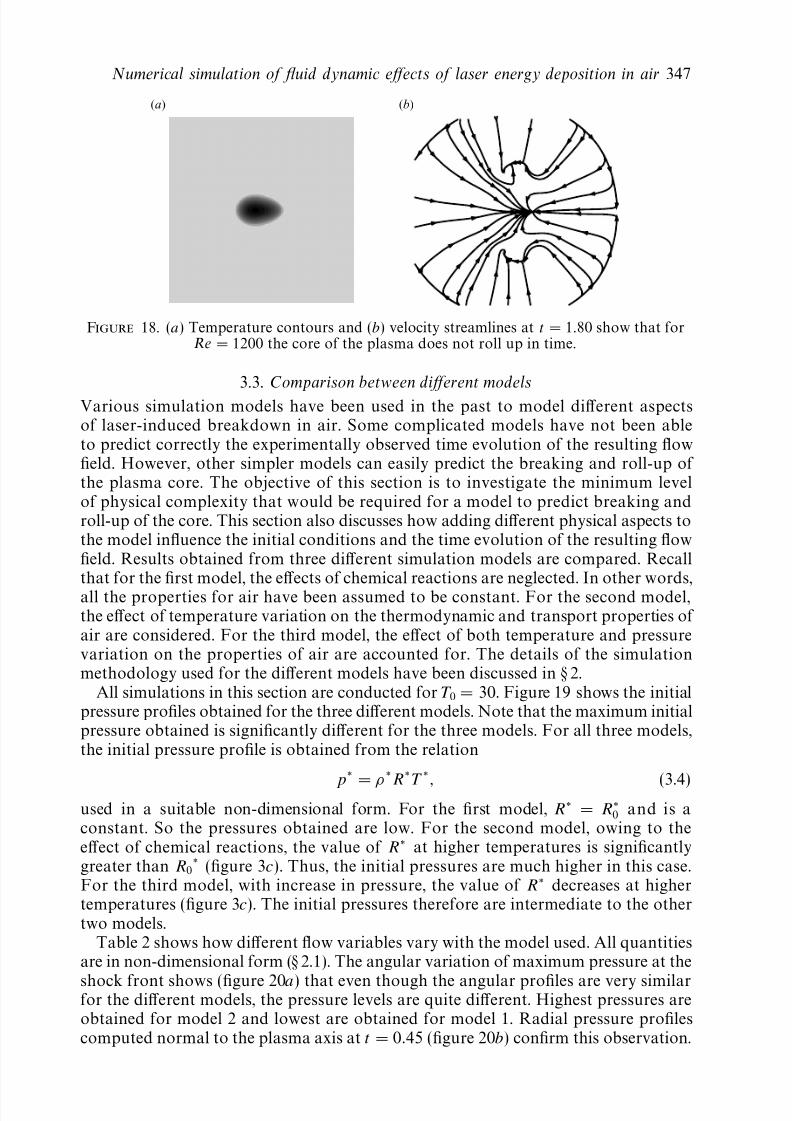
Figure 18( a ) shows temperature contours at t = 1 .8 and Re = 1200. Comparisonto the time evolution of the temperature eld shown in gure 5 shows that the coreof the plasma does not roll up for low Re. Figure 18( b) shows velocity streamlinesobtained at the same time instant. Fluid elements move in along the plasma axisfrom both directions, and do not turn normal to the plasma axis. Comparison to thevelocity streamlines shown in gure 11 indicates that the sequential evolution of the

velocity eld that eventually results in rolling up of the plasma core does not occurfor the low Re case. These results can be attributed to enhanced viscous dissipationresulting from the decrease in Re. The effect of numerical dissipation will be similar,and so it is important to minimize numerical dissipation in such simulations.




(a ) (b)

Figure 18. (a ) Temperature contours and ( b) velocity streamlines at t = 1 .80 show that forRe = 1200 the core of the plasma does not roll up in time.

3.3. Comparison between different modelsVarious simulation models have been used in the past to model different aspectsof laser-induced breakdown in air. Some complicated models have not been ableto predict correctly the experimentally observed time evolution of the resulting oweld. However, other simpler models can easily predict the breaking and roll-up of the plasma core. The objective of this section is to investigate the minimum levelof physical complexity that would be required for a model to predict breaking androll-up of the core. This section also discusses how adding different physical aspects tothe model inuence the initial conditions and the time evolution of the resulting oweld. Results obtained from three different simulation models are compared. Recallthat for the rst model, the effects of chemical reactions are neglected. In other words,all the properties for air have been assumed to be constant. For the second model,the effect of temperature variation on the thermodynamic and transport properties of air are considered. For the third model, the effect of both temperature and pressurevariation on the properties of air are accounted for. The details of the simulationmethodology used for the different models have been discussed in §2.

All simulations in this section are conducted for T 0 = 30. Figure 19 shows the initialpressure proles obtained for the three different models. Note that the maximum initialpressure obtained is signicantly different for the three models. For all three models,the initial pressure prole is obtained from the relation

p∗

= ρ∗

R∗

T ∗

, (3.4)used in a suitable non-dimensional form. For the rst model, R∗ = R∗0 and is aconstant. So the pressures obtained are low. For the second model, owing to theeffect of chemical reactions, the value of R∗ at higher temperatures is signicantlygreater than R0

∗ (gure 3c). Thus, the initial pressures are much higher in this case.For the third model, with increase in pressure, the value of R∗ decreases at highertemperatures (gure 3 c). The initial pressures therefore are intermediate to the othertwo models.

Table 2 shows how different ow variables vary with the model used. All quantitiesare in non-dimensional form ( §2.1). The angular variation of maximum pressure at the

shock front shows (gure 20 a ) that even though the angular proles are very similarfor the different models, the pressure levels are quite different. Highest pressures areobtained for model 2 and lowest are obtained for model 1. Radial pressure prolescomputed normal to the plasma axis at t = 0 .45 (gure 20b) conrm this observation.




(a) (b)

(c)

2 4 6 8 10 12 14 16 18 20

2 6 10 14 18 22 26 30 34

2 6 10 14 18 22 26 30 34 38 42

Figure 19. Initial pressure contours obtained for three different models, ( a ) model 1, (b)model 2 and ( c) model 3.

Maximum Maximum Maximum Maximum Shock Roll-upModel initial velocity at baroclinic vorticity formation begin

(T 0 = 30) pressure shock front vorticity due to roll-up time time

1 21.07 1.69 28.45 12.06 0.06 0.302 42.89 2.87 63.78 18.81 0.04 0.253 35.23 2.40 53.90 16.46 0.05 0.27

Table 2. Variation of different ow quantities with the simulation model used.

The evolution of the ow eld is qualitatively similar for all three models (gure 21).However, the extent to which the ow has evolved at any given time is different. Atany instant, all three models yield different stages of the characteristic ow evolutionsequence shown in gure 11. Since the pressure gradients are weakest for the rstmodel, the ow eld evolves slowly when compared to the other cases. Hence, only asingle expansion centre is observed. For the second model, the ow eld evolves fasterthan the other cases. Hence, two distinct expansion centres of comparable strengthare observed. The ow eld obtained from model 3 evolves to a stage intermediatebetween that obtained from models 1 and 2. For all three models, the ow eldeventually rolls up. Even an ideal-gas representation is sufficient to predict the roll-upof the plasma core.

4. SummaryThis paper uses numerical simulation to study the effect of laser energy deposition

on quiescent air. Local thermodynamic equilibrium conditions are assumed to apply.

The simulations solve the compressible Navier–Stokes equations using Fourier spectralmethods. A predictor–corrector-based shock-capturing scheme is incorporated toaccount for the strong shock waves. Three different models are used to obtain thethermodynamic and transport properties for air. For model 1, the effects of the




p

0 50 100θ

150

2

4

6

8(a) (b)

r 3.5 4.0 4.5

0

0.4

0.8

1.2

1.6

Figure 20. (a ) Angular variation of pressure at the shock front at the instant when it ismaximum. • , model 1; , model 2; , model 3. ( b) Radial pressure proles ( θ = 90 0) formodel 1 ( ), model 2 ( ) and model 3 ( ) at t = 0 .45 .

(a)

(c)

(b)

Figure 21. Comparison of velocity streamlines from different models at t = 0 .3, (a ) model1, (b) model 2 and ( c) model 3.

chemical reactions are neglected and uid properties are assumed to be constant.For model 2, the properties are assumed to vary with temperature alone. Model 3accounts for both temperature and pressure variation of the properties of air. Foreach model, the corrector step of the shock-capturing scheme is suitably modied.Also, a logarithmic formulation for the continuity equation is developed to handlelow densities at the core of the plasma.

The evolution of the ow eld is classied into formation of a shock wave, itspropagation into the background and subsequent collapse of the plasma core. Eachphase is studied in detail. Formation and propagation of the shock wave is explainedbased on conservation of mass behind the shock front. The ow is driven by the




gradients in the pressure eld. The shock wave is stronger normal to the plasmaaxis and the angular variation of the shock strength is discussed. As the shock wavepropagates into the background, its asymmetry decreases and it becomes spherical intime.

Behind the shock wave, a strong reverse ow is observed along the plasma axis. Thisreverse ow initially increases in strength to a maximum and then gradually decays.The reverse ow generates a complicated vortical eld with a prominent toroidal ringvortex. The process is explained.

Vorticity is generated in the ow through different mechanisms. At short times,vorticity is generated by baroclinic means. At longer times, vorticity is generated as aresult of the reverse ow in the plasma core.

The effects of deposited laser energy and Reynolds number are discussed. Jumps atthe shock front scale with the initial pressure gradients and hence with the amountof energy deposited in the ow. However, the propagation of the shock wave andformation of the reverse ow are qualitatively similar for different amount of energy

deposited. The plasma core does not roll-up at very low Re.Results obtained from simulations conducted using three different models for airare compared. The initial pressure elds are found to be signicantly different forthe three models. Again, the results are found to scale with the initial gradients inthe pressure eld. However, the ow eld is found to evolve in a qualitatively similarmanner for all three models.

This work is supported by the United States Air Force Office of ScienticResearch under grant FA-9550-04-1-0064. Computing resources were provided bythe Minnesota Supercomputing Institute, the San Diego Supercomputing Center, andthe National Center for Supercomputing Applications. We are thankful to Dr NomaPark for useful discussions.

AppendixThe Jacobian matrix for the corrector step of the shock-capturing scheme is

reconstructed based on the assumption that the thermodynamic properties arefunctions of pressure and temperature. The Jacobian matrix for the x-direction isobtained as

J x =

0

− u 2 + 1θ 1

(RT − G 1 − A (e − ek))

− vu− wu

− (A (e − ek) + e0 + G 1 + G 1G 2 − RT G 2)

1 0 0 0

2 − Aθ

1

u −Aθ

1

v −Aθ

1

w A

θ 1v u 0 0

w 0 u 0(e0 + RT − A u 2) − A uv ) − A uw ) (1 + A )u




where A and A are given by,

A = A (1 + G 2), A = R + T ∂R∂T

1θ 2

, (A1)

G 1 and G 2 are given by

G 1 = Ap

θ 1

∂e∂p

, G 2 = ρT

θ 1

∂R∂p

, (A2)

and θ 1 and θ 2 are given by

θ 1 = 1 − pR

∂R∂p

, θ 2 = ∂e∂T

+ ∂e∂p

pT

+ pR

∂R∂T

1 − pR

∂R∂p

. (A3)

This form of the Jacobian matrix is used for simulations using model 3. The right and

left eigen vector matrices R and L are computed numerically. Note that the Jacobianmatrix is easily reducible to models 2 and 1. For model 2, the gradients of e and Rwith respect to pressure are neglected. Hence, G 1 and G 2 become

G 1 = G 2 = 0 , (A4)θ 1 and θ 2 simplify to give

θ 1 = 1 , θ 2 = dedT

, (A5)

and

A = A = R + T ∂R∂T

dT de

. (A6)

The Jacobian matrix is given by

J x =

0 1 0 0 0(− u 2 + RT − A (e − ek)) (2 − A ) ∗ u − Av − Aw A

− vu v u 0 0− wu w 0 u 0

− (e0 + A (e − ek))u (e0 + RT − Au 2) − Auv − Auw (1 + A )u.

.

Dene a set of variables e1 and e2 such that

e1 =

c12

A(A + 1) (A7)

ande2 = e − e1. (A8)

Also dene ek∗ such that

ek∗= ek − e2. (A9)

Then the right and left eigen vector matrices R and L for the x-direction are thenobtained as

R x =

1 1 1 0 0u − c1 u u + c1 0 0

v v v − 1 0w w w 0 1

(h 0 − c1u ) ek∗ (h 0 + c1u ) − v w

,




and

R X =

Ae k∗+ c1u2c1

2 −Au + c1

2c12 −

Av2c1

2 − Aw2c1

2A

2c12

c12 − Ae k

∗

c12

Au

c12

Av

c12

Aw

c12 −

A

c12

Ae k∗− c1u2c1

2 −Au − c1

2c12 −

Av2c1

2 − Aw2c1

2A

2c12

v 0 − 1 0 0− w 0 0 1 0

where h0 is the total enthalpy given by

h 0 = h + ek . (A10)

Similarly, eigen vectors RY , RZ , L Y and L Z can be computed along the y- andz-directions, respectively.

The Jacobian matrix can be further be simplied for model 1. Then A furthersimplies to

A = ( γ − 1), (A11)and the Jacobian matrix is given by

J x =

0(− u 2 + RT − (γ − 1)(e − ek))

− vu− wu

− (e0 + ( γ − 1)(e − ek))u

1 0 0 0(3 − γ ) ∗ u − (γ − 1)v − (γ − 1)w (γ − 1)

v u 0 0w 0 u 0

(e0 + RT − (γ − 1)u 2) − (γ − 1)uv − (γ − 1)uw γ u

.

Thus, the Jacobian matrix then reduces to its standard low-temperature form (Rohde2001). Similar Jacobian matrices can be constructed for the y- and z-directions. Theeigen vector matrices R and L can be similarly simplied.

REFERENCES

Adelgren, R., Boguszko, M. & Elliott, G. 2001 Experimental summary report – shockpropagation measurements for Nd:YAG laser induced breakdown in quiescent air.Department of Mechanical and Aerospace Engineering, Rutgers University.

Adelgren, R. G., Yan, H., Elliott, G. S., Knight, D., Beutner, T. J., Zheltovodov, A., Ivanov,M. & Khotyanovsky, D. 2003 Localized ow control by laser energy deposition applied toEdney IV shock impingement and intersecting shocks. AIAA Paper 2003–31.

Blaisdell, G. A., Mansour, N. N. & Reynolds, W. C. 1991 Numerical simulations of compressiblehomogeneous turbulence. Report TF-50, Thermosciences Division, Department of MechanicalEngineering, Stanford University.

Brode, H. L. 1955 Numerical solution of blast waves. J. Appl. Phys. 26 , 766–775.



Numerical simulation of uid dynamic effects of laser energy deposition in air 353Damon, E. & Tomlinson, R. 1963 Observation of ionization of gases by a ruby laser. Appl. Optics 2 ,

546–547.Dors, I. G. & Parigger, C. G. 2003 Computational uid-dynamic model of laser induced breakdown

in air. Appl. Optics 42 , 5978–5985.Dors, I., Parigger, C. & Lewis, J. 2000 Fluid dynamic effects following laser-induced optical

breakdown. AIAA Paper 2000–0717.Glumac, N., Elliott, G. & Boguszko, M. 2005a Temporal and spatial evolution of thermal

structure of laser spark in air. AIAA J. 43 , 1984–1994.Glumac, N., Elliott, G. & Boguszko, M. 2005b Temporal and spatial evolution of the thermal

structure of a laser spark in air. AIAA Paper 2005–0204.Harten, A. 1978 The articial compression method for computation of shocks and contact

discontinuities. Maths Comput. 32 , 363.Hayes, W. D. 1957 The vorticity jump across a gasdynamic discontinuity. J. Fluid Mech. 2 , 595–600.Jiang, Z., Takayama, K., Moosad, K. P. B., Onodera, O. & Sun, M. 1998 Numerical and

experimental study of a micro-blast wave generated by pulsed laser beam focusing. Shockwaves 8 , 337–349.

Kandala, R. 2005 Numerical simulations of laser energy deposition for supersonic ow control.

PhD thesis, Department of Aerospace Engineering and Mechanics, University of Minnesota.Kandala, R. & Candler, G. 2003 Numerical studies of laser-induced energy deposition forsupersonic ow control. AIAA Paper 2003–1052.

Kandala, R., Candler, G., Glumac, N. & Elliott, G. 2005 Simulation of laser-induced plasmaexperiments for supersonic ow control. AIAA Paper 2005–0205.

Keefer, D. 1989 Laser-sustained plasmas. In Laser-Induced Plasmas and Applications (ed. L. J.Radziemski & D. A. Cremers) Marcel Dekker.

Knight, D., Kuchinskiy, V., Kuranov, A. & Sheikin, E. 2003 Survey of aerodynamic ow controlat high speed by energy deposition. AIAA Paper 2003–0525.

Lee, J. H. 2005 Electron-impact vibrational relaxation in high temperature nitrogen. AIAA Paper1992–0807.

Lewis, J., Parigger, C., Hornkohl, J. & Guan, G. 1999 Laser-induced optical breakdown plasma

spectra and analysis by use of the program NEQAIR. AIAA Paper 99–0723.McBride, B. J. & Gordon, S. 1961 Thermodynamic functions of several triatomic molecules in theideal gas state. J. Chem. Phys 35 , 2198–2206.

McBride, B. J. & Gordon, S. 1967 FORTRAN IV program for calculation of thermodynamicdata. NASA SP 3001.

McBride, B. J. & Gordon, S. 1976 Computer program for computation of complex chemicalequilibrium compositions, rocket performance, incident and reected shocks, and Chapman–Jouguet detonations. NASA SP 273.

McBride, B. J. & Gordon, S. 1992 Computer program for calculating and tting thermodynamicfunctions. NASA RP 1271.

McBride, B. J., Heimel, S., Ehlers, J. & Gordon, S. 1963 Thermodynamic properties to 6000 Kfor 210 substances involving the rst 18 elements. NASA SP 3001.

Maker, P., Terhune, R. & Savage, C. 1963 Proc. Third Intl. Quantum Mechanics Conf. Paris .Meyerand, R. & Haught, A. 1963 Gas breakdown at optical frequencies. Phys. Rev. Lett. 11 , 401–

403.Molina-Morales, P., Toyoda, K., Komurasaki, K. & Arakawa, Y. 2001 CFD simulation of a

2-kW class laser thruster. AIAA Paper 2001–0650.Morgan, C. 1975 Laser-induced breakdown of gases. Rep. Prog. Phys. 38 , 621–665.Phuoc, T. X. 2000 Laser spark ignition: experimental determination of laser-induced breakdown

thresholds of combustion gases. Optics Commun. 175 , 419–423.Phuoc, T. X. 2005 An experimental and numerical study of laser-induced spark in air. Optics Lasers

Engng 43 , 113–129.Raizer, Y. P 1966 Breakdown and heating of gases under the inuence of a laser beam. Sov. Phys.

USPEKHI 8 , 650–673.Riggins, D. W., Nelson, H. F. & Johnson, E. 1999 Blunt-body wave drag reduction using focused

energy deposition. AIAA J. 37 , 460–467.Rohde, A. 2001 Eigen values and eigen vectors of the Euler equations in general geometries. AIAA

Paper 2001–2609.




Root, R. G. 1989 Modeling of Post-Breakdown Phenomenon in Laser-Induced Plasma and Applications , vol. 2, pp. 69–103. Marcel Dekker.

Shneider, M. N., Macheret, S. O., Zaidi, S. H., Girgis, I. G., Raizer, Yu. P. & Miles, R. B. 2003Steady and unsteady supersonic ow control with energy addition. AIAA Paper 2003–3862.

Steiner, H., Gretler, W. & Hirschler, T. 1998 Numerical solution for spherical laser-driven shockwaves. Shock Waves 8 , 337–349.

Wang, T. S., Chen, Y. S., Liu, J., Myrabo, L. N. & Mead, F. B. 2001 Advanced performancemodeling of experimental laser lightcrafts. AIAA Paper 2001–0648.

Yan, H., Adelgren, M., Bouszko, M., Elliott, G. & Knight, D. 2003 Laser energy deposition inquiescent air AIAA Paper 2003–1051.

Yee, H. C., Sandham, N. D. & Djomehri, M. J. 1999 Low-dissipative high-order shock-capturingmethods using characteristic-based lter. J. Comput. Phys. 150 , 199–238.

shankar jfm thermal

Documents