session 17, introduction to economic capital 17, introduction to economic capital moderator: adam...

Session 17, Introduction to Economic Capital

Moderator: Adam Koursaris

Presenters: Prabhdeep Singh, FSA, CERA, MAAA

Introduction to Economic Capital

Adam [email protected]

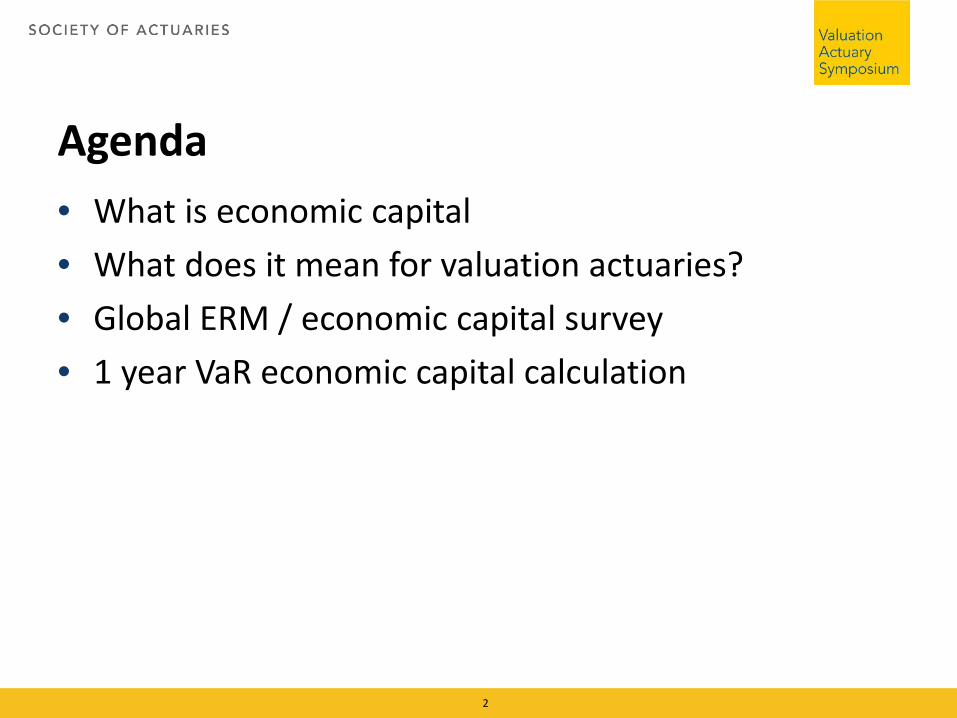
Agenda• What is economic capital• What does it mean for valuation actuaries?• Global ERM / economic capital survey• 1 year VaR economic capital calculation

2

What is Economic Capital• BIS 2009: “Economic capital can be defined as the methods or practices that allow banks to

consistently assess risk and attribute capital to cover the economic effects of risk-taking activities.”

• SOA / Towers Perrin 2008: “The term “economic capital” is typically used to refer to a measure of required capital under an economic accounting convention ⎯ where assets and liabilities are determined using economic principles.”

• Wikipedia: “economic capital is the amount of risk capital, assessed on a realistic basis, which a firm requires to cover the risks that it is running or collecting as a going concern, such as market risk, credit risk, legal risk, and operational risk. It is the amount of money which is needed to secure survival in a worst-case scenario.

• Investopedia: Economic capital (EC) is the amount of risk capital that a bank estimates in order to remain solvent at a given confidence level and time horizon.

• A. J. McNeil 2005: Economic capital offers a firm-wide language for discussing and pricing risk that is related directly to the principal concerns of management and other stakeholders, namely institutional solvency and profitability. […] Economic capital is so called because it measures risk in terms of economic realities, rather than potentially misleading regulatory or accounting rules.

3

Economic Reality?• A failure to pay cashflows is a certain way to experience

economic reality

• Commentators often interpret economic balance sheet to mean market-consistent, including the cost of options and guarantees

• A legal definition: “Economic realities test refers to a method that determines the nature of a business transaction by examining the totality of the commercial circumstances.”

4

Time horizon• There are two main schools of thought in EC calculation:

– 1 year– Run-off

• Both have unique features

5

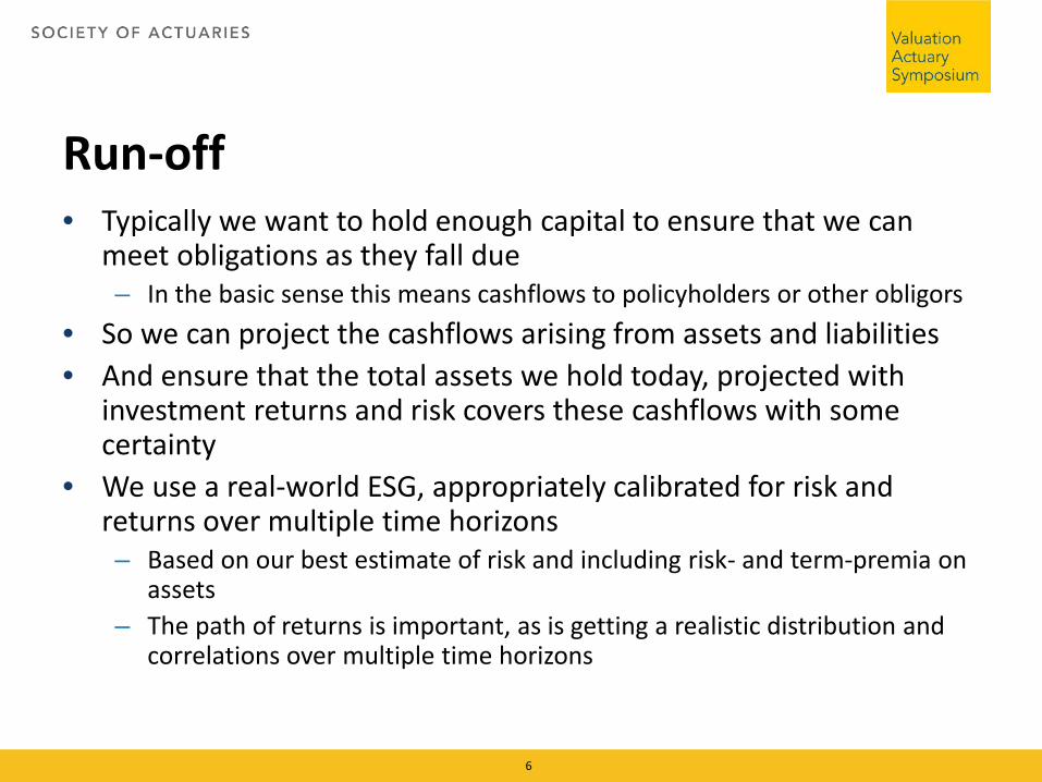
Run-off• Typically we want to hold enough capital to ensure that we can

meet obligations as they fall due– In the basic sense this means cashflows to policyholders or other obligors

• So we can project the cashflows arising from assets and liabilities • And ensure that the total assets we hold today, projected with

investment returns and risk covers these cashflows with some certainty

• We use a real-world ESG, appropriately calibrated for risk and returns over multiple time horizons– Based on our best estimate of risk and including risk- and term-premia on

assets– The path of returns is important, as is getting a realistic distribution and

correlations over multiple time horizons

6

Run-off A run-off approach recognizes the long-term nature of life insurance

operations, liabilities and investment It is often argued that a lot of day-to-day market volatility is not important

over the long term – particularly for things like credit spreads Systemically, a run-off approach usually promotes stability in capital levels

and avoids pro-cyclicality

Run-off approaches typically ignore intermediate forward looking assessments– It will not be the failure to pay cashflows that results in losses for policyholders

– regulators will step in long before then (we hope)– What are the assessment conditions now? And what will they be in 20 years

time? A run-off approach can become unhinged from market conditions

– You may have an EC deficiency but be unable to improve the capital position through risk reduction strategies like hedging, reinsurance, securitizations or capital markets transactions because the market cost of these transactions is more onerous than the economic capital held

7

1 Year• Typically we measure the market-consistent embedded value of net

assets in 1 year’s time• And ensure that the total assets we hold today, projected with

investment returns and risk covers this value with a given certainty• We use a 1 year real-world ESG to measure risk

– Based on our best estimate of risk and returns, including risk- and term-premia

• We use a long-term market-consistent (risk-neutral) ESG, to measure the value in 1 years time– Based on market implied risk and excluding risk- and term-premia on

assets– Matching market prices of assets and derivatives is important but so is

using models that exhibit realistic behavior

8

1 Year Aligned with market values of assets and derivatives And therefore aligned with risk-mitigation strategies that can be

undertaken

? Capital levels are subject to market volatility Market data is asset market data and not directly applicable to

liabilities– Discount rates, implied volatilities, the value of liquidity

So a 1 year approach can become unhinged from insurance fundamentals

May promote pro-cyclicality– Selling risky assets in times of downturn to protect capital levels

9

Fixes, adjustments and compromises• To correct the intermediate valuation problem of a run-off

approach, you can add in a valuation in each projection node– This can be a statutory valuation, but in extreme economic conditions

this can become detached from economic or market values– You could use an inner nesting of run-of capital. i.e. we need to be x%

sure that we are well capitalized on a run-off basis• But really the most important factor in both projections is the risk and term-

premium. How much mean reversion / risk premium will you permit in the inner projection? These are difficult to estimate objectively in times of market stress

– You could use a market-consistent valuation• But this just becomes a 1 year assessment every year• The reason we usually only do 1 year is because you can hedge after the year

so you should not need to think about the future years (as well as the extreme calculation complexity)

10

Fixes, adjustments and compromises (II)• To correct the market consistent valuation problem a number of

modifications are used:• Liquidity premium

– Insurers should discount liabilities at a higher rate because they have the benefit of holding the money for long periods of time and the choice of how to invest it

– Its easy to prove that this type of “liquidity” has value – would you rather borrow $100 at risk free rates for 1 year or 10 years? Even if you invest it in treasuries, you have the option to change later. And options have value.

– But if you choose to take risk with that money you will need to hold capital. That capital has a cost and that cost affects the value of your option.

– But a coherent definition and quantification has eluded all contenders so far• Risk free rate extrapolation

– Treasury bonds have a maximum 30 year term, Euro Govt bonds 20 years– Under SII, apparently the swap market is insufficiently

liquid/trustworthy/compliant with insurers wishes to be used after this term– An more agreeable extrapolation is used

• Market-resistant volatilities are common too

11

Other• So there is no perfect method of calculating economic

capital• The effect of allowing a liquidity premium in SII is similar

to the effect of allowing a very strong credit-risk premium in a real-world run-off projection

• Other things to consider:– A whole company basis is commonly viewed as desirable– Realistic management and policyholder actions should be used

in either approach and can have a significant impact; particularly where there are complex interactions such as between lapses, economic risk and hedging

12

The risk measure• Typically the two favorite choices are VaR and CTE (TVaR)• VaR is easy to interpret as a probability but has strong

deficiencies in measurement.• Risks past the 1-in-200 are basically ignored even if they

have massive consequences– Is basically an invitation to hide CAT or operational risk

• Trying to optimize a portfolio based on VaR can give nonsensical results – e.g. in reinsuring risks applying tail hedges

• CTE takes better account of these limitations• Either can be used in 1-year or run-off

13

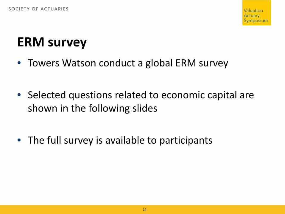
ERM survey• Towers Watson conduct a global ERM survey

• Selected questions related to economic capital are shown in the following slides

• The full survey is available to participants

14

The Rise of ERM as a Strategic PartnerEighth Biennial Global Enterprise Risk Management Survey

May 2015

© 2015 Towers Watson. All rights reserved. Proprietary and Confidential. For Towers Watson and Towers Watson client use only.

Economic capital in the ERM framework

© 2015 Towers Watson. All rights reserved. Proprietary and Confidential. For Towers Watson and Towers Watson client use only.towerswatson.com16

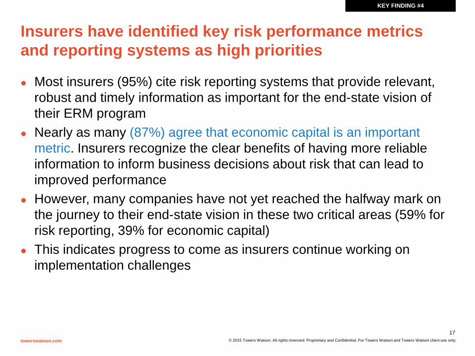
Insurers have identified key risk performance metrics and reporting systems as high priorities

Most insurers (95%) cite risk reporting systems that provide relevant, robust and timely information as important for the end-state vision of their ERM program

Nearly as many (87%) agree that economic capital is an important metric. Insurers recognize the clear benefits of having more reliable information to inform business decisions about risk that can lead to improved performance

However, many companies have not yet reached the halfway mark on the journey to their end-state vision in these two critical areas (59% for risk reporting, 39% for economic capital)

This indicates progress to come as insurers continue working on implementation challenges

towerswatson.com © 2015 Towers Watson. All rights reserved. Proprietary and Confidential. For Towers Watson and Towers Watson client use only.

17

KEY FINDING #4

Boards give positive feedback on the ability to leverage the results from EC models…

Some of the most common positive feedback mentioned include: Growing influence and integration of risk management framework into key

management decisions Clear and well supported identification of risks. Improved understanding

and awareness Comprehensive risk reporting and assessment capability Clear and well integrated risk appetite Improved risk awareness culture embedded in operations Leveraging results from economic capital models, allocating capital and

making risk-adjusted decisions Well established governance procedures Development and implementation of ORSA is well received by the board


18towerswatson.com

What feedback on positive impacts and development areas have you received from your board and/or senior executive team about the performance of your ERM framework and capabilities over the last 24 months?Q.2

ERM USE, PERFORMANCE AND PRIORITIES

Global resultsBase: Those giving a valid answer (n varies). Positive impact: n = 314, Development areas: n = 302.

…and expect further developments in the coming years

Some of the most common development areas mentioned include: Developing a risk culture within the organization Embedding ERM concepts (e.g. risk culture, risk appetite) in daily

operations and strategic decisions Developing and refining Economic Capital Models and link results to

management decision-making Allocating capital to risk types and lines of business to maximize risk-

adjusted return on capital Increasing/improving stress testing Achieving regulatory compliance and complete ORSA Improving data, IT infrastructure, dashboards, granularity, documentation


19towerswatson.com


What feedback on positive impacts and development areas have you received from your board and/or senior executive team about the performance of your ERM framework and capabilities over the last 24 months?Q.2

Global resultsBase: Those giving a valid answer (n varies). Positive impact: n = 314, Development areas: n = 302.

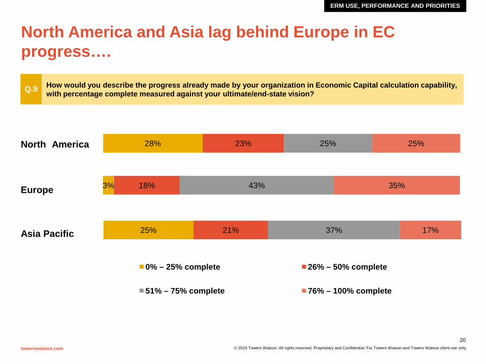
North America and Asia lag behind Europe in EC progress….



How would you describe the progress already made by your organization in Economic Capital calculation capability, with percentage complete measured against your ultimate/end-state vision?Q.9

20

28% 23% 25% 25%

3% 18% 43% 35%Europe

25% 21% 37% 17%

0% – 25% complete 26% – 50% complete

51% – 75% complete 76% – 100% complete

Asia Pacific

North America

…but is a high priority for improvement in North America over the next 2 years



How does Economic Capital calculation capability rank in your improvement priorities for the next 24 months? Please rank up to three, with the first item selected being the highest priority and the third being the least important.Q.11

21

3%

12%

17%

6%

9%

15%

10%

3%

9%

Asia Pacific

Europe

North America

Rank 1 Rank 2 Rank 3

What measures are used to set risk appetite?

• Regulatory capital threshold• 87% of European insurers use a regulatory capital threshold, compared to

81% in North America and 83% in Asia Pacific.

• Economic capital threshold• 72% of European insurers use an economic capital threshold compared to

only 47% in North America and 50% in Asia Pacific.

• Rating agency capital threshold• 35% of European insurers use a rating agency capital threshold compared

to 66% in North America and 17% in Asia Pacific.

• Most companies use look at regulatory capital for risk appetite threshold setting. In addition, Europe and APAC are looking at economic capital whereas North America is looking at rating agency capital

RISK APPETITE


22

Improving risk and economic capital models and risk management culture are the top two primary areas of focus for insurers relating to S&P ratings criteria

UNITED STATES — REGULATION AND RATINGS AGENCIES

Base: United States insurers rated by S&P and giving a valid answer (percentages exclude non-respondents and ‘None of these –no improvements planned’).

Which areas relating to S&P’s ERM rating criteria are your primary focuses for improvement? Please select up to two.US.8


43%

32%

15%

53%

32%

Risk management culture (includinggovernance and appetite)

Risk controls

Emerging risk management

Risk and economic capital models

Strategic risk management

United States

Risk Identification and Assessment


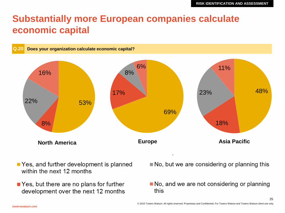
Substantially more European companies calculate economic capital

RISK IDENTIFICATION AND ASSESSMENT

Does your organization calculate economic capital?Q.20

towerswatson.com© 2015 Towers Watson. All rights reserved. Proprietary and Confidential. For Towers Watson and Towers Watson client use only.

25

53%

8%

22%

16%

69%

17%

8%6%

48%

18%

23%

11%

North America Europe Asia Pacific

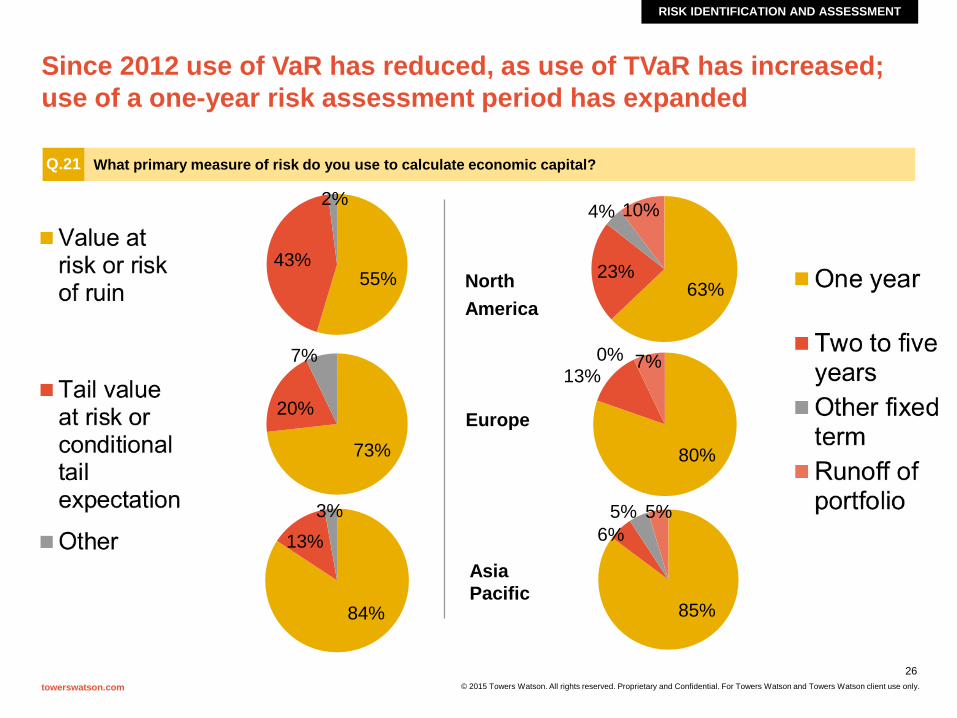
Since 2012 use of VaR has reduced, as use of TVaR has increased; use of a one-year risk assessment period has expanded


What primary measure of risk do you use to calculate economic capital?Q.21


26towerswatson.com

55%43%

2%

63%23%

4% 10%

NorthAmerica

73%

20%

7%

80%

13%0% 7%

Europe

84%

13%3%

85%

6%5%5%

Asia Pacific

NA P&C leads stochastic modelling, market and credit risk lags Europe



27

51%

46%

26%

35%

20%

7%

12%

25%

21%

47%

29%

12%

48%

26%

17%

27%

21%

25%

54%

23%

24%

7%

6%

7%

10%

14%

21%

38%

Market riskCredit risk

Life insurance riskP&C insurance risk

Operational riskLiquidity risk

Group risk

Stochastic approach Stress testing Factor-based Other

towerswatson.com

76%

63%

38%

62%

24%

32%

41%

14%

18%

41%

22%

37%

35%

28%

10%

20%

18%

16%

37%

26%

10%

0%

0%

3%

0%

2%

6%

21%




Group risk67%

58%

37%

77%

26%

33%

48%

23%

23%

37%

17%

19%

48%

20%

7%

14%

22%

3%

38%

7%

10%

4%

5%

5%

3%

17%

12%

23%




Group riskWhat methodology do you use for your economic capital calculations for each of the following risks? Please select one in each row.Q.22

North America

Europe

Asia Pacific

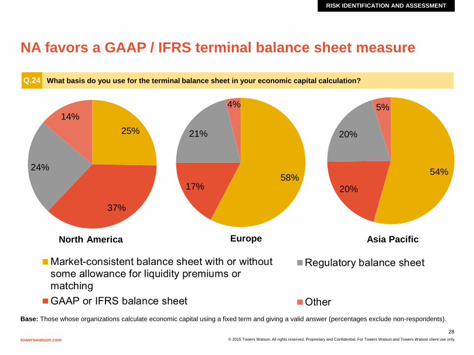
NA favors a GAAP / IFRS terminal balance sheet measure

Base: Those whose organizations calculate economic capital using a fixed term and giving a valid answer (percentages exclude non-respondents).


What basis do you use for the terminal balance sheet in your economic capital calculation?Q.24


28towerswatson.com

25%

37%

24%

14%

58%17%

21%

4%

54%

20%

20%

5%

North America Europe Asia Pacific

Most market consistent terminal balance sheets do not include any adjustment to the risk-free rate


What adjustment do you apply when deriving the risk-free rate in your terminal balance sheet?Q.25


29towerswatson.com

75%

8%

4%

6%

0%

8%

40%

10%

7%

23%

10%

10%

45%

15%

5%

10%

25%

0%

No fundamental adjustment — risk-free rate is based on swaps or government bonds (possibly with minor adjustment

for credit risk of swap/government bond issuer)

A different allowance for credit spread with adjustment forexpected defaults, default risk premium and projected forced

sales of assets

Solvency II matching adjustment (with or withoutmodification)

Solvency II volatility adjustment (with or withoutmodification)

Liquidity premium based on the Solvency II QuantitativeImpact Study (QIS 5) approach (with or without modification)

OtherNorth America

Europe

Asia Pacific

Most run-off approaches do not have explicit checks for interim solvency or cash-flow deficiencies


Which of the following most closely resembles your approach to checking interim solvency or cash-flow deficiencies in your economic capital calculation?Q.26


30towerswatson.com

30%

20%

0%

50%

The capital metric is based on the greatest presentvalue of accumulated deficiencies

The capital calculation includes explicit checks forinterim solvency using a projected balance sheet at

intermediate time periods prior to the end of theprojection

The capital calculation includes explicit checks forcash-flow deficiencies (net of reinvestment or

borrowing strategies) at intermediate time periodsprior to the end of the projection

There are no explicit checks for interim solvency orinterim cash-flow deficiencies

North America

Aggregation of risks is most commonly performed using a variance-covariance formula


What methodology do you use for aggregating risk across your overall business?Q.27


31towerswatson.com

Simple addition of risk capital results for each risk orbusiness unit

Variance-covariance formula (using correlation matrix)applied to risk capital results for each risk or business unit

Simulation-based approach using a large number of multi-risksimulations, within which the dependency structure among

risks is captured

Mixture of variance-covariance formula and simulationapproach (e.g., simulation approach within major risk

buckets, with overall aggregation by formula)

Other

14%

26%

38%

18%

4%

6%

45%

32%

13%

4%

10%

56%

10%

18%

5% North America

Europe

Asia Pacific

1 Year Var Calculation

32

1 year VaR models• In addition to valuation complexities, there are other

difficulties in calculating a 1 year VaR capital• In particular you need a method to overcome the

nested stochastic problem • A number of methods are available to do this• Two popular methods are discussed below:

– The covariance matrix – Simulation and proxy

33

34

Covariance Matrix• The simplest method to calculate capital is via a covariance

matrix:

• Determine the 99.5% instantaneous shock for each individual risk

• Calculate change in balance sheet for each risk

• Assume that risks follow a multivariate normal (elliptical) distribution

• Aggregate capital requirement = “root sum squares”

35

Covariance Matrix• Problem with this approach

• To calculate distribution of capital we need to know:– Joint probabilities of economic (and other) events occurring– What the balance sheet will look like under these events

• Covariance matrix assumes:– Risk factors have a joint normal distribution– Individual risks are linear

• Both are important for a capital calculation

36

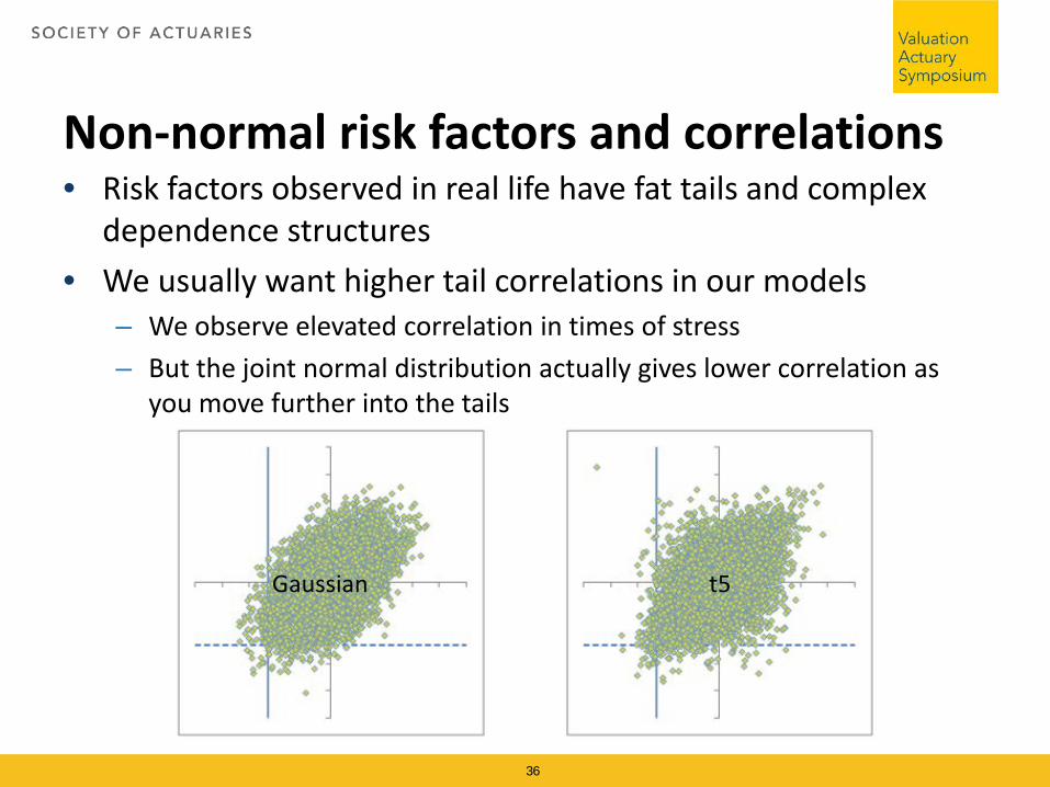
Non-normal risk factors and correlations• Risk factors observed in real life have fat tails and complex

dependence structures• We usually want higher tail correlations in our models

– We observe elevated correlation in times of stress– But the joint normal distribution actually gives lower correlation as

you move further into the tails

Gaussian t5

37

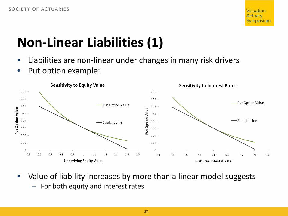
Non-Linear Liabilities (1) • Liabilities are non-linear under changes in many risk drivers• Put option example:

• Value of liability increases by more than a linear model suggests– For both equity and interest rates

38

Non-Linear Liabilities (2)• Liabilities also have joint non-linearity• Put option joint behaviour:

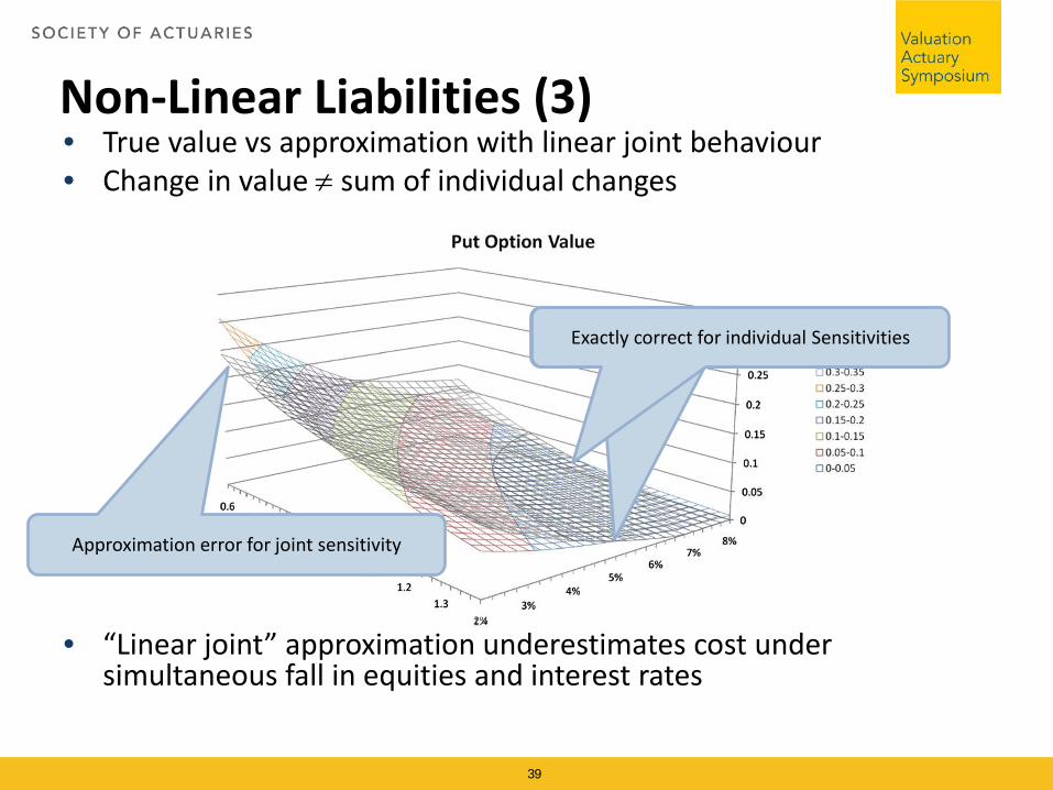
• True value vs approximation with linear joint behaviour• Change in value ≠ sum of individual changes

• “Linear joint” approximation underestimates cost under simultaneous fall in equities and interest rates

39

Non-Linear Liabilities (3)

Exactly correct for individual SensitivitiesExactly correct for individual Sensitivities

Approximation error for joint sensitivity

• Value is individually and jointly linear• Only correct in some places (a bit like a stopped clock)

• Tend to underestimate capital when liabilities are non-linear

40

Covariance Matrix Implicit Assumption

• Error is potentially larger than original liability

• Correct for a ring in the centre– This area does not correspond to area where joint behaviour is important– Important area is determined by correlation

41

Error of Linear Approximation

Covariance matrix summary• There are substantial flaws in the covariance matrix

methodology• These tend to under-estimate capital for life business• Even though it is the basis of the SII standard

formula, most large insurance companies and those with material options and guarantees have been forced to adopt an internal model and have been strongly discouraged from basing it on the covariance matrix approach– *Except for in France

42

Stochastic approach• A better way to calculate capital is to use the

stochastic approach• Simulate a joint distribution of your risk factors over

1 year– Using fat tails, advanced copulea etc

• And then calculate the balance sheet in each one of these scenarios

• And take a VaR / CTE measure from these outcomes

43

With the one-year approach, Required EC is based on the potential change in value over a one-year risk horizon

44

T = 0 T = 1

0.5% probability

0.05% probability

Available Economic Capital (AEC)

Expected

Probability of outcom

e

Scen1

Scen 100,000

Market Value Assets

BEL1

AEC

RM

Market Value Assets

BEL1

AEC

RM

Market Value Assets

BEL1

AEC

RM

Risk factor

Loss

Universal Life

The most advanced insurers are using stochastic, all-risk aggregation by simulation and proxy models

Random Number

Generator

Dependency

Risk factor

Probability

Interest rate

Risk factorLoss

Risk factor

Loss

Risk factor

Probability

Mortality

Σ= MortalityΣ= Interest Rate

Σ= Loss ULΣ= Loss Annuities

Σ= Total

Parametric distributions

Cat model output

Stress test fittingStochastic model output

FungibilityTaxReinsurance

Loss amount

Probability

Required capital

Risk factor

Loss

Payout Annuities

45

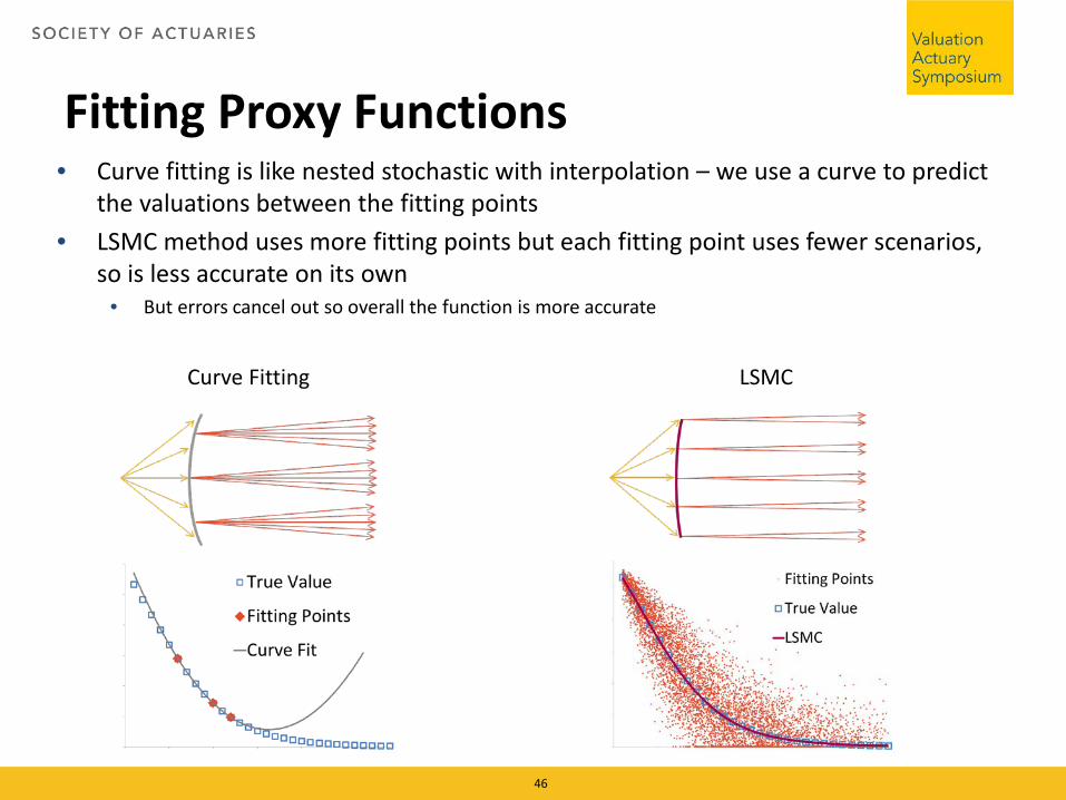
Fitting Proxy Functions• Curve fitting is like nested stochastic with interpolation – we use a curve to predict

the valuations between the fitting points• LSMC method uses more fitting points but each fitting point uses fewer scenarios,

so is less accurate on its own• But errors cancel out so overall the function is more accurate

46

Curve Fitting LSMC

Proxy Function Fitting Process (LSMC)

47

T0 T1 End

Risk Neutral

Real World

T0 End

Risk Neutral

Real World

1. Choose timestep 2. Choose risk drivers 3. Create fitting scenarios

4. Run through ALM model 5. Preform regression 6. Validate function

Benefits of the simulation and proxy based approach• Runtime is significantly reduced compared to the brute force

nested stochastic method• Significant limitations in the covariance matrix-based formula are

overcome. – Joint-normal risk distribution assumption– Linear loss function assumption

• Proxy functions can be accurately fitted and give a very good representation of the liabilities in multiple risk dimensions– This allows you to get better risk metrics for each risk as well as losses

experienced when risk factors change together• Risk factor scenarios can include complex, non-normal distributions

and copulae– This gives extra realism in the risk dynamics and more accurate risk

assessment

48

Uncertainties and limitations• Even in the best EC models, a number of

uncertainties and limitations remain– Valuation basis– Estimating risk tails– Estimating correlations / dependencies (especially in the

tails)– Treatment of operational risk– Treatment of risk calibration

49

Point in time vs Through the cycle (I)• Conditional vs un-contitional calibration• We take it for granted that market data like the yield

curve should be updated at each calibration period• But also the risk can be conditional

– Recent history vs long term history– Really some risks are naturally conditional / semi conditional

• Interest rate risk is proportional to level of rates– Option implied volatilities as a good predictor of future short

term market risk• Should we look to option markets to calibrate our risk distributions?• We would end up with super-pro-cyclical regime• But the cost of hedging / value of hedges would be well aligned with

changes in capital requirements

50

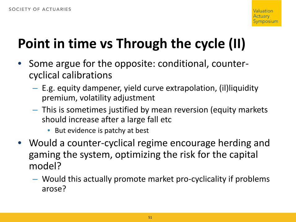
Point in time vs Through the cycle (II)• Some argue for the opposite: conditional, counter-

cyclical calibrations– E.g. equity dampener, yield curve extrapolation, (il)liquidity

premium, volatility adjustment– This is sometimes justified by mean reversion (equity markets

should increase after a large fall etc• But evidence is patchy at best

• Would a counter-cyclical regime encourage herding and gaming the system, optimizing the risk for the capital model?– Would this actually promote market pro-cyclicality if problems

arose?

51

Case StudyValuation Actuary Symposium 2015

8/31/2015Prabhdeep Singh, FSA, CERA, MAAA

Disclaimer: For educational purposes only. This is not a professional advice and does not represent an actuarial opinion or

communication. Views and opinions expressed are of the individuals only and not of the Guardian nor of the Society of Actuaries.

Agenda About the Guardian and the Individual Life business Economic Capital (EC) definition Practical considerations in

Setting up the EC organization Setting up EC models and scenarios Aggregating and analyzing the results

The Guardian The Guardian is a multi-line mutual life insurer domiciled in New York. The company

was founded in 1860.

It is owned by its policyholders and managed to their benefit.

It is a Fortune 500 company with over $6.8 billion in capital and $1.3 billion in operating income and one of the largest mutual insurers.

It has approximately 6,000 employees and more than 3,000 financial representatives in the United States.

Its businesses include Life Insurance, Employee Benefits, Annuities, Disability Income Insurance, Investments and 401(k).

Life Insurance

Employee Benefits

AnnuitiesDisability Income

Insurance

Investments and 401(k)

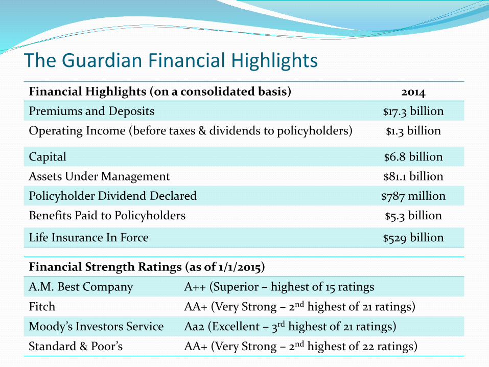
The Guardian Financial HighlightsFinancial Highlights (on a consolidated basis) 2014Premiums and Deposits $17.3 billion

Operating Income (before taxes & dividends to policyholders) $1.3 billion

Capital $6.8 billion

Assets Under Management $81.1 billion

Policyholder Dividend Declared $787 million

Benefits Paid to Policyholders $5.3 billion

Life Insurance In Force $529 billion

Financial Strength Ratings (as of 1/1/2015)

A.M. Best Company A++ (Superior – highest of 15 ratings

Fitch AA+ (Very Strong – 2nd highest of 21 ratings)

Moody’s Investors Service Aa2 (Excellent – 3rd highest of 21 ratings)

Standard & Poor’s AA+ (Very Strong – 2nd highest of 22 ratings)

The Guardian Legal Organization

The Guardian Life Insurance Company of America (Life Insurance and Employee Benefits)

The Guardian Insurance and Annuity Company,

Inc.(Annuities and 401(k))

Berkshire Life Insurance Company of America

(Disability Income Insurance)

Guardian Investor Services LLC, Park Avenue

Institutional Advisors LLC, RS Investment

Management Co. LLC, and others (Investments)

The Guardian Life Insurance Company of America (GLICOA) has several subsidiaries and affiliates. Not all of them are listed here. The primary business of the legal entity is described in the parentheses.

The Guardian Insurance and Annuity Company (GIAC) and Berkshire Life Insurance Company of America (BLICOA) are wholly owned subsidiaries of GLICOA.

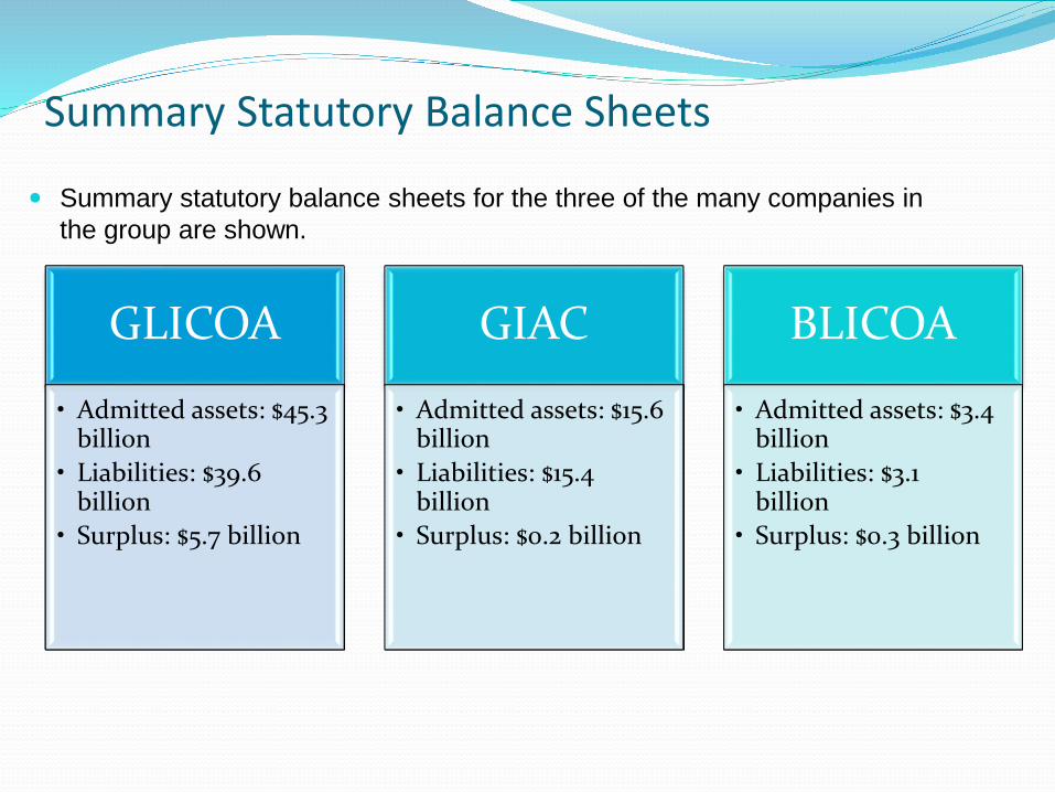
Summary Statutory Balance Sheets

GLICOA

• Admitted assets: $45.3 billion

• Liabilities: $39.6 billion

• Surplus: $5.7 billion

GIAC




BLICOA




Summary statutory balance sheets for the three of the many companies in the group are shown.

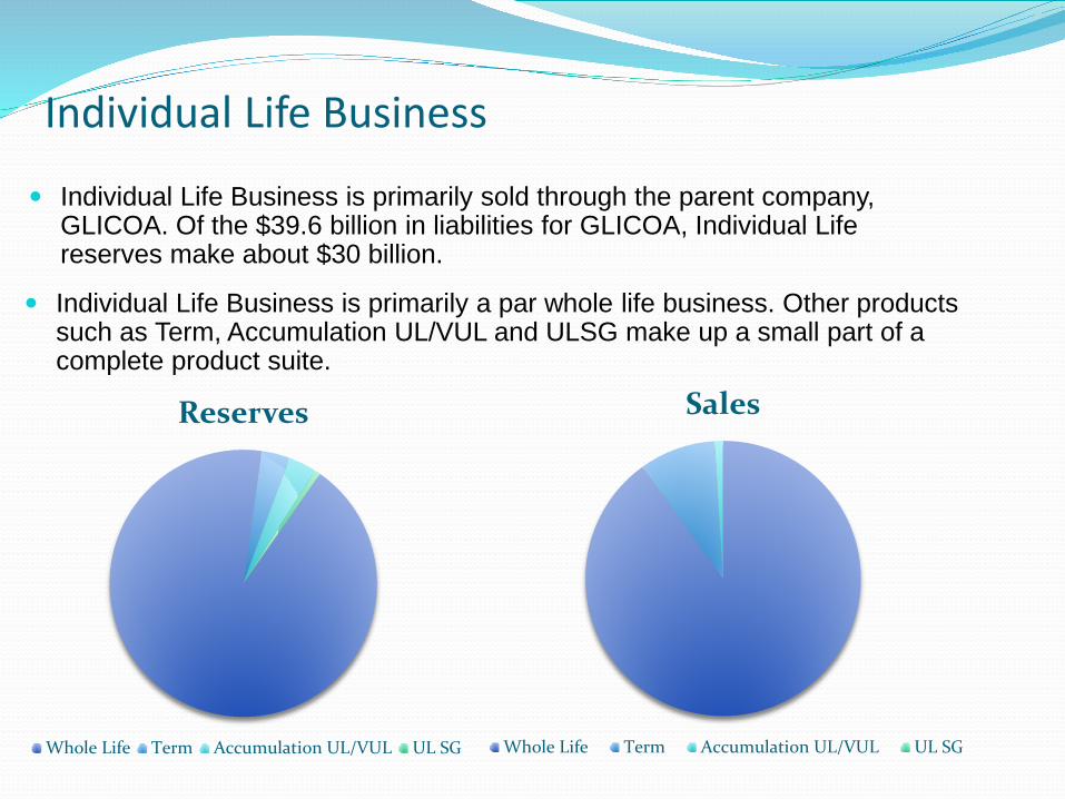
Individual Life Business

Individual Life Business is primarily sold through the parent company, GLICOA. Of the $39.6 billion in liabilities for GLICOA, Individual Life reserves make about $30 billion.

Reserves

Whole Life Term Accumulation UL/VUL UL SG

Sales

Whole Life Term Accumulation UL/VUL UL SG

Individual Life Business is primarily a par whole life business. Other products such as Term, Accumulation UL/VUL and ULSG make up a small part of a complete product suite.

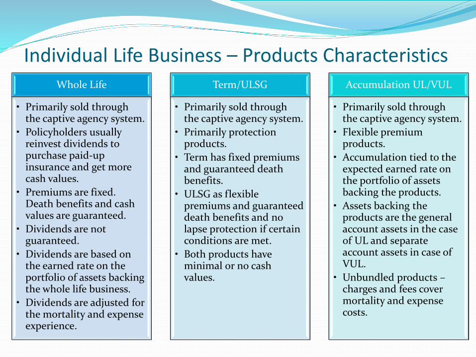
Individual Life Business – Products CharacteristicsWhole Life

• Primarily sold through the captive agency system.

• Policyholders usually reinvest dividends to purchase paid-up insurance and get more cash values.

• Premiums are fixed. Death benefits and cash values are guaranteed.

• Dividends are not guaranteed.

• Dividends are based on the earned rate on the portfolio of assets backing the whole life business.

• Dividends are adjusted for the mortality and expense experience.

Term/ULSG


• Primarily protection products.

• Term has fixed premiums and guaranteed death benefits.

• ULSG as flexible premiums and guaranteed death benefits and no lapse protection if certain conditions are met.

• Both products have minimal or no cash values.

Accumulation UL/VUL


• Flexible premium products.

• Accumulation tied to the expected earned rate on the portfolio of assets backing the products.

• Assets backing the products are the general account assets in the case of UL and separate account assets in case of VUL.

• Unbundled products –charges and fees cover mortality and expense costs.

Individual Life Business – Product RisksWhole Life

• Interest Rate Risk• Risk of interest rates

staying persistently low

• Risk of interest rates rising sharply.

• Asset default (credit) risk

• Inflation risk• Mortality risk,

including pandemic risk

• Lapse risk, other than disintermediation risk

• Operational risks

Term/ULSG

• Interest rate risk – risk of interest rates staying persistently low.


• Inflation risk• Mortality risk, mostly

mitigated by reinsurance treaties.

• Lapse risk – primarily pricing risk

• Operational risks.

Accumulation UL/VUL

• Interest rate risk for Accumulation UL products• Risk of interest rates

staying persistently low

• Risk of interest rates rising sharply.


• Mortality risk, including pandemic risk

• Equity risk for VUL, low fee generation

• Operational risks

Economic Capital Definition Sufficient surplus to fulfill our obligations to policyholders

over a 30 year period with high degree of confidence

OR

Sufficient surplus to assure statutory assets are greater than statutory liabilities over a 30 year period with high degree of confidence.

This definitions lends itself to a liability runoff approach, instead of a one-year mark-to-market approach.

Economic Capital - Mechanics Generate 2000 scenarios for each risk for 30 years Develop an integrated set of scenarios to represent 2000

possible futures Start with Assets equal to Reserves (i.e. Surplus = 0) Project Assets and Reserves for those 2000 integrated

scenarios For each scenario determine the greatest present value of

accumulated deficiency (GPVAD). Rank scenarios based on GPVAD. Average the worst 20 scenarios to obtain Economic Capital.

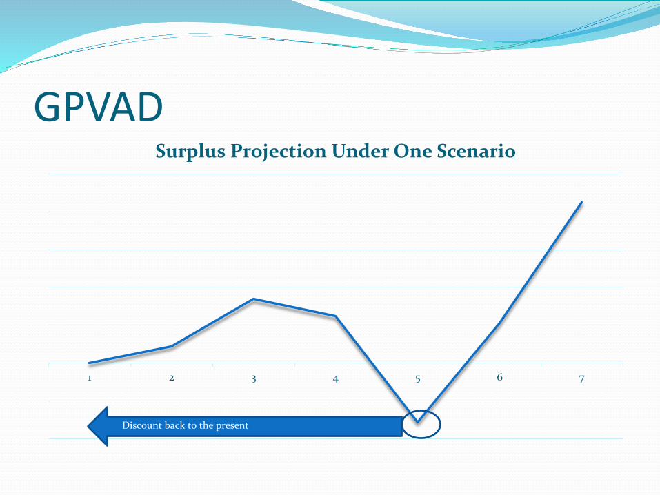
GPVAD

1 2 3 4 5 6 7

Surplus Projection Under One Scenario

Discount back to the present

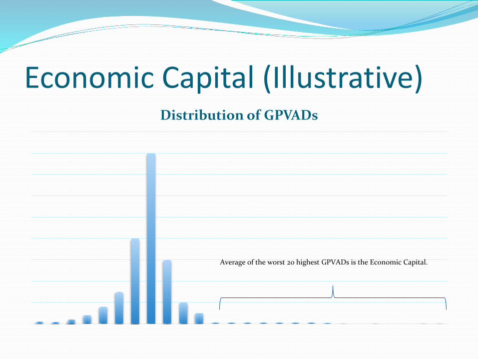
Economic Capital (Illustrative)Distribution of GPVADs

Average of the worst 20 highest GPVADs is the Economic Capital.

Practical Considerations

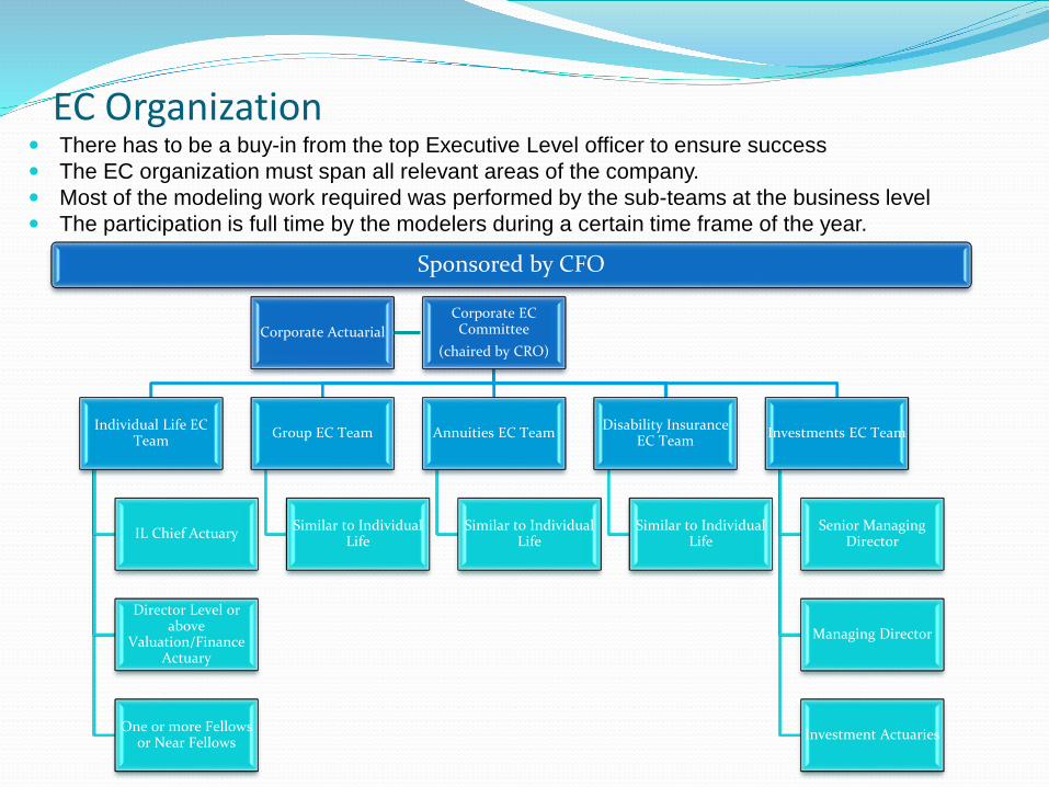
EC Organization

Corporate ActuarialCorporate EC Committee

(chaired by CRO)

Individual Life EC Team

IL Chief Actuary

Director Level or above

Valuation/Finance Actuary

One or more Fellows or Near Fellows

Group EC Team

Similar to Individual Life

Annuities EC Team


Disability Insurance EC Team


Investments EC Team

Senior Managing Director

Managing Director

Investment Actuaries

There has to be a buy-in from the top Executive Level officer to ensure success The EC organization must span all relevant areas of the company. Most of the modeling work required was performed by the sub-teams at the business level The participation is full time by the modelers during a certain time frame of the year.

Sponsored by CFO

EC Organization Getting to here from there has been a journey. Initially engage outside consultant who did virtually all the work for us. Then, developed EC results in-house and gave ourselves time to improve the process and

models. Finally, had outside consultants review our process, models, and results. Still improving processes and models.

2007: Engage Outside Consultant•Virtually all work is done by the consultant

2008: Engage Outside Consultant•Virtually all work is done by the consultant •Enhance the analysis

2009-2010: No EC results produced.

2011: Use lessons learned from 2007-2008 engagement to develop EC results in-house.•Leverage CFT models•ORSA, Rating Agency, and Industry trends allow buy-in from Executive leadership.

2012-2014: Continuously improve models and processes.• Engage outside consultant

to review process, models and results.

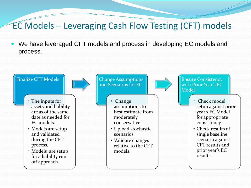
EC Models – Leveraging Cash Flow Testing (CFT) models

We have leveraged CFT models and process in developing EC models and process.

Finalize CFT Models

• The inputs for assets and liability are as of the same date as needed for EC models. • Models are setup

and validated during the CFT process.• Models are setup

for a liability run off approach

Change Assumptions and Scenarios for EC

• Change assumptions to best estimate from moderately conservative. • Upload stochastic

scenarios.• Validate changes

relative to the CFT models.

Ensure Consistency with Prior Year’s EC Model

• Check model setup against prior year’s EC Model for appropriate consistency. • Check results of

single baseline scenario against CFT results and prior year’s EC results.

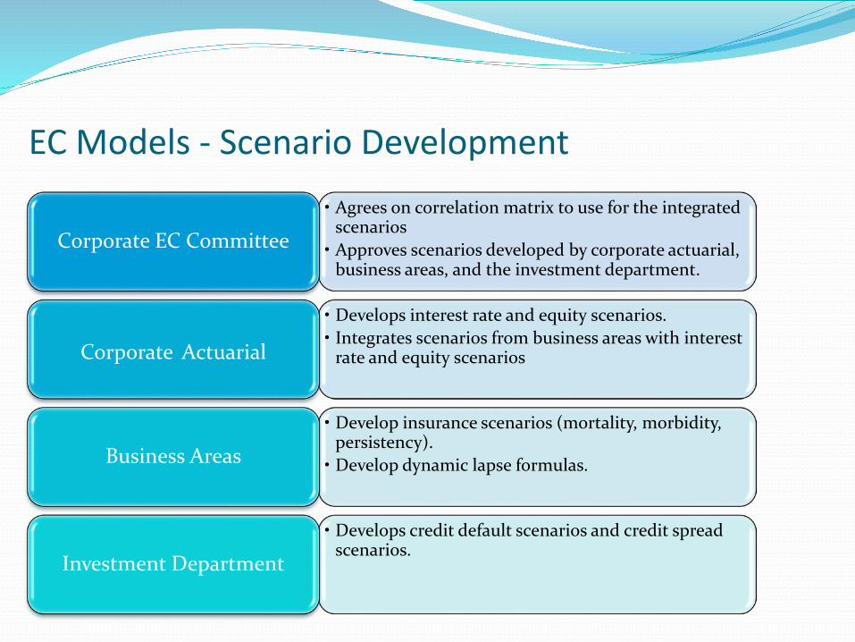
EC Models - Scenario Development• Agrees on correlation matrix to use for the integrated

scenarios• Approves scenarios developed by corporate actuarial,

business areas, and the investment department.Corporate EC Committee

• Develops interest rate and equity scenarios.• Integrates scenarios from business areas with interest

rate and equity scenariosCorporate Actuarial

• Develop insurance scenarios (mortality, morbidity, persistency).• Develop dynamic lapse formulas.Business Areas

• Develops credit default scenarios and credit spread scenarios.

Investment Department

EC Models - Scenario Generators Economic Scenario Generators

For interest rate scenarios we had several choices: Use the American Academy of Actuaries scenario generator Use the Casualty Actuarial Society scenario generator Use the scenario generator that came with the modeling software. Buy a high-end economic scenario generator from a vendor. Develop an in-house scenarios generator.

We had similar choices for the equity scenarios. We decided to go with the scenario generator that came with the modeling software.

This was the scenario generator that we had been using regularly with VACARVM. It was the one we were most familiar with and required least amount of investment.

For the credit risk scenarios, we had in-house expertise in developing the model and the scenarios. Therefore, we leveraged that.

For inflation our options were an expensive economic scenario generator from a vendor or an in-house simple model. We went with the latter.

Dynamic lapse formula for the life insurance business was developed and calibrated in-house.

Mortality scenario generator was developed in-house. Lapse scenario generator was developed in-house. Operational risk scenarios were developed in-house by adopting a tool provided

by a vendor.

EC Models - Interest Rate Scenario Generator Use a log-normal Hull-White model, aka Black-Krasinski model for the short rate (1-year

treasury rate), call this the yield curve level. Use a normal HW model for the difference between the short rate and the long rate (30-

year), call this the yield curve slope. Use the normal HW model for the difference between the medium rate (7-year rate) and

the medium rate implied by the level and the slope, call this the yield curve curvature. Use cubic splines and other interpolation/extrapolation methods to determine other

points on the yield curve. The following graphs illustrate these key features of yield curve changes.

0

1

2

3

4

5

1-Year 10-Year 20-Year 30-Year

Change in Level

Original Parallel Shift - Down

Parallel Shift - Up

0

1

2

3

4

5


Change in Slope

Original Flattening Steepening

0

1

2

3

4

5


Change in Curvature

Original Negative Positive

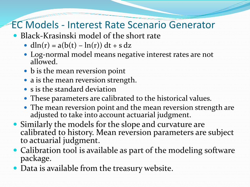
EC Models - Interest Rate Scenario Generator Black-Krasinski model of the short rate

dln(r) = a(b(t) – ln(r)) dt + s dz Log-normal model means negative interest rates are not

allowed. b is the mean reversion point a is the mean reversion strength. s is the standard deviation These parameters are calibrated to the historical values. The mean reversion point and the mean reversion strength are

adjusted to take into account actuarial judgment. Similarly the models for the slope and curvature are

calibrated to history. Mean reversion parameters are subject to actuarial judgment.

Calibration tool is available as part of the modeling software package.

Data is available from the treasury website.

EC Models - Interest Scenario Generator

Percentile Year 0 10 15 20 30Min 0.1% 0.9% 1.0% 0.9% 1.1%1% 0.1% 1.3% 1.4% 1.3% 1.4%5% 0.1% 1.7% 1.8% 1.8% 1.8%

10% 0.1% 2.0% 2.1% 2.0% 2.0%25% 0.1% 2.5% 2.6% 2.6% 2.6%50% 0.1% 3.4% 3.5% 3.5% 3.4%75% 0.1% 4.6% 4.8% 4.8% 4.8%90% 0.1% 6.1% 6.5% 6.5% 6.5%95% 0.1% 7.4% 8.1% 8.2% 7.9%99% 0.1% 10.4% 12.0% 13.1% 11.6%Max 0.1% 21.8% 23.4% 21.2% 23.4%

The following shows the stats for the short rate. We analyze the interest rate scenarios for several other statistics,

including yearly distributions for the medium and the long rate, overall distribution of interest rates, probabilities of breaching certain threshold how interest rates behave over time. For example, longest period

that interest rates stay persistently low? How fast interest rates rise?

Mortality Scenarios Five sources of mortality risk

Random fluctuations around expected Uncertainty in the estimate of the expected and the

random fluctuations Mortality volatility Uncertain mortality improvements Catastrophic mortality (pandemics)

State of research Most scientific research focused on population mortality No textbook model available to develop Mortality

Scenario Generator

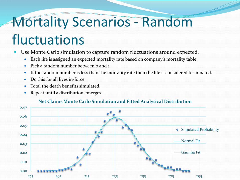
Mortality Scenarios - Random fluctuations Use Monte Carlo simulation to capture random fluctuations around expected.

Each life is assigned an expected mortality rate based on company’s mortality table. Pick a random number between 0 and 1. If the random number is less than the mortality rate then the life is considered terminated. Do this for all lives in-force Total the death benefits simulated. Repeat until a distribution emerges.

0.00

0.01

0.02

0.03

0.04

0.05

0.06

0.07

175 195 215 235 255 275 295

Net Claims Monte Carlo Simulation and Fitted Analytical Distribution

Simulated Probability

Normal Fit

Gamma Fit

Mortality Scenarios – Uncertain Estimates of Mean and Variance The mortality table is based on limited data Therefore, the true mortality rates are not known Past A/E ratios can indicate the amount uncertainty in the mortality

table. Use past A/E ratio to develop an empirical distribution to sample from.

The empirical distribution indicates what the mortality table could have been.

Adjust the mortality table based on the sample from the empirical distribution.

Mortality Scenarios – Volatility and Uncertain Trend Mortality is volatile (i.e. it would fluctuate even if

infinite sample size) There is a clear downward trend in mortality, however,

this trend is not certain. Furthermore, there are calendar year and cohort

effects. These are not taken into account when developing our mortality scenarios.

Mortality Scenarios Develop scenarios as follows:

Adjusted the distribution obtained from static Monte Carlo simulation for uncertainty in the mortality table by sampling an A/E ratio

from the empirical distribution. mortality volatility uncertain trend. Age and size of the business

Sample from the adjusted distribution the aggregate mortality rate

Mortality Scenarios- Pandemics Pandemic scenarios were modeled separately from the other

mortality risks. Frequency and Severity model, calibrated to 300 years of history

of pandemics, Adjust for the mitigations techniques available today (e.g.

vaccines, anti-virals and anti-biotics) Adjust for the unique distribution of deaths by age. Use the Poisson distribution for the frequency Use the Weibull distribution for the severity Use the Poisson model to simulate the time to next Pandemic. Then, sample from the Weibull distribution to determine the

severity of the Pandemic. Do this for 30 years and 2000 scenarios.

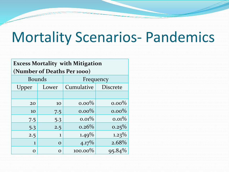
Mortality Scenarios- PandemicsExcess Mortality with Mitigation (Number of Deaths Per 1000)

Bounds FrequencyUpper Lower Cumulative Discrete

20 10 0.00% 0.00%10 7.5 0.00% 0.00%

7.5 5.3 0.01% 0.01%5.3 2.5 0.26% 0.25%2.5 1 1.49% 1.23%

1 0 4.17% 2.68%0 0 100.00% 95.84%

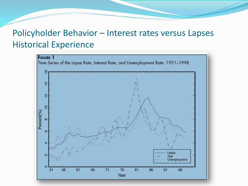
Policyholder Behavior – Interest rates versus Lapses Historical Experience

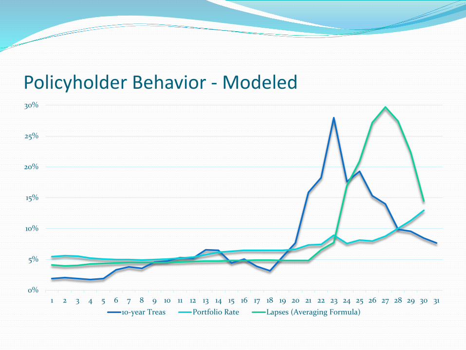
Policyholder Behavior - Modeled

0%

5%

10%

15%

20%

25%

30%

1 2 3 4 5 6 7 8 9 10 11 12 13 14 15 16 17 18 19 20 21 22 23 24 25 26 27 28 29 30 3110-year Treas Portfolio Rate Lapses (Averaging Formula)

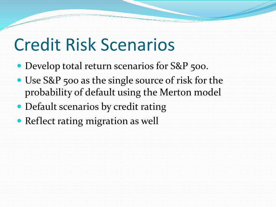
Credit Risk Scenarios Develop total return scenarios for S&P 500. Use S&P 500 as the single source of risk for the

probability of default using the Merton model Default scenarios by credit rating Reflect rating migration as well

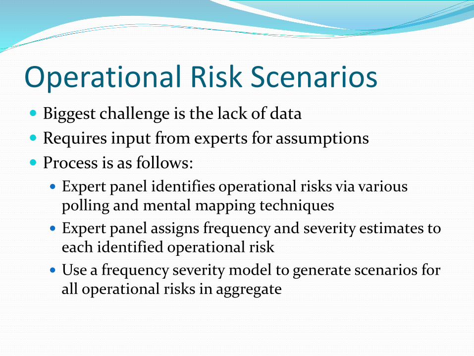
Operational Risk Scenarios Biggest challenge is the lack of data Requires input from experts for assumptions Process is as follows:

Expert panel identifies operational risks via various polling and mental mapping techniques

Expert panel assigns frequency and severity estimates to each identified operational risk

Use a frequency severity model to generate scenarios for all operational risks in aggregate

Inflation A simple regression was run between CPI-U and 20-

year treasuries Use the linear relationship to model inflation. Separate inflation scenarios were not generated

Model Efficiency Cluster modeling techniques can be used to reduce the

number of scenarios and the number of cells modeled to reduce the run time.

Distributed computing is also used to reduce the run time.

Individual Life Economic Capital

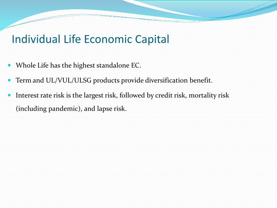
Whole Life has the highest standalone EC.

Term and UL/VUL/ULSG products provide diversification benefit.

Interest rate risk is the largest risk, followed by credit risk, mortality risk

(including pandemic), and lapse risk.

Aggregation Scenarios for all the risks (except operational) are pushed

through a t-copula model to generate integrated scenario set. Scenario set for each risk on a stand alone basis can be

thought of as a marginal distribution for that risk. These marginal distributions need to be combined to form

the joint distribution. We generated 2000 scenarios for four risks. A direct

combination would have required us to run 2000^4 scenarios! Instead sample quadruplets assuming a t-copula joins the

four marginal distributions Integrated scenario set is used to project surpluses as

discussed earlier.

Aggregation by Business Area

Economic Capital

Business (+) Individual Life(+) Annuities(+) Individual Disability Income(+) Group Employee Benefits(=) Business EC (before diversification)(-) Diversification Benefits(=) Business EC (after diversification)(+) Operational Risk(=) Total Economic Capital

Economic Capital reviewed for each business area Provides good summary of risks by product type Diversification of product closely reviewed to ensure possible realization. The different timing of

occurrences of the GPAD among different business areas is a contributor to the diversification benefit and is a direct result of the long-term run-off methodology.

Run with and without 5 years new business

Aggregation by Risk Type

Economic Capital

Business (+) Equity(+) Interest(+) Credit(+) Mortality(+) Morbidity(+) Lapse(=) Total Individual Risk(-) Correlation / Diversification Impact(=) Business EC (Inforce Only)

Economic Capital reviewed for each risk type Helpful in understanding which individual risks grow throughout the projection Run without new business 2,000 scenarios for each risk type run separately with the other risk types run at their

baseline

Rollforward Completed for inforce only currently

Capture the impact for each business unit of the changes of the following: Inforce change Market assumption change (interest, equity, credit defaults) Insurance assumption change (mortality, morbidity,

persistency, expenses) Model Updates Asset Portfolio revisions Addition of new products

Resource intensive

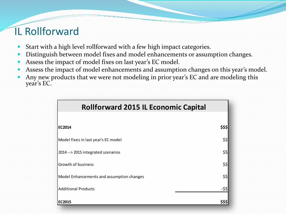
IL Rollforward Start with a high level rollforward with a few high impact categories. Distinguish between model fixes and model enhancements or assumption changes. Assess the impact of model fixes on last year’s EC model. Assess the impact of model enhancements and assumption changes on this year’s model. Any new products that we were not modeling in prior year’s EC and are modeling this

year’s EC.

EC2014 $$$

Model fixes in last year's EC model $$

2014 --> 2015 integrated scenarios $$

Growth of business $$

Model Enhancements and assumption changes $$

Additional Products -$$Other $ 1EC2015 $$$

Rollforward 2015 IL Economic Capital

IL Rollforward Provide more details behind each major category, if necessary.

Descriptive name of model fix 1 $$

Descriptive name of model fix 2 $$

Total $$

Model Fixes

2014 --> 2015 interest rate scenarios $$

2014 --> 2015 credit defaults $$

Total $$

Change in integrated scenarios

Descriptive name for Major Assumption Change 1 $$

Descriptive name for Major Assumption Change 2 -$$

Descriptive name for Model Enhancement 1 -$$

Total $$

Model Enhancements and Assumption Changes

Product 1 $$

Product 2 -$$

Product 3 -$$

Total -$$

Additional LOB

Additional Considerations Scenario count - ensure you have an acceptable level of

convergence in the tail Risk distributions – ensure that your distribution for each

significant risk is extreme enough to cover the tail. Correlations – test the impact of sensitivity to changes in

the correlation matrix Senior management may think that all correlations go to 1 in a crisis.

Documentation – ensure consistent documentation of the model meeting a model governance framework.

Actuarial Standards of Practice – ensure that standards are met.

Ensure model designed to support decision-making.

Questions?

session 17, introduction to economic capital 17, introduction to economic capital moderator: adam...

Documents